Parallel Algorithms for Masked Sparse Matrix-Matrix Products

Abstract.

Computing the product of two sparse matrices (SpGEMM) is a fundamental operation in various combinatorial and graph algorithms as well as various bioinformatics and data analytics applications for computing inner-product similarities. For an important class of algorithms, only a subset of the output entries are needed, and the resulting operation is known as Masked SpGEMM since a subset of the output entries is considered to be “masked out”.

Existing algorithms for Masked SpGEMM usually do not consider mask as part of multiplication and either first compute a regular SpGEMM followed by masking, or perform a sparse inner product only for output elements that are not masked out. In this work, we investigate various novel algorithms and data structures for this rather challenging and important computation, and provide guidelines on how to design a fast Masked-SpGEMM for shared-memory architectures. Our evaluations show that factors such as matrix and mask density, mask structure and cache behavior play a vital role in attaining high performance for Masked SpGEMM. We evaluate our algorithms on a large number of real-world and synthetic matrices using several real-world benchmarks and show that our algorithms in most cases significantly outperform the state of the art for Masked SpGEMM implementations.

1. Introduction

Masked sparse-sparse matrix multiplication (Masked SpGEMM) is the problem of computing the product of two sparse matrices only for the set of entries given by the nonzero structure of the mask. The mask can be thought as a sparse matrix whose pattern determines which elements should exist in the output matrix. While the first use of this primitive was in the context of triangle counting (azad2015parallel, ), its applications include any multi-source graph traversal where the mask serves as a filter to avoid rediscovery of previously discovered vertices. A canonical example is the multi-source betweenness centrality as implemented in GraphBLAS C API (bulucc2017design, ). Recently, Etter et al. (etter2021accelerating, ) showed how to accelerate tree-based inference methods using masked SpGEMM.

The existence of a mask in the multiplication introduces new optimization opportunities as well as challenges. A simple way to perform Masked SpGEMM is to compute the multiplication as if the mask does not exist and then apply the mask to the output matrix, which causes unnecessary computation if the overlap between the output matrix and the mask is low (see Figure 1). The mask needs to be considered as part of the multiplication to attain good performance, which is the focus of this work.

Most parallel SpGEMM methods rely on Gustavson’s algorithm (gustavson1978two, ), in which a row or a column of the output matrix is computed by accumulating the partial results produced by scaling rows or columns of one of the input matrices. The important design aspects of this algorithm, such as parallelization granularity, data structures (i.e., accumulators) used in the merging of partial results or whether to include a symbolic multiplication phase to determine the pattern of the output matrix, need to be reconsidered when a mask is part of the equation, even calling into question the viability of this algorithm for certain cases. Consider the computation of a row of the output matrix in which a considerable amount of flops is spent to get the result. If the mask does not require most of the entries in that row of the output matrix, one can avoid unnecessary computations by computing the unmasked entries with inner products instead of accumulating the scaled rows. Moreover, many graph algorithms rely on operations involving the complement of the mask, which is a way to express avoiding already visited nodes. This adds another design and optimization dimension to the Masked SpGEMM. Hence, not only the specific details of established SpGEMM algorithms must be reexamined for Masked SpGEMM, but also the viability of other less frequently-utilized algorithms and new issues arising because of masking.

Our code implementing our algorithms and data structures is available at https://github.com/PASSIONLab/MaskedSpGEMM.

Our contributions in this paper are:

• We describe push- and pull-based algorithms for Masked SpGEMM, and analyze/compare their memory behaviors.

• We design four different data structures to be used as accumulators in Masked SpGEMM: (i) Hash, (ii) Masked Sparse Accumulator, (iii) Masked Compressed Accumulator, and (iv) Heap. The Masked Compressed Accumulator is a novel accumulator we specifically designed for Masked SpGEMM, while the remaining three are enhancements to the accumulators utilized in plain SpGEMM.

• We discuss how to adapt these accumulators for Masked SpGEMM where the mask is complemented.

• In SpGEMM, a symbolic phase is often performed to compute the pattern of the output matrix prior to the numeric phase. We review the tradeoffs of including a symbolic phase when mask is part of the SpGEMM.

• We conduct extensive experiments on both synthetic and real-world matrices using graph processing applications to reveal the best design choices for a fast Masked SpGEMM.

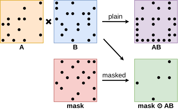
Figure 1. Plain vs. Masked SpGEMM. The masked output entries need not be computed. Also, mask may contain entries for which the multiplication does not produce an output.

2. Background and Notation

SpGEMM forms the computational backbone of many applications in linear algebra (Bell2012, ; Briggs2000, ; Griewank2003, ) and graph processing (Buluc2012, ; Gilbert2008, ; Penn2006, ; Dongen2008, ; azad2015parallel, ; Wolf2017, ; Selvitopi2020, ). This paper targets the performance of masked SpGEMM for graph processing as it is where the masked variant of SpGEMM is mainly utilized. Many graph algorithms can be expressed in terms of computations on sparse matrices due to the duality between graph and matrices. In this direction, GraphBLAS (bulucc2017design, ) is an effort to standardize the graph algorithm primitives in the language of linear algebra with an extended set of algebraic objects including semirings, upon which common sparse matrix computations such as SpMV or SpGEMM can be generalized.

We denote the Masked SpGEMM with $\mathbf{C}=\mathbf{M}\odot(\mathbf{A}\mathbf{B})$ on a semiring, where $\mathbf{M}\in\mathbb{S}^{m\times n}$ is the mask, $\mathbf{A}\in\mathbb{S}^{m\times k}$ and $\mathbf{B}\in\mathbb{S}^{k\times n}$ are the input sparse matrices, and $\mathbf{C}\in\mathbb{S}^{m\times n}$ is the output sparse matrix. Although the graph algorithms evaluated in this work utilize various semirings, we use the arithmetic semiring in our algorithms to keep the discussions simple. $\mathbf{A}_{ij}$ denotes a nonzero element of $\mathbf{A}$, and $\mathbf{A}_{i*}$ and $\mathbf{A}_{*j}$ respectively denotes $i$th row and $j$th column of $\mathbf{A}$. Note that we only utilize the pattern of the mask in Masked SpGEMM, hence the values in the mask are not evaluated and the type of the mask elements does not matter. We denote a vector with lowercase letters, i.e., $\mathbf{v}$, and an element of a vector is denoted with $\mathbf{v}_{i}$. We use the function $\mathit{nnz}(\cdot)$ to denote the number of nonzero elements in a matrix/vector, $\mathit{ncols}(\cdot)$ to denote the number of columns in a matrix/vector, and $\mathit{flops}(\cdot)$ to denote the number of floating point operations in a sparse matrix operation.

Algorithm 1 Row-parallel Gustavson SpGEMM (gustavson1978two, )

1:Sparse matrices $\mathbf{A}$, $\mathbf{B}$

2:Sparse matrix $\mathbf{C}$

3:$\mathbf{C}\leftarrow\emptyset$

4:for each row $\mathbf{A}_{i*}$ in matrix $\mathbf{A}$ in parallel  do

5:    for each nonzero $\mathbf{A}_{ik}$ in row $\mathbf{A}_{i*}$ do

6:        for each nonzero $\mathbf{B}_{kj}$ in row $\mathbf{B}_{k*}$ do

7:           $value\leftarrow\mathbf{A}_{ik}\cdot\mathbf{B}_{kj}$

8:           if $\mathbf{C}_{ij}\not\in\mathbf{C}_{i*}$ then

9:               insert $(\mathbf{C}_{ij}\leftarrow value)$ to $\mathbf{C}_{i*}$

10:           else

11:               $\mathbf{C}_{ij}\leftarrow\mathbf{C}_{ij}+value$                        

In our analyses, we assume that $\mathit{nnz}(\mathbf{A}),\mathit{nnz}(\mathbf{B}),\mathit{nnz}(\mathbf{M})\gg Z$, where $Z$ is the size of the last-level cache. For simplicity, we assume that a cache line can hold $L$ words, and that integers used in indexing and values used to store data are all the same size of a single word.

2.1. Storage Formats

Most popular formats for storing sparse matrices are Compressed Sparse Row (CSR), Compressed Sparse Column (CSC), Coordinate, and Doubly-Compressed Sparse Row/Column (DCSR/DCSC). In this work, we use the CSR format in most cases, with CSC only being used in a single case to improve performance of the inner product. We use CSR format for storing the mask. The CSR (CSC) format uses three arrays to store a sparse matrix: an array containing row (column) index pointers, an array containing column (row) indices of nonzeros, and an array containing values of nonzeros.

2.2. Design Issues and Challenges

There are four challenges to designing an efficient parallel SpGEMM running on multi-core systems: (i) irregular and random memory accesses when retrieving rows or columns of a sparse matrix, (ii) designing an accumulator to merge the partial results (if any), (iii) determining the pattern of the output matrix, and (iv) load imbalance. SpGEMM algorihms usually access the rows or columns of the sparse matrices randomly and this causes SpGEMM operation to be memory-bound rather than compute-bound, and often results in poor cache behavior. The addition of a mask to the SpGEMM only exacerbates these challenges.

A large portion of SpGEMM algorithms necessitate a data structure to accumulate the partial results to get the output matrix entries. For example in algorithms that rely on Gustavson’s algorithm (gustavson1978two, ), they may be used to accumulate the products in scaled rows/columns that correspond to the same output entry (Algorithm 1). Among common accumulators are sparse arrays (gilbert1992sparse, ; Patwary2015, ) (SPA), heaps (Azad2016, ; Liu2014, ), and hash tables (Deveci2017, ; Nagasaka2017, ). We investigate how to enhance these accumulators for Masked SpGEMM and propose a novel accumulator specifically designed for Masked SpGEMM.

Another issue is the unknown size and structure of the output matrix, which renders memory management difficult for the output matrix. Thus, SpGEMM algorithms sometimes perform two passes to complete the multiplication: the first pass to figure out the size and structure of the output matrix, referred to as the symbolic phase, and the second pass to compute its entries, referred to as the numeric phase. These are known as the two-phase algorithms, as opposed to the one-phase algorithms which allocate a large-enough memory at the beginning and perform the multiplication in a single numeric phase. Because the pattern of the mask partially determines the structure of the output matrix (note that the mask may contain unmasked entries for which there is no output entry), so one can possibly utilize the mask as a good starting point to approximate the size and the structure of the output. This can potentially render two-phase algorithms obsolete, a point we investigate in this work.

3. Related Work

SuiteSparse:GraphBLAS (SS:GB, which is the fastest compliant GraphBLAS implementation on multicore processors, initially used a dot-product algorithm for most masked SpGEMM calls (aznaveh2020parallel, ).Its most recent version (ssgrb21, ) also implements various hash-based and SPA-based codes that exploit mask. As a complete library, SS:GB supports multiple sparse matrix data structures, concepts such as “pending tuples” and “zombies” to take advantage of lazy evaluation in non-blocking mode of GraphBLAS, and graph specific optimization such as iso-valued matrices where all nonzero entries in the matrix have the same value. Therefore, it is not reasonable to perform an apples-to-apples comparison with our work, which focuses on algorithmic differences among various methods for performing masked SpGEMM. We are instead going to highlight the differences between our masked SpGEMM algorithms and those implemented in the latest version of SS:GB.

The GrB_mxm function of SuiteSparse:GraphBLAS, which covers the case of Masked SpGEMM, works with 4 different matrix formats: sparse, hypersparse, bitmap, and dense. The sparse case uses either the CSR or CSC formats. The hypersparse case uses either DCSR or DCSC (buluc2008representation, ). Our work is focused on the CSR format to isolate the algorithmic trade-offs involved in Masked SpGEMM. Our algorithms do not parallelize the formation of individual rows as we observed that there is plenty of coarse-grained parallelism across rows to avoid any load imbalance on the multi-core processors available today. The only other Masked SpGEMM implementation we are aware of is the GPU implementation from the GraphBLAST library (yang2019graphblast, ), which is based on dot products.

4. Classification of Algorithm Families

Our work on masking out certain entries of the output in sparse matrix computation has its primary motivations in the area of graph processing. In particular, the concept of masking has been first applied to sparse-matrix-vector multiplication to implement the direction-optimized graph traversal (yang2018implementing, ). The direction-optimization (beamer2012direction, ) is also known as push-pull (besta2017push, ) in the graph processing community. The standard way of processing a graph involves a frontier of active vertices that “pushes” information to their out-neighbors. The pull operation happens when the non-active (or previously unvisited, depending on the application) vertices “pulling” information from their in-neighbors.

This analogy with graph processing allows us to provide a classification of Masked SpGEMM algorithms into two main classes. The pull-based algorithms are those whose computation is mainly driven by the mask. For each potential entry $\mathbf{C}_{ij}$ in the output that is not masked out (i.e., $\mathbf{M}_{ij}\neq 0$), we “pull” information by inspecting the input sparse matrices to see if they can generate that output entry. The push-based algorithms are instead driven by the sparsity of the input matrices first, and they often utilize the mask as a filter before generating the output.

4.1. Pull-based Algorithms

Consider the naïve algorithm where for each $\mathbf{M}_{i,j}\neq 0$, we perform the sparse dot product $\mathbf{A}_{i*}\mathbf{B}_{*j}$. Since such sparse dot products are independent of each other, this algorithm has at least $O(\mathit{nnz}(\mathbf{M}))$-way parallelism, excluding any parallelism that can be extracted within the sparse dot product itself. This method is most efficiently implemented when $\mathbf{A}$ is stored in a row-major sparse storage such as CSR, and $\mathbf{B}$ is stored in a column-major sparse storage such as CSC (or vice versa), which is what we assume is the case in this study.

The described method, however, has one drawback: its poor temporal locality. Assume that we traverse the nonzeros of $\mathbf{M}$ in row-major order. Since rows of $\mathbf{A}$ are accessed consecutively, there is a significant reuse within rows. However, columns of $\mathbf{B}$ will be accessed in a scattered manner, with very little reuse. Given $\mathit{nnz}(\mathbf{B})\gg Z$ where $Z$ is the fast memory (cache) capacity, we can assume that each column access will fetch the whole column back from the main (slow) memory. For simplicity, we assume that each column of $\mathbf{B}$ is accessed the same number of times or each column of $\mathbf{B}$ has the same number of nonzeros $\mathit{nnz}(\mathbf{B})/n$. Either way, the amount of memory traffic of this method is: $\mathit{nnz}(\mathbf{A})+\mathit{nnz}(\mathbf{M})\Big{(}1+\frac{\mathit{nnz}(\mathbf{B})}{n}\Big{)}.$

4.2. Push-Based algorithms

There are many push-based SpGEMM algorithms. In this section, we focus on the most well-known row-by-row version due to Gustavson (gustavson1978two, ), also shown in Algorithm 1. In this algorithm, the $i$th row of the output is computed as a linear combination of $k$th rows of $\mathbf{B}$ where $\mathbf{A}_{ik}\neq 0$. This algorithm naturally parallelizes over rows as there are no dependencies. However, using a sparse accumulator (SPA) increases the cache load as one dense vector per row is used for accumulation. To overcome this, researchers have used data structures ranging from priority queues to hash tables to merge sparse rows of $\mathbf{B}$.

The formation of $\mathbf{C}_{i*}$ exhibits five memory access patterns:

1. Unit-stride read access to nonzeros within a row of $\mathbf{A}$.

2. Random-like read access to row pointers of $\mathbf{B}$.

3. Stanza-like read access to nonzeros of $\mathbf{B}$: small blocks (stanzas) of consecutive elements are fetched from effectively random locations in memory.

4. Random-like read and write access to the sparse accumulator (the scatter/accumulate step) for updating values.

5. Unit-stride write access for outputting $\mathbf{C}_{i*}$.

The choice of the data structure only changes the $4$th type of access where we can improve cache utilization with more compact data structures. The first three memory access patterns are canonical for row-by-row algorithms, i.e., they persist even if we replace the SPA with a priority queue or a hash table. As long as we use the push paradigm, those three memory accesses are also not affected by the use of a mask.

To analyze memory traffic costs, we make two reasonable assumptions: (1) the cache line length $L$ is smaller than the matrix dimension, i.e. $n>L$, and (2) the bandwidth of the first matrix is larger than the cache size, i.e. $\beta(\mathbf{A})>Z$. The matrix bandwidth $\beta(\mathbf{A})$ is the smallest non-negative integer $k$ such that $\mathbf{A}_{ij}\neq 0$ for $\lvert i-j\rvert>k$. Corollaries of Assumption 2 when performing $\mathbf{A}\mathbf{B}$ using a row-by-row algorithm are (a) row pointers of $\mathbf{B}$ are not cached, and (b) accesses to column ids and values of distinct rows of $\mathbf{B}$ are not cached.

The memory traffic incurred due to the first pattern is trivially $O(\mathit{nnz}(\mathbf{A}))$. The memory cost of the second pattern is $O(\mathit{nnz}(\mathbf{A})\cdot L)$ due to assumption 2. The third pattern incurs $O(\mathit{flops}(\mathbf{A}\mathbf{B}))$ memory traffic, again due to the assumption 2. We do not analyze the last two steps in this section because they depend on whether we use the mask or not, and what particular data structure we use to store the mask.

4.3. High-level Comparison

Let us use fixed input sparsity $d=\mathit{nnz}(B)/n=\mathit{nnz}(A)/n$ for the sake of comparison. When both the input matrices get denser, the push-based row-by-row algorithms gets expensive quadraticly with $d$, because in that case $O(\mathit{flops}(\mathbf{A}\mathbf{B}))=d^{2}n$. However, pull-based dot-product algorithm gets expensive only linearly with $d$.

On the other hand, when the mask gets asymptotically sparser than the input, say for $d_{m}=\mathit{nnz}(M)/n\lll d$, the pull-based algorithms tend to outperform push-based algorithms, regardless of the choice of mask data structure.

5. Our Algorithms

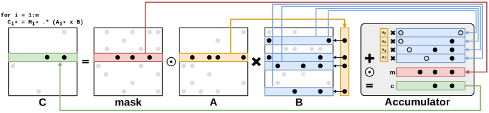
Figure 2. Row-wise Masked SpGEMM using an accumulator to compute output row $\mathbf{C}_{i*}$. The rows corresponding to the column indices of entries in row $\mathbf{A}_{i*}$ are merged and filtered through the respective mask entries to compute $\mathbf{C}_{i*}$. This merging and filtering process can be performed in a number of ways.

We describe four novel algorithms for Masked SpGEMM: Hash, Masked Sparse Accumulator (MSA), Mask Compressed Accumulator (MCA), and Heap. Three of these algorithms –Hash, MSA, and Heap– are novel improvements to the SpGEMM algorithms described in (deveci2018multithreaded, ; nagasaka2019performance, ; buluc2008representation, ), whereas MCA, to the best of our knowledge, is a completely new algorithm specifically developed for Masked SpGEMM. All algorithms belong to the category of row-by-row push-based algorithms (Section 4.2). The computational flow of row-by-row Masked SpGEMM algorithms is illustrated Figure 2. Each row $\mathbf{C}_{i*}$ is calculated as element-wise multiplication of $\mathbf{M}_{i*}$ and linear combination of each row $\mathbf{B}_{k*}$ for which $\mathbf{A}_{ik}\neq 0$, i.e., $\mathbf{C}_{i*}=\mathbf{M}_{i*}\odot\sum_{\mathbf{A}_{ik}\neq 0}{\mathbf{A}_{ik}\mathbf{B}_{k*}}$. Notice that calculation of each row can be seen as a row vector-matrix multiplication (SpGEVM) followed by mask operation $\mathbf{v}^{\intercal}=\mathbf{m}^{\intercal}\odot\left(\mathbf{u}^{\intercal}\mathbf{B}\right)$. In order to simplify the algorithm explanations, without loss of generality, in this section we describe different algorithms for computing Masked SpGEVM. Extrapolating Masked SpGEVM algorithms to devise Masked SpGEMM algorithms is straightforward.

5.1. Accumulator

A key component in all the Masked SpGEVM algorithms is the accumulator, which is basically a data structure to merge scaled rows and can be considered as a set union operation. The design and the implementation of the accumulator has a significant impact on memory hierarchy behaviour and therefore on the performance of Masked SpGEVM, and is the key differentiating feature between our proposed algorithms, so a more detailed description of the accumulator warrants its own subsection. We describe the accumulator as a generic interface that can be implemented differently by using various data structures in order to generate an output vector $\mathbf{v}$ (i.e., a row of $\mathbf{C}$).

The accumulator accumulates products $\mathbf{u}_{k}\mathbf{B}_{kj}$ with the same column index $j$ and discards all the values $\mathbf{v}_{j}$ for which $\mathbf{v}_{j}=0$. In order to reduce the number of unnecessary operations, the accumulator can altogether skip calculating the products that will be discarded. That is, the accumulator may calculate only the products $\mathbf{u}_{k}\mathbf{B}_{kj}$ for which $\mathbf{m}_{j}\neq 0$. Consequently, a more complex data structure than the Sparse Accumulator of Gilbert et al. (gilbert1992sparse, ) is needed. In particular, an accumulator for Masked SpGEVM needs to be able to differentiate between three states: SET, ALLOWED, and NOTALLOWED.

Our accumulator interface contains three procedures:

• setAllowed(key) marks the values that should not be discarded and have the potential to be in the output matrix.

• insert(key, value) inserts a key-value pair into the accumulator. Since the value that is being inserted may be discarded, the insert procedure allows the second argument (value) to be a lambda function that will only be evaluated if the value it computes will not be discarded.

• remove(key) accumulates all previously inserted values with the specified key and returns the value of the corresponding key. If no values with the specified key were previously inserted, or if setAllowed is never called for the specified key, the procedure remove returns none. After the function remove is called, all values with the specified key are removed from the accumulator.

We next describe how the four accumulators implement this interface and how they are used to perform SpGEVM.

5.2. Masked Sparse Accumulator (MSA)

Internally, MSA uses two dense arrays, $values$ and $\mathit{states}$, each with $\mathit{ncols}(\mathbf{v})$ length. $\mathit{values}$ stores the accumulated values, and $\mathit{states}$ stores information about the state of the entries in $\mathit{values}$, which may be one in of three states NOTALLOWED, ALLOWED, and SET. Initially, all of them are in the NOTALLOWED state and the only valid transition from this state is to the ALLOWED state, which is achieved by setAllowed. insert changes the state from ALLOWED to SET. When key-value pair $(K,V)$ is inserted into the MSA, if key $K$ was previously marked as ALLOWED and if no values with key $K$ were previously inserted, the respective is updated as SET and $\mathit{values}_{\mathit{key}}$ is set to $V$. Otherwise, if key $K$ was previously marked as SET –meaning that some value with key $K$ was previously inserted– the value $V$ is accumulated with the previous result. remove returns the accumulated value with the specified key if the accumulated value was previously set and returns none otherwise. Figure 3 shows MSA state automaton.

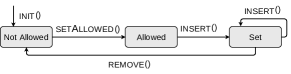
Figure 3. MSA states automaton

SpGEVM algorithm that uses MSA as accumulator is given in Algorithm 2 and has three main steps. First, the algorithm initializes MSA and by using the mask elements it marks the values in the MSA that should not be discarded as ALLOWED. Second, the algorithm finds all products $\mathbf{u}_{k}\mathbf{B}_{kj}$ for which $\mathbf{u}_{k}\neq 0$ and $\mathbf{B}_{kj}\neq 0$, and inserts them into MSA. Finally, the algorithm gathers all nonzero values from MSA, and resets the states in MSA. To improve the performance of this last gather operation, the algorithm only iterates over the entries that are present in the mask. Additionally, the values are gathered in the same order as they are ordered in the mask. This has the benefit of being stable: if, for example, the values in the mask are sorted by column indices, the values in the output vector $\mathbf{v}$ will also be sorted by column indices. Figure 4 shows masked SpGEVM algorithm that generates output vector $\mathbf{v}$ using MSA, where the mask acts a filter to determine which output entries are valid or invalid.

MSA algorithm can also be used if the mask is complemented. When the mask is complemented, the default state for the accumulator becomes ALLOWED, and for each element in the mask we invoke setNotAllowed instead of setAllowed. Additionally, if the mask is complemented we have an additional array to keep track of the elements that were inserted into the accumulator. This allows us to gather the accumulated values without iterating through the whole array. Similar strategy was used by Gustavson  (gustavson1978two, ).

MSA initialization takes $O(\mathit{ncols}(\mathbf{u}))$ operations, and computing the output vector $\mathbf{v}$ takes $O(\mathit{nnz}(\mathbf{m})+\mathit{flops}(\mathbf{u}\mathbf{B}))$ operations. Therefore, the algorithm takes $O(\mathit{ncols}(\mathbf{v})+\mathit{nnz}(\mathbf{m})+\mathit{flops}(\mathbf{u}\mathbf{B}))$ operations.

Algorithm 2 MSA Masked SpGEVM

1:Sparse row vectors $\mathbf{m}$, $\mathbf{u}$, and a sparse matrix $\mathbf{B}$

2:Sparse row vector $\mathbf{v}$

3:$accum\leftarrow\textsc{init}(ncols(\mathbf{B}))$

4:for each nonzero $\mathbf{m}_{j}$ in $\mathbf{m}$ do

5:    $accum.\textsc{setAllowed}(j)$

6:for each nonzero $\mathbf{u}_{k}$ in $\mathbf{u}$ do

7:    for each nonzero $\mathbf{B}_{kj}$ in row $\mathbf{B}_{k*}$ do

8:        $accum.\textsc{insert}(j,\lambda\rightarrow\mathbf{u}_{k}\mathbf{B}_{kj})$     

9:for each nonzero $\mathbf{m}_{j}$ in $\mathbf{m}$ do

10:    $value=accum.\textsc{remove}(j)$

11:    if $value\neq none$ then

12:        $\mathbf{v}_{j}\leftarrow value$     

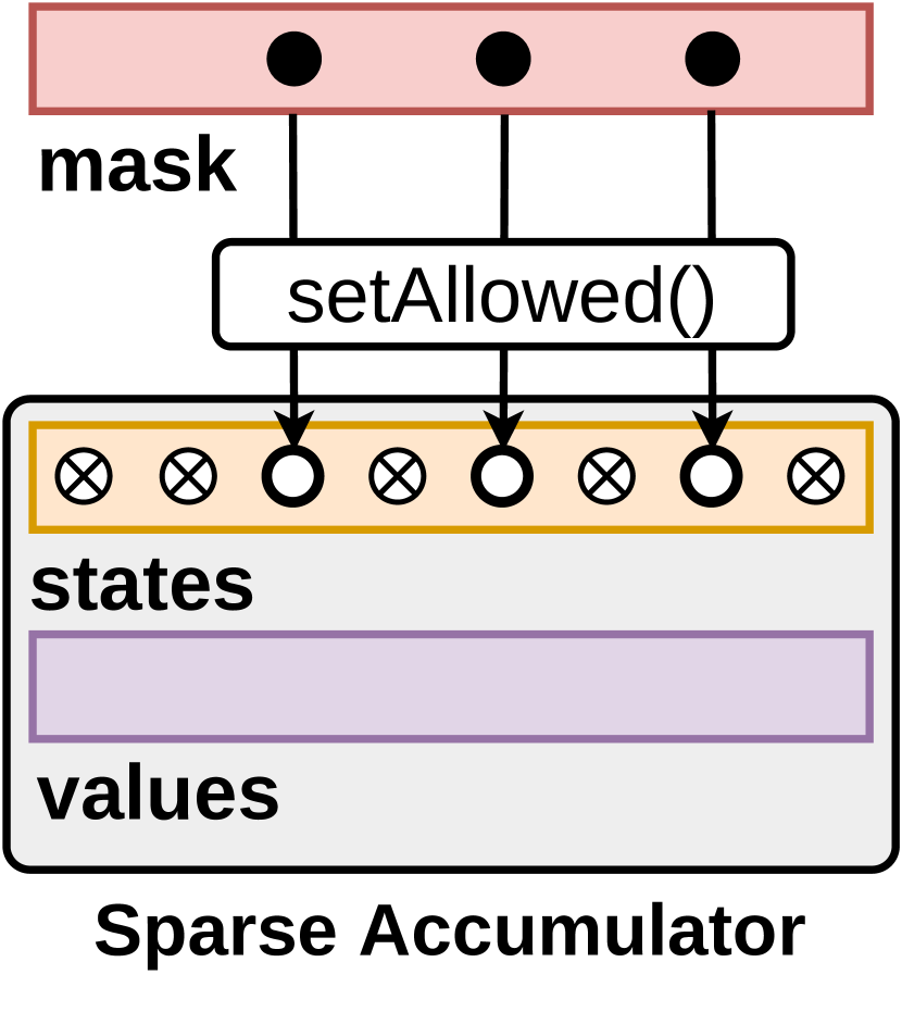
(a) Set allowed keys

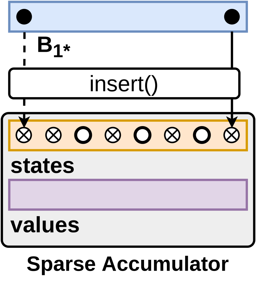
(b) MSA += $\mathbf{u}_{1}\times\mathbf{B}_{1*}$

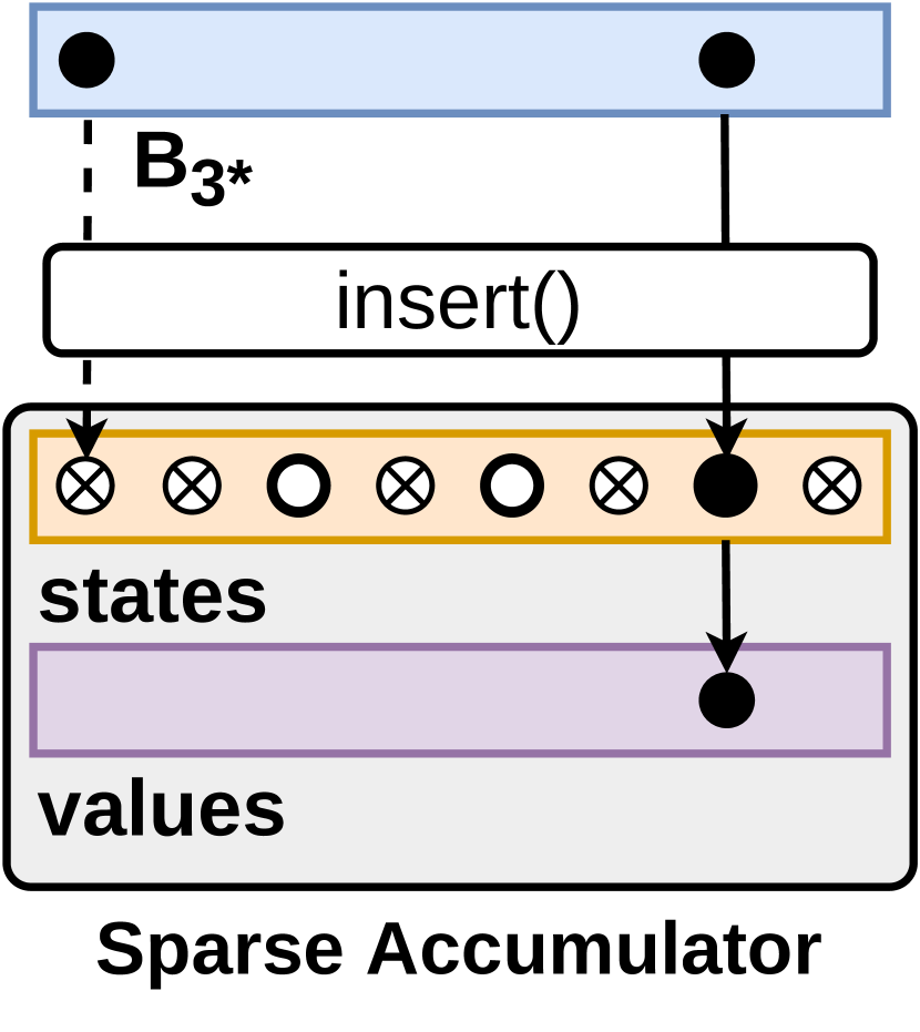
(c) MSA += $\mathbf{u}_{3}\times\mathbf{B}_{3*}$

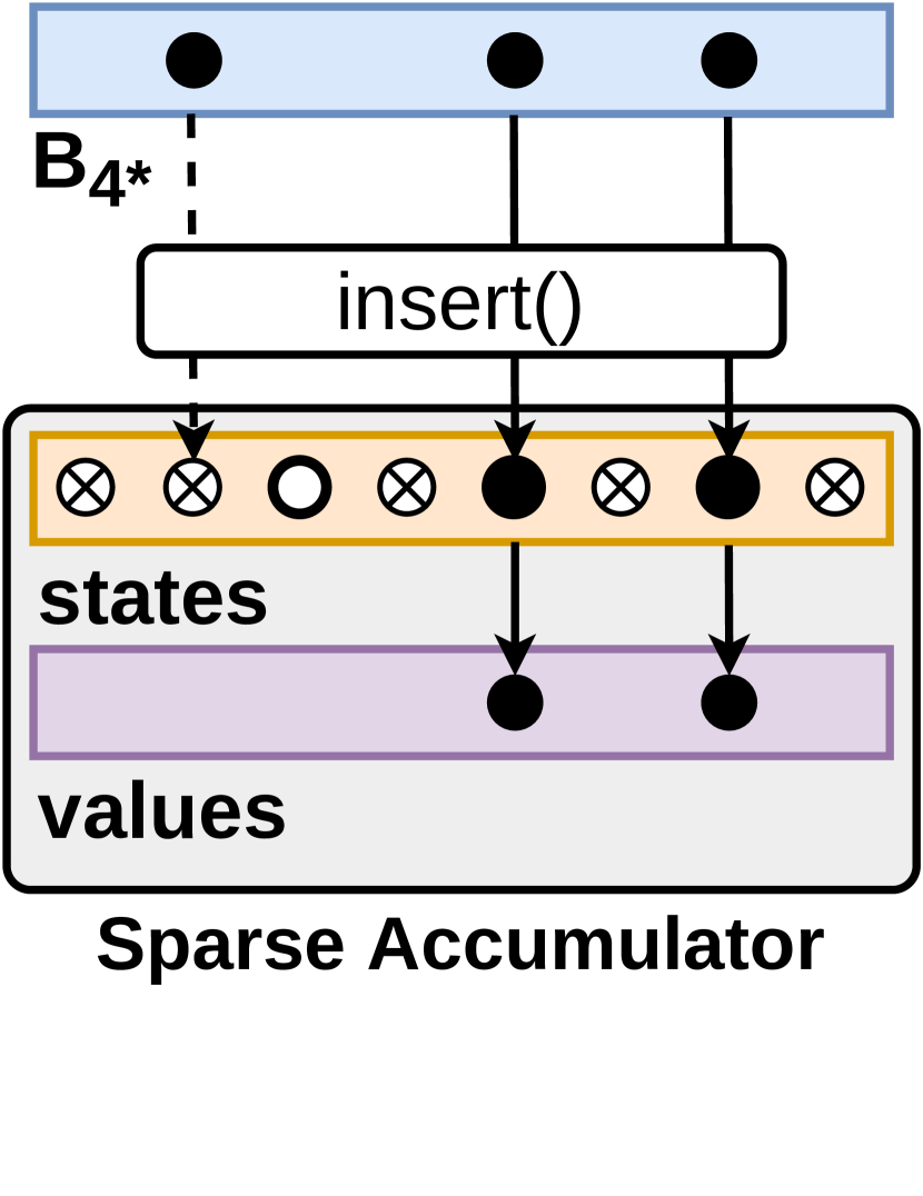
(d) MSA += $\mathbf{u}_{4}\times\mathbf{B}_{4*}$

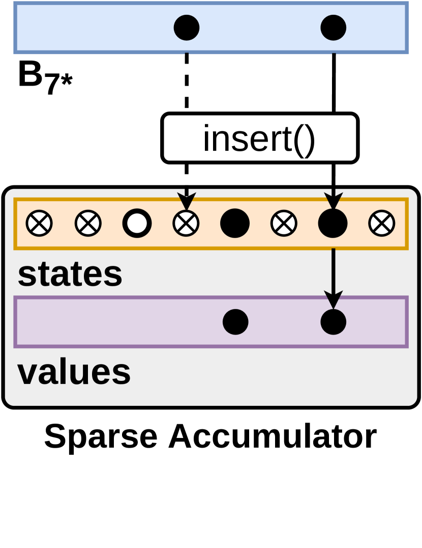
(e) MSA+= $\mathbf{u}_{7}\times\mathbf{B}_{7*}$

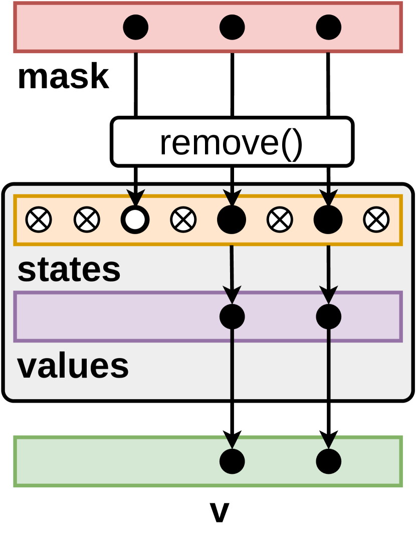
(f) Move values to $\mathbf{v}$

Figure 4. Masked SpGEVM algorithm using Masked Sparse Accumulator (MSA).

5.3. Hash Accumulator

In practice, the arrays in the MSA accumulator are too large to fit in L1 cache, even though they usually have only a few nonzeros, so indexing an element of these arrays usually incurs a cache miss in the MSA algorithm  (Patwary2015, ). To overcome this issue, we utilize a hash map instead of dense arrays for storing values and states, reducing cache misses but increasing access overhead. To reduce the hash accesses, we store both the accumulated value and its state as a pair in one single hash map, using open addressing with linear probing, no resizing support since we know it will have $\mathit{nnz}(\mathbf{m})$ values, and a load factor of $0.25$ to reduce collisions. Others (nagasaka2019performance, ; deveci2018multithreaded, ) use similar hash accumulators for plain SpGEMM.

The time complexity of SpGEVM is $O(\mathit{nnz}(\mathbf{m})+\mathit{flops}(\mathbf{u}\mathbf{B}))$ operations, since initialization does not depend on $\mathit{ncols}(\mathbf{v})$ but on the number of nonzeros in mask $\mathbf{m}$. Hash accumulator has a smaller memory footprint than MSA, but accessing individual values requires computing the hash.

5.4. Mask Compressed Accumulator (MCA)

Mask Compressed Accumulator (MCA) algorithm is based on the observation that the number of elements in the accumulator cannot be greater than the number of nonzeros in mask $\mathbf{m}$. The MCA accumulator uses size $nnz(\mathbf{m})$ for the $values$ and $states$ arrays. The previously described MSA and Hash algorithms use column indices to index the accumulator. However, column indices cannot be used to index the MCA accumulator because $\mathit{ncols}(\mathbf{B})$ is greater than or equal to $\mathit{nnz}(\mathbf{m})$, i.e., the length of the arrays in the MCA accumulator. Therefore, we need another way to index the MCA accumulator. Since the indices should be in range $[0,\mathit{nnz}(\mathbf{m}))$, when we have a nonzero element in mask with index $j$, and when $\mathbf{u}_{k}\neq 0\ \mathrm{and}\ \mathbf{B}_{kj}\neq 0$, we can use the number of nonzero elements in $\mathbf{m}_{j}$ with column index smaller than $j$. The MCA accumulator needs only two states ALLOWED and SET because by relying on the mask elements, it readily ensures no key can be in NOTALLOWED state. Figure  5 shows MCA state automaton algorithm and Figure 6(e) shows masked SpGEVM algorithm that generates output vector $\mathbf{v}$ using MCA.

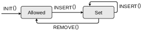
Figure 5. MCA states automaton

For sorted input, the index for the MCA accumulator can be calculated quickly. For each nonzero in $\mathbf{u}$ the algorithm iterates through $\mathbf{m}$ at most once, and it accesses the entries in $\mathbf{B}_{k*}$ once for which $\mathbf{u}_{k}\neq 0$ and $\mathbf{B}_{kj}\neq 0$. Hence, the algorithm takes $O(\mathit{nnz}(\mathbf{u})\cdot\mathit{nnz}(\mathbf{m})+\mathit{flops}(\mathbf{u}\mathbf{B}))$ time.

Algorithm 3 MCA Masked SpGEVM

1:Sparse row vectors $\mathbf{m}$, $\mathbf{u}$, and a sparse matrix $\mathbf{B}$

2:Sparse row vector $\mathbf{v}$

3:$accum\leftarrow\textsc{init}(nnz(\mathbf{m}))$

4:for each nonzero $\mathbf{u}_{k}$ in $\mathbf{u}$ do

5:    $rowIter\leftarrow MakeIterator(\mathbf{B}_{k*})$

6:    for each $(idx,\mathbf{m}_{j})$ in $Enumerate(\mathbf{m})$ do

7:        while $rowIter\land rowIter.colId<j$ do

8:           $rowIter\leftarrow Next(rowIter)$         

9:        if $rowIter\land rowIter.colId=j$ then

10:           $accum.\textsc{insert}(idx,\mathbf{u}_{k}\mathbf{B}_{kj})$             

11:for each $(idx,\mathbf{m}_{j})$ in $Enumerate(\mathbf{m})$ do

12:    $value=accum.\textsc{remove}(idx)$

13:    if $value\neq none$ then

14:        $\mathbf{v}_{j}\leftarrow value$     

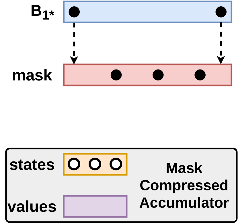
(a) $\textrm{MCA}=\mathbf{u}_{1}\times\mathbf{B}_{1*}$

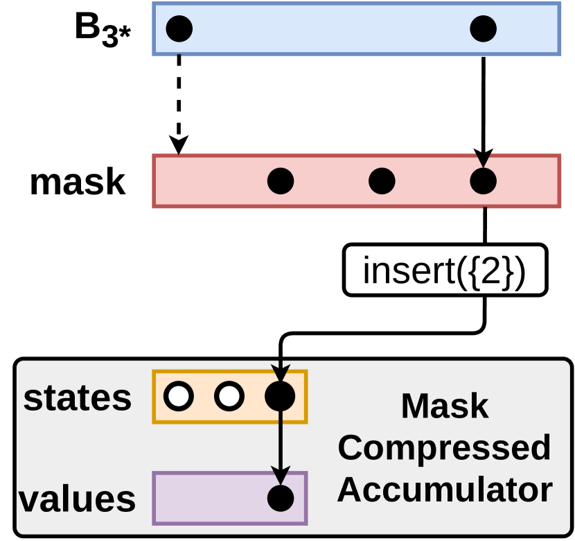
(b) $\textrm{MCA}+=\mathbf{u}_{3}\times\mathbf{B}_{3*}$

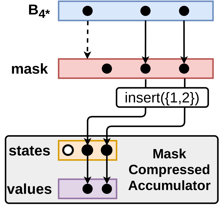
(c) $\textrm{MCA}+=\mathbf{u}_{4}\times\mathbf{B}_{4*}$

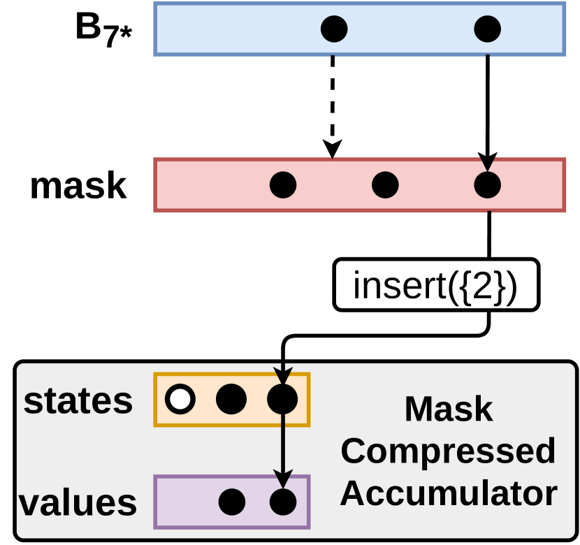
(d) $\textrm{MCA}+=\mathbf{u}_{7}\times\mathbf{B}_{7*}$

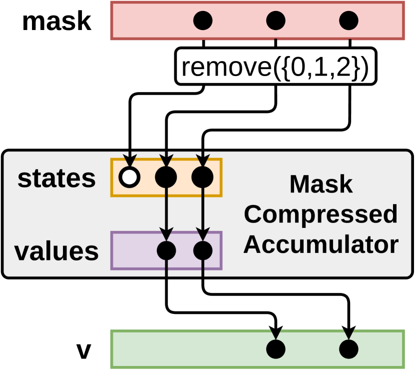
(e) Moving the result to $\mathbf{v}$

Figure 6. Masked SpGEVM algorithm using Mask Compressed Accumulator (MCA)

.

5.5. Masked Heap SpGEVM Algorithm

In this section we describe a Masked SpGEVM algorithm based on column-column Heap algorithm developed by Buluç and Gilbert (buluc2008representation, ). Like the base algorithm, our heap algorithm requires that the indices in mask $\mathbf{m}$ and column indices in matrix $\mathbf{B}$ are sorted. To compute the output vector $\mathbf{v}$, our algorithm uses a min-heap (or a priority queue). The heap initially contains $\mathit{nnz}(\mathbf{u})$ row iterators that point to the first element of rows $\{\mathbf{B}_{k*}$ | $\mathbf{u}_{k}\neq 0\}$. The iterators in the heap are ordered based the column index of the element they point to. By popping the top iterator from the heap, incrementing it, and pushing the incremented iterator back to the heap, we can iterate through set $\mathbf{S}=\{\mathbf{B}_{kj}|\mathbf{u}_{k}\neq 0\}$ in sorted order without having to construct the sorted set in memory. This is similar to the multi-way merge from (10.5555/280635, ). Since the indices in mask $\mathbf{m}$ are also sorted, we can easily find the intersection between the mask and set $\mathbf{S}$ by performing a 2-way merge. For all elements $\mathbf{B}_{kj}$ that belong to the intersection, the algorithm calculates $\mathbf{u}_{k}\mathbf{B}_{kj}$ products and inserts the result to the output. If the last inserted product has the same column index as the product currently being inserted, the result of the current product is added to the last product. Otherwise, a new entry is added to the output. Algorithm 4 shows the pseudo-code for the masked heap SpGEVM algorithm and Algorithm 5 shows the insert procedure for the heap.

The heap iterates through the mask, and pops $\mathit{flops}(\mathbf{u}\mathbf{B})$ elements from the heap. The complexity of the algorithm is $O(\mathit{nnz}(\mathbf{m})+\log_{2}\mathit{nnz}(\mathbf{u})\cdot\mathit{flops}(\mathbf{u}\mathbf{B}))$, since the maximum heap size is $\mathit{nnz}(\mathbf{u})$. Compared to MSA and Masked Hash algorithm, heap algorithm has smaller memory footprint but greater asymptotic complexity due to the logarithmic factor. To alleviate this, we can exploit the fact that only the elements in the intersection $\mathbf{m}\cap\mathbf{S}$ will be used to form the output and we can check whether the element will be a part of the intersection before we push it to the heap. Such a check might require us to iterate through the whole mask. For this reason, we configure the algorithm to inspect only a portion of the mask $\mathbf{m}$ before pushing an element to the heap by using the NInspect parameter (Algorithm 5), which controls the length of the portion of the mask to be checked. If this parameter is 0, the algorithm is identical to the algorithm described earlier. If it is 1, the algorithm inspects only the current mask element and has complexity $O(\mathit{nnz}(\mathbf{m})+(\alpha+(1-\alpha)\cdot\log_{2}\mathit{nnz}(\mathbf{u}))\cdot\mathit{flops}(\mathbf{u}\mathbf{B}))$, where $\alpha$ depends on the input and $\alpha\in[0,1]$. In our experiments we test 1 and $\infty$ for the NInspect parameter.

For mask complement, the only difference is that instead of computing $\mathbf{u}_{k}\mathbf{B}_{kj}$ products for the elements in intersection $\mathbf{m}\cap\mathbf{S}$, we compute the products for the elements in set difference $\mathbf{S}\setminus\mathbf{m}$. When mask is complemented, NInspect parameter is always 0.

Algorithm 4 Heap Masked SpGEVM

1:Sparse row vectors $\mathbf{m}$, $\mathbf{u}$, and a sparse matrix $\mathbf{B}$

2:Sparse row vector $\mathbf{v}$

3:$mIter\leftarrow MakeIterator(\mathbf{m})$

4:for each $\mathbf{u}_{k}$ in $\mathbf{u}$ do

5:    $\textsc{insert}(PQ,MakeIterator(\mathbf{B}_{k*}),mIter)$

6:$prevKey\leftarrow none$

7:while $\neg PQ.isEmpty()$ do

8:    $minIter\leftarrow PQ.popMin()$

9:    while $mIter\land mIter.colId<minIter.colId$ do

10:        $mIter\leftarrow Next(mIter)$     

11:    if $\neg mIter$ then

12:        break     

13:    if $mIter.colId=minIter.colId$ then

14:        $k\leftarrow minIter.rowId$

15:        $j\leftarrow minIter.colId$

16:        if $prevKey=minIter.colId$ then

17:           $\mathbf{v}_{j}\leftarrow\mathbf{v}_{j}+\mathbf{u}_{k}\mathbf{B}_{kj}$ $\triangleright$ $\mathbf{v}_{j}$ is the last value in $\mathbf{v}$

18:        else

19:           $prevKey\leftarrow minIter.colId$

20:           $\mathbf{v}_{j}\leftarrow\mathbf{u}_{k}\mathbf{B}_{kj}$ $\triangleright$ $\mathbf{v}_{j}$ is the last value in $\mathbf{v}$             

21:    $\textsc{insert}(PQ,Next(minIter),mIter)$

Algorithm 5 Insert procedure for Heap Masked SpGEVM

1:procedure Insert(PQ, rowIter, mIter, NInspect)

2:    if $\neg IsValid(rowIter)$ then

3:        return     

4:    if $NInspect=0$ then

5:        $PQ.insert(rowIter)$;

6:        return     

7:    $toInspect\leftarrow NInspect$

8:    while $IsValid(rowIter)\land IsValid(mIter)$ do

9:        if $rowIter.colId=mIter.colId$ then

10:           $PQ.insert(rowIter)$;

11:           return

12:        else if $rowIter.colId<mIter.colId$ then

13:           $rowIter\leftarrow Next(rowIter)$

14:        else

15:           $mIter\leftarrow Next(mIter)$

16:           $toInspect\leftarrow toInspect-1$

17:           if $toInspect=0$ then

18:               $PQ.insert(rowIter)$;

19:               return                        

6. Symbolic and Numeric Phases

The size and the pattern of the output matrix in the Masked SpGEMM are not known before the multiplication. To allocate the needed space and form the output matrix, there are two methods: one-phase and two-phase approaches.

In the one-phase approach, the Masked SpGEMM is performed all at once, first allocating temporary memory large enough to store the output matrix, executing the Masked SpGEMM, and then copy the values from the temporary memory to the output matrix. This is often deemed inefficient in plain SpGEMM, especially when the compression factor is large. However, mask can provide a good initial approximation for the size of the output matrix, making one-phase approaches more viable for Masked SpGEMM.

In the two-phase approach, we first execute a symbolic multiplication that only inspects the row and column indices from the inputs to computes the number of nonzeros in the output matrix, then allocate memory for the output matrix and execute the actual multiplication. The former is known as the symbolic and the latter is known as the numeric phase.

The trade-off between these two approaches is in memory footprint vs. amount of computation. The two-phase approach reduces the memory footprint at the expense of increased computation. We evaluate both approaches for the algorithms described in our work since the addition of the mask to the multiplication has the potential to alter the balance between these trade-offs for plain SpGEMM.

7. Experimental Setup

We conduct our experiments on both synthetic and real-world graphs. The synthetic graphs are preferred for controlled experiments in which we vary degree or size of the graphs and investigate their effects on various performance metrics. For the synthetic graphs, we utilize Erdős-Rényi graphs as well as graphs generated with R-MAT generator (Chakrabarti2004, ), with parameters identical to those used in the Graph500 benchmark (murphy2010introducing, ). For real-world graphs, we use the same set of 26 graphs that Nagasaka et al. (nagasaka2019performance, ) (Table 2 of the referenced paper) used, which are all from SuiteSparse Matrix Collection (Davis2011, ). Since we only plot performance profiles (Dolan2002, ) where we report on the fraction of input cases as a function of the relative runtime of each algorithm, we do not repeat the graph properties here. Their input nonzeros range from $350$K to $100$M.

We conduct our experiments on two different systems: Haswell with Intel Xeon E5-2698 processors (two sockets per node, 2.3 GHz, 32 total cores, 128GB) and KNL with Intel Xeon Phi 7250 processors (one socket per node, 1.4 GHz, 68 cores, 96 GB). All algorithms are implemented in C++, compiled with gcc v10.1 with -O3 flag. Threads are pinned to cores using GOMP_CPU_AFFINITY. As a baseline, we use SuiteSparse:GraphBLAS version 5.1.4 compiled with the same parameters as above. With the exception of scaling experiments, we use 32 threads on Haswell and 68 threads on KNL in all experiments.

We benchmark three different applications on real-world graphs: (i) Triangle Counting, (ii) $k$-truss, and (iii) Betweenness Centrality. Triangle Counting computes the total number of triangles in a graph, using one Masked SpGEMM operation along with a reduction. $k$-truss finds the edges that are supported by at least $k$-2 other edges, using Masked SpGEMM in an iterative manner where the the graph keeps changing due to pruning of some edges. The Betweenness Centrality measures how central is a node in the graph by computing the ratio of shortest paths that node is on (Freeman1977, ), using a multi-source two-stage algorithm (Brandes2001, ). All these algorithms are implemented within the GraphBLAS specifications, substituting Masked SpGEMM operations with calls to different algorithms investigated in this work to measure their performance.

8. Experimental Results

In this section we compare several algorithms on three benchmarks: Triangle Counting, $k$-truss, and Betweenness Centrality. We evaluated the following schemes: Inner (pull-based inner-product-parallel algorithm from Section 4.1), MSA (push-based algorithm using masked sparse accumulator from Section 5.2), Hash (push-based algorithm using hash accumulator from Section 5.3), MCA (push-based algorithm using compressed mask accumulator from Section 5.4), Heap (push-based algorithm using a heap accumulator with $NInspect=1$ from Section 5.5), HeapDot (push-based algorithm using a heap accumulator with $NInspect=\infty$ from Section 5.5), and two variants of Masked SpGEMM from SuiteSparse:GraphBLAS (Davis2019, ) (SS:GB) library: SS:DOT, a pull-based algorithm similar to Inner, and SS:SAXPY, a push-based algorithm that, depending on the problem, can use SPA-like data structure or a hash table to accumulate values.

Each of our algorithms can be executed with and without a symbolic phase, which are respectively indicated with suffixes 2P and 1P. In total, we evaluate 14 algorithms, 10 of which are proposed in this work, 2 are based on the previous work (yang2019graphblast, ), and 2 of them from SS:GB are used as baseline.

8.1. Effect of Input Matrix and Mask Density

In this section we investigate the performance of our Masked SpGEMM algorithms with changing mask and input matrix density. These experiments are conducted on Haswell. Figure 7 plots the best performing algorithm for multiple different Erdős-Rényi inputs by varying the degree of the mask in $x$ axis and the degrees of the input matrices in $y$ axis.

When mask is much sparser than $\mathbf{A}$ and $\mathbf{B}$, Inner has the best performance, which is because Inner is able to avoid a great amount of unnecessary operations that the other algorithms suffer from. When $\mathbf{A}$ and $\mathbf{B}$ are much sparser than mask, on the other hand, Heap and HeapDot perform the best. In all other cases where mask and input matrix density are comparable, MSA and Hash show the best performance, with MSA performing better on smaller matrices and Hash on larger ones – which can be attributed to MSA’s worsening cache utilization as the matrices get larger.

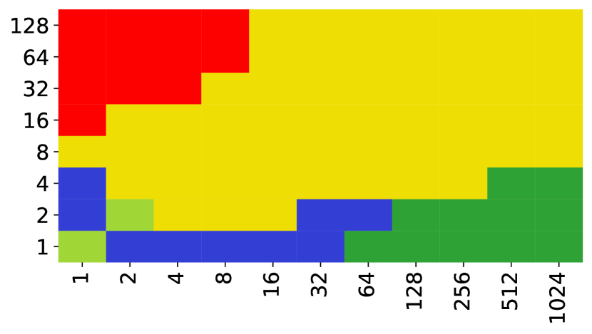
(a) dimension = $2^{12}\times 2^{12}$

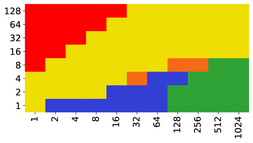
(b) dimension = $2^{14}\times 2^{14}$

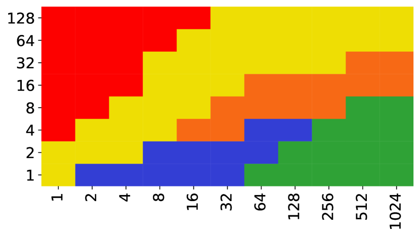
(c) dimension = $2^{16}\times 2^{16}$

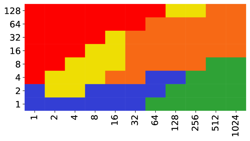
(d) dimension = $2^{18}\times 2^{18}$

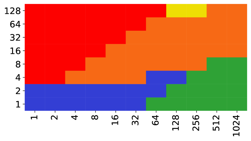
(e) dimension = $2^{20}\times 2^{20}$

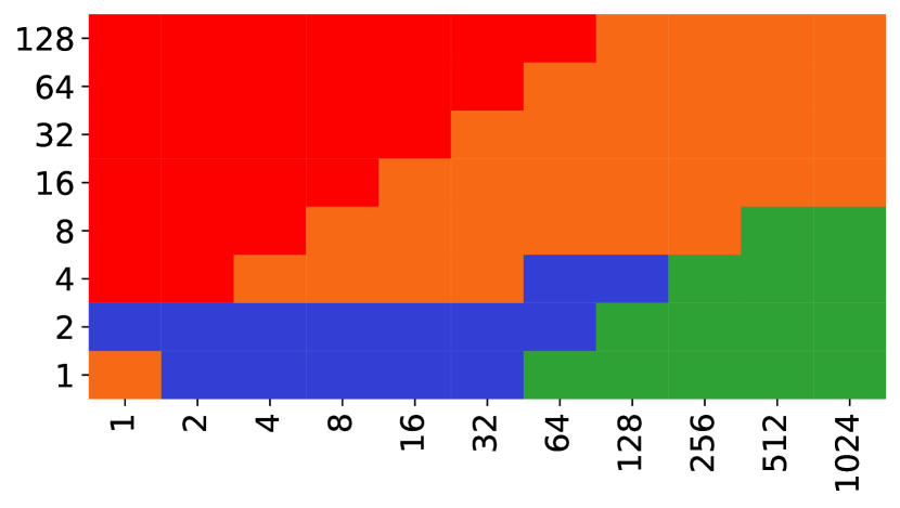
(f) dimension = $2^{22}\times 2^{22}$

Figure 7. The best performing schemes with varying input and mask density.

8.2. Triangle Counting

We next benchmark performance all schemes on Triangle Counting benchmark. For optimal performance, vertices in the original graph should be sorted in non-increasing order of their degrees (lumsdaine2020triangle, ). After relabeling, the number of triangles is given by as $sum(\mathbf{L}.*(\mathbf{L}^{2}))$, where $\mathbf{L}$ is the lower triangular matrix. This method is known to be among the fastest ways to compute Triangle Counting (Davis2018, ). In our experiments, we only report the Masked SpGEMM execution time.

Relative Performance of Masked SpGEMM Algorithms. Figure 8 shows the performance profiles of all our algorithms tested on all real graphs. In the performance profile plots (Dolan2002, ), a point $(x,y)$ indicates that the scheme for that point is within $x$ factor of the best obtained result in $y$ fraction of the test cases. The closer a scheme’s line is to the $y$ axis, the better is its performance.

In this benchmark, the best performing scheme is MSA-1P, outperforming all other algorithms for 65% of the test cases, followed by MCA-1P. These are followed by Inner and Hash schemes, with Heap and HeapDot being the worst. Observe that the one-phase variant of each algorithm performs better than than its two-phase variant. We exclude two-phase variants and heap-based schemes from our discussions in this section to keep our plots more readable.

Figure 9 compares the performance of our three best performing algorithms against the SS:GB algorithms. We can see that all our algorithms outperform SS:GB algorithms in almost all cases. Performance profiles are almost identical on KNL and excluded due to space.

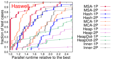
Figure 8. Triangle Counting: our algorithms

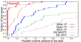
Figure 9. Triangle Counting: our algorithms vs. SS:GB.

Scaling with Input Size. Figure 10 shows the performance on Haswell and KNL for R-MAT matrices with scale ranging from 8 to 20. MSA-1P obtains the highest GFLOPS rates on both KNL and Haswell. Hash-1P and MCA-1P are slower than MSA-1P but they have similar trends. SS:GB algorithms have bad performance for small inputs, however, as input size increases, SS:SAXPY gets closer to MSA-1P.

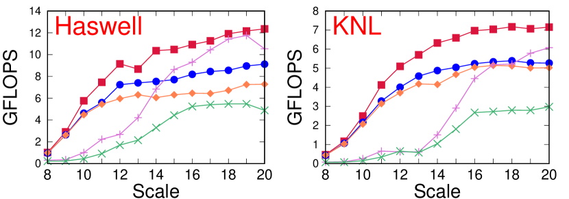
Figure 10. Triangle Counting: varying R-MAT scale.

Scaling with Thread Count. Figure 11 shows the scalability analysis on Haswell and KNL for R-MAT matrix with scale 20, on up to 32 threads on Haswell, and up to 68 threads on KNL, with all algorithms scaling well in all cases.

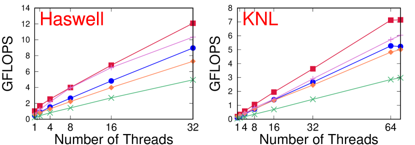
Figure 11. Triangle Counting: strong scaling (varying thread count) on R-MAT scale 20.

8.3. $k$-truss

For $k$-truss benchmark, we use $k=5$ and report the sum of flops required to perform all Masked SpGEMM operations divided by total time required to execute them.

Relative Performance of Masked SpGEMM Algorithms. Figure 12 shows the performance of all our algorithms on all real graphs except wb-edu (excluded for its long running time).

MSA performs the best on Haswell while Inner performs fairly well on both, likely due to the mask getting sparser as $k$-truss prunes the graph more with each iteration. MSA’s better performance on Haswell can be attributed to the existence of a large L3 cache (40 MB, whereas KNL has no L3 cache), hiding the cache misses due to large accumulator arrays in MSA to an extent. The 1P schemes again perform better than 2P. Heap-based methods are noncompetitive, so we exclude them from our plots in the rest of this section.

Figure 13 compares the performance of our four best performing algorithms against the SS:GB algorithms. Our schemes MSA-1P and Inner-1P perform significantly better than SS:GB schemes on Haswell and KNL, respectively.

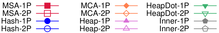
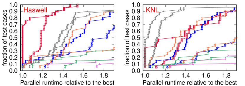
Figure 12. $k$-truss: Performance of the proposed schemes

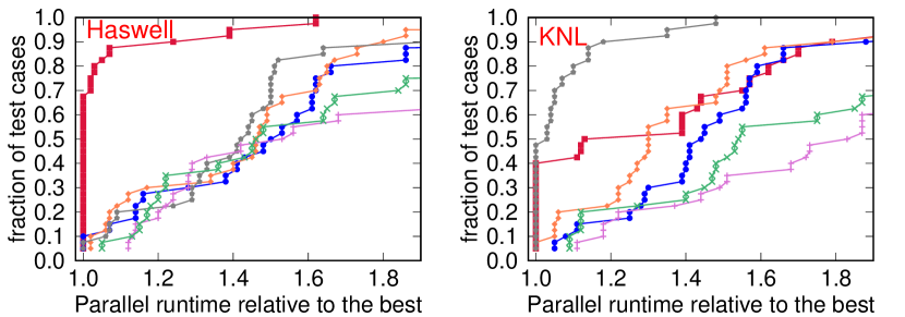
Figure 13. $k$-truss: our algorithms vs. SS:GB

Scaling with Input Size. Figure 14 shows the algorithm performance on Haswell and KNL for R-MAT matrices with scale ranging from 8 to 20. Inner and SS:DOT increase their GFLOPS rate well with increasing matrix scale, while MSA-1P does this only on Haswell. The pull-based algorithms seem to attain better GFLOPS rates in the $k$-truss benchmark. This benchmark shows that the algorithms that are deemed inefficient for plain SpGEMM can attain quite good performance when mask becomes part of the multiplication and can lead to highest GFLOPS rates.

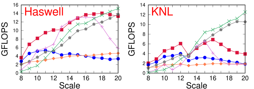
Figure 14. $k$-truss: varying R-MAT scale.

8.4. Betweenness Centrality

Betweenness Centrality consists of a forward and backward stage, and uses both a complemented and non-complemented Masked SpGEMM. For this benchmark, we use TEPS (bader2006hpcs, ), which is $\textit{batch\_size}\times\textit{num\_edges}/\textit{total\_time}$ as performance metric. We use a batch size of 512.

Relative Performance of Masked SpGEMM Algorithms. Figure 16 shows the performance of all our algorithms on all real graphs except cage15, delaunay_n24, and wb-edu (excluded for their long running time). We benchmarked the Masked SpGEMM in forward and backward stages separately, but the trends were similar so we only present the overall performance. MCA is not included in these results because it does not support complemented Masked SpGEMM. We excluded Heap, Inner, and SS:DOT since they were prohibitively slow.

In this benchmark, MSA-1P obtains the best performance in all test instances. 1P schemes again outperform 2P.

Scaling with Input Size. Figure 11 shows the algorithm performance on Haswell and KNL for R-MAT matrices with scale ranging from 8 to 20. The schemes based on push-based algorithms, i.e., MSA-1P, Hash-1P, and SS:SAXPY are able increase their MTEPS rate with increasing matrix scale. The mask in Betwenness Centrality can get quite dense, so the poor cache utilization of SS:DOT becomes a very serious bottleneck. In addition, the matrix $\mathbf{B}$ is transposed in the library before each Masked SpGEMM, increasing overhead.

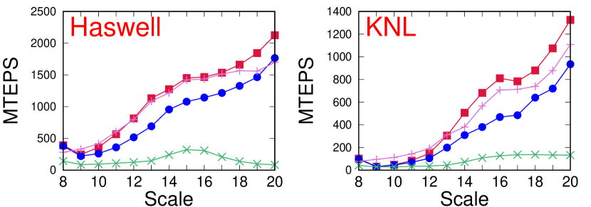
Figure 15. Betweenness Centrality: varying R-MAT scale.

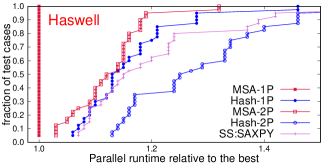
Figure 16. Betweenness Centrality: our schemes vs. SS:GB.

9. Conclusions and Future Work

In this paper, we presented four novel algorithms (with 10 total variations) for performing parallel masked sparse-sparse matrix multiplication.

We investigated Masked SpGEMM operation from various design and optimization standpoints to evaluate whether the challenges posed for plain SpGEMM still hold, and examined if some of the uncommon design choices can be reevaluated when mask is part of the multiplication. We discovered that the mask and matrix density both have a critical effect on the performance of different design choices. Surprisingly, we discovered that inner-product-based algorithm can be competitive in certain benchmarks with high mask sparsity on systems with small cache size. We have shown that computing the Masked SpGEMM in a single phase usually performs better than approaches in which a symbolic multiplication is run prior to actual multiplication, in stark contrast with the conventions of plain SpGEMM computations where two-phase approaches are often more preferable. We ran extensive experiments on two very different machines, with large sets of matrices, on several real-world benchmarks, and demonstrated that in almost all cases our methods significantly outperform the SuiteSparse:GraphBLAS (Davis2019, ) library, which is, to the best of our knowledge, the fastest Masked SpGEMM implementation in existence to-date.

As future work, we will investigate hybrid algorithms that can use different accumulators in the same Masked SpGEMM depending on the density of the mask and parts of matrices being processed, as well as exploiting fine-grain parallelism within single row processing.

- [1] Ariful Azad, Grey Ballard, Aydın Buluç, James Demmel, Laura Grigori, Oded Schwartz, Sivan Toledo, and Samuel Williams. Exploiting multiple levels of parallelism in sparse matrix-matrix multiplication. SIAM Journal on Scientific Computing, 38(6):C624–C651, 2016.
- [2] Ariful Azad, Aydin Buluç, and John Gilbert. Parallel triangle counting and enumeration using matrix algebra. In International Parallel and Distributed Processing Symposium Workshops, pages 804–811. IEEE, 2015.
- [3] Mohsen Aznaveh, Jinhao Chen, Timothy A Davis, Bálint Hegyi, Scott P Kolodziej, Timothy G Mattson, and Gábor Szárnyas. Parallel GraphBLAS with OpenMP. In Proceedings of the SIAM Workshop on Combinatorial Scientific Computing, pages 138–148. SIAM, 2020.
- [4] David A Bader, John Feo, John Gilbert, Jeremy Kepner, David Koester, Eugene Loh, Kamesh Madduri, Bill Mann, and Theresa Meuse. HPCS scalable synthetic compact applications 2: graph analysis. SSCA, 2:v2, 2006.
- [5] Scott Beamer, Krste Asanovic, and David Patterson. Direction-optimizing breadth-first search. In SC’12: Proceedings of the International Conference on High Performance Computing, Networking, Storage and Analysis, pages 1–10. IEEE, 2012.
- [6] Nathan Bell, Steven Dalton, and Luke N. Olson. Exposing fine-grained parallelism in algebraic multigrid methods. SIAM Journal on Scientific Computing, 34(4):C123–C152, 2012.
- [7] Maciej Besta, Michał Podstawski, Linus Groner, Edgar Solomonik, and Torsten Hoefler. To push or to pull: On reducing communication and synchronization in graph computations. In Proceedings of the 26th International Symposium on High-Performance Parallel and Distributed Computing, pages 93–104, 2017.
- [8] Ulrik Brandes. A faster algorithm for betweenness centrality. The Journal of Mathematical Sociology, 25(2):163–177, 2001.
- [9] W. Briggs, V. Henson, and S. McCormick. A Multigrid Tutorial, Second Edition. Society for Industrial and Applied Mathematics, second edition, 2000.
- [10] Aydin Buluc and John R Gilbert. On the representation and multiplication of hypersparse matrices. In IEEE International Symposium on Parallel and Distributed Processing, pages 1–11. IEEE, 2008.
- [11] Aydin Buluç, Tim Mattson, Scott McMillan, José Moreira, and Carl Yang. Design of the GraphBLAS API for C. In International Parallel and Distributed Processing Symposium Workshops (IPDPSW), pages 643–652. IEEE, 2017.
- [12] Aydin Buluç and John R. Gilbert. Parallel sparse matrix-matrix multiplication and indexing: Implementation and experiments. SIAM Journal on Scientific Computing, 34(4):C170–C191, 2012.
- [13] Deepayan Chakrabarti, Yiping Zhan, and Christos Faloutsos. R-MAT: A Recursive Model for Graph Mining, pages 442–446.
- [14] Timothy A Davis. Algorithm 10xx: Suitesparse:graphblas: parallel graph algorithms in the language of sparse linear algebra. draft manuscript.
- [15] Timothy A. Davis. Graph algorithms via suitesparse: Graphblas: triangle counting and k-truss. In 2018 IEEE High Performance extreme Computing Conference (HPEC), pages 1–6, 2018.
- [16] Timothy A. Davis. Algorithm 1000: Suitesparse:graphblas: Graph algorithms in the language of sparse linear algebra. ACM Trans. Math. Softw., 45(4), December 2019.
- [17] Timothy A Davis and Yifan Hu. The university of florida sparse matrix collection. ACM Trans. Math. Softw. (TOMS), 38(1):1–25, 2011.
- [18] Mehmet Deveci, Christian Trott, and Sivasankaran Rajamanickam. Performance-portable sparse matrix-matrix multiplication for many-core architectures. In IEEE International Parallel and Distributed Processing Symposium Workshops (IPDPSW), pages 693–702, 2017.
- [19] Mehmet Deveci, Christian Trott, and Sivasankaran Rajamanickam. Multithreaded sparse matrix-matrix multiplication for many-core and gpu architectures. Parallel Computing, 78:33–46, 2018.
- [20] Elizabeth D. Dolan and Jorge J. Moré. Benchmarking optimization software with performance profiles. Mathematical Programming, 91(2):201–213, Jan 2002.
- [21] Philip A Etter, Kai Zhong, Hsiang-Fu Yu, Lexing Ying, and Inderjit Dhillon. Accelerating inference for sparse extreme multi-label ranking trees. arXiv preprint arXiv:2106.02697, 2021.
- [22] Linton C. Freeman. A set of measures of centrality based on betweenness. Sociometry, 40(1):35–41, 1977.
- [23] John R Gilbert, Cleve Moler, and Robert Schreiber. Sparse matrices in MATLAB: Design and implementation. SIAM Journal on Matrix Analysis and Applications, 13(1):333–356, 1992.
- [24] John R. Gilbert, Steve Reinhardt, and Viral B. Shah. A unified framework for numerical and combinatorial computing. Computing in Science Engineering, 10(2):20–25, 2008.
- [25] Andreas Griewank and Uwe Naumann. Accumulating jacobians as chained sparse matrix products. Mathematical Programming, 95(3):555–571, Mar 2003.
- [26] Fred G Gustavson. Two fast algorithms for sparse matrices: Multiplication and permuted transposition. ACM Transactions on Mathematical Software (TOMS), 4(3):250–269, 1978.
- [27] Donald E. Knuth. The Art of Computer Programming, Volume 3: (2nd Ed.) Sorting and Searching. Addison Wesley Longman Publishing Co., Inc., USA, 1998.
- [28] W. Liu and B. Vinter. An efficient gpu general sparse matrix-matrix multiplication for irregular data. In IEEE 28th International Parallel and Distributed Processing Symposium, pages 370–381, May 2014.
- [29] Andrew Lumsdaine, Luke Dalessandro, Kevin Deweese, Jesun Firoz, and Scott McMillan. Triangle counting with cyclic distributions. In 2020 IEEE High Performance Extreme Computing Conference (HPEC), pages 1–8. IEEE, 2020.
- [30] Richard C Murphy, Kyle B Wheeler, Brian W Barrett, and James A Ang. Introducing the graph 500. Cray Users Group (CUG), 19:45–74, 2010.
- [31] Yusuke Nagasaka, Satoshi Matsuoka, Ariful Azad, and Aydın Buluç. Performance optimization, modeling and analysis of sparse matrix-matrix products on multi-core and many-core processors. Parallel Computing, 90:102545, 2019.
- [32] Yusuke Nagasaka, Akira Nukada, and Satoshi Matsuoka. High-performance and memory-saving sparse general matrix-matrix multiplication for nvidia pascal gpu. In 46th International Conference on Parallel Processing (ICPP), pages 101–110, 2017.
- [33] Md. Mostofa Ali Patwary et al. Parallel efficient sparse matrix-matrix multiplication on multicore platforms. In Julian M. Kunkel and Thomas Ludwig, editors, High Performance Computing, pages 48–57, Cham, 2015. Springer International Publishing.
- [34] Gerald Penn. Efficient transitive closure of sparse matrices over closed semirings. Theor. Comput. Sci., 354(1):72–81, March 2006.
- [35] Oguz Selvitopi, Md Taufique Hussain, Ariful Azad, and Aydın Buluç. Optimizing high performance markov clustering for pre-exascale architectures. In IEEE International Parallel and Distributed Processing Symposium (IPDPS), pages 116–126, 2020.
- [36] Stijn Van Dongen. Graph clustering via a discrete uncoupling process. SIAM Journal on Matrix Analysis and Applications, 30(1):121–141, 2008.
- [37] Michael M. Wolf, Mehmet Deveci, Jonathan W. Berry, Simon D. Hammond, and Sivasankaran Rajamanickam. Fast linear algebra-based triangle counting with kokkoskernels. In IEEE High Performance Extreme Computing Conference (HPEC), pages 1–7, 2017.
- [38] Carl Yang, Aydın Buluç, and John D Owens. Implementing push-pull efficiently in graphblas. In Proceedings of the 47th International Conference on Parallel Processing, pages 1–11, 2018.
- [39] Carl Yang, Aydın Buluç, and John D Owens. GraphBLAST: A high-performance linear algebra-based graph framework on the GPU. arXiv preprint arXiv:1908.01407, 2021. (to appear in ACM Transactions on Mathematical Software).