Constraint-based Diversification of JOP Gadgets

Abstract

Modern software deployment process produces software that is uniform, and hence vulnerable to large-scale code-reuse attacks, such as Jump-Oriented Programming (JOP) attacks. Compiler-based diversification improves the resilience and security of software systems by automatically generating different assembly code versions of a given program. Existing techniques are efficient but do not have a precise control over the quality, such as the code size or speed, of the generated code variants.

This paper introduces Diversity by Construction (DivCon), a constraint-based compiler approach to software diversification. Unlike previous approaches, DivCon allows users to control and adjust the conflicting goals of diversity and code quality. A key enabler is the use of Large Neighborhood Search (LNS) to generate highly diverse assembly code efficiently. For larger problems, we propose a combination of LNS with a structural decomposition of the problem. To further improve the diversification efficiency of DivCon against JOP attacks, we propose an application-specific distance measure tailored to the characteristics of JOP attacks.

We evaluate DivCon with 20 functions from a popular benchmark suite for embedded systems. These experiments show that DivCon’s combination of LNS and our application-specific distance measure generates binary programs that are highly resilient against JOP attacks (share between 0.15% to 8% of JOP gadgets) with an optimality gap of $\leq$ 10%. Our results confirm that there is a trade-off between the quality of each assembly code version and the diversity of the entire pool of versions. In particular, the experiments show that DivCon is able to generate binary programs that share a very small number of gadgets, while delivering near-optimal code.

For constraint programming researchers and practitioners, this paper demonstrates that LNS is a valuable technique for finding diverse solutions. For security researchers and software engineers, DivCon extends the scope of compiler-based diversification to performance-critical and resource-constrained applications.

1 Introduction

Common software development practices, such as code reuse (?) and automatic updates, contribute to the emergence of software monocultures (?). While such monocultures facilitate software distribution, bug reporting, and software authentication, they also introduce serious risks related to the wide spreading of attacks against all users that run identical software.

Embedded devices, such as controllers in cars or medical implants, which manage sensitive and safety-critical data, are particularly exposed to this class of attacks (?, ?). Yet, this type of software usually cannot afford expensive defense mechanisms (?).

Software diversification is a method to mitigate the problems caused by software monocultures, initially explored in the seminal work of Cohen (?) and Forrest (?). Similarly to biodiversity, software diversification improves the resilience and security of a software system (?) by introducing diverse variants of code in it. Software diversification can be applied in different phases of the software development cycle, i.e. during implementation, compilation, loading, or execution (?). This paper is concerned with compiler-based diversification, which automatically generates different binary code versions from a single source program.

Modern compilers do not merely aim to generate correct code, but also code that is of high quality. There exists a variety of compilation techniques to optimize code for speed or size (?). However, there exist few compiler optimization techniques that target code diversification. These techniques are effective at synthesizing diverse variants of assembly code for one source program (?). However, they do not have a precise control over other binary code quality metrics, such as speed or size. These techniques (discussed in Section 5) are either based on randomizing heuristics or in high-level superoptimization methods that do not capture accurately the quality of the generated code.

This paper introduces Diversity by Construction (DivCon), a compiler-based diversification approach that allows users to control and adjust the conflicting goals of quality of each code version and diversity among all versions. DivCon uses a Constraint Programming (CP)-based compiler backend to generate diverse solutions corresponding to functionally equivalent program variants according to an accurate code quality model. The backend models the input program, the hardware architecture, and the compiler transformations as a constraint problem, whose solutions correspond to assembly code for the input program. The synthesis of code diversity is motivated by Jump-Oriented Programming (JOP) attacks (?, ?) that exploit the presence of certain binary code snippets, called JOP gadgets, to craft an exploit. Our goal is to generate binary variants that are functionally equivalent, yet do not have the same gadgets and hence cannot be targeted by the exact same JOP attack.

The use of CP makes it possible to 1) control the quality of the generated solutions by constraining the objective function, 2) introduce constraints tailored towards JOP gadgets, and 3) apply search procedures that are particularly suitable for diversification. In particular, we propose to introduce Large Neighborhood Search (LNS) (?), a popular metaheuristic in multiple application domains, to generate highly diverse binaries. For larger problems, we investigate a combination of LNS with a structural decomposition of the problem. Focusing on our application, DivCon provides different distance measures that trade diversity for scalability.

Our experiments compiling 14 functions from a popular embedded systems suite to the MIPS32 architecture confirm that there is a trade-off between code quality and diversity. We demonstrate that DivCon allows users to navigate this space of near-optimal, diverse assembly code for a range of quality bounds. We show that the Paretto front of optimal solutions synthesized by DivCon with LNS and a distance measure tailored against JOP attacks, naturally includes code variants with few common gadgets. We show that DivCon is able to synthesize significantly diverse variants while guaranteeing a code quality of 10% within optimality. We further evaluate an additional set of six functions, which belong to the set of the 30% largest functions of the benchmark suite, to investigate the scalability of DivCon.

For constraint programming researchers and practitioners, this paper demonstrates that LNS is a valuable technique for finding diverse solutions. For security researchers and software engineers, DivCon extends the scope of compiler-based diversification to performance-critical and resource-constrained applications, and provides a solid step towards secure-by-construction software.

To summarize, the main contributions of this paper are:

• the first CP-based technique for compiler-based, quality-aware software diversification;

• an experimental demonstration of the effectiveness of LNS at generating highly diverse solutions efficiently;

• the evaluation of DivCon on a wide set of benchmarks of different sizes, including large functions of up to 500 instructions;

• a quantitative assessment of the technique to mitigate code-reuse attacks effectively while preserving high code quality; and

• a publicly available tool for constraint-based software diversification.

This paper extends our previous work (?). We extend our investigation of LNS for code diversification with Decomposition-based Large Neighborhood Search (DLNS) (Sections 3.2, 4.2, and 4.4), a specific LNS-based approach for generating diverse solutions for larger programs. We propose a new distance measure to explore the space of program variants, which specifically targets JOP gadgets: Gadget Distance (GD) (Sections 3.3, 4.3, and 4.5). We perform a new set of experiments to compare the diversification algorithms and the distance measures, with 19 new benchmark functions up to 16 times larger than our previous dataset, providing new insights on the scalability of our approach (Section 4.2). Finally, we add a case study on a voice compression application, which provides a more complete picture on whole-program, multi-function diversification using DivCon (Section 4.7).

2 Background

This section describes code-reuse attacks (Section 2.1), diversification approaches in CP (Section 2.3), and combinatorial compiler backends (Section 2.4).

2.1 JOP Attacks

Code-reuse attacks take advantage of memory vulnerabilities, such as buffer overflows, to reuse program legitimate code and repurpose it for malicious usages. More specifically, code-reuse attacks insert data into the program memory to affect the control flow of the program. Consequently, the original, valid code is executed but the modified control flow triggers and executes code that is valid but unintended.

Return-Oriented Programming (ROP) (?) is a code-reuse attack that combines different snippets from the original binary code to form a Turing complete language for attackers. The building blocks of a ROP attack are the gadgets: meta-instructions that consist of one or multiple code snippets with specific semantics. The original publication considers the x86 architecture and the gadgets terminate with a ret instruction. Later publications generalize ROP, for different architectures and in the absence of ret instructions, such as JOP (?, ?). This paper focuses on JOP due to the characteristics of MIPS32, but could be generalized to other code-reuse attacks. The code snippets for a JOP attack terminate with a branch instruction. Figure 1a shows a JOP gadget found by the ROPgadget tool (?) in a MIPS32 binary. Assuming that the attacker controls the stack, lines 2 and 3 load attacker data in registers $s2 and $s4, respectively. Then, line 4 jumps to the address of register $t9. The last instruction (line 5) is placed in a delay slot and hence it is executed before the jump (?). The semantics of this gadget depends on the attack payload and might be to load a value to register $s2 or $s4. Then, the program jumps to the next gadget that resides at the stack address of $t9.

⬇

10x9d001408: ...

20x9d00140c: lw $s2, 4($sp)

30x9d001410: lw $s4, 0($sp)

40x9d001414: jr $t9

50x9d001418: addiu $sp, $sp, 16

(a) Original gadget.

⬇

10x9d001408: lw $s2, 4($sp)

20x9d00140c: nop

30x9d001410: lw $s4, 0($sp)

40x9d001414: jr $t8

50x9d001418: addiu $sp, $sp, 16

(b) Diversified gadget.

Figure 1: Example gadget diversification in MIPS32 assembly code

Statically designed JOP attacks use the absolute binary addresses for installing the attack payload. Hence, a simple change in the instruction schedule of the program as in Figure 1b prevents a JOP attack designed for Figure 1a. An attacker that designs an attack based on the binary of the original program assumes the presence of a gadget (Figure 1a) at position 0x9d00140c. However, in the diversified version, address 0x9d00140c does not start with the initial lw instruction of Figure 1a, and by the end of the execution of the gadget, register $s2 does not contain the attacker data. Also, by assigning a different jump target register, $t8, the next target will not be the one expected by the attacker. In this way, diversification can break the semantics of the gadget and mitigate an attack against the diversified code.

2.2 Attack Model

We assume an attack model, where the attacker 1) knows the original C code of the application, but 2) does not know the exact variant that each user runs because we assume that each user runs a different diversified version of the program, as suggested by ? (?). Also, 3) we assume the existence of a memory corruption vulnerability that enables a buffer overflow. The defenses of the users include, Data Execution Prevention (DEP) (or $W\oplus X$), which ensures that no writable memory ($W$) is executable ($X$) and vice versa. This ensures that the attacker is not able to execute code that is directly inserted e.g. into the stack.

For more advanced attacks, like JIT-ROP attacks (?), we discuss later (Section 4.8) possible configurations using our approach.

2.3 Diversity in Constraint Programming

While typical CP applications aim to discover either some solution or the optimal solution, some applications require finding diverse solutions for various purposes.

? (?) introduce the MaxDiverse$k$Set problem, which consists in finding the most diverse set of $k$ solutions, and propose an exact and an incremental algorithm for solving it. The exact algorithm does not scale to a large number of solutions (?, ?). The incremental algorithm selects solutions iteratively by solving a distance maximization problem.

Automatic Generation of Architectural Tests (ATGP) is an application of CP that requires generating many diverse solutions. ? (?) model ATGP as a MaxDiverse$k$Set problem and solve it using the incremental algorithm of ? (?). Due to the large number of diverse solutions required (50-100), ? (?) replace the maximization step with local search.

In software diversity, solution quality is of paramount importance. In general, earlier CP approaches to diversity are concerned with satisfiability only. An exception is the approach of ? (?). This approach modifies the objective function for assessing both solution quality and solution diversity, but does not scale to the large number of solutions required by software diversity. ? (?) propose a generic framework for modeling diversity in CP. For tackling the quality-diversity trade-off, they propose constraining the objective function with the optimal (or best known) cost o. DivCon applies this approach by allowing solutions $p\%$ worse than o, where $p$ is configurable.

2.4 Compiler Optimization as a Combinatorial Problem

A Constraint Satisfaction Problem (CSP) is a problem specification $P=\langle V,U,C\rangle$, where $V$ are the problem variables, $U$ is the domain of the variables, and $C$ the constraints among the variables. A Constraint Optimization Problem (COP), $P=\langle V,U,C,O\rangle$, consists of a CSP and an objective function $O$. The goal of a COP is to find a solution that optimizes $O$.

Compilers are programs that generate low-level assembly code, typically optimized for speed or size, from higher-level source code. A compilation process can be modeled as a COP by letting $V$ be the decisions taken during the translation, $C$ be the constraints that the program semantics and the hardware resources impose, and $O$ be the cost of the generated code.

Compiler backends generate low-level assembly code from an Intermediate Representation (IR), a program representation that is independent of both the source and the target language. Figure 2 shows the high-level view of a combinatorial compiler backend. A combinatorial compiler backend takes as input the IR of a program, generates and solves a COP, and outputs the optimized low-level assembly code described by the solution to the COP.

Figure 2: High-level view of a combinatorial compiler backend

This paper assumes that programs at the IR level are represented by their Control-Flow Graph (CFG). A CFG is a representation of the possible execution paths of a program, where each node corresponds to a basic block and edges correspond to intra-block jumps. A basic block, in its turn, is a set of abstract instructions (hereafter just instructions) with no branches besides the end of the block. Each instruction is associated with a set of operands characterizing its input and output data. Typical decision variables $V$ of a combinatorial compiler backend are the issue cycle $c_{i}\in\mathbb{N}_{0}$ of each instruction $i$, the processor instruction $m_{i}\in\mathbb{N}_{0}$ that implements each instruction $i$, and the processor register $r_{o}\in\mathbb{N}_{0}$ assigned to each operand $o$.

Figure 3a shows an implementation of the factorial function in C where each basic block is highlighted. Figure 3b shows the IR of the program. The example IR contains 10 instructions in three basic blocks: bb.0, bb.1, and bb.2. Basic block bb.0 corresponds to initializations, where $a0 holds the function argument n and $t_{1}$ corresponds to variable f. bb.1 computes the factorial in a loop by accumulating the result in $t_{2}$. bb.2 stores the result to $v0 and returns. Some instructions in the example are interdependent, which leads to serialization of the instruction schedule. For example, beq (6) consumes data ($t_{3}$) defined by slti (4) and hence needs to be scheduled later. Instruction dependencies limit the amount of possible assembly code versions and may restrict diversity significantly. Finally, Figure 3c shows the arrangement of the issue-cycle variables in the constraint model used by the combinatorial compiler backend. Similarly, Figure 3d shows the arrangement of the register variables.

The CFG representation of a program offers a natural decomposition of the COP into subproblems, each consisting of a basic block. This partitioning requires first solving the global problem that assigns registers to the program variables that are live (active) through different basic blocks (?). For example, in Figure 3b, the global problem has to assign a register to $t_{1}$ because both bb.0 and bb.1 use it. Subsequently, it is possible to solve the COP by optimizing each of the local problems (for every basic block), independently.

DivCon aims at mitigating code-reuse attacks. Therefore, DivCon considers the order of the instructions and the assignment of registers to their operands in the final binary, which directly affects the feasibility of code-reuse attacks (see Figures 1a and 1b). For this reason, the diversification model uses the issue-cycle sequence of instructions, $c=\{c_{0},c_{1},...,c_{n}\}$, and the register allocation, $r=\{r_{0},r_{1},...,r_{n}\}$, to characterize the diversity among different solutions.

(a) C code

(b) IR

(c) Issue cycles

(d) Register allocation

Figure 3: Factorial function example

3 DivCon

Figure 4: High-level view of DivCon

This section introduces DivCon, a software diversification method that uses a combinatorial compiler backend to generate program variants. Figure 4 shows a high-level view of the diversification process. DivCon uses 1) the optimal solution (see Definition 1) to start the search for diversification and 2) the cost of the optimal solution to restrict the variants within a maximum gap from the optimal. Subsequently, DivCon generates a number of solutions to the CSP that correspond to diverse program variants.

The rest of this section describes the diversification approach of DivCon. Section 3.1 formulates the diversification problem in terms of the constraint model of a combinatorial compiler backend, Section 3.2 defines the proposed diversification algorithms, Section 3.3 defines the distance measures, and finally, Section 3.4 describes the search strategy for generating program variants.

3.1 Problem Description

In this section, we will define the program diversification problem and stress important concepts that we will use later in the evaluation part (Section 4). Let $P=\langle V,U,C\rangle$ be the compiler backend CSP for the program under compilation and $O$ the objective function of the COP, $\langle V,U,C,O\rangle$.

Definition 1

Optimal solution is the solution $y_{opt}\in sol(P)$ that the combinatorial compiler backend (see Section 2.4) returns and for which $O(y_{opt})=o$.

We then define the optimality gap as follows:

Definition 2

Optimality gap is the ratio, $p\in\mathbb{R}_{\geq 0}$, that constrains the optimization function, such that $\forall s\in sol(P)\,.\,O(s)\leq(1+p)\cdot o$.

We define the distance function (three such functions are defined in Section 3.3) as follows:

Definition 3

Distance $\delta(s_{1},s_{2})$ is a function that measures the distance between two solutions of P, $s_{1},s_{2}\in sol(P)$.

Let parameter $h\in\mathbb{N}$ be the minimum allowed pairwise distance between two generated solutions. Our problem is to find a subset of the solutions to the CSP, $S\subseteq sol(P)$, such that:

$$\forall s_{1},s_{2}\in S\,.\,s_{1}\neq s_{2}\implies\delta(s_{1},s_{2})\geq h\text{ and }\forall s\in S\,.\,O(s)\leq(1+p)\cdot o$$ (1)

To solve the above problem, this paper proposes two LNS-based incremental algorithms defined in Section 3.2. LNS is a metaheuristic that allows searching for solutions in large parts of the search tree. This property makes LNS a good candidate for generating a large number of diverse solutions. To guarantee that the new variants are sufficiently different from each other, we define three distance measures (Section 3.3) that quantify the concept of program difference for our application.

3.2 Diversification Algorithms

This section presents two LNS-based algorithms for the generation of a large number of solutions for software diversification. The first algorithm (Algorithm LABEL:alg:search), referred to as simply LNS, solves the problem monolithically using an LNS-based approach, whereas the second algorithm, DLNS (Algorithm LABEL:alg:decomp), decomposes the problem into subproblems and uses LNS to diversify each of these subproblems independently and in parallel. The final solutions are then composed by randomly combining the solutions of the subproblems.

LNS Algorithm.

Algorithm LABEL:alg:search presents a monolithic LNS-based diversification algorithm. It starts with the optimal solution $y_{opt}$ (line 3). Subsequently, the algorithm adds a distance constraint for $y_{opt}$ and the optimality constraint with $o=O(y_{opt})$ (line 4). While the termination condition is not fulfilled (line 5), the algorithm uses LNS as described in Section 3.4 to find the next solution $y$ (line 6), adds the next solution to the solution set $S$ (line 7), and updates the distance constraints based on the latest solution (line 8). When the termination condition is satisfied, the algorithm returns the set of solutions $S$ corresponding to diversified assembly code variants (line 9).

In our experience, our application does not require large values of $h$ because even small distance between variants breaks gadgets (see Figure 1). An alternative algorithm that may improve Algorithm LABEL:alg:search for larger values of $h$, is replacing solve_LNS on line 6 and the constraint update on line 8 with an LNS maximization step that returns a solution by iteratively improving its pairwise distance with all current solutions in $S$ until reaching the value of $h$.

⬇

function solve_lns($y_{opt}$, $\langle V,U, C\rangle$)

begin

S $\gets$ {$y_{opt}$}, y $\gets y_{opt}$,

$C’ \gets C \,\cup \{\delta(y_{opt}) \ge h$, $O(V) \leq (1 + p)\cdot o\}$

while not term_cond() // e.g. |S| > k $\lor$ time_limit()

y $\gets$ solve$_{LNS}$(relax(y), $\langle V,U, C’\rangle$)

S $\gets$ S $\cup$ {y}

$C’ \gets C’\,\cup \{\delta(y,s) \ge h$ | $\forall s \in sol(\langle V,U,C’\rangle)$ $\}$

return S

end

Decomposition Algorithm.

This section presents DLNS (Algorithm LABEL:alg:decomp), an LNS-based algorithm that uses decomposition to enable diversification of large functions. To enable this, the algorithm divides the problem into a global problem and a set of local subproblems, one for each basic block of the function.

Algorithm LABEL:alg:decomp starts by adding the optimal solution to the set of solutions (line 3) and continues by adding the optimality constraints (line 4). While the termination condition is not satisfied, the algorithm solves the global problem (line 7). After finding a global solution, the algorithm solves the local problems, i.e. for each basic block $b\in B$, in parallel and generates a number of local solutions for each basic block (lines 9 and 10). Then, the algorithm combines one randomly selected solution for each basic block (line 13). This combined solution may be invalid (line 14), due to, for example, exceeded cost. In case the solution is valid (line 14), the algorithm adds this solution to the set of solutions $S$ (line 15) and, finally, adds a diversity constraint to the problem (line 16).

⬇

function solve_decomp_lns($y_{opt}$, $\langle V,U, C\rangle$)

begin

S $\gets$ {$y_{opt}$}, y $\gets y_{opt}$,

$C’ \gets C \,\cup \{\delta(y_{opt}) \ge h$, $O(V) \leq (1 + p)\cdot o\}$

while not term_cond() // e.g. |S| > k $\lor$ time_limit()

// Find partial solution

y $\gets$ psolve$_{LNS}$(relax(y), $\langle V,U, C’\rangle$)

// Solve local problems

for b $\in$ B

S$_b$ $\gets$ spawn solve_lns(y$_{b}$, $\langle V_b,U_b, C’_b\rangle$)

// Select solutions

for |S$_1$ $\times$ S$_2$ $\times$ … $\times$ S$_b$|

y $\gets$ combine($\forall$ b $\in$ B.$\exists$ y$_b$ $\in$ S$_b$. y$_b$, $\langle V,U, C’\rangle$)

if valid(y):

S $\gets$ S $\cup$ {y}

$C’ \gets C’\,\cup \{$ $\delta($y$, s) \ge h $ | $\forall s \in sol(\langle V,U,C’\rangle)$ $\}$

end

Example.

Figure 5 shows two MIPS32 variants of the factorial example (Figure 3), which correspond to two solutions of DivCon. The variants differ in two aspects: first, the beqz instruction is issued one cycle later in Figure 5b than in Figure 5a, and second, the temporary variable $t_{3}$ (see Figure 3) is assigned to different MIPS32 registers ($t0 and $t1). LNS diversifies the function that consists of three basic blocks by finding different solutions that assign values to the registers and the instruction schedule simultaneously. DLNS solves first the global problem by assigning registers to the temporary variables that are live across multiple basic blocks ($t_{1}$ and $t_{2}$) and then assigns the issue schedule and the rest of the registers for each basic block, independently and possibly in parallel. The diversified variants in Figure 5 serve presentation purposes. Figure 7 in Appendix B presents a more elaborated example of two diversified functions.

⬇

20bb.0: blez $a0, bb.2

21 addiu $v0, $zero, 1

22bb.1: mul $v0, $v0, $a0

23 slti $t0, $a0, 2

24 beqz $t0, bb.1

25 addi $a0, $a0, -1

26bb.2: jr $ra

27 nop

(a) Variant 1

⬇

20bb.0: blez $a0, bb.2

21 addiu $v0, $zero, 1

22bb.1: mul $v0, $v0, $a0

23 slti $t1, $a0, 2

24 nop

25 beqz $t1, bb.1

26 addi $a0, $a0, -1

27bb.2: jr $ra

28 nop

(b) Variant 2

Figure 5: Two MIPS32 variants of the factorial example in Figure 3

3.3 Distance Measures

This section defines three alternative distance measures: Hamming Distance (HD), Levenshtein Distance (LD), and Gadget Distance (GD). HD and LD operate on the schedule of the instructions, i.e. the order in which the instructions are issued in the CPU, whereas GD operates on both the instruction schedule and the register allocation, i.e. the hardware register for each operand. Early experimental results that we have performed have shown that diversifying register allocation is less effective than diversifying the instruction schedule against code-reuse attacks. However, restricting register allocation diversity to the instructions very near a branch instruction (a key component of a JOP gadget), improves DivCon’s gadget diversification effectiveness.

Hamming Distance (HD).

HD is the Hamming distance (?) between the issue-cycle variables of two solutions. Given two solutions $s,s^{\prime}\in sol(P)$:

$$\delta_{HD}(s,s^{\prime})=\displaystyle\sum_{i=0}^{n}(s(c_{i})\neq s^{\prime}(c_{i})),$$ (2)

where $n$ is the maximum number of instructions.

Consider Figure 1b, a diversified version of the gadget in Figure 1a. The only instruction that differs from Figure 1a is the instruction at line 1 that is issued one cycle before. The two examples have a HD of one, which in this case is enough for breaking the functionality of the original gadget (see Section 2.1).

Levenshtein Distance (LD).

Levenshtein Distance (or edit distance) measures the minimum number of edits, i.e. insertions, deletions, and replacements, that are necessary for transforming one instruction schedule to another. Compared to HD, which considers only replacements, LD also considers insertions and deletions. To understand this effect, consider Figure 5. The two gadgets differ only by one nop operation but HD gives a distance of three, whereas LD gives one, which is more accurate. LD takes ordered vectors as input, and thus requires an ordered representation (as opposed to a detailed schedule) of the instructions. Therefore, LD uses vector $c^{-1}=channel(c)$, a sequence of instructions ordered by their issue cycle. Given two solutions $s,s^{\prime}\in sol(P)$:

$$\delta_{LD}(s,s^{\prime})=\texttt{levenshtein\_distance}(s(c^{-1}),s^{\prime}(c^{-1})),$$ (3)

where levenshtein_distance is the Wagner–Fischer algorithm (?) with time complexity $O(nm)$, where $n$ and $m$ are the lengths of the two sequences.

Gadget Distance (GD).

GD is an application-specific distance measure targeting JOP gadgets that we propose in this paper. GD operates on both register allocation and instruction scheduling focusing on the instructions preceding a branch instruction because JOP gadgets terminate with a branch instruction. Here, the set of branch instructions, $B$, consists of all indirect jump or call instructions (e.g. line 7 in Figure 5a). A gadget may also use a direct jump (e.g. line 5 in Figure 5a), however, the majority of gadgets require control over the jump target, which is not possible with direct jumps. GD uses two configuration parameters, $n_{c}$ and $n_{r}$. Parameter $n_{c}$ denotes the number of instructions before each branch, $br\in B$, that the issue cycle of two variants may differ. Similarly, parameter $n_{r}$ denotes the number of instructions preceding a branch of two variants that the register assignment of the instruction operands may differ. Consider Figure 1b. The two gadgets differ by one nop instruction and a different register at instruction 4. Then, the GD distance is two, given $n_{c}=3$ and $n_{r}=0$.

Given two solutions $s,s^{\prime}\in sol(P)$, the partial distance $\delta_{PGD}^{n_{r},n_{c}}$ on branch $br\in B$ is :

$$\delta_{PGD}^{n_{r},n_{c}}(s,s^{\prime},br)=\displaystyle\sum_{i=0}^{N_{i}}\left(f(s,n_{c},i,br)(s(c_{i})\neq s^{\prime}(c_{i}))+\displaystyle\sum_{p\in ps(c_{i})}f(s,n_{r},i,br)(s(r_{p})\neq s^{\prime}(r_{p}))\right),$$ (4)

where $N_{i}$ is the number of instructions, $ps(c_{i})$ is the set of operands in instruction $i$, and $f(s,n,i,br)$ is a function that takes four inputs, i) one solution $s\in S$, ii) a natural number that corresponds to the allowed distance of an instruction $i$ from a branch instruction $br$, iii) instruction $i$, and iv) branch instruction $br$. The definition of $f$ is as follows:

$$f(s,n,i,br)=\begin{cases}1,&s(c_{br})-s(c_{i})\in[0,n]\\ 0,&\text{ otherwise}\\ \end{cases}.$$ (5)

Finally, given two solutions $s,s^{\prime}\in sol(P)$, the Gadget Distance $\delta_{GD}^{n_{r},n_{c}}$ is defined as:

$$\delta_{GD}^{n_{r},n_{c}}(s,s^{\prime})=\displaystyle\sum_{br\in B}\left(\delta_{PGD}^{n_{r},n_{c}}(s,s^{\prime},br)\right).$$ (6)

Note that in Algorithm LABEL:alg:search and Algorithm LABEL:alg:decomp, GD will result in a number of constraints equal to the number of branches in $B$ plus one.

3.4 Search

Unlike previous CP approaches to diversity, DivCon employs Large Neighborhood Search (LNS) (?) for diversification. LNS is a metaheuristic that defines a neighborhood, in which search looks for better solutions, or, in our case, different solutions. The definition of the neighborhood is through a destroy and a repair function. The destroy function unassigns a subset of the variables in a given solution and the repair function finds a new solution by assigning new values to the destroyed variables.

In DivCon, the algorithm starts with the optimal solution (Definition 1) of the combinatorial compiler backend. Subsequently, it destroys a part of the variables and continues with the model’s branching strategy to find the next solution, applying a restart after a given number of failures. LNS uses the concept of neighborhood, i.e. the variables that LNS may destroy at every restart. To improve diversity, the neighborhood for DivCon consists of all decision variables, i.e.  the issue cycles $c$, the instruction implementations $m$, and the registers $r$. Furthermore, LNS depends on a branching strategy to guide the repair search. To improve security and allow LNS to select diverse paths after every restart, DivCon employs a random variable-value selection branching strategy as described in Table 1b.

Table 1: Original and Random branching strategies

Variable	Var. Selection	Value Selection
$c_{i}$	in order	min. val first
$m_{i}$	in order	min. val first
$r_{o}$	in order	randomly

(a) Original branching strategy

Variable	Var. Selection	Value Selection
$c_{i}$	randomly	randomly
$m_{i}$	randomly	randomly
$r_{o}$	randomly	randomly

(b) Random branching strategy

4 Evaluation

This section evaluates DivCon experimentally. For simplicity, the section uses the acronyms LNS and DLNS to refer to the specific application of Algorithms LABEL:alg:search and LABEL:alg:decomp in DivCon. The diversification effectiveness and the scalability of DivCon depend on three main dimensions:

• Optimality gap (see Definition 2), which relaxes the optimization function. Here, we evaluate the diversification effectiveness and scalability for four different values of $p$, $0\%$, $5\%$, $10\%$, and $20\%$

• Diversification algorithm. We compare our two proposed algorithms, LNS (Algorithm LABEL:alg:search) and DLNS (Algorithm LABEL:alg:decomp) with Random Search (RS) and incremental MaxDiverse$k$Set (?). RS uses the branching strategy of Table 1b. For MaxDiverse$k$Set, the first solution corresponds to the optimal solution (see Definition 1) and the maximization step uses the branching strategy of Table 1a.

• Distance measure. We compare four distance measures (Section 3.3), HD, $\delta_{HD}$, LD, $\delta_{LD}$, and two configurations of GD for different values of parameters $n_{r}$ and $n_{c}$ (see Section 3.3), $\delta_{LD}^{0,2}$ and $\delta_{LD}^{0,8}$. The two parameters control the number of instructions preceding a branch that differ among different solutions. The smaller these parameters are, the higher the chance of breaking a larger number of JOP gadgets, given that all gadgets end with a branch instruction.

The output of DivCon is a set of diverse binary variants. To evaluate the diversification effectiveness of each approach, we compare the generated binaries using the following three measures:

• Code diversity, which measures the pairwise distance of the final binaries using the same distance that was used for diversification. The definition is in Equation 7.

• Gadget diversity, which measures the rate of gadgets that DivCon diversifies successfully (see Section 4.4).

• Scalability, which is related to the number of variants generated within a fixed time budget or the total time required to generate the maximum number of variants.

The six research questions below investigate the influence of the optimality gap, diversification algorithm, distance measure, and program scope with respect to our three diversity measures.

• RQ1. How effective are our two novel diversification algorithms? Here, we compare LNS and DLNS with state-of-the-art diversification algorithm, with respect to their ability to generate binary code that is as diverse as possible. This question evaluates the code diversity of DivCon for the different diversification algorithms.

• RQ2. What is the scalability of the distance measures when generating multiple program variants? Here, we evaluate which of the distance measures is the most appropriate for software diversification. This question evaluates the scalability of DivCon for the different distance measures.

• RQ3. How effective is DivCon using LNS and DLNS at mitigating JOP attacks? In this part, we evaluate which method is the most effective against JOP attacks by comparing the rate of shared gadgets among the generated solutions. This question evaluates the gadget diversity of DivCon for the different diversification algorithms.

• RQ4. How effective is DivCon using different distance measures against JOP attacks? Here, we evaluate the effectiveness of DivCon using four different distance measures against JOP attacks. This question evaluates the gadget diversity of DivCon for the different distance measures.

• RQ5. How does code quality affect the effectiveness of LNS against JOP attacks using an application-specific distance measure? Here, we evaluate the effect of code quality on the effectiveness of DivCon at mitigating JOP attacks. This question evaluates the gadget diversity of DivCon for the different optimality gaps.

• RQ6. What is the effect of function diversification with DivCon at the application level? Here, we evaluate the effect of diversification using DivCon with a voice compression case study. This question evaluates the gadget diversity of DivCon in a compiled whole-program binary consisting of multiple functions.

4.1 Experimental Setup

The following paragraphs describe the experimental setup for the evaluation of DivCon.

Implementation.

DivCon is implemented as an extension of Unison (?), and is available online. Unison implements two backend transformations: instruction scheduling and register allocation. As part of register allocation, Unison captures many interdependent transformations such as spilling, register assignment, coalescing, load-store optimization, register packing, live range splitting, rematerialization, and multi-allocation (?). Unison models two objective functions for code quality, speed and code size. This evaluation uses the speed objective function, which considers statically derived basic-block frequencies and the execution time of each basic block that depends on the shared resources, the instruction issue cycles, and the instruction latencies. These execution times and latencies were based on a generic MIPS32 model of LLVM (?). DivCon relies on Unison’s solver portfolio that includes Gecode v6.2 (?) and Chuffed v0.10.3 (?) to find optimal binary programs. We use Gecode v6.2 for automatic diversification because Gecode provides an interface for customizing search. The LLVM compiler (?) is used as a front-end and IR-level optimizer, as well as for the final emission of assembly code. DivCon operates on the Machine Intermediate Representation (MIR) level of LLVM.

Benchmark functions and platform.

We evaluate the ability of DivCon to generate program variants with 20 functions sampled randomly from MediaBench (?). This benchmark suite is widely employed in embedded systems research. We select two sets of benchmarks. The first set consists of 14 functions ranging from 10 to 100 MIR instructions with a median of 58 instructions. The second set consists of six functions ranging between 100 and 1000 lines of MIR instructions. Functions with size below 100 MIR instructions compose the 65% of the functions in MediaBench, whereas functions with size less than 500 MIR instruction compose the 93%, and those with size less than 1000 MIR instructions compose the 97% of the functions in MediaBench.

Smaller functions in the first set allow the evaluation of all algorithms and distance measures regardless of their computational cost, whereas larger functions challenge our diversification algorithms. Table 2 lists the ID, application, function name, the number of basic blocks, and the number of MIR instructions of each sampled function. For evaluating the scalability of DivCon, we perform an additional experiment consisting of the second set of functions. Table 3 describes these additional benchmarks. These benchmarks are used only for evaluating the scalability of DivCon due to time constraints.

Furthermore, for evaluating the effectiveness of our approach at the application level, we perform a case study of one of application from MediaBench, G.721. This application consists of functions that we present in Table 11.

The functions are compiled to MIPS32 assembly code, a popular architecture within embedded systems and the security-critical Internet of Things (?).

Host platform.

All experiments run on an Intel^®Core™i9-9920X processor at 3.50GHz with 64GB of RAM running Debian GNU/Linux 10 (buster). Each experiment runs for 15 random seeds. The aggregated results of the evaluation (RQ1) show the mean value and the standard deviation for the maximum number of generated variants, where at least five seeds are able to terminate within a time limit. For the smaller benchmarks (Table 2), we have 10GB of virtual memory for each of the executions. The experiments for different random seeds run in parallel (five seeds at a time), with two unique cores available for every seed for overheating reasons. To take advantage of the decomposition scheme, DLNS experiments use eight threads (four physical cores) with three experiments (three seeds at a time) running in parallel. The rest of the algorithms run as sequential programs. For the larger benchmarks (Table 3), the available virtual memory for each of the executions is 64GB. The experiments for different random seeds run sequentially and the DLNS experiments use eight threads.

Algorithm Configuration.

The experiments focus on speed optimization and aim to generate 200 variants within a timeout. Parameter $h$ in Algorithms LABEL:alg:search and LABEL:alg:decomp is set to one because even small distance between variants is able to break gadgets (see Figure 1). LNS uses restart-based search with a limit of 1000 failures and a relax rate of 60%. The relax rate is the probability that LNS destroys a variable at every restart, which affects the distance between two subsequent solutions. The relax rate is selected empirically based on preliminary experiments (Appendix A). Note that in our previous paper (?), the best relax rate on a different benchmark set was found to be 70%. This suggests that the optimal relax rate depends on the properties of the program under compilation, where the number of instructions appears to be a significant factor. DLNS uses the same parameters as LNS for the local problems, which consist of the individual basic blocks, and a relax rate of 50% for the global problem.

Table 2: Benchmarks functions - 10 to 100 MIR instructions

ID	application	function name	# blocks	# instructions
b1	rasta	FR2TR	4	19
b2	mesa	glColor3ubv	1	20
b3	mesa	glTexCoord1dv	1	21
b4	g721	ulaw2alaw	4	22
b5	jpeg	start_pass_main	5	26
b6	mesa	glTexCoord4sv	1	27
b7	mesa	glEvalCoord2d	5	47
b8	mesa	glTexGendv	5	58
b9	rasta	open_out	8	58
b10	jpeg	quantize3_ord_dither	7	71
b11	mpeg2	pbm_getint	12	86
b12	mesa	gl_save_PolygonMode	11	89
b13	ghostscript	gx_concretize_DeviceCMYK	13	93
b14	mesa	gl_save_MapGrid1f	11	96

Table 3: Benchmarks functions - 100 to 1000 MIR instructions

ID	application	function name	#blocks	#instructions
b15	mesa	gl_xform_normals_3fv	10	107
b16	jpeg	start_pass_1_quant	34	215
b17	mesa	apply_stencil_op_to_span	65	267
b18	mesa	antialiased_rgba_points	39	366
b19	mesa	gl_depth_test_span_generic	102	403
b20	mesa	general_textured_triangle	40	890

4.2 RQ1. Scalability and Diversification Effectiveness of LNS and DLNS

This section evaluates the diversification effectiveness and scalability of LNS and DLNS compared to incremental MaxDiverse$k$Set and RS. Here, effectiveness is the ability to maximize the difference between the different variants generated by a given algorithm. Scalability is related to the number of variants generated within a fixed time budget and the total time required to generate the maximum number of variants. This experiment uses HD as the distance measure because HD is a general-purpose distance that may be valuable for different applications.

We measure the diversification effectiveness of these methods based on the relative pairwise distance of the solutions. Given a set of solutions $S$ and a distance measure $\delta$, the pairwise distance $d$ of the variants in $S$ is:

$$d(\delta,S)=\left.\sum_{i=0}^{|S|}\sum_{j>i}^{|S|}\delta(s_{i},s_{j})\,/\,{\binom{|S|}{2}}\right..$$ (7)

The larger this distance, the more diverse the solutions are, and thus, diversification is more effective. Tables LABEL:tab:dist_max_rs_lns and LABEL:tab:dist_max_rs_lns_large shows the pairwise distance $d$ and diversification time $t$ (in seconds) for each benchmark and method. Each experiment uses a time budget of 20 minutes and an optimality gap of $p=10\%$. The best values of $d$ (larger) and $t$ (lower) are marked in bold for the completed experiments, whereas incomplete experiments are highlighted in italic and their number of variants in parenthesis. A complete experiment is an experiment, where the algorithm was able to generate the maximum number of 200 variants within the time limit for at least five of the random seeds. The values of $d$ and $t$ correspond to the results for these random seeds.

Table 4: Distance and Scalability of LNS and DLNS against RS and MaxDiverse$k$Set - 10 to 100 MIR instructions

ID	MaxDiverse$k$Set		RS		LNS (0.6)		DLNS (0.6)
	$d$	$t(s)$	$d$	$t(s)$	$d$	$t(s)$	$d$	$t(s)$
b1	36.4$\pm$7.7	- (2)	4.1$\pm$0.3	0.1$\pm$0.0	26.6$\pm$6.6	2.4$\pm$0.9	12.0$\pm$1.6	9.4$\pm$5.8
b2	18.7$\pm$0.2	- (4)	5.7$\pm$0.1	0.2$\pm$0.0	13.2$\pm$0.6	1.7$\pm$0.3	9.7$\pm$1.1	9.4$\pm$2.0
b3	19.3$\pm$1.2	- (3)	5.1$\pm$0.1	0.2$\pm$0.0	14.8$\pm$1.1	1.4$\pm$0.3	9.8$\pm$1.9	5.8$\pm$1.2
b4	22.4$\pm$0.0	- (27)	5.3$\pm$0.0	0.2$\pm$0.0	15.4$\pm$1.4	1.1$\pm$0.2	11.8$\pm$1.9	11.7$\pm$9.2
b5	35.0$\pm$0.7	- (2)	5.3$\pm$0.0	0.2$\pm$0.0	22.8$\pm$2.3	2.9$\pm$0.3	13.1$\pm$1.6	5.7$\pm$0.8
b6	28.0$\pm$0.0	- (2)	4.5$\pm$0.0	0.4$\pm$0.0	23.5$\pm$0.8	13.8$\pm$2.2	22.0$\pm$1.0	51.6$\pm$12.2
b7	-	-	4.9$\pm$0.1	0.4$\pm$0.0	45.2$\pm$2.4	7.3$\pm$1.1	19.9$\pm$5.0	4.3$\pm$0.8
b8	-	-	4.3$\pm$0.1	0.5$\pm$0.0	57.4$\pm$3.0	11.1$\pm$1.4	25.6$\pm$5.6	4.6$\pm$0.7
b9	-	-	3.0$\pm$0.0	0.7$\pm$0.0	64.0$\pm$7.2	15.6$\pm$5.2	28.1$\pm$6.7	6.1$\pm$2.1
b10	-	-	1.0$\pm$0.0	- (3)	160.9$\pm$16.0	332.1$\pm$88.8	30.4$\pm$14.3	7.6$\pm$0.9
b11	-	-	1.9$\pm$0.0	7.6$\pm$0.1	155.9$\pm$4.4	110.0$\pm$27.1	48.9$\pm$13.6	7.7$\pm$1.3
b12	-	-	1.7$\pm$0.0	4.5$\pm$0.7	127.4$\pm$3.7	361.3$\pm$77.3	32.2$\pm$15.1	6.0$\pm$0.4
b13	-	-	1.9$\pm$0.0	3.0$\pm$0.0	103.7$\pm$5.4	94.6$\pm$39.7	46.7$\pm$9.8	15.5$\pm$21.9
b14	-	-	1.2$\pm$0.1	6.0$\pm$0.1	139.3$\pm$2.9	865.4$\pm$99.4	39.3$\pm$20.1	7.0$\pm$0.5

Table 5: Distance and Scalability of LNS and DLNS against RS and MaxDiverse$k$Set - 100 to 1000 MIR instructions

ID	MaxDiverse$k$Set		RS		LNS (0.6)		DLNS (0.6)
	$d$	$t(s)$	$d$	$t(s)$	$d$	$t(s)$	$d$	$t(s)$
b15	-	-	1.0$\pm$0.0	- (7)	278.5$\pm$4.2	- (159)	30.6$\pm$25.5	103.3$\pm$51.2
b16	-	-	-	-	-	-	73.1$\pm$41.0	57.3$\pm$14.7
b17	-	-	2.7$\pm$0.2	318.8$\pm$0.2	375.4$\pm$13.4	- (27)	147.9$\pm$37.1	92.0$\pm$33.7
b18	-	-	-	-	-	-	167.5$\pm$169.8	287.2$\pm$4.0
b19	-	-	1.0$\pm$0.0	2902.8$\pm$1.6	-	-	222.8$\pm$48.6	139.3$\pm$22.8
b20	Unison and DivCon cannot handle this function.

Scalability.

The scalability results ($t$) show that only DLNS is scalable to large benchmarks, i.e. it is able to generate the maximum of 200 variants for all benchmarks except for b20. Benchmark b20 contains a large number of MIR instructions and a small number of basic blocks (see Table 3) and thus, exceeds Unison’s solving capability (?). RS and LNS are scalable for the majority of the benchmarks between 10 and 100 lines of MIR instructions (Table LABEL:tab:dist_max_rs_lns). In both benchmark sets, MaxDiverse$k$Set scales poorly, it cannot generate 200 variants for any benchmark. MaxDiverse$k$Set is able to find a small number of variants for b1-b6. However, it is not able to find any variant for the rest of the benchmarks. The first six benchmarks are small functions with less that 30 MIR instructions, whereas the rest of the benchmarks are larger and consist or more than 47 instructions (see Table 2).

LNS is slower than RS and DLNS, requiring up to 855 seconds or approximately 14.25 minutes for diversifying b14. Similar to MaxDiverse$k$Set, the number of instructions appears to be the main factor that determines the scalability of LNS. For the large benchmarks of Table LABEL:tab:dist_max_rs_lns, b10-b12, and b14, the diversification time is larger than one minute, whereas for smaller benchmarks b1-b9, which have less than 60 MIR instructions, the diversification time is less than one minute. For the largest benchmarks (Table LABEL:tab:dist_max_rs_lns_large), LNS is able to generate 159 variants for b15 in around 4.63 minutes, but is not able to scale for larger benchmarks.

DLNS is generally slower than RS for the benchmarks of Table LABEL:tab:dist_max_rs_lns, but is able to scale to larger benchmarks, as seen in Table LABEL:tab:dist_max_rs_lns_large, where RS manages to generate 200 variants only for b17 and b19. We can see that DLNS has similar performance regardless of the benchmark size, with a general increase in the diversification time for larger benchmarks (Table LABEL:tab:dist_max_rs_lns_large). This increase depends on the number of threads (eight) that is smaller than the number of basic blocks. For small benchmarks with basic blocks that contain few instructions, decomposition is not advantageous because it does not reduce the search space significantly. Instead, DLNS introduces an overhead when some versions of the local solutions cannot be combined into a solution. Among the commonly scalable benchmarks, the advantage of DLNS compared to RS is clear in medium and large benchmarks, b10-b14, b17, and b19, where DLNS is able generate a large number of variants. At the same time, DLNS demonstrates a large variation in the solutions with the different seeds. This is due to the decomposition scheme of Algorithm LABEL:alg:decomp. That is, depending on the random seed, the algorithm might need to restart the global problem just once or multiple times.

Overall, for small benchmarks, i.e. less than 60 MIR instructions, RS, LNS, and DLNS are all able to generate program variants efficiently (less than 16 seconds), whereas for larger benchmarks, only DLNS is able to generate a large number of variants efficiently.

Diversity.

The diversity results ($d$) show that LNS is more effective at diversifying than RS and DLNS. The improvement of LNS over RS ranges from 1.3x (for b2) to 115x (for b14), whereas the improvement of LNS over DLNS is smaller and ranges from $7\%$ (for b6) to $429\%$ or 4x (for b10). DLNS is clearly less effective at generating highly diverse variants than LNS, but more effective than RS. In particular, the improvement of DLNS over RS ranges from $70\%$ (for b1) to 222x (for b19). The difference between LNS and DLNS in generating diverse solutions is due to the ability of the former to consider the problem as a whole, enabling more fine-grained solutions.

MaxDiverse$k$Set is not able to generate 200 variants for any of the benchmarks but may give an indication of an upper bound for diversification of the smaller benchmarks. That is, although MaxDiverse$k$Set is not exact, i.e. it maximizes the pairwise distance iteratively, we expect that LNS, DLNS, and RS are not able to achieve higher pairwise diversity than MaxDiverse$k$Set. However, a direct comparison is not possible because MaxDiverse$k$Set is not able to generate 200 variants for any of the benchmarks.

Conclusion.

In summary, LNS and DLNS provide two attractive solutions for diversifying code: LNS is significantly and consistently more effective at diversifying code than both RS and DLNS, but does not scale efficiently for large benchmarks, whereas DLNS is more effective than both LNS and RS at generating variants for large problems, and is still able to improve significantly the diversity over RS.

4.3 RQ2. Scalability of LNS with Different Distance Measures

In this section, we compare the distance measures introduced in Section 3.3 with regards to their ability to steer the search towards diverse program variants within a maximum time budget. Based on the results of RQ1, we focus on the LNS search algorithm, and run it with each distance metric. For the problem-specific distance measure, GD, we compare two configurations, i) $n_{r}=0$ and $n_{c}=2$ and ii) $n_{r}=0$ and $n_{c}=8$. The two parameters control the number of instructions preceding a branch that differ among different solutions. The smaller these parameters are, the higher the chance of breaking a larger number of gadgets, given that all gadgets end with a branch instruction.

Table 6: Scalability of $\delta_{HD}$, $\delta_{LD}$, $\delta_{GD}^{0,2}$, and $\delta_{GD}^{0,8}$

ID	$\delta_{HD}$		$\delta_{LD}$		$\delta_{GD}^{0,2}$		$\delta_{GD}^{0,8}$
	$t(s)$	num	$t(s)$	num	$t(s)$	num	$t(s)$	num
b1	2.7$\pm$0.9	200	-	37	6.9$\pm$7.1	200	2.9$\pm$1.0	200
b2	1.8$\pm$0.4	200	-	41	-	75	5.8$\pm$2.6	200
b3	1.6$\pm$0.2	200	-	44	-	121	4.5$\pm$3.4	200
b4	1.3$\pm$0.2	200	-	38	2.5$\pm$0.9	200	1.4$\pm$0.4	200
b5	3.6$\pm$0.3	200	-	27	-	12	112.4$\pm$126.8	200
b6	14.1$\pm$2.3	200	-	15	172.1$\pm$179.4	200	17.6$\pm$3.3	200
b7	7.9$\pm$1.3	200	-	12	181.5$\pm$183.4	200	19.6$\pm$4.0	200
b8	12.1$\pm$1.5	200	-	8	73.1$\pm$22.2	200	32.1$\pm$6.6	200
b9	17.0$\pm$4.6	200	-	5	-	56	217.5$\pm$158.6	200
b10	348.6$\pm$90.7	200	-	-	359.8$\pm$59.4	200	319.3$\pm$81.8	200
b11	121.1$\pm$29.0	200	-	-	-	77	445.1$\pm$64.6	200
b12	377.9$\pm$76.7	200	-	-	-	105	-	60
b13	107.6$\pm$44.1	200	-	-	377.7$\pm$158.4	200	208.7$\pm$110.6	200
b14	-	152	-	-	-	55	-	36

Table LABEL:tab:distances presents the results of the distance evaluation, where the time limit is 10 minutes and the optimality gap $p=10\%$. For each distance measure ($\delta_{HD}$, $\delta_{LD}$, $\delta_{GD}^{0,2}$, and $\delta_{GD}^{0,8}$), the table shows the diversification time $t$, in seconds (or “-” if the algorithm is not able to generate 200 variants) and the number of generated variants $num$ within the time limit. The value of $num$ shows the maximum number of variants that at least five (out of 15) of the random seeds generate.

The results show that when DivCon uses LNS with Hamming Distance, $\delta_{HD}$, it generates 200 variants for all benchmarks except b12, where it generates 157 variants. The diversification time with $\delta_{HD}$ ranges from one second for b4 to approximately six minutes for b12. On the other hand, DivCon using Levenshtein Distance (LD), $\delta_{LD}$, is not able to generate 200 variants for any of the benchmarks within the time limit. The scalability issues of $\delta_{LD}$ are due to the quadratic complexity of its implementation (?), whereas Hamming Distance can be implemented linearly. DivCon using the first configuration of Gadget Distance (GD), $\delta_{GD}^{0,2}$, generates the maximum number of variants for seven benchmarks, i.e. b1,b4, b6-b8, b10, and b13. Distance $\delta_{GD}^{0,2}$ uses small values for parameters $n_{r}=0$ and $n_{c}=2$, which leads to a reduced number of solutions (see Section 3.3). This has a negative effect on the scalability, resulting in low variant generation for the rest of the benchmarks. Using the second configuration of GD, distance $\delta_{GD}^{0,8}$, with $n_{r}=0$ and $n_{c}=8$, DivCon generates the maximum number of variants for all benchmarks except b12 and b14. The time to generate the variants with $\delta_{GD}^{0,8}$ is larger than with $\delta_{HD}$. With this gadget-targeting metric, DivCon takes up to seven minutes for generating 200 variants for b11.

Conclusion.

DivCon using LNS and the $\delta_{GD}^{0,8}$ or $\delta_{HD}$ distance can generate a large number of diverse program variants for most of the benchmark functions. Scalability, given the maximum number of variants, comes with slightly longer diversification time for $\delta_{GD}^{0,8}$ than with $\delta_{HD}$. In Section 4.5, we evaluate the distance measures with regards to security.

4.4 RQ3. JOP Attacks Mitigation: Effectiveness of LNS and DLNS

Software Diversity has various applications in security, including mitigating code-reuse attacks. To measure the level of mitigation that DivCon achieves, we assess the JOP gadget survival rate $srate(s_{i},s_{j})$ between two variants $s_{i},s_{j}\in S$, where $S$ is the set of generated variants. This metric determines how many of the gadgets of variant $s_{i}$ appear at the same position on the other variant $s_{j}$, that is $srate(s_{i},s_{j})=|gad(s_{i})-gad(s_{j})|\,/\,|gad(s_{i})|$, where $gad(s_{i})$ are the gadgets in solution $s_{i}$. The procedure for computing $srate(s_{i},s_{j})$ is as follows: 1) find the set of gadgets $gad(s_{i})$ in solution $s_{i}$, and 2) for every $g\in gad(s_{i})$, check whether there exists a gadget identical to $g$ at the same address of $s_{j}$. For step 1, we use the state-of-the-art tool, ROPgadget (?), to automatically find the gadgets in the .text section of the compiled code. For step 2, the comparison is syntactic after removing all nop instructions. Syntactic comparison is scalable but may result in false negatives.

This and the following sections evaluate the effectiveness of DivCon against code-reuse attacks. To achieve this, all experiments compare the distribution of $srate$ for all pairs of generated solutions. Due to its skewness, the distribution of $srate$ is represented as a histogram with four buckets (0%, (0%, 10%], (10%,40%], and (40%, 100%]) rather than summarized using common statistical measures. Here, the best is an $srate(s_{i},s_{j})$ of 0%, which means that $s_{j}$ does not contain any gadgets that exist in $s_{i}$, whereas an $srate(s_{i},s_{j})$ in range (40%,100%] means that $s_{j}$ shares more than 40% of the gadgets of $s_{i}$.

To evaluate the gadget diversification efficiency, we compare the $srate$ for all permutations of pairs in $S$ for LNS and DLNS with RS as a baseline. Low $srate$ corresponds to higher mitigation effectiveness because code-reuse attacks based on gadgets in one variant have lower chances of locating the same gadgets in the other variants (see Figure 1). Tables LABEL:tbl:gadgets_methods and 8 summarize the gadget survival distribution for all benchmarks for algorithms RS, LNS, and DLNS. We use 10% as the optimality gap and HD because, as we saw in RQ2, DivCon using HD is the most scalable diversification configuration. The values in bold correspond to the most frequent value(s) of the histogram. The time limit for this experiment is 20 minutes. Column num shows the average of the generated number of variants for all random seeds.

First, we notice that for the smaller benchmarks, b2 to b3, and b6, all algorithms are able to generate variant pairs that share no gadgets, i.e. the most frequent values are in the first bucket (column =0). RS generates diverse variants that share a small number of gadgets for b2-b4, b6, and b10 (only three variants). For the other benchmarks, the most common values are in the second (b11), or the third (b5, b7-b9, b12-b14, b17, and b19) bucket, which provides poor mitigation effectiveness against JOP attacks. The poor effectiveness of RS against code-reuse attacks can be correlated with the poor diversity effectiveness of the method (see Section 4.2).

LNS generates diverse variants that do not share any gadgets (belong to the first bucket) for all benchmarks except b5. Benchmark b5 has different behavior because it has a highly constrained register allocation due to specific constraints imposed by the calling conventions.

Finally, DLNS has similar performance to RS for medium size benchmarks (Table LABEL:tbl:gadgets_methods), but worse performance for large benchmarks (Table 8). In particular, only five benchmarks b1-b4 and b6 are mostly in the first bucket. Although DLNS has relatively high pairwise distance (see Table LABEL:tab:dist_max_rs_lns), its effectiveness against code-reuse attacks is low. This is because in many small programs with a large number of basic blocks, the number of registers that are shared among different basic blocks (and thus assigned by the global problem, see Algorithm LABEL:alg:decomp) is high, resulting in low diversity of the register allocation among variants.

Conclusion.

The LNS diversification algorithm is significantly more effective than both DLNS and RS at generating binary variants that share a minimal number of JOP gadgets.

Table 7: Gadget survival rate for 10% optimality gap with Hamming distance for RS, LNS, and DLNS - 10 to 100 MIR instructions

ID	RS					LNS					DLNS
	$=$0	$\leq$10	$\leq$40	$\leq$100	num	$=$0	$\leq$10	$\leq$40	$\leq$100	num	$=$0	$\leq$10	$\leq$40	$\leq$100	num
b1	34	13	19	33	200	85	12	2	-	200	50	24	25	1	200
b2	86	7	5	1	200	88	1	11	1	200	83	1	11	5	200
b3	84	11	5	-	200	90	3	6	-	200	88	4	7	1	200
b4	92	7	1	-	200	95	4	1	-	200	52	38	8	3	200
b5	2	5	48	45	200	14	14	51	21	200	-	13	44	43	200
b6	74	18	8	-	200	92	3	5	-	200	92	3	4	1	200
b7	-	26	72	2	200	87	11	2	-	200	7	23	52	18	200
b8	-	36	63	1	200	88	10	2	-	200	7	22	48	23	200
b9	-	10	83	8	200	57	24	18	1	200	3	11	49	36	200
b10	68	2	11	19	3	98	-	1	1	200	22	1	6	71	200
b11	-	72	28	-	200	73	23	3	-	200	4	5	41	51	200
b12	-	-	99	1	200	80	18	2	-	200	1	8	59	32	187
b13	26	9	35	30	200	92	4	3	-	200	31	11	19	39	149
b14	-	-	98	2	200	77	21	2	-	200	-	3	61	36	179

Table 8: Gadget survival rate for 10% optimality gap with Hamming distance for RS, LNS, and DLNS - 100 to 1000 MIR instructions

ID	RS					LNS					DLNS
	$=$0	$\leq$10	$\leq$40	$\leq$100	num	$=$0	$\leq$10	$\leq$40	$\leq$100	num	$=$0	$\leq$10	$\leq$40	$\leq$100	num
b15	98	-	2	-	7	99	1	-	-	118	43	2	7	47	188
b16	-	-	-	-	-	98	2	-	-	71	-	1	33	66	200
b17	30	13	47	10	200	87	6	6	1	42	15	10	35	40	173
b18	-	-	-	-	-	-	-	-	-	-	-	-	2	98	187
b19	18	27	52	3	200	-	-	-	-	-	1	-	40	60	200
b20	Unison and DivCon cannot handle this function.

4.5 RQ4. JOP Attacks Mitigation: Effectiveness of Different Distance Measures

Section 4.3 shows that Hamming Distance (HD), $\delta_{HD}$, is the most scalable distance measure followed closely by the second configuration of Gadget Distance (GD), $\delta_{GD}^{0,8}$. This section investigates the impact of the distance measure on the effectiveness of DivCon against JOP attacks.

Table LABEL:tbl:gadget_dist shows the gadget-replacement effectiveness of DivCon using distances: $\delta_{HD}$, $\delta_{LD}$, $\delta_{GD}^{0,2}$, and $\delta_{GD}^{0,8}$. The time limit for this experiment is ten minutes and the optimality gap is 10%. This experiment uses LNS as the diversification algorithm because, as we have seen in Section 4.4, LNS is more effective against JOP attacks than DLNS.

The results for the Hamming Distance (HD), $\delta_{HD}$, are in the first column of the table. For all benchmarks, except b5, the highest values are under the first subcolumn. This means that a large proportion of the variant pairs do not share any gadgets, which is a strong indication of JOP attack mitigation. In particular, the most frequent values range from 57 to 98 percent. Benchmark b5 has weak diversification capability due to hard constraints in register allocation (see Section 4.4).

The results for Levenshtein Distance, $\delta_{LD}$, appear in the second column of the table. Similar to HD, almost all benchmarks, where DivCon generates at least two variants, have their most common value in the first subcolumn except for b5. These values range from 51% to 85%, which corresponds to poorer gadget diversification effectiveness than using $\delta_{HD}$. As discussed in Section 4.3, DivCon using Levenshtein Distance is not able to generate the maximum requested number of variants (200) within the time limit of ten minutes for any of the benchmarks.

The third column of Table LABEL:tbl:gadget_dist shows the results for Gadget Distance (GD) with parameters $n_{r}=0$ and $n_{c}=2$. Parameter $n_{r}=0$ enforces diversity of the register allocation for the instructions that are issued on the same cycle as the branch instruction. Similarly, parameter $n_{c}=2$ enforces diversity for the instruction schedule of the instructions preceding the branch instruction by at most two cycles. Distance $\delta_{GD}^{0,2}$ measures the sum of these two constraints (and enforces it to be greater than $h=1$) for all branch instructions of the benchmark in question. DivCon with this distance measure has very high effectiveness against JOP attacks, with the most frequent values ranging from 65 to 100 percent. However, using $\delta_{GD}^{0,2}$, DivCon is not able to generate a large number of variants for almost half of the benchmarks.

The last distance measure, $\delta_{GD}^{0,8}$, differs from $\delta_{GD}^{0,2}$ in that it allows diversifying the instruction schedule for a larger number of instructions preceding the branch instruction, i.e. $n_{c}=8$. Here, the most common values range from 48 to 99 percent for different benchmarks and the scalability is satisfiable with DivCon being able to generate the total number of requested variants for almost all the benchmarks. Using $\delta_{GD}^{0,8}$, DivCon improves the gadget diversification efficiency of the overall fastest distance measure, $\delta_{HD}$, for all benchmarks except b3, where the difference is very small. The largest improvement is for b9 and b5. For b9 the most frequent value is 57% with $\delta_{HD}$ and gets improved to 66% with $\delta_{GD}^{0,8}$. For b5 the majority of the variant pairs are under the third bucket, which corresponds to the weak $(10\%-40\%]$-survival rate with $\delta_{HD}$ and under the first bucket (column =0) with $\delta_{GD}^{0,8}$, which is a significant improvement.

Conclusion.

Distances $\delta_{HD}$ and $\delta_{GD}^{0,8}$ are both appropriate distances for our application, trading scalability with security effectiveness. DivCon using $\delta_{HD}$ has better scalability than using $\delta_{GD}^{0,8}$ (see Section 4.3), whereas DivCon using $\delta_{GD}^{0,8}$ is more effective against code-reuse attacks compared to using $\delta_{HD}$.

Table 9: Gadget survival rate for 10% optimality gap for the distances: $\delta_{HD}$, $\delta_{LD}$, $\delta_{GD}^{0,2}$, and $\delta_{GD}^{0,8}$

ID	$\delta_{HD}$					$\delta_{LD}$					$\delta_{GD}^{0,2}$					$\delta_{GD}^{0,8}$
	$=$0	$\leq$10	$\leq$40	$\leq$100	num	$=$0	$\leq$10	$\leq$40	$\leq$100	num	$=$0	$\leq$10	$\leq$40	$\leq$100	num	$=$0	$\leq$10	$\leq$40	$\leq$100	num
b1	85	12	2	-	200	52	30	10	8	29	99	1	-	-	200	92	7	1	-	200
b2	88	1	11	1	200	85	-	12	2	37	94	4	2	-	67	90	4	6	-	200
b3	90	3	6	-	200	85	5	9	1	41	95	4	1	-	111	89	6	5	-	200
b4	95	4	1	-	200	85	12	2	1	36	99	1	-	-	200	97	3	-	-	200
b5	14	14	51	21	200	15	10	32	42	25	65	9	24	2	12	48	28	20	3	178
b6	92	3	5	-	200	84	4	10	2	14	96	3	1	-	187	92	4	4	-	200
b7	87	11	2	-	200	54	28	16	2	10	83	15	2	-	145	87	12	1	-	200
b8	88	10	2	-	200	53	23	20	4	7	87	12	1	-	188	88	11	1	-	200
b9	57	24	18	1	200	51	11	21	17	4	74	15	11	-	52	66	24	10	-	167
b10	98	-	1	1	200	-	-	-	-	-	99	-	-	-	200	99	-	1	1	200
b11	73	23	3	-	200	-	-	-	-	-	91	8	1	-	62	79	20	2	-	198
b12	80	18	2	-	200	-	-	-	-	-	96	4	-	-	83	87	12	1	-	48
b13	92	4	3	-	200	-	-	-	-	-	100	-	-	-	185	97	1	2	-	200
b14	77	21	2	-	141	-	-	-	-	-	95	5	-	-	44	85	14	1	-	31

4.6 RQ5. JOP Attacks Mitigation: Effectiveness for Different Optimality Gaps

This section investigates the trade-off between code quality and diversity and evaluates the effectiveness of DivCon against code-reuse attacks. Table 10 summarizes the gadget survival distribution for all benchmarks and different values of the optimality gap (0%, 5%, 10%, and 20%). Based on the results of RQ3, we select LNS for this evaluation because we have observed that DivCon using LNS is the most effective at diversifying gadgets. Similarly, in RQ4, we were able to identify that the gadget-specific distance, $\delta_{GD}^{0,8}$, is the most effective among the two scalable distance measures at diversifying gadgets. The values in bold correspond to the mode(s) of the histogram and the time limit for this experiment is ten minutes.

First, we notice that DivCon with LNS and $\delta_{GD}^{0,8}$ can generate some pairs of variants that share no gadgets, even without relaxing the constraint of optimality ($p=0\%$). In particular, for $p=0\%$, all benchmarks except b7 are dominated by a $0\%$ survival rate and only b7 is dominated by a weak $(0\%-10\%]$-survival rate. This indicates that optimal code naturally includes software diversity that is good for security. For example, DivCon generates on average 110 solutions for benchmark b6. Comparing pairwise the gadgets for these solutions, we are able to determine that 91 percent of the solution pairs do not share any gadgets, whereas five percent of these pairs share up to 10% of the gadgets and four percent share between 10% and 40% of the gadgets. Furthermore, we can see that for only two of the benchmarks (b5 and b9), DivCon with LNS and $\delta_{GD}^{0,8}$ is unable to generate any variants, whereas for three of the benchmarks (b1, b3, and b13) it generates a large number of variants without quality loss. Among the benchmarks that are dominated by the first bucket ($0\%$ gadget survival rate), the rates range from 52% up to 100%. These results indicate that it is possible to achieve high security-aware diversity without sacrificing code quality.

Second, the results show that the effectiveness of DivCon at diversifying gadgets can be further increased by relaxing the constraint on code quality, with diminishing returns beyond $p=10\%$. Increasing the optimality gap to just $p=5\%$ makes $0\%$ survival rate (column =0) the dominating bucket for all benchmarks except b5. Benchmark b5 is subjected to hard register allocation constraints, which reduces DivCon’s gadget diversification ability. The rate of the variant pairs that do not share any variants ranges from 59 percent for b9 to 99 percent for b10. Further increasing the gap to $10\%$ and $20\%$ increases significantly the number of pairs that share no gadgets (column =0). For example, with an optimality gap of $p=10\%$, the dominating bucket for all benchmarks corresponds to $0\%$ survival rate (column =0) and ranges from 48% (b5) to 99% (b10) of the total solution pairs. An optimality gap of $p=20\%$ improves further the effectiveness of DivCon. The improvement is substantial for benchmark b5, where the register allocation of this benchmark is highly constrained. Larger optimality gap allows the generation of more solutions that differ with regards to the instructions schedule. This leads to an improvement indicated by an increase in the rate of the first bucket (column =0) from 48% for $p=10\%$ to 66% for $p=20\%$.

Table 10: Gadget survival rate for different optimality gap values of the Gadget Distance ($\delta_{GD}^{0,8}$) using LNS

ID	$p=0\%$					$p=5\%$					$p=10\%$					$p=20\%$
	$=$0	$\leq$10	$\leq$40	$\leq$100	num	$=$0	$\leq$10	$\leq$40	$\leq$100	num	$=$0	$\leq$10	$\leq$40	$\leq$100	num	$=$0	$\leq$10	$\leq$40	$\leq$100	num
b1	93	3	4	-	200	89	9	2	-	200	92	7	1	-	200	98	1	1	-	200
b2	93	-	7	-	20	90	4	6	-	200	90	4	6	-	200	90	4	5	-	200
b3	80	13	6	1	149	90	5	5	-	200	89	6	5	-	200	93	3	4	-	200
b4	98	1	-	-	24	97	3	-	-	200	97	3	-	-	200	98	2	-	-	200
b5	-	-	-	-	-	10	13	42	35	29	48	28	20	3	178	66	18	14	2	200
b6	91	5	4	-	110	92	4	4	-	200	92	4	4	-	200	94	3	3	-	200
b7	38	48	14	-	82	85	14	1	-	200	87	12	1	-	200	89	10	1	-	200
b8	60	30	10	-	40	89	10	1	-	200	88	11	1	-	200	90	9	1	-	200
b9	-	-	-	-	-	59	28	13	-	171	66	24	10	-	167	66	23	11	-	167
b10	75	3	3	19	4	99	-	1	1	200	99	-	1	1	200	99	-	-	-	193
b11	84	14	2	-	87	82	17	2	-	190	79	20	2	-	198	84	14	1	-	199
b12	82	15	3	-	12	90	9	1	-	36	87	12	1	-	48	90	9	1	-	57
b13	100	-	-	-	175	96	1	2	-	200	97	1	2	-	200	97	1	1	-	200
b14	52	41	7	-	3	88	11	1	-	25	85	14	1	-	31	91	8	1	-	44

Related approaches (discussed in Section 5) report the average gadget elimination rate across all pairs for different benchmark sets. The zero-cost approach of ? (?) achieves an average gadget elimination rate between $74\%-83\%$ without code degradation, comparable to DivCon’s $93\%-100\%$ at $p=0\%$ (including only benchmarks for which DivCon generates variants). ? (?) propose a statistical approach that reports an average $srate$ between $82\%-100\%$ with a code degradation of less than $5\%$, comparable to DivCon’s $62\%-100\%$ at $p=5\%$. Both approaches report results on larger code bases that exhibit more opportunities for diversification. We expect that DivCon would achieve higher overall survival rates on these code bases compared to the benchmarks used in this paper as we can see in case study of RQ6 (Section 4.7).

Conclusion.

Empirical evidence shows that DivCon with the LNS algorithm and distance measure $\delta_{GD}^{0,8}$ achieves high JOP gadget diversification rate without sacrificing code quality. Increasing the optimality gap to just 5% improves the effectiveness of DivCon significantly, while further increase in the optimality gap does not have a similarly large effect on gadget diversity.

4.7 RQ6. Case Study: Effectiveness of DivCon at the application level

Table 11: G.721 functions

ID	app	module	function name	#blocks	#instructions	LNS time (s)	DLNS time (s)
g1	g721	g711	ulaw2linear	1	14	0.4 $\pm$ 0.0	7.8 $\pm$0.0
g2	g721	g711	alaw2ulaw	4	19	0.8 $\pm$ 0.0	52.6 $\pm$0.0
g3	g721	g711	ulaw2alaw	4	22	1.3 $\pm$ 0.0	34.8 $\pm$0.0
g4	g721	g711	alaw2linear	6	23	0.9 $\pm$ 0.0	22.5 $\pm$0.0
g5	g721	g72x	reconstruct	4	24	0.8 $\pm$ 0.0	22.4 $\pm$0.0
g6	g721	g72x	step_size	7	27	3.2 $\pm$ 0.0	7.1 $\pm$0.0
g7	g721	g72x	predictor_pole	1	28	2.4 $\pm$ 0.0	15.8 $\pm$0.0
g8	g721	g72x	g72x_init_state	1	29	1.1 $\pm$ 0.0	3.1 $\pm$0.0
g9	g721	g711	linear2ulaw	11	54	6.0 $\pm$ 0.0	9.1 $\pm$0.0
g10	g721	g711	linear2alaw	13	60	30.5 $\pm$ 0.0	6.7 $\pm$0.0
g11	g721	g72x	tandem_adjust_ulaw	9	75	140.8 $\pm$ 0.8	6.8 $\pm$0.0
g12	g721	g72x	predictor_zero	1	77	43.8 $\pm$ 0.1	5.3 $\pm$0.0
g13	g721	g72x	tandem_adjust_alaw	13	89	182.1 $\pm$ 0.9	8.1 $\pm$0.0
g14	g721	g72x	quantize	23	99	246.2 $\pm$ 0.2	17.9 $\pm$0.0
g15	g721	g721	g721_encoder	7	135	214.7 $\pm$ 0.4	11.0 $\pm$0.0
g16	g721	g721	g721_decoder	7	135	323.3 $\pm$ 6.3	10.7 $\pm$0.0
g17	g721	g72x	update	105	523	-	128.0$\pm$1.1
g18	main	main	main	9	40	7.3 $\pm$ 0.0	7.8 $\pm$0.0
g19	main	main	pack_output	3	23	0.8 $\pm$ 0.0	6.5 $\pm$0.0
g20	stubs	stubs	_nmi_handler	2	1	- (1)	- (1)
g21	stubs	stubs	_on_bootstrap	1	1	- (1)	- (1)
g22	stubs	stubs	_on_reset	1	1	- (1)	- (1)

DivCon operates at the function level. In this section, we evaluate the effectiveness of DivCon against JOP attacks for programs that consist of multiple functions. To do that, we study an application from MediaBench I and evaluate it using the JOP gadget survival rate as in RQ3, RQ4, and RQ5. To diversify a program, we diversify the functions that comprise this program and then combine them randomly. This approach results in up to $n^{f}$ different variants, where $n$ is the number of variants per function and $f$ the number of functions in the program. If we also perform function permutation, the number of possible program variants increases to $f!\cdot n^{f}$.

We apply these methods on G.721, an application of the MediaBench I benchmark suite (?). This application is an implementation of the International Telegraph and Telephone Consultative Committee (CCITT) G.711, G.721, and G.723 voice compression algorithms. We compile G.721 for the MIPS32-based Pic32MX microcontroller.

Table 11 shows 1) the functions that comprise the G.721 application, 2) a custom main function that performs encoding, and 3) a number of required system functions, stubs. The columns show the number of basic blocks (#blocks), the number of MIR instructions (#instructions) and the diversification time in seconds for generating 200 variants using LNS (LNS time (s)) and DLNS (DLNS time (s)) after running the experiment five times with the same random seed (seed = 42). The stubs functions consist of two empty functions (on_reset and on_bootstrap) and one function (nmi_handler) that contains one empty infinite loop. These functions contain only one MIR instruction each, and, therefore, there are no variants within a 10% optimality gap. We diversify the rest of the functions using DivCon with 0.5 relax rate, 10% optimality gap, and a time limit of 20 minutes. We run the experiment using the same random seed for DivCon and the function randomization. For the cases that LNS manages to generate all variants (all but g17), we use the LNS-generated variants and for the rest of the benchmarks (g17), we use DLNS. For compiling the application, we generate the textual assembly code of the function variants using DivCon and llc. To compile and link the application, we use a Pic32MX microcontroller toolchain that uses gcc. To deactivate instruction reordering by gcc, llc sets the noreorder directive.

For combining the functions in the final binaries, we use two approaches, 1) No Function Shuffling (NFS), which generates the binary combining the different function variants in the same order and 2) Function Shuffling (FS), which randomizes the function order at the linking time.

Table 12: Gadget survival rate for 10% optimality gap with the Hamming distance, $\delta_{HD}$, for the G.721 application with function randomization at link level (FS) and without (NFS)

App	NFS									FS
	$=$0	$\leq$0.5	$\leq$1	$\leq$2	$\leq$5	$\leq$10	$\leq$40	$\leq$100	num	$=$0	$\leq$0.5	$\leq$1	$\leq$2	$\leq$5	$\leq$10	$\leq$40	$\leq$100	num
G.721	85	12	1	1	-	-	-	-	200	98	2	-	-	-	-	-	-	200

Table 12 shows the results of the diversification of G.721 using the NFS and FS schemes after generating 200 variants of the G.721 application. The results show that combining the diversified variants without shuffling the functions at link time (NFS) results in most of the variants, 85% of the pairs, sharing no gadgets, while 12% share between 0% and 0.5% of the gadgets. We calculate the average of gadget survival rate over the variant pairs as $0.068\pm 0.128\%$. Using function shuffling at link time (FS) results in $0.008\pm 0.008\%$ average gadget survival rate, with 98% of all variant pairs not sharing any gadget (first bucket). This shows that the fine-grained diversification of DivCon using function shuffling improves further the result for NFS.

Conclusion.

In this case study, we show that with our method, we are able to diversify whole programs and not just functions. Additionally, we show that randomly combining the diversified functions using DivCon achieves the diversification and/or relocation of JOP gadgets with an average of less than 0.1% survival rate in a multi-function program. Function shuffling reduces further the gadget survival rate to approximately 0.01% survival rate, indicating that hardly any variant pairs share gadgets.

4.8 Discussion

Advanced code-reuse attacks.

Our attack model considers basic-ROP/JOP attacks. However, in literature there exist more advanced attacks, like JIT-ROP (?), where the attacker is able to read the code from the memory and identify gadgets during the attack. Static diversification of a binary is not effective against these types of attacks. Instead, some approaches (?, ?) use re-randomization, a technique to re-randomize the binary by switching between variants of the code at run time. Using our approach, it is possible to perform re-randomization of an application by switching between different function variants that DivCon generates.

Large Functions.

Unison is not scalable to large functions for MIPS (?) and in this paper we have evaluated DivCon for functions up to 523 lines of LLVM MIR instructions. However, there are functions that are larger than what Unison supports. In particular, in MediaBench I, approximately 7% of the functions contain more than 500 instructions. For these cases, one may use other diversification schemes for just these functions and DivCon for the rest of the functions. Another approach is to deactivate some of the transformations that Unison and DivCon perform for larger benchmarks or improve the scalability of Unison (?). We leave this as future work.

5 Related Work

State of the art software diversification techniques apply randomized transformations at different stages of the software development. Only a few exceptions use search-based techniques (?). This section focuses on quality-aware software diversification approaches.

Superdiversifier (?) is a search-based approach for software diversification against cyberattacks. Given an initial instruction sequence, the algorithm generates a random combination of the available instructions and performs a verification test to quickly reject non equivalent instruction sequences. For each non-rejected sequence, the algorithm checks semantic equivalence between the original and the generated instruction sequences using a SAT solver. Superdiversifier affects the code execution time and size by controlling the length of the generated sequence. A recent approach, Crow (?), presents a superdiversification approach as a security mitigation for the Web. Along the same lines, ? (?, ?) use program synthesis for generating program variants against cyberattacks, but no results are available, yet. In comparison, DivCon uses a combinatorial compiler backend that measures the code quality using a more accurate cost model that also considers other aspects, such as execution frequencies.

Most diversification approaches use randomized transformations in the stack (?), on binary code (?, ?), at the binary interface level (?), in the compiler (?) or in the source code (?) to generate multiple program variants. Unlike DivCon, the majority of these approaches do not control the quality of the generated variants during diversification but rather evaluate it afterwards (?, ?, ?, ?, ?, ?). However, there are a few approaches that control the code quality during randomization.

Some compiler-based diversification approaches restrict the set of program transformations to control the quality of the generated code (?, ?). For example, ? (?) perform software diversification at the binary level and apply three zero-cost transformations: register randomization, instruction schedule randomization, and function shuffling. In contrast, DivCon’s combinatorial approach allows it to control the aggressiveness and potential cost of its transformations: a cost overhead limit of 0% forces DivCon to apply only zero-cost transformations; a larger limit allows DivCon to apply more aggressive transformations, potentially leading to higher diversity.

? (?) perform only garbage (nop) insertion, and use a profile-guided approach to reduce the overhead. To do this, they control the nop insertion probability based on the execution frequency of different code sections. In contrast, DivCon’s cost model captures different execution frequencies, which allows it to perform more aggressive transformations in non-critical code sections.

6 Conclusion

This paper introduces DivCon, a constraint-based code diversification technique against code-reuse attacks. The key novelty of this approach is that it supports a systematic exploration of the trade-off between code diversity and code size and speed. Our experiments show that Large Neighborhood Search (LNS) is an effective algorithm to explore the space of diverse binary programs, with a fine-grained control on the trade-off between code quality and JOP gadgets diversification. In particular, we show that the set of optimal solutions naturally contains a set of diverse solutions, which increases significantly when relaxing the constraint of optimality. For improving the effectiveness of our approach against JOP attacks, we propose a novel gadget-specific distance measure. Our experiments demonstrate that the diverse solutions generated by DivCon using this distance measure are highly effective to mitigate JOP attacks.

Acknowledgments

We would like to give a special acknowledgment to Christian Schulte, for his critical contribution at the early stages of this work. Although no longer with us, Christian continues to inspire his students and colleagues with his lively character, enthusiasm, deep knowledge, and understanding. We would also like to thank Linnea Ingmar and the anonymous reviewers of CP’2020 and JAIR for their useful feedback, and Oscar Eriksson for proof reading.

Appendix A Relax Rate Selection

The LNS configuration of DivCon requires selecting the relax rate. The relax rate is the probability that LNS destroys a variable at every restart, which affects the distance between two subsequent solutions. A higher relax rate increases diversity but requires more solving effort.

In LNS, the relax rate, $r$, affects how many of the assigned variables of the last solution LNS destroys for finding the next solution. To evaluate that, we use two metrics and RS as a baseline. $P_{\delta}$ and $P_{t}$ correspond to the rate of the LNS over RS with regards to the pairwise distance and the diversification time as follows:

$$P_{\delta}(\delta,S_{1},S_{2})=\begin{cases}\displaystyle\frac{d(\delta,S_{1})}{d(\delta,S_{2})},&d(\delta,S_{1})>d(\delta,S_{2})\\ \displaystyle\frac{d(\delta,S_{2})}{d(\delta,S_{1})},&otherwise\end{cases}$$ (8)

and

$$P_{t}(t_{1},t_{2})=\begin{cases}\displaystyle\frac{t_{1}}{t_{2}},&t_{1}>t_{2}\\ \displaystyle\frac{t_{2}}{t_{1}},&otherwise\end{cases},$$ (9)

where $t_{1}$ is the diversification time for generating the solution set $S_{1}$ for RS and $t_{2}$ is the diversification time for generating the solution set $S_{2}$ for LNS.

Figure 6 depicts the effect of different relax rates on the distance, $P_{\delta}$, and the diversification time, $P_{t}$, when generating 200 variants for the 14 benchmarks of Table 2. The figure shows the results for each of the benchmarks as a separate line with the corresponding standard deviation. The time limit is ten minutes and the distance measure is Hamming Distance (HD), $\delta_{HD}$. Figure 6a shows that increasing the relax rate increases the pairwise distance improvement, $P_{\delta}$, of the generated program variants. Figure 6b shows the diversification time improvement, $P_{t}$. This figure shows that low values and large values of $r$ have large time overhead compared to RS, whereas values $r=0.3$, $r=0.4$, $r=0.5$, and $r=0.6$ have acceptable time overhead. As we have seen in Figure 6a, the larger the relax rate, the higher the diversity improvement for LNS compared to RS. Therefore, $r=0.6$ is a good trade-off between diversity and scalability.

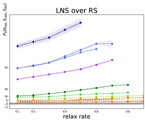
(a) Diversity improvement

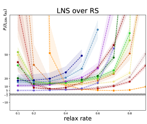
(b) Diversification time overhead

Figure 6: Improvement in diversity and diversification time overhead of LNS over RS for different values of the relax rate

Appendix B Diversification Example

This section shows a more elaborated example of diversified code using DivCon. Figure 7 shows two variants of function ulaw2alaw from application g721. This function converts u-law ($\mu$-law) values to a-law ($A$-law) values. $\mu$-law and $A$-law are the two main companding algorithms of G.711 (?).

The two variants, Listing 7a and Listing 7b, are generated by DivCon with relax rate 0.6, optimality gap 10%, and the cycle hamming distance, $\delta_{HD}$. Figure 7 highlights four different ways in which the two variants differ. First, DivCon may add nop instructions. Interestingly, DivCon added an empty stack frame to Variant 2. The prologue (line 13 in Variant 2) and epilogue (line 42 in of Variant 2) instructions that build and destroy the empty stack frame are no-operations, however they contribute to the diversification of the function and their overhead does not exceed the optimality gap. Otherwise, DivCon adds MIPS nop instructions to fill the instruction schedule empty slots including the instruction delays due to their execution latency (see lines 19 and 20 of Variant 1). Another transformation is the addition of copy operations to move data from one register to the other (highlighted at line 16 of Variant 1). This transformation assists register renaming, which improves diversification. The third transformation that we have highlighted (lines 18-21 of Variant 1 and lines 17-18 of Variant 2) is instruction reordering. Here, whenever there is no data dependency between the instructions, the order of the instructions might change. Finally, the register assignment of different operations differs, with an example highlighted at line 26 of Variant 1 and line 25 of Variant 2. Other transformations, like spilling to the stack, are also possible. The function of Figure 7 is small and does not require spilling. However, DivCon may enable spilling if the overhead is not more than the allowed optimality gap (10% here).

Figure 7 shows also some of the gadgets that are available in function ulaw2alaw. In particular, both variants contain a number of gadgets that all include the last gadget, consisting of a return jump, jr, and its delay slot (following the branch). No pair of gadgets in the two variants is identical with regards to the content or the position in the code.

⬇

13ulaw2alaw: # @ulaw2alaw

14 .frame $sp,0,$ra

15 .mask 0x00000000,0

16 .fmask 0x00000000,0

17 .set noreorder

18 .set nomacro

19 .set noat

20# BB#0:

21 lui $v0, _gp_disp

22 nop

23 addiu $v0, $v0, _gp_disp

24 andi $a2, $a0, 128

25 beqz $a2, $BB0_2

26 addu $t7, $v0, $t9

27# BB#1:

28 move $t9, $a0

29 move $fp, $t9

30 lw $t2, _u2a($t7)

31 nop

32 nop

33 xori $t5, $fp, 255

34 addu $t8, $t2, $t5

35 lbu $a1, 0($t8)

36 nop

37 nop

38 addiu $t8 , $a1, -1

39 b $BB0_3

40 xori $a0, $t8, 213

41$BB0_2:

42 lw $v0, _u2a($t7)

43 nop

44 nop

45 xori $a1, $a0, 127

46 addu $t0, $v0, $a1

47 lbu $t3, 0($t0)

48 nop

49 nop

50 move $t6, $t3

51 move $a0, $t6

52 addiu $fp, $a0, -1

53 xori $a0, $fp, 85

54$BB0_3:

55 jr $ra

56 andi $v0, $a0, 255

(a) g721.g711.ulaw2alaw - Variant 1

⬇

13ulaw2alaw: # @ulaw2alaw

14 .frame $sp,0,$ra

15 .mask 0x00000000,0

16 .fmask 0x00000000,0

17 .set noreorder

18 .set nomacro

19 .set noat

20# BB#0:

21 lui $v0, _gp_disp

22 nop

23 addiu $v0, $v0, _gp_disp

24 andi $fp, $a0, 128

25 addiu $sp, $sp, 0

26 beqz $fp, $BB0_2

27 addu $a1, $v0, $t9

28# BB#1:

29 xori $t5, $a0, 255

30 lw $t6, _u2a($a1)

31 nop

32 nop

33 addu $v0, $t6, $t5

34 lbu $t1, 0($v0)

35 nop

36 nop

37 addiu $t3 , $t1, -1

38 b $BB0_3

39 xori $fp, $t3, 213

40$BB0_2:

41 xori $a3, $a0, 127

42 lw $t4, _u2a($a1)

43 nop

44 nop

45 addu $gp, $t4, $a3

46 lbu $t2, 0($gp)

47 nop

48 nop

49 addiu $t6, $t2, -1

50 xori $fp, $t6, 85

51$BB0_3:

52 andi $v0, $fp, 255

53 jr $ra

54 addiu $sp, $sp, 0

55 .set at

56 .set macro

(b) g721.g711.ulaw2alaw - Variant 2

Figure 7: Example function diversification in MIPS32 assembly code

References

- Abrath, B., Coppens, B., Mishra, M., den Broeck, J. V., and Sutter, B. D. (2020). Breakpad: Diversified binary crash reporting. IEEE Transactions on Dependable Secure Computing, 17(4), 841–856.
- Alaba, F. A., Othman, M., Hashem, I. A. T., and Alotaibi, F. (2017). Internet of Things security: A survey. Journal of Network and Computer Applications, 88, 10–28.
- Arteaga, J. C., Malivitsis, O. F., Pérez, O. L. V., Baudry, B., and Monperrus, M. (2021). Crow: Code diversification for webassembly. In MADWeb’21-NDSS Workshop on Measurements, Attacks, and Defenses for the Web.
- Ashouri, A. H., Killian, W., Cavazos, J., Palermo, G., and Silvano, C. (2018). A survey on compiler autotuning using machine learning. ACM Computing Surveys (CSUR), 51(5), 1–42.
- Baudry, B., Allier, S., and Monperrus, M. (2014). Tailored source code transformations to synthesize computationally diverse program variants. In Proc. of ISSTA, pp. 149–159.
- Baudry, B., and Monperrus, M. (2015). The Multiple Facets of Software Diversity: Recent Developments in Year 2000 and Beyond. ACM Comput. Surv., 48(1), 16:1–16:26.
- Birman, K. P., and Schneider, F. B. (2009). The monoculture risk put into context. IEEE Security & Privacy, 7(1), 14–17.
- Bletsch, T., Jiang, X., Freeh, V. W., and Liang, Z. (2011). Jump-oriented Programming: A New Class of Code-reuse Attack. In Proceedings of the 6th ACM Symposium on Information, Computer and Communications Security, ASIACCS ’11, pp. 30–40, New York, NY, USA. ACM.
- Braden, K., Crane, S., Davi, L., Franz, M., Larsen, P., Liebchen, C., and Sadeghi, A.-R. (2016). Leakage-Resilient Layout Randomization for Mobile Devices. In Proceedings 2016 Network and Distributed System Security Symposium, San Diego, CA. Internet Society.
- Castañeda Lozano, R., Carlsson, M., Blindell, G. H., and Schulte, C. (2019). Combinatorial Register Allocation and Instruction Scheduling. ACM Trans. Program. Lang. Syst., 41(3), 17:1–17:53.
- Castañeda Lozano, R., Carlsson, M., Drejhammar, F., and Schulte, C. (2012). Constraint-Based Register Allocation and Instruction Scheduling. In Milano, M. (Ed.), Principles and Practice of Constraint Programming, Lecture Notes in Computer Science, pp. 750–766, Berlin, Heidelberg. Springer.
- Checkoway, S., Davi, L., Dmitrienko, A., Sadeghi, A.-R., Shacham, H., and Winandy, M. (2010). Return-oriented Programming Without Returns. In Proceedings of the 17th ACM Conference on Computer and Communications Security, CCS ’10, pp. 559–572, New York, NY, USA. ACM.
- Chen, Y., Wang, Z., Whalley, D., and Lu, L. (2016). Remix: On-demand Live Randomization. In Proceedings of the Sixth ACM Conference on Data and Application Security and Privacy, CODASPY ’16, pp. 50–61, New York, NY, USA. Association for Computing Machinery.
- Chu, G. G. (2011). Improving combinatorial optimization. Ph.D. thesis, The University of Melbourne, Australia.
- Cohen, F. B. (1993). Operating system protection through program evolution.. Comput. Secur., 12(6), 565–584.
- Crane, S., Liebchen, C., Homescu, A., Davi, L., Larsen, P., Sadeghi, A., Brunthaler, S., and Franz, M. (2015). Readactor: Practical Code Randomization Resilient to Memory Disclosure. In 2015 IEEE Symposium on Security and Privacy, pp. 763–780.
- Davi, L. V., Dmitrienko, A., Nürnberger, S., and Sadeghi, A.-R. (2013). Gadge me if you can: secure and efficient ad-hoc instruction-level randomization for x86 and ARM. In Proceedings of the 8th ACM SIGSAC symposium on Information, computer and communications security, pp. 299–310. tex.organization: ACM.
- Forrest, S., Somayaji, A., and Ackley, D. H. (1997). Building diverse computer systems. In Proceedings. The Sixth Workshop on Hot Topics in Operating Systems (Cat. No. 97TB100133), pp. 67–72. IEEE.
- Gecode Team (2020). Gecode: Generic constraint development environment. Online: https://www.gecode.org.
- Hamming, R. W. (1950). Error detecting and error correcting codes. The Bell system technical journal, 29(2), 147–160.
- Hebrard, E., Hnich, B., O’Sullivan, B., and Walsh, T. (2005). Finding Diverse and Similar Solutions in Constraint Programming. In National Conference on Artificial Intelligence and the Seventeenth Innovative Applications of Artificial Intelligence Conference, p. 6.
- Homescu, A., Jackson, T., Crane, S., Brunthaler, S., Larsen, P., and Franz, M. (2017). Large-Scale Automated Software Diversity—Program Evolution Redux. IEEE Transactions on Dependable and Secure Computing, 14(2), 158–171.
- Homescu, A., Neisius, S., Larsen, P., Brunthaler, S., and Franz, M. (2013). Profile-guided Automated Software Diversity. In Proceedings of the 2013 IEEE/ACM International Symposium on Code Generation and Optimization (CGO), CGO ’13, pp. 1–11, Washington, DC, USA. IEEE Computer Society.
- Ingmar, L., de la Banda, M. G., Stuckey, P. J., and Tack, G. (2020). Modelling diversity of solutions. In Proceedings of the thirty-fourth AAAI conference on artificial intelligence.
- ITU, T. (1993). General aspects of digital transmission systems. ITU-T Recommendation G, 729.
- Jacob, M., Jakubowski, M. H., Naldurg, P., Saw, C. W. N., and Venkatesan, R. (2008). The Superdiversifier: Peephole Individualization for Software Protection. In Matsuura, K., and Fujisaki, E. (Eds.), Advances in Information and Computer Security, Lecture Notes in Computer Science, pp. 100–120, Berlin, Heidelberg. Springer.
- Kc, G. S., Keromytis, A. D., and Prevelakis, V. (2003). Countering code-injection attacks with instruction-set randomization. In Proc. of CCS, pp. 272–280.
- Koo, H., Chen, Y., Lu, L., Kemerlis, V. P., and Polychronakis, M. (2018). Compiler-Assisted Code Randomization. In 2018 IEEE Symposium on Security and Privacy (SP), pp. 461–477.
- Kornau, T., et al. (2010). Return oriented programming for the ARM architecture. Master’s thesis, Ruhr-Universität Bochum.
- Krueger, C. W. (1992). Software reuse. ACM Comput. Surv., 24(2), 131–183.
- Larsen, P., Homescu, A., Brunthaler, S., and Franz, M. (2014). SoK: Automated Software Diversity. In 2014 IEEE Symposium on Security and Privacy, pp. 276–291.
- Lattner, C., and Adve, V. (2004). LLVM: A compilation framework for lifelong program analysis & transformation. In Code Generation and Optimization. IEEE.
- Lee, C., Potkonjak, M., and Mangione-Smith, W. H. (1997). MediaBench: A tool for evaluating and synthesizing multimedia and communicatons systems. In International Symposium on Microarchitecture, pp. 330–335. IEEE.
- Lee, S., Kang, H., Jang, J., and Kang, B. B. (2021). Savior: Thwarting stack-based memory safety violations by randomizing stack layout..
- Lundquist, G. R., Bhatt, U., and Hamlen, K. W. (2019). Relational processing for fun and diversity. In Proceedings of the 2019 miniKanren and relational programming workshop, p. 100.
- Lundquist, G. R., Mohan, V., and Hamlen, K. W. (2016). Searching for Software Diversity: Attaining Artificial Diversity Through Program Synthesis. In Proceedings of the 2016 New Security Paradigms Workshop, NSPW ’16, pp. 80–91, New York, NY, USA. ACM.
- Pappas, V., Polychronakis, M., and Keromytis, A. D. (2012). Smashing the Gadgets: Hindering Return-Oriented Programming Using In-place Code Randomization. In 2012 IEEE Symposium on Security and Privacy, pp. 601–615.
- Petit, T., and Trapp, A. C. (2015). Finding Diverse Solutions of High Quality to Constraint Optimization Problems. In Twenty-Fourth International Joint Conference on Artificial Intelligence.
- Salehi, M., Hughes, D., and Crispo, B. (2019). Microguard: Securing bare-metal microcontrollers against code-reuse attacks. In 2019 IEEE Conference on Dependable and Secure Computing (DSC), pp. 1–8. IEEE.
- Salwan, J. (2020). ROPgadget Tool. Online: http://shell-storm.org/project/ROPgadget/.
- Shacham, H. (2007). The Geometry of Innocent Flesh on the Bone: Return-into-libc Without Function Calls (on the x86). In Proceedings of the 14th ACM Conference on Computer and Communications Security, CCS ’07, pp. 552–561, New York, NY, USA. ACM.
- Shaw, P. (1998). Using Constraint Programming and Local Search Methods to Solve Vehicle Routing Problems. In Maher, M., and Puget, J.-F. (Eds.), Principles and Practice of Constraint Programming — CP98, Lecture Notes in Computer Science, pp. 417–431, Berlin, Heidelberg. Springer.
- Snow, K. Z., Monrose, F., Davi, L., Dmitrienko, A., Liebchen, C., and Sadeghi, A. (2013). Just-In-Time Code Reuse: On the Effectiveness of Fine-Grained Address Space Layout Randomization. In 2013 IEEE Symposium on Security and Privacy, pp. 574–588.
- Sweetman, D. (2006). See MIPS Run, Second Edition. Morgan Kaufmann.
- Tsoupidi, R. M., Castañeda Lozano, R., and Baudry, B. (2020). Constraint-based software diversification for efficient mitigation of code-reuse attacks. In International Conference on Principles and Practice of Constraint Programming, pp. 791–808. Springer.
- Van Hentenryck, P., Coffrin, C., and Gutkovich, B. (2009). Constraint-Based Local Search for the Automatic Generation of Architectural Tests. In Gent, I. P. (Ed.), Principles and Practice of Constraint Programming - CP 2009, Lecture Notes in Computer Science, pp. 787–801. Springer Berlin Heidelberg.
- Wagner, R. A., and Fischer, M. J. (1974). The string-to-string correction problem. Journal of the ACM (JACM), 21(1), 168–173.
- Wang, S., Wang, P., and Wu, D. (2017). Composite Software Diversification. In 2017 IEEE International Conference on Software Maintenance and Evolution (ICSME), pp. 284–294.
- Wartell, R., Mohan, V., Hamlen, K. W., and Lin, Z. (2012). Binary Stirring: Self-randomizing Instruction Addresses of Legacy x86 Binary Code. In Proceedings of the 2012 ACM Conference on Computer and Communications Security, CCS ’12, pp. 157–168, New York, NY, USA. ACM.
- Williams-King, D., Gobieski, G., Williams-King, K., Blake, J. P., Yuan, X., Colp, P., Zheng, M., Kemerlis, V. P., Yang, J., and Aiello, W. (2016). Shuffler: Fast and Deployable Continuous Code Re-Randomization.. pp. 367–382.