An Abstract Model for Branch and Cut

Abstract

Branch and cut is the dominant paradigm for solving a wide range of mathematical programming problems — linear or nonlinear — combining efficient search (via branch and bound) and relaxation-tightening procedures (via cutting planes, or cuts). While there is a wealth of computational experience behind existing cutting strategies, there is simultaneously a relative lack of theoretical explanations for these choices, and for the tradeoffs involved therein. Recent papers have explored abstract models for branching and for comparing cuts with branch and bound. However, to model practice, it is crucial to understand the impact of jointly considering branching and cutting decisions. In this paper, we provide a framework for analyzing how cuts affect the size of branch-and-cut trees, as well as their impact on solution time. Our abstract model captures some of the key characteristics of real-world phenomena in branch-and-cut experiments, regarding whether to generate cuts only at the root or throughout the tree, how many rounds of cuts to add before starting to branch, and why cuts seem to exhibit nonmonotonic effects on the solution process.

1 Introduction

The branch-and-cut (B&C) paradigm is a hybrid of the branch-and-bound (B&B) [28] and cutting plane methods [18, 19, 20]. It is central to a wide range of modern global optimization approaches [10, 4], particularly mixed-integer linear and nonlinear programming solvers [23]. Cutting planes, or cuts, tighten the relaxation of a given optimization problem and are experimentally known to significantly improve a B&B process [3], but determining which cuts to add is currently based on highly-engineered criteria and computational insights, not from theory. An outstanding open problem is a rigorous underpinning for the choices involved in branch and cut. While recent papers have been actively exploring the theory of branching [29, 5, 12, 14, 13] and comparing cutting and branching [8], the interaction of the two together remains poorly understood. Most recently, Basu, Conforti, Di Summa, and Jiang [7] have proved that using B&C can strictly outperform either branching or cutting alone.

This paper introduces a theoretical framework for analyzing the practical challenges involved in making B&C decisions. We build on work by Le Bodic and Nemhauser [29], which provides an abstract model of B&B, based on how much bound improvement is gained by branching on a variable at a node of the B&B tree. This model not only is theoretically useful, but also can improve branching decisions in solvers [5].

Specifically, we add a cuts component to the abstract B&B model from Le Bodic and Nemhauser [29]. We apply this enhanced model to account for both the utility of the cuts in proving bounds, as well as the additional time taken to solve the nodes of a B&C tree after adding cuts.

In this abstract model, given the relative strengths of cuts, branching, and the rate at which node-processing time grows with additional cuts, we quantify (i) the number of cuts, and (ii) cut positioning (at the root or deeper in the tree) to minimize both the tree size and the solution time of an instance. This thereby captures some of the main tradeoffs between cutting and branching, in that cuts can improve the bound or even the size of a B&C tree, but meanwhile slow down the solution time overall. We use a single-variable abstract B&C model, where every branching variable has identical effect on the bound, and we only address the dual side of the problem, i.e., we are only interested in proving a good bound on the optimal value, as opposed to generating better integer-feasible solutions.

We emphasize that our motivation is to advance a theoretical understanding of empirically-observed phenomena in solving optimization problems, and our results show that some of the same challenges that solvers encounter in applying cuts do arise in theory. While we state prescriptive recommendations in our abstract model, these are not intended to be immediately computationally viable. Instead, the intent of the prescriptive results is to see whether our abstraction affords enough simplicity to make precise theoretical statements.

Summary of contributions and paper structure.

We provide a generic view of B&C in Section 2. Section 3 introduces our abstract B&C model, in which the quality of cuts and branching remains fixed throughout the tree. In Section 4, we analyze the effect of cuts on tree size; we prove that in this case it is never necessary to add cuts after the root node, and we provide a lower bound on the optimal number of cutting plane rounds that will minimize the B&C tree size. In Section 5, we extend our model to account for diminishing marginal returns from cuts, relaxing our assumption of constant cut strength. Our main result in this section is an approximation of the optimal number of cuts.

Then, in Section 6, we study how cuts affect solving time for a tree, not just its size, under constant cut strength. In Section 6.1, we show that cuts are guaranteed to be helpful for sufficiently hard instances. In contrast to the case of tree size, in this more general setting, adding cuts after the root node may be better. However, in Theorem 23, we show that when the two branching directions yield the same bound improvement, then root cuts are still sufficient.

2 Preliminaries

We are given a generic optimization problem (OP) — linear or nonlinear, with or without integers — which is to be solved using a B&C algorithm. For convenience, we assume that the OP is a minimization problem. We also assume that we already have a feasible solution to the OP, so that our only goal is to efficiently certify the optimality or quality of that solution.

The B&C approach involves creating a computationally tractable relaxation of the original problem, which we call the root of the B&C tree and assume is provided to us. For example, when the OP is a mixed-integer linear program, we start with its linear programming relaxation. The value of the solution to this relaxation provides a lower bound on the optimal value to the OP. B&C proceeds by either (1) tightening the relaxation through adding valid cuts, which will remove parts of the current relaxation but no OP-feasible points, or (2) splitting the feasible region, creating two subproblems, which we call the children of the original (parent) relaxation. Both of these operations improve the lower bound with respect to the original relaxation. The B&C procedure repeats on the new relaxation with cuts added in the case of (1), and recursively on the children in the case of (2); we assume that tractability is maintained in either case. Moreover, we assume that all children remain OP-feasible. We now formally define a B&C tree as used in this paper.

Definition 1 (B&C tree).

A B&C tree $T$ is a rooted binary tree with node set $\mathcal{V}_{T}$ that is node-labeled by a function $z_{\scriptscriptstyle T}:\mathcal{V}_{T}\to\mathbb{R}_{\scriptscriptstyle\geq 0}$, indicating the bound improvement at each node with respect to the bound at the root node, such that

1. The root node $v_{0}$ has label $z_{\scriptscriptstyle T}(v_{0})=0$.

2. A node $v$ with exactly one child $v^{\prime}$ is a cut node, and we say that a cut or round of cuts is added at node $v$. The bound at $v^{\prime}$ is $z_{\scriptscriptstyle T}(v^{\prime})=z_{\scriptscriptstyle T}(v)+c_{v}$, where $c_{v}$ is the nonnegative value associated with the round of cuts at $v$.

3. A node $v$ with exactly two children $v_{1}$ and $v_{2}$ is a branch node, and we say that we branch at node $v$. The bounds at the children of $v$ are $z_{\scriptscriptstyle T}(v_{1})=z_{\scriptscriptstyle T}(v)+\ell_{v}$ and $z_{\scriptscriptstyle T}(v_{2})=z_{\scriptscriptstyle T}(v)+r_{v}$, where $(\ell_{v},r_{v})$ is the pair of bound improvement values associated with branching at $v$.

4. A node with no children is a leaf node.

We say that $T$ proves a bound of $Z$ if $z_{\scriptscriptstyle T}(v)\geq Z$ for all leaves $v\in\mathcal{V}_{T}$.

We will refer to a cut-and-branch tree as one in which all cut nodes are at the root, before the first branch node.

While Definition 1 is generic, the abstraction we study is restricted to the single-variable version in which $\ell_{v}$ and $r_{v}$ are the same for each branch node $v\in\mathcal{V}_{T}$. We also drop the subscript $v$ in $c_{v}$, as in Section 4 and Section 6, we assume a constant cut quality for each cut node $v\in\mathcal{V}_{T}$, while in Section 5, cut quality is only a function of the number of cuts already applied.

3 The Abstract Branch-and-Cut Model

This section introduces the Single Variable Branch-and-Cut (SVBC) model, an abstraction of a B&C tree as presented in Definition 1. First, we define a formal notion of the time taken to process a B&C tree as the sum of the node processing times, which in turn depends on the following definition of a time-function.

Definition 2 (Time-function).

A function $\operatorname{w}:\mathbb{Z}_{\scriptscriptstyle\geq 0}\to[1,\infty)$ is a time-function if it is nondecreasing and $\operatorname{w}(0)=1$.

Definition 3 (Node time and tree time).

Given a B&C tree $T$, node $v\in\mathcal{V}_{T}$, and time-function $\operatorname{w}$,

1. the (node) time of $v$, representing the time taken to process node $v$, is $\operatorname{w}(z)$, where $z$ is the number of cut nodes in the path from the root of $T$ to $v$.

2. the (tree) time of $T$, denoted by $\operatorname{\tau}_{\operatorname{w}}(T)$, is the sum of the node times of all the nodes in the tree.

We simply say $\operatorname{\tau}(T)$ when the time-function $\operatorname{w}$ is clear from context.

Definition 3 models the observation that cuts generally make the relaxation harder to solve, and hence applying more cuts increases node processing time. Note that (i) if $\operatorname{w}=\mathbf{1}$, i.e., $\operatorname{w}(z)=1$ for all $z\in\mathbb{Z}_{\scriptscriptstyle\geq 0}$, we obtain the regular notion of size of a tree, which counts the number of nodes in the tree, and (ii) the time of a pure cutting tree with $t$ cuts (i.e., $t+1$ nodes) is $\sum_{i=0}^{t}\operatorname{w}(i)$.

Finally, we state the SVBC model in Definition 4. In this model, the relative bound improvement at every cut node is always the same constant $c$, and every branch node is associated to the same $(\ell,r)$ pair of bound improvement values. We also assume that the time to solve a node depends on the number of cuts added to the relaxation up to that node.

Definition 4 (Single Variable Branch-and-Cut (SVBC) Tree).

A B&C tree is a Single Variable Branch-and-Cut (SVBC) tree with parameters $(\ell,r;c,\operatorname{w})$ if the bound improvement value associated with each branch node is $(\ell,r)$, the bound improvement by each cut node is $c$, and the time-function is $\operatorname{w}$. We say such a tree is an $\mathop{SV\!BC}(\ell,r;c,\operatorname{w})$ tree.

Without loss of generality, we assume $0\leq\ell\leq r$.

Definition 5 ($\operatorname{\tau}$-minimality).

Given a function $\operatorname{w}:\mathbb{Z}_{\scriptscriptstyle\geq 0}\to[1,\infty)$, we say that a B&C tree $T$ that proves bound $Z$ is $\operatorname{\tau}$-minimal if, for any other B&C tree $T^{\prime}$ that also proves bound $Z$ with the same $(\ell,r;c,\operatorname{w})$, it holds that $\operatorname{\tau}(T^{\prime})\geq\operatorname{\tau}(T)$.

When $\operatorname{w}=\mathbf{1}$, we may refer to a $\operatorname{\tau}$-minimal tree as minimal-sized.

It is often the case that applying a round of cuts at a node may not improve the bound as much as branching at that node, but the advantage is that cutting adds only one node to the tree, while branching creates two subproblems. A first question is whether there always exists a minimal-size tree with only branch nodes or only cut nodes. We address this in Example 6, which illustrates our notation, shows that cut nodes can help reduce the size of a B&C tree despite improving the bound less than branch nodes, and highlights the fact that finding a minimal-sized B&C tree proving a particular bound $Z$ involves strategically using both branching and cutting.

Example 6 (Branch and cut can outperform pure branching or pure cutting).

for tree = big node [0 [3 [6] [6] ] [3 [6] [6] ] ]

(a) Pure branching: 7 nodes

for tree = big node [0,big cut [1,big cut [,dot node [5,big cut [6]]]]]

(b) Pure cutting: 7 nodes

for tree = big node [0,big cut [1,big cut [2,big cut [3 [6] [6] ] ] ] ]

(c) Branch and cut: 6 nodes

Figure 1: Three B&C trees proving $Z=6$, with $\ell=r=3$, $c=1$, and $\operatorname{w}=\mathbf{1}$.

Figure 1 shows three B&C trees that prove the bound $Z=6$. The tree in panel 1(a) only has branch nodes, 1(b) only has cut nodes, and 1(c) has both branch and cut nodes. As seen in the figure, branching and cutting together can create strictly smaller trees than pure branching or cutting methods. $\blacksquare$

Basu, Conforti, Di Summa, and Jiang [8, 7] also investigate the complementary effect of branching and cutting. The authors prove that for pure binary problems, when cutting and branching are derived from the same underlying logical conditions, then it suffices to only cut to minimize the size of the tree [8]. When the second assumption is relaxed, the second paper proves that combining cutting and branching can be exponentially better than using either method alone [7]. We instead focus on specifying the optimal number of cuts to add or where to place them in the tree for a particular instance.

4 Optimizing Tree Size

In this section, we examine the number of cuts that minimize the size $\lvert\mathcal{V}_{T}\rvert$ of a B&C tree $T$, i.e., optimizing $\operatorname{\tau}(T)$ when $\operatorname{w}=\mathbf{1}$. In Lemma 7, we first address the location of these cuts — should they be at the root or deeper in the tree?

Lemma 7.

For any target bound $Z$ and a fixed set of parameters $(\ell,r;c,\mathbf{1})$, there exists a $\operatorname{\tau}$-minimal $\mathop{SV\!BC}(\ell,r;c,\mathbf{1})$ tree that proves bound $Z$ such that all cut nodes form a path starting at the root of the tree.

Proof.

Let $T$ be a $\operatorname{\tau}$-minimal $\mathop{SV\!BC}(\ell,r;c,\mathbf{1})$ tree. If all cut nodes in the tree $T$ are at the root, then we are done. Otherwise, let $v\in\mathcal{V}_{T}$ be a cut node with a parent that is a branch node, i.e., $v$ has one child $w$. Let $T^{\prime}$ be the tree obtained by removing $w$ from $T$, i.e., contracting $v$ and $w$, and instead inserting $w$ immediately after the root. Let $v^{\prime}\neq w$ be a leaf node of $T$, which is also a leaf of $T^{\prime}$. It holds that $z_{\scriptscriptstyle T^{\prime}}(v^{\prime})\geq z_{\scriptscriptstyle T}(v^{\prime})$, since the path from the root to $v^{\prime}$ in $T^{\prime}$ goes through the same branch nodes and at least as many cut nodes as in $T$. Recursively applying this procedure, we move all cut nodes to the root without increasing the tree size, proving the desired result by the assumed minimality of $T$. ∎

We have proved that for any minimal-size $\mathop{SV\!BC}(\ell,r;c,\mathbf{1})$ tree, it suffices to consider cut-and-branch trees, where all cut nodes are at the root. To understand how many cuts should be added, we start with the special case that $c\leq\ell=r$.

A useful observation for our analysis is that one should not evaluate the effects of cuts one at a time on the size of the tree, as tree size does not monotonically decrease as the number of cuts increases from $0$ to the optimal number of cuts. For example, if $c<\ell=r$ and $Z=2c\pmod{r}$, using one cut node would increase the overall tree size, while two cut rounds would reduce tree size by $2^{\left\lceil Z/r\right\rceil}-2$. This phenomenon highlights a practical challenge in determining how to use a cut family and whether cuts benefit an instance, as adding too few or too many cut nodes may increase tree size while the right number can greatly decrease the overall size.

Instead, the key insight for Theorem 9 is reasoning about layers: adding a set of cut nodes is beneficial when, together, the cut nodes improve the bound enough to remove an additional layer of the branch-and-bound tree, and fewer cuts are added than the number of removed nodes.

If a minimal-size tree $T$ proving bound $Z$ has $k$ cut nodes at the root, then the depth of the branching component, the subtree starting with the first branch node, is $0pt_{k}\mathrel{\vbox{\hbox{\footnotesize.}\hbox{\footnotesize.}}}=\max\{0,\left\lceil(Z-ck)/r\right\rceil\}$. The total size of the tree is $\operatorname{\tau}(T)=k+2^{0pt_{k}+1}-1$. We also know that the depth of the branching component when the target bound is $Z$ is never more than $0pt^{\max}\mathrel{\vbox{\hbox{\footnotesize.}\hbox{\footnotesize.}}}=\left\lceil Z/r\right\rceil.$

For any given $0pt\in\{0,\ldots,0pt^{\max}\}$ and target bound $Z$, the minimum number of cut nodes at the root to achieve that depth of the branching component is

$$\kappa_{\scriptscriptstyle Z}(0pt)\mathrel{\vbox{\hbox{\footnotesize.}\hbox{\footnotesize.}}}=\max\{0,\left\lceil(Z-0ptr)/c\right\rceil\},$$

where it can be seen that $\kappa_{\scriptscriptstyle Z}(0pt)=0$ if and only if $0pt=0pt^{\max}$, within the domain.

Lemma 8.

When $0<c\leq\ell=r$, the optimal number of cut nodes in a minimal-size SVBC tree proving bound $Z$ is $\kappa_{\scriptscriptstyle Z}(0pt)$ for some $0pt\in\mathbb{Z}_{\scriptscriptstyle\geq 0}$.

Proof.

A branching component with depth $0pt$ proves a bound $0ptr$, leaving a bound of $\max\{0,Z-0ptr\}$ to prove with cut nodes. Therefore, it is necessary and sufficient to use $\kappa_{\scriptscriptstyle Z}(0pt)=\max\left\{0,\left\lceil{(Z-0ptr)}/{c}\right\rceil\right\}$ cut nodes. ∎

Next, we present Theorem 9, which provides the optimal number of rounds of cuts for an $\mathop{SV\!BC}(\ell,r;c,\mathbf{1})$ tree when $c\leq\ell=r$, as a function of the tree parameters and the target bound. The theorem implies that the depth of the branching component in a minimal-size tree can take one of four values, and it is at most $0pt^{*}\mathrel{\vbox{\hbox{\footnotesize.}\hbox{\footnotesize.}}}=\left\lfloor\log_{2}\left\lceil{r}/{c}\right\rceil\right\rfloor$, which is independent of the target bound $Z$. Thus, as $Z$ increases, the proportion of the bound proved by branch nodes goes to zero.

Theorem 9.

Let $0pt^{*}\mathrel{\vbox{\hbox{\footnotesize.}\hbox{\footnotesize.}}}=\left\lfloor\log_{2}\left\lceil{r}/{c}\right\rceil\right\rfloor$. When $0<c\leq\ell=r$, the number of cut nodes to minimize the size of an $\mathop{SV\!BC}(\ell,r;c,\mathbf{1})$ tree proving bound $Z$ is

$$k^{*}\mathrel{\vbox{\hbox{\footnotesize.}\hbox{\footnotesize.}}}=\begin{cases}\kappa_{\scriptscriptstyle Z}(0pt^{*})&\text{if $Z\geq r0pt^{*}$ and $\kappa_{\scriptscriptstyle Z}(0pt^{*}-1)-\kappa_{\scriptscriptstyle Z}(0pt^{*})\geq 2^{0pt^{*}}$}\\ \kappa_{\scriptscriptstyle Z}(0pt^{*}-1)&\text{if $Z\geq r0pt^{*}$ and $\kappa_{\scriptscriptstyle Z}(0pt^{*}-1)-\kappa_{\scriptscriptstyle Z}(0pt^{*})<2^{0pt^{*}}$}\\ \kappa_{\scriptscriptstyle Z}(0pt^{\max}-1)&\text{if $Z<r0pt^{*}$ and $\kappa_{\scriptscriptstyle Z}(0pt^{\max}-1)<2^{0pt^{\max}}$}\\ 0&\text{otherwise.}\end{cases}$$

The optimal depth of the branching component is either $\min\{0pt^{*},0pt^{\max}\}$ or $\min\{0pt^{*},0pt^{\max}\}-1$. Moreover, the size of any minimal $\mathop{SV\!BC}(\ell,r;c,\mathbf{1})$ tree that proves bound $Z$ is at least $2^{\left\lceil(Z-ck^{*})/r\right\rceil+1}-1+k^{*}.$

Proof.

Given an instance for which bound $Z$ needs to be proved, our goal is to understand how the size of the $\text{SVBC}{(\ell,r;c,\mathbf{1})}$ tree changes as a function of $k$, the number of cuts we apply at the root node. By Lemma 8, our goal is equivalent to finding the optimal depth of the branching component.

Let $T_{0pt}$ denote the tree with $\kappa_{\scriptscriptstyle Z}(0pt)$ cuts added at the root node, followed by a branching component of depth $0pt$. Recall that $\kappa_{\scriptscriptstyle Z}(0pt)$ is the minimum number of cuts to achieve a branching depth of $0pt$. The bound $z_{\scriptscriptstyle T_{0pt}}(u)$ at each leaf node $u$ of $T_{0pt}$ satisfies $z_{\scriptscriptstyle T_{0pt}}(u)\geq Z$. Hence, for any node $v$ that is a parent of a leaf node $u$ of $T_{0pt}$, the bound at $v$ is $z_{\scriptscriptstyle T_{0pt}}(v)=z_{\scriptscriptstyle T_{0pt}}(u)-r\geq Z-r$. By definition of $\kappa_{\scriptscriptstyle Z}(0pt-1)$, $z_{\scriptscriptstyle T_{0pt}}(v)+(\kappa_{\scriptscriptstyle Z}(0pt-1)-\kappa_{\scriptscriptstyle Z}(0pt))c\geq Z$, as the last layer of the tree $T_{0}pt$ will no longer be necessary, and any fewer cuts will not meet the target bound:

$$z_{\scriptscriptstyle T_{0pt}}(v)+(\kappa_{\scriptscriptstyle Z}(0pt-1)-\kappa_{\scriptscriptstyle Z}(0pt)-1)c<Z.$$

Hence,

$$\kappa_{\scriptscriptstyle Z}(0pt-1)-\kappa_{\scriptscriptstyle Z}(0pt)<1+\frac{Z-z_{\scriptscriptstyle T_{0pt}}(v)}{c}\leq 1+\frac{r}{c},$$

so that the number of cuts to decrease the branching component by one more layer is at most $\kappa_{\scriptscriptstyle Z}(0pt-1)-\kappa_{\scriptscriptstyle Z}(0pt)\leq\left\lfloor r/c\right\rfloor$. As there are $2^{0}pt$ leaf nodes in the last layer of $T_{0}pt$, $\operatorname{\tau}(T_{0pt-1})>\operatorname{\tau}(T_{0pt})$ if and only if $\kappa_{\scriptscriptstyle Z}(0pt-1)-\kappa_{\scriptscriptstyle Z}(0pt)>2^{0pt}$, implying that adding the $\kappa_{\scriptscriptstyle Z}(0pt-1)-\kappa_{\scriptscriptstyle Z}(0pt)$ cut nodes is beneficial if $0pt>0pt^{*}=\left\lfloor\log_{2}\left\lceil{r}/{c}\right\rceil\right\rfloor$. This is independent of $Z$ and we conclude that, if $0pt^{*}\leq 0pt^{\max}$, then the optimal branching depth is at most $0pt^{*}$.

Now assume $0pt<0pt^{\max}$. For a leaf node $u$ of $T_{0pt}$, $z_{\scriptscriptstyle T_{0pt}}(u)<Z+c$, as the definition of $\kappa_{\scriptscriptstyle Z}(0pt)$ means $\kappa_{\scriptscriptstyle Z}(0pt)-1$ cut nodes would require another layer of branching to prove bound $Z$. For any node $v$ that is a parent of $u$, by definition of $\kappa_{\scriptscriptstyle Z}(0pt-1)$, $z_{\scriptscriptstyle T_{0pt}}(v)+(\kappa_{\scriptscriptstyle Z}(0pt-1)-\kappa_{\scriptscriptstyle Z}(0pt))c\geq Z,$ which, together with $z_{\scriptscriptstyle T_{0pt}}(v)<Z-r+c$, implies that, when $0pt<0pt^{\max}$, the number of cuts to decrease the branching component by one more layer is at least

$$\kappa_{\scriptscriptstyle Z}(0pt-1)-\kappa_{\scriptscriptstyle Z}(0pt)\geq\frac{Z-z_{\scriptscriptstyle T_{0pt}}(v)}{c}\geq\left\lceil\frac{r}{c}\right\rceil-1.$$ (1)

It follows that removing an additional layer weakly increases the size of the tree if $\left\lceil r/c\right\rceil-1\geq 2^{0pt}$, which holds if $0pt<0pt^{*}-1$, and so the optimal branching depth is at least $0pt^{*}-1$. Hence, the optimal number of cuts when $0pt^{*}\leq 0pt^{\max}$ is $\kappa_{\scriptscriptstyle Z}(0pt^{*})$ if $\kappa_{\scriptscriptstyle Z}(0pt^{*}-1)-\kappa_{\scriptscriptstyle Z}(0pt^{*})\geq 2^{0pt^{*}}$, and it is $\kappa_{\scriptscriptstyle Z}(0pt^{*}-1)$ otherwise.

The last case to consider is when $0pt^{*}>0pt^{\max}$, or equivalently $Z<r0pt^{*}$. For all $0pt\leq 0pt^{\max}\leq 0pt^{*}-1$, including the pure branch-and-bound tree, $T_{0pt}$ has at most $2^{0pt^{*}-1}\leq\left\lceil r/c\right\rceil-1$ leaf nodes. For depths $0pt<0pt^{\max}$, the lower bound in (1) implies that $\operatorname{\tau}(T_{0pt-1})\geq\operatorname{\tau}(T_{0pt})$. However, at $0pt=0pt^{\max}$, it is still possible that $\kappa_{\scriptscriptstyle Z}(0pt^{\max}-1)<2^{0pt^{\max}}$. This precisely results in the last two cases in the definition of $k^{*}$ in the theorem statement. ∎

In Theorem 10, we show that even in general, for $\ell\neq r$, it is always optimal to add at least one cut round for sufficiently large target bounds.

Theorem 10.

If $0<c\leq\ell\leq r$ and $Z>r\left\lfloor\log_{2}\left\lceil r/c\right\rceil\right\rfloor$, then the minimal $\mathop{SV\!BC}(\ell,r;c,\mathbf{1})$ tree proving a bound $Z$ has at least one cut node.

Proof.

Consider a pure branching tree that proves $Z$. The number of leaf nodes of this tree is at least $2^{\left\lceil Z/r\right\rceil}$, since $\ell\leq r$, and all the parents of each of these leaf nodes have a remaining bound in $(0,r]$ that needs to be proved. Now suppose we add $\left\lceil r/c\right\rceil$ rounds of cuts. All of the leaf nodes of the pure branch-and-bound tree would then be pruned, since the parent nodes would already prove the desired target bound of $Z$. As a result, there is benefit to cutting when $2^{\left\lceil Z/r\right\rceil}>\left\lceil r/c\right\rceil$, which holds when $Z>r\left\lfloor\log_{2}\left\lceil r/c\right\rceil\right\rfloor$. ∎

Corollary 11.

If $0<c\leq\ell\leq r$, then for $\overline{Z}\mathrel{\vbox{\hbox{\footnotesize.}\hbox{\footnotesize.}}}=r\left\lfloor\log_{2}\left\lceil r/c\right\rceil\right\rfloor$, every minimal $\mathop{SV\!BC}(\ell,r;c,\mathbf{1})$ tree proving a bound $Z>\overline{Z}$ has at least $\left\lceil\frac{Z-\overline{Z}}{c}\right\rceil$ cut nodes.

Example 12.

The following example, from Basu, Conforti, Di Summa, and Jiang [7], shows that SVBC trees with constant $c\leq\ell=r$ have been studied in the literature and that cuts not only decrease the size of a branch-and-bound tree, but in fact can lead to an exponential improvement.

Consider the independent set problem, defined on a graph $G$ with vertices $V$ and edge set $E$, in which $G$ consists of $m$ disjoint triangles (cliques of size three): $\max_{x}\{\sum_{v\in V}x_{v}:x\in\{0,1\}^{\lvert V\rvert};\;x_{u}+x_{v}\leq 1,\;\forall\,\{u,v\}\in E\}.$ The optimal value is $m$, using $x_{v}=1$ for exactly one vertex of every clique, while the linear relaxation has optimal value $3m/2$, obtained by setting $x_{v}=1/2$ for all $v\in V$.

Suppose we branch on $x_{v}$, $v\in V$, where $v$ belongs to a clique with vertices $u$ and $w$. In the left ($x_{v}\leq 0$) branch, the objective value of the relaxation decreases by $\ell=1/2$ with respect to the parent. This is because the optimal values of the variables for all vertices except $u$, $v$, and $w$ remain unchanged, and the constraint $x_{u}+x_{w}\leq 1$ along with $x_{v}\leq 0$ implies that the objective contribution of the triangle $\{u,v,w\}$ is at most $1$, whereas at the parent node $x_{u}+x_{v}+x_{w}$ contributed 3/2 to the objective. We can attain that contribution of $1$ by setting either $x_{u}=1$ and $x_{w}=0$, or $x_{w}=1$ and $x_{u}=0$. Similarly, for the right branch, we can derive that $r=1/2$.

Notice that once we branch on $x_{v}$, the remaining problem can be seen as fixing the values of the three variables corresponding to vertices in the triangle that $v$ belongs to, while keeping the remaining variables unchanged. In other words, it is a subproblem with exactly the same structure as the original one, except removing the decision variables for the vertices of a single clique.

Finally, we look at families of cutting planes that we can derive. By adding up the three constraints corresponding to the edges of any triangle $\{u,v,w\}$, we obtain the implication $2(x_{u}+x_{v}+x_{w})\leq 3$. Since all variables are integer-restricted, we can infer that $x_{u}+x_{v}+x_{w}\leq\left\lfloor 3/2\right\rfloor=1$ for every clique. Each such cut corresponds to a change of $c=1/2$ in the objective, and there exists one such cut for every clique of three vertices.

Hence, by Theorem 9, we have that, not counting cut nodes, the optimal depth of the $\mathop{SV\!BC}(\ell,r;c,\mathbf{1})$ tree that proves the bound $Z=m/2$ is $\delta^{*}=\left\lfloor\log_{2}\left\lceil r/c\right\rceil\right\rfloor=0$. This implies that the optimal number of cut rounds is

$$k^{*}=\left\lceil\frac{Z}{c}\right\rceil=\left\lceil\frac{m/2}{1/2}\right\rceil=m,$$

for a corresponding tree with $m$ total nodes, compared to a pure branching tree that would have depth $\left\lceil Z/r\right\rceil=m$ and thus $2^{m+1}-1$ nodes, which is exponentially many more than if cuts are used. $\blacksquare$

5 Diminishing Cut Strength

In the SVBC model, the assumption of constant cut strength $c$ implies that a tree with only cut nodes proving a bound $Z$ has size $1+\left\lceil Z/c\right\rceil$, growing linearly with $Z$. Meanwhile, the tree size to prove the same bound by only branch nodes is exponential in $Z$. While Example 12 illustrates that there exist cases where the constant cut strength assumption is satisfied, a more realistic setting would reflect the empirically-observed phenomenon of diminishing marginal bound improvements from cuts [6, 15]. In this section, we study tree size ($\operatorname{w}=\mathbf{1}$) when cuts deteriorate in strength across rounds, for the special case that $\ell=r$.

5.1 Empirical Motivation for Worsening Cuts

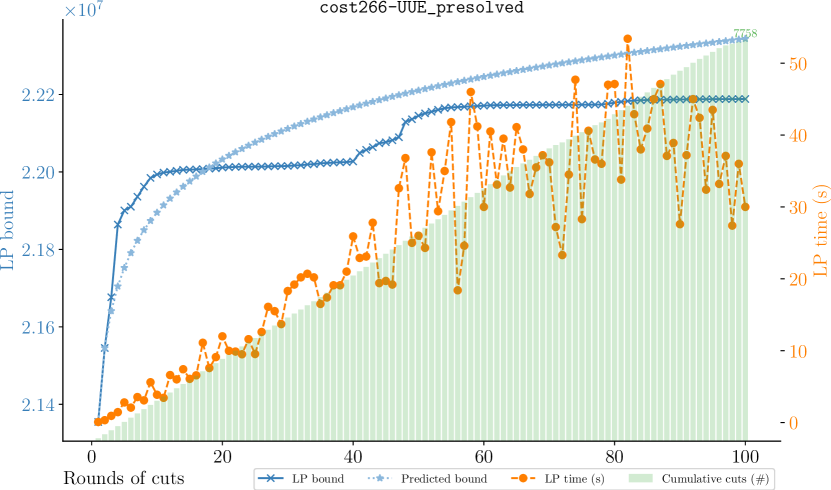
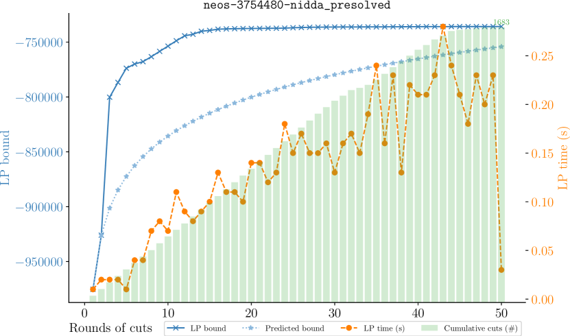
Figure 2: Applying rounds of Gomory cuts on two MIPLIB 2017 instances (after preprocessing) yields a diminishing bound improvement (LP bound) and a linear tendency for LP resolve time (LP time). The overlayed bar plot for each instance shows the cumulative number of cuts added after each round. The predicted bound using the improvement from the first round follows a logarithmic function that is similar to the actual bound evolution.

We first test 12 instances from the 2017 Mixed Integer Programming Library [17] as examples of the evolution of the bound as rounds of cuts are applied at the root node on an optimization solver. The subset of instances is based on auxiliary testing showing that they have linear relaxations that solve relatively quickly and that Gomory mixed-integer cuts [19] nontrivially affect the bound. We do not claim these instances are representative.

Specifically, we apply rounds of Gomory mixed-integer cuts to instances that are first presolved using Gurobi [21]. Cuts are computed in each round with the CglGMI implementation in the Cut Generation Library [1]. The linear relaxation after each round of cuts is solved using Clp [2]. Cut generation is terminated after either 100 rounds of cuts have been applied, one hour has elapsed, or no cuts are generated in a given round. Experiments are performed with a single thread on HiPerGator, a shared cluster through Research Computing at the University of Florida.

Figure 2 depicts the results for two instances. Each plot shows four time series after rounds of cuts: the linear relaxation optimal value (“LP bound”), the “Predicted bound” corresponding to the model in Section 5.2, the number of seconds it takes to solve the linear relaxation (“LP time”), and the total number of cuts in the relaxation (“Cumulative cuts”). The results for the remaining 10 instances are plotted in Figure 6 in Appendix A. For the predicted bound series, the bound in round $t$ is based on the first round of cuts: if $z_{0}$ is the initial linear programming relaxation optimal value, and $z_{1}$ is the value of the linear relaxation after one round of cuts, then the predicted bound $\widetilde{z}_{t}$ at round $t$ is computed as $\widetilde{z}_{t}\mathrel{\vbox{\hbox{\footnotesize.}\hbox{\footnotesize.}}}=\widetilde{z}_{t-1}+(z_{1}-z_{0})/t$, where $\widetilde{z}_{0}\mathrel{\vbox{\hbox{\footnotesize.}\hbox{\footnotesize.}}}=z_{0}$.

Across the instances, we observe that cuts tend to provide diminishing marginal bound improvements as more rounds are applied. Furthermore, the predicted bound follows a logarithmic function that reflects the general trend in the bound, though it becomes less accurate in later rounds when there is more substantial tailing off in bound improvement.

The model introduced next only aims to capture the relative decrease in how cuts affect the bound across rounds. The time to solve the linear relaxation as a function of number of cut rounds is further discussed in Section 6.

5.2 Single Variable Branching with Harmonically-Worsening Cuts

We define a model in which the total bound improvement by $k$ cuts is the $k$th harmonic number scaled by a constant parameter $c$, so that the number of cuts needed to prove a bound $Z$ grows exponentially in $Z$. Thus, we have two exponential-time procedures (pure cutting and pure branching) that can work together to prove the target bound. Let $H:\mathbb{Z}_{\scriptscriptstyle\geq 0}\to\mathbb{R}_{\scriptscriptstyle\geq 0}$ denote the $k$th harmonic number $H(k)\mathrel{\vbox{\hbox{\footnotesize.}\hbox{\footnotesize.}}}=\sum_{i=1}^{k}1/i$.

Definition 13 (Single Variable Branching with Harmonically-Worsening Cuts (SVBHC)).

A B&C tree is a Single Variable Branching with Harmonically-Worsening Cuts (SVBHC) tree with parameters $(\ell,r;c,\operatorname{w})$, or $\mathop{SV\!BH\!C}(\ell,r;c,\operatorname{w})$ tree, if the bound improvement value associated with each branch node is $(\ell,r)$, the bound improvement by cut node $k$ is $c/k$, and the time-function is $\operatorname{w}$.

Lemma 7 can be extended to this setting when $\operatorname{w}=\mathbf{1}$. Hence, without loss of generality, we only need to consider cut-and-branch trees.

When the bound improvement by each cut node is a constant $c$, Theorem 9 shows that for any target $Z$, at most $r0pt^{*}$ of the bound (a constant independent of $Z$) is proved by branching, and the rest by cutting. However, this is no longer true when cuts exhibit diminishing returns. The proof of Theorem 9 hinges on Lemma 8, from which we know that analyzing the optimal number of root-node cuts is equivalent to understanding the optimal depth of the branching component. As Lemma 16 will show, it continues to be sufficient to analyze the number of branching layers in the SVBHC setting; the main difference is that we no longer have an exact analytical expression for the number of cuts such that the branching component has depth $0pt$, which requires us to find the minimum integer $k$ such that cuts prove a bound of $Z-0ptr$, i.e.,

$$Z-0ptr\leq\sum_{i=1}^{k}\frac{c}{i}=cH(k).$$

Define

$$\overline{\kappa}(0pt)\mathrel{\vbox{\hbox{\footnotesize.}\hbox{\footnotesize.}}}=\min_{k}\left\{k\in\mathbb{Z}_{\scriptscriptstyle\geq 0}:H(k)\geq\frac{Z-0ptr}{c}\right\}.$$

Note the similarity to the definition of $\kappa_{\scriptscriptstyle Z}(0pt)=\max\{0,\left\lceil(Z-0ptr)/c\right\rceil\}$. As there is currently no proved exact analytical expression for $H(k)$ and $\overline{\kappa}(0pt)$, we avail of well-known bounds on these functions to approximate the value $k$ for the minimum number of cuts needed to achieve a branching depth of $0pt$.

Let $H^{-1}(x)\mathrel{\vbox{\hbox{\footnotesize.}\hbox{\footnotesize.}}}=\min_{k}\{k\in\mathbb{Z}_{\scriptscriptstyle\geq 0}:H(k)\geq x\}$, so that $\overline{\kappa}(0pt)=H^{-1}((Z-0ptr)/c)$. Lemma 14 restates well-known bounds on $H(k)$ and $H^{-1}(x)$.

Lemma 14.

1. For any $z\in\mathbb{Z}_{\scriptscriptstyle>0}$, $\ln(z+1)<H(z)\leq\ln(z)+1$.

2. It holds that $H^{-1}(0)=0$, $H^{-1}(x)=1$ for any $x\in(0,1]$, and for any $x\in(1,\infty)$, $e^{x-1}\leq H^{-1}(x)<e^{x}-1$.

5.3 Overview of Algorithm 1 Approximating Optimal Number of Cuts

We consider the case where $\ell=r$, but could be different from $c$. In Algorithm 1, we approximate the number of cut nodes in a minimal SVBHC tree. Our main result, stated in Theorem 15, is that the tree with this number of cuts at the root and the remaining bound proved by branching is no more than a multiplicative factor larger than the minimal-sized tree.

1:$r,c,Z$.

2:Number of cuts $k$ to be used before proving the remaining bound by branching.

3:$\overline{0pt}^{c}\leftarrow\left({Z+c\ln(\frac{r}{c\ln 4})}\right)/\left({r+c\ln 2}\right).$ $\triangleright$ Continuous minimizer of $\overline{\phi}$ in Lemma 19.

4:$\widehat{0pt}^{*}\leftarrow\left\lfloor(Z-c)/r\right\rfloor$. $\triangleright$ Maximum depth for which Lemma 17 bounds apply.

5:$0pt_{1}\leftarrow\lfloor\overline{0pt}^{c}\rfloor$, $0pt_{2}\leftarrow\lceil\overline{0pt}^{c}\rceil$. $\triangleright$ Integer minimizer for $\overline{\phi}$ is a rounding of $\overline{0pt}^{c}$.

6:$0pt_{3}\leftarrow\widehat{0pt}^{*}+1$. $\triangleright$ Only other possible minimal tree branching depth per Lemma 16.

7:Return $\overline{\kappa}(\delta)$ for $\delta\in\operatorname*{arg\,min}_{0}pt\left\{\overline{\kappa}(0pt)+2^{0pt+1}-1:0pt\in\{0pt_{1},0pt_{2},0pt_{3}\}\right\}$.

Algorithm 1 Approximating the number of cuts to be used in SVBHC

Theorem 15.

When $\ell=r$, let $T$ denote the $\mathop{SV\!BH\!C}(\ell,r;c,\mathbf{1})$ cut-and-branch tree $T$ that proves a bound of $Z$ using the number of cut nodes prescribed by Algorithm 1. Let $T^{\star}$ denote a minimal-size SVBHC tree proving bound $Z$. Then $\operatorname{\tau}(T)\leq\max\{8,e^{1+{r}/{c}}\}\operatorname{\tau}(T^{\star})$.

We recommend deferring the reading of Algorithm 1 until the end of the section, as its meaning is rooted in the results that follow. Intuitively, the algorithm is analogous to Theorem 9, in that an approximately-optimal tree size can be obtained from checking only one of a few possible values for the branching component depth. We must compute $H^{-1}$ for one of these values, but this is inexpensive given the conjectured tight bounds mentioned above.

The rest of the section is dedicated to proving Theorem 15 by a series of lemmas, organized as follows. Lemma 16 significantly reduces the search space of the optimal number of cuts to finitely many options, based on the depth of the branching component of the tree. Lemma 17 provides bounds on tree size as a function of the branching component depth. These bounds apply at all but the largest possible depth from Lemma 16. Lemmas 18 and 19 find the continuous minimizers of the lower- and upper-bounding functions of the total tree size. As the depth of the branching component must be integral, convexity implies that the integer minimizers of the bounding functions can be obtained by rounding the continuous minimizers. Lemma 20 bounds the difference between the integer minimizers of the lower and upper bound functions. Finally, the proof of Theorem 15 shows that a branching component depth set as the integer minimizer of the upper-bounding function provides the desired approximation factor to minimal tree size, when the upper-bounding function applies, and the only other possible depth is explicitly checked.

5.4 Bounding SVBHC Tree Sizes

Lemma 16 is a refined analogue of Lemma 8, stating that the optimal number of cut nodes in a minimal-sized SVBHC tree must correspond to $\overline{\kappa}(0pt)$ for a restricted possible range of $0pt$, given that we allow for $c>r$ in this context. This restricted range of $0pt$ is later used to apply bounds on tree size in Lemma 17. Recall that the pure branching tree has depth $0pt^{\max}\mathrel{\vbox{\hbox{\footnotesize.}\hbox{\footnotesize.}}}=\left\lceil Z/r\right\rceil.$

Lemma 16.

In any minimal $\mathop{SV\!BH\!C}(\ell,r;c,\mathbf{1})$ tree with $\ell=r$ that proves bound $Z$, the number of cut nodes in the tree is $\overline{\kappa}(0pt)$, for some branching depth $0pt\in\{0,\ldots,\max\{0,0pt^{\max}-\left\lfloor c/r\right\rfloor\}\}.$

Proof.

As in Lemma 8, it is clear that the optimal number of cut nodes is $\overline{\kappa}(0pt)$ for some depth $0pt$ of the branching component. If a single cut node proves at least as much bound as two branch nodes, it is better to add the cut rather than branch, as long as the target bound has not been attained. Hence, the minimal-sized SVBHC tree will have at least $k$ cuts, where $k$ is the maximum integer such that $c/k\geq r$ or $H(k)\geq Z$. If the latter holds, then the optimal branching depth is $0$. Otherwise, for a large enough target bound, the former inequality implies that at least $\left\lfloor c/r\right\rfloor$ cut nodes will be used. Moreover, as each of these cut nodes will yield at least $r$ bound improvement, the remaining bound by branching only requires a depth of at most $0pt^{\max}-\left\lfloor c/r\right\rfloor$. ∎

When $\ell=r$, an $\mathop{SV\!BH\!C}(\ell,r;c,\mathbf{1})$ cut-and-branch tree that proves bound $Z$ and for which the depth of the branching component is $0pt$ has size $\overline{\kappa}(0pt)+2^{0pt+1}-1$, but $\overline{\kappa}(0pt)$ is not explicit. In the lemma below, we provide functions $\underline{\phi}$, $\overline{\phi}$ which respectively provide lower and upper bounds for SVBHC tree sizes.

Lemma 17.

When $\ell=r$, consider an $\mathop{SV\!BH\!C}(\ell,r;c,\mathbf{1})$ cut-and-branch tree proving a target bound $Z$, where the branching component has depth $0pt$. Let $Z_{0}pt\mathrel{\vbox{\hbox{\footnotesize.}\hbox{\footnotesize.}}}=Z-0ptr$ denote the bound to be proved by cut nodes when the branching component has depth $0pt$. Then the size of the tree is equal to $2^{0pt+1}-1$ if $Z_{0}pt\leq 0$, equal to $2^{0pt+1}$ if $Z_{0}pt\in(0,c]$, and otherwise, for all $0pt\leq\widehat{0pt}^{*}\mathrel{\vbox{\hbox{\footnotesize.}\hbox{\footnotesize.}}}=\left\lfloor(Z-c)/r\right\rfloor,$

1. at least $\underline{\phi}(0pt)\mathrel{\vbox{\hbox{\footnotesize.}\hbox{\footnotesize.}}}=e^{Z_{0}pt/c-1}+2^{0pt+1}-1.$

2. at most $\overline{\phi}(0pt)\mathrel{\vbox{\hbox{\footnotesize.}\hbox{\footnotesize.}}}=e^{Z_{0}pt/c}+2^{0pt+1}-2.$

Proof.

Using $\overline{\kappa}(0pt)=H^{-1}(Z_{0}pt/c)$, we apply Lemma 14 to the size of a tree of branching component depth $0pt$. Specifically, $\overline{\kappa}(0pt)=0$ if $Z_{0}pt\leq 0$, $\overline{\kappa}(0pt)=1$ if $Z_{0}pt\in(0,c]$, and otherwise $e^{Z_{0}pt/c-1}\leq\overline{\kappa}(0pt)<e^{Z_{0}pt/c}-1.$ ∎

Next, Lemmas 18 and 19 identify the minimizers of the lower and upper bounding functions identified in Lemma 17, with no integrality restrictions on the depth $0pt$. We will then argue in Lemma 20 that since this is a one-dimensional convex minimization problem, the optimum after imposing integrality restrictions on $0pt$ is a rounding of the continuous optimum.

Lemma 18.

The unique (continuous) minimum of $\underline{\phi}(0pt)$ defined in Lemma 17 occurs at

$$\underline{0pt}^{c}\mathrel{\vbox{\hbox{\footnotesize.}\hbox{\footnotesize.}}}=\frac{Z+c\left(\ln(\frac{r}{c\ln 4})-1\right)}{r+c\ln 2}.$$

Proof.

The function $\underline{\phi}(0pt)$ is a sum of two strictly convex differentiable functions. Thus, $\underline{\phi}(0pt)$ is also a strictly convex differentiable function. The derivative with respect to $0pt$ is

$$\underline{\phi}^{\prime}(0pt)=-\frac{r}{c}e^{\frac{Z-0ptr}{c}-1}+2^{0pt+1}\ln 2.$$

Setting the above to zero, the unique minimum of $\underline{\phi}(0pt)$ is at $\underline{0pt}^{c}$. ∎

Lemma 19.

The unique (continuous) minimum of $\overline{\phi}(0pt)$ defined in Lemma 17 occurs at

$$\overline{0pt}^{c}\mathrel{\vbox{\hbox{\footnotesize.}\hbox{\footnotesize.}}}=\frac{Z+c\ln(\frac{r}{c\ln 4})}{r+c\ln 2}.$$

Proof.

The function $\overline{\phi}(0pt)$ is a sum of two strictly convex differentiable functions. Thus, $\overline{\phi}(0pt)$ is also a strictly convex differentiable function. The derivative with respect to $0pt$ is

$$\overline{\phi}^{\prime}(0pt)=-\frac{r}{c}e^{\frac{Z-0ptr}{c}}+2^{0pt+1}\ln 2.$$

Setting the above to zero, the unique minimum of $\overline{\phi}(0pt)$ is at $\overline{0pt}^{c}$. ∎

Having found the continuous minima of $\underline{\phi}$ and $\overline{\phi}$, now we prove that the integer minimizers of $\underline{\phi}$ and $\overline{\phi}$ cannot be too far away from each other.

Lemma 20.

Let $\underline{0pt}$ and $\overline{0pt}$ be minimizers of $\underline{\phi}(0pt)$ and $\overline{\phi}(0pt)$, as defined in Lemma 17, over the set of nonnegative integers. Then, $-1\leq\overline{0pt}-\underline{0pt}\leq 2$.

Proof.

The integer minimizer of a one-dimensional convex function is either the floor or ceiling of the corresponding continuous minimizer. Hence, $\underline{0pt}\in\{\lfloor\underline{0pt}^{c}\rfloor,\lceil\underline{0pt}^{c}\rceil\}$ and $\overline{0pt}\in\{\lfloor\overline{0pt}^{c}\rfloor,\lceil\overline{0pt}^{c}\rceil\}.$ Let $\epsilon\mathrel{\vbox{\hbox{\footnotesize.}\hbox{\footnotesize.}}}=\overline{0pt}^{c}-\underline{0pt}^{c}$. Using $\ln 2>2/3$, we bound

$$\epsilon=\frac{1}{r/c+\ln 2}\in(0,1.5).$$

We then have that

$$\overline{0pt}-\underline{0pt}\leq\lceil{\overline{0pt}^{c}}\rceil-\lfloor{\underline{0pt}^{c}}\rfloor=\lceil{\underline{0pt}^{c}+\epsilon}\rceil-\lfloor{\underline{0pt}^{c}}\rfloor\leq\lceil\epsilon\rceil\leq 2.$$

Similarly,

$$\overline{0pt}-\underline{0pt}\geq\lfloor{\overline{0pt}^{c}}\rfloor-\lceil{\underline{0pt}^{c}}\rceil=\lfloor{\underline{0pt}^{c}+\epsilon}\rfloor-\lceil{\underline{0pt}^{c}}\rceil\geq\lfloor{\underline{0pt}^{c}}\rfloor-\lceil{\underline{0pt}^{c}}\rceil\geq-1.\qed$$

From Lemma 20, there is a possibility for $\underline{0pt}$ to be equal to, less than, or greater than $\overline{0pt}$, leading to prescribing different numbers of cut nodes from both bounds. To complete the proof, we show that the tree size when using the number of cuts prescribed by the lower bound is not too different from the tree size when using cuts as prescribed by the upper bound. This, in turn, implies the desired approximation with respect to the minimal tree size, when combined with checking the additional possible branching component depth at which the approximations in Lemma 17 do not apply.

5.5 Proof of Theorem 15

Proof of Theorem 15.

Let $T_{0}pt$ denote the $\mathop{SV\!BH\!C}(\ell,r;c,\mathbf{1})$ tree that proves bound $Z$ with branching component having depth $0pt$ and $\overline{\kappa}(0pt)$ cut nodes at the root. Let $\overline{0pt}^{c}$ be the continuous minimizer of the upper-bounding function on tree size $\overline{\phi}(0pt)$ from Lemma 19, and let $\overline{0pt}\in\{\lfloor\overline{0pt}^{c}\rfloor,\lceil\overline{0pt}^{c}\rceil\}$ be the integer minimizer, as defined in Lemma 20. From Lemma 17, the bounds on $\underline{\phi}$ and $\overline{\phi}$ only apply for $0pt\leq\widehat{0pt}^{*}\mathrel{\vbox{\hbox{\footnotesize.}\hbox{\footnotesize.}}}=\left\lfloor(Z-c)/r\right\rfloor.$ At the same time, from Lemma 16, the maximum possible optimal branching depth is $\left\lceil Z/r\right\rceil-\left\lfloor c/r\right\rfloor\leq\widehat{0pt}^{*}+1$. In Algorithm 1, we explicitly check $\operatorname{\tau}(T_{\widehat{0pt}^{*}+1})$, and for the remaining possibilities, we will prove that it suffices to check $\operatorname{\tau}(T_{\overline{0pt}})$ to get the desired approximation of the size of a minimal SVBHC tree $T^{\star}$ that proves bound $Z$.

Note that if $\overline{0pt}>\widehat{0pt}^{*}$, then the bounds on $\overline{\phi}$ and $\underline{\phi}$ do not apply, but for this case, we do not need to rely on the below approximation, as we are explicitly checking the tree size for depth $\widehat{0pt}^{*}+1$, the only other possible branching depth in a minimal tree. Thus, for the ensuing discussion, assume that $\overline{0pt}\leq\widehat{0pt}^{*}$.

Let $\underline{0pt}^{c}$ be the continuous minimizer of $\underline{\phi}(0pt)$ from Lemma 18, and let $\underline{0pt}$ be the integer minimizer from Lemma 20. Let $0pt^{\star}$ be the branching component depth of $T^{\star}$. Then

$$\underline{\phi}(\underline{0pt})\leq\underline{\phi}(0pt^{\star})\leq\operatorname{\tau}(T^{\star})\leq\operatorname{\tau}(T_{\overline{0pt}})\leq\overline{\phi}(\overline{0pt}).$$

We have that $\underline{\phi}(\underline{0pt})\leq\underline{\phi}(0pt^{\star})$ because $\underline{0pt}$ is an integer minimizer of $\underline{\phi}$. The second inequality holds because $\underline{\phi}(0pt)$ is a lower bound on the size of a tree with branching depth $0pt$. The next inequality follows from the minimality of $T^{\star}$. Finally, $\operatorname{\tau}(T_{\overline{0pt}})\leq\overline{\phi}(\overline{0pt})$ as $\overline{\phi}(0pt)$ upper bounds the size of a tree having branching depth $0pt$. Thus, we have that

$$1\leq\frac{\operatorname{\tau}(T_{\overline{0pt}})}{\operatorname{\tau}(T^{\star})}\leq\frac{\overline{\phi}(\overline{0pt})}{\underline{\phi}(\underline{0pt})}.$$

The goal is to bound ${\operatorname{\tau}(T_{\overline{0pt}})}/{\operatorname{\tau}(T^{\star})},$ which we pursue by first bounding

$$\frac{\overline{\phi}(\overline{0pt})}{\underline{\phi}(\underline{0pt})}=\frac{e^{(Z-\overline{0pt}r)/c}+2^{\overline{0pt}+1}-2}{e^{(Z-\underline{0pt}r)/c-1}+2^{\underline{0pt}+1}-1}.$$ (2)

We bound this ratio for three cases based on the values of $\underline{0pt}$ and $\overline{0pt}$.

1. $\underline{0pt}>\overline{0pt}$. In this case, $\overline{\kappa}(\overline{0pt})>\overline{\kappa}(\underline{0pt})$, i.e., our tree $T_{\overline{0pt}}$ has more cuts than $T_{\underline{0pt}}$. We upper bound the number of “extra” cuts this might result in. It holds that $2^{\overline{0pt}+1}\leq 2^{\underline{0pt}}<2^{\underline{0pt}+1}+1.$ Thus, using 2 and that the exponent of $e$ in the numerator is larger than in the denominator,

   $$\frac{\overline{\phi}(\overline{0pt})}{\underline{\phi}(\underline{0pt})}\leq\frac{e^{(Z-\overline{0pt}r)/c}+2^{\underline{0pt}+1}-1}{e^{(Z-\underline{0pt}r)/c-1}+2^{\underline{0pt}+1}-1}\leq\frac{e^{(Z-\overline{0pt}r)/c}}{e^{(Z-\underline{0pt}r)/c-1}}=e^{1+\frac{r(\underline{0pt}-\overline{0pt})}{c}}\leq e^{1+\frac{r}{c}},$$

   where the final relation follows from $\underline{0pt}-\overline{0pt}\leq 1$ from Lemma 20.

2. $\underline{0pt}=\overline{0pt}$.

   $$\frac{\overline{\phi}(\overline{0pt})}{\underline{\phi}(\overline{0pt})}\leq\frac{e^{(Z-\overline{0pt}r)/c}-1}{e^{(Z-\overline{0pt}r)/c-1}}<e.$$

3. $\underline{0pt}<\overline{0pt}$. In this case, $\overline{\kappa}(\overline{0pt})<\overline{\kappa}(\underline{0pt})$. The tree we are evaluating, $T_{\overline{0pt}}$, has fewer cuts than as suggested by the lower bounding function. We have to ensure that cutting less has not made the branching part of the tree too large. Hence, applying $\overline{0pt}-\underline{0pt}\leq 2$ from Lemma 20, and $2^{\underline{0pt}+1}\geq 2$,

   $$\frac{\overline{\phi}(\overline{0pt})}{\underline{\phi}(\overline{0pt})}\leq\frac{2^{\overline{0pt}+1}-1}{2^{\underline{0pt}+1}-1}=\frac{2^{\overline{0pt}-\underline{0pt}}-1/2^{\underline{0pt}+1}}{1-1/2^{\underline{0pt}+1}}\leq\frac{2^{2}-1/2^{\underline{0pt}+1}}{1/2}\leq 8-2^{-\underline{0pt}}\leq 8.$$

Combining the bounds above gives the result. ∎

5.6 Cuts Prove a Constant Portion of the Bound

Theorem 15 proves an approximation to the optimal number of cut nodes in an optimal SVBHC tree. Next, as a complement, Theorem 21 states that, in the limit, the number of cut nodes prescribed by Algorithm 1 proves a constant fraction of the target bound relative to the portion proved by branching.

Theorem 21.

Let $\ell=r$ and $c>0$ be fixed. For a given target bound, consider a $\mathop{SV\!BH\!C}(\ell,r;c,\mathbf{1})$ cut-and-branch tree where the number of nodes is calculated via Algorithm 1. As the target bound $Z$ goes to infinity, the fraction of the bound proved by the cut nodes converges to the constant ${c\ln 2}/({r+c\ln 2})$.

Proof.

Algorithm 1 evaluates three different branching depths to determine the number of cut nodes that approximately minimize overall tree size.

First, consider a tree with branching depth $0pt_{3}=\left\lceil Z/r\right\rceil-\left\lfloor c/r\right\rfloor$ from 6 of the algorithm, which is an upper bound on the depth when $k$ cuts are added, where $k$ is the maximum integer such that $c/k\geq r$. As $Z$ increases, nearly all of the bound is proved by branching in this case, with the bottom layer of the tree containing $2^{0pt_{3}}$ leaf nodes. There exists a $k^{\prime}$ such that adding $k^{\prime}-k$ more cut nodes will satisfy $c/(k+1)+\cdots+c/k^{\prime}\geq r$, where $k^{\prime}$ is independent of $Z$. Hence, for sufficiently large $Z$, $0pt_{3}$ will not be the minimizer selected in 7.

Next, recall from Lemma 19 that the continuous minimizer of $\overline{\phi}$, which provides an upper bound on the total size of the tree as a function of the depth of the branching component, is $\overline{0pt}^{c}$, and the other two possible outputs are $0pt_{1}=\lfloor{\overline{0pt}^{c}}\rfloor$ and $0pt_{2}=\lceil{\overline{0pt}^{c}}\rceil$ from 5.

Since $\delta_{1}$ and $\delta_{2}$ are at most one unit away from $\overline{0pt}^{c}$, the amount of bound proved by branching is in the range $[(\overline{0pt}^{c}-1)r,(\overline{0pt}^{c}+1)r]$. Substituting in the value of $\overline{0pt}^{c}$ and dividing by $Z$,

$$\frac{\overline{0pt}^{c}r}{Z}\pm\frac{r}{Z}=\frac{Zr+rc\ln(\frac{r}{c\ln 4})}{Z(r+c\ln 2)}\pm\frac{r}{Z},$$

both the upper and lower bound of the fraction of bound proved by branching nodes tends to ${r}/({r+c\ln 2})$ as $Z$ goes to infinity, implying that the fraction of bound proved by branching nodes also tends to the same value. This further implies that as $Z\to\infty$, the fraction of bound proved by cut nodes is

$$1-\frac{r}{r+c\ln 2}=\frac{c\ln 2}{r+c\ln 2}.\qed$$

Theorem 21 provides an indication of the tradeoff between cutting and branching in the harmonically-worsening cuts model, and it applies, for example, to an increasingly difficult family of instances (quantified by an increasing target bound), for a fixed relative strength of cutting and branching. For example, if the first cut is a factor of $1/\ln 2\approx 1.44$ stronger than branching, then around half of the bound is proved by cutting, in the limit. More generally, if $\lambda>0$ such that $c=\lambda r/\ln 2$, then approximately $\lambda/(1+\lambda)$ proportion of the target bound is proved by cut nodes as $Z\to\infty$.

Theorems 15 and 21 hinge on bounds on harmonic numbers and the function $H^{-1}$. Improving these bounds can lead to an improvement in the approximation factor, or even an exact algorithm, for the optimal number of cut nodes, and hence of the optimal tree size. For example, Hickerson [31, A002387] conjectures that, if $n\in\mathbb{Z}_{\scriptscriptstyle\geq 0}$, $H^{-1}(n)=\left\lfloor e^{n-\gamma}+1/2\right\rfloor$ for $n\geq 2$, where $\gamma$ denotes the Euler-Mascheroni constant, approximately $0.577$.

6 Optimizing Tree Time

We now return to the SVBC setting in which cuts have constant quality. Whereas the previous sections focus on decreasing the size of a branch-and-cut tree, in practice the quantity of interest is the time it takes to solve an instance. The two notions do not intersect: it can be that one tree is smaller than another, but because the relaxations at each node solve more slowly in the smaller tree, the smaller tree ultimately solves in more time than the larger one. This plays prominently into cut selection criteria, as strong cuts can be dense, and adding such cuts to the relaxation slows down the solver.

6.1 Time-Functions Bounded by a Polynomial

We first show that if the time-function is bounded above by a polynomial, then for sufficiently large $Z$, it is optimal to use at least one cut node. Figure 2 provides empirical motivation for this assumption. The secondary vertical axis is the time (in seconds) to resolve the linear relaxation over (up to) 100 rounds of Gomory cuts. It can be seen from these plots that, approximately, the time grows linearly with the number of added cuts. Our experiments with additional instances, reported in Appendix A, support the linearity observation, or even a sublinear increase in time, as the number of cuts added in later rounds tends to be smaller compared to the initial rounds.

Theorem 22.

Suppose we have an $\mathop{SV\!BC}(\ell,r;c,\operatorname{w})$ tree $T$ and the values of $\operatorname{w}$ are bounded above by a polynomial. Then, there exists $\overline{Z}>0$ such that every $\operatorname{\tau}$-minimal SVBC tree proves a bound of $Z>\overline{Z}$ has at least one cut node.

Proof.

Let $\operatorname{w}(z)\leq 1+\alpha z^{d}$ for some $\alpha,d>0$ be the polynomial upper bound for each $z\in\mathbb{Z}_{\scriptscriptstyle\geq 0}$. A pure branching tree $T_{B}$ proving a bound $Z$ has at least $2^{\left\lceil{Z}/{r}\right\rceil+1}-1$ nodes. The same lower bound holds for $\operatorname{\tau}(T_{B})$.

Now consider a pure cutting tree $T_{C}$ proving bound $Z$. Such a tree has exactly $k=\left\lceil{Z}/{c}\right\rceil+1$ nodes. The tree time for $T_{C}$ is $\operatorname{\tau}(T_{C})=\sum_{i=0}^{k-1}\operatorname{w}(z)\leq k+\alpha\sum_{i=1}^{k-1}z^{d}\leq k+\alpha(k-1)^{d+1}<p(k)$, where $p$ is some polynomial. For sufficiently large values of $Z$, $2^{\left\lceil{Z}/{r}\right\rceil+1}-1>p\left(\left\lceil\frac{Z}{c}\right\rceil\right)$ for any polynomial $p$, implying that a $\operatorname{\tau}$-minimal tree has at least one cut node. ∎

Theorem 22 implies that when cuts affect the time of a tree in a consistent way (through a fixed time-function) for a family of instances, then cuts are beneficial for a sufficiently hard instance. A complementary result also holds: if we are considering different cut approaches for a given instance that increasingly slow down node time, then eventually pure branching is optimal. Specifically, for any $\ell$, $r$, $c$, and $Z$, there exists a linear time-function such that the corresponding $\operatorname{\tau}$-minimal tree has no cuts. For example, let a pure branching tree of size $\overline{s}$ prove a bound of $Z$. Then, choosing $\operatorname{w}(z)\mathrel{\vbox{\hbox{\footnotesize.}\hbox{\footnotesize.}}}=\overline{s}z+1$ ensures that the pure branching tree is $\operatorname{\tau}$-minimal. This is because the tree time of the pure branching tree is $\overline{s}$ while a B&C tree with at least one cut will have a tree time of $\overline{s}+1$.

for tree = big node [0,lvlwt=1 [ 3,big cut [5,big cut,lvlwt=1.5 [7,lvlwt=2]], ], [7, lvlwt=2] ]

for tree = big node [0,big cut,lvlwt=1 [ 2,big cut,lvlwt=1.5 [4,lvlwt=2 [7], [11,lvlwt=4]] ] ]

Figure 3: Consider the SVBC tree that must prove a bound $Z=7$, with parameters $\ell=3$, $r=7$, $c=2$, and $\operatorname{w}(z)=z/2+1$. The time of the first tree is $6.5$ and of the second tree is $8.5$. Thus, cutting at the root node is strictly inferior to cutting at the leaf. One can also check that the pure branching tree has a time of $7$ and the pure cutting tree has a time of $10$, showing that the unique $\operatorname{\tau}$-minimal B&C tree is the tree in the left panel.

Next, we observe that an analogue of Lemma 7 does not hold for $\operatorname{\tau}$-minimality. Figure 3 provides an example where the unique $\operatorname{\tau}$-minimal B&C tree has no cuts at the root. Despite that, for the special case where $\ell=r$, we prove in Theorem 23 that there is a $\operatorname{\tau}$-minimal tree having only root cuts.

Theorem 23.

If $\ell=r$, then, for any time-function and target bound $Z$, there exists a $\operatorname{\tau}$-minimal tree with only root cuts.

We prove Theorem 23 in Section 6.4. On the way, we present several intermediate results of independent interest, which relate properties of general time-functions to the optimal number and location of cuts in the tree.

6.2 Minimality of Subtrees and Symmetric Trees

First, in Lemma 24, we prove that a subtree of a minimal tree is also minimal. Given a tree $T$ and any node $u\in T$, let $K_{T}(u)$ denote the number of cut nodes on the path from the root of $T$ to $u$.

Lemma 24.

Let $T$ be a $\operatorname{\tau}$-minimal $\text{SVBC}{(\ell,r;c,\operatorname{w})}$ tree proving bound $Z$. The subtree $T_{u}$ rooted at $u$ is a $\operatorname{\tau}$-minimal $\text{SVBC}(\ell,r;c,\overline{\operatorname{w}})$ tree proving bound $Z-z(u)$, where $\overline{\operatorname{w}}(z)\mathrel{\vbox{\hbox{\footnotesize.}\hbox{\footnotesize.}}}=\operatorname{w}(K_{T}(u)+z)/\operatorname{w}(K_{T}(u))$ for all $z\in\mathbb{Z}_{\scriptscriptstyle\geq 0}$.

Proof.

Let $T^{\prime}$ denote any $\text{SVBC}{(\ell,r;c,\operatorname{w})}$ tree proving bound $Z$ that coincides with $T$ for all nodes not in $T_{u}$. Intuitively, if the time for $T^{\prime}_{u}$ is less than that of $T_{u}$, then as both subtrees prove the same bound using the same branch and cut values, replacing $T_{u}$ by $T^{\prime}_{u}$ in $T$ would contradict the minimality of $T$.

More directly, the minimality of $T$ implies that $\operatorname{\tau}_{\operatorname{w}}(T)\leq\operatorname{\tau}_{\operatorname{w}}(T^{\prime})$ and hence

$$0 \geq\operatorname{\tau}_{\operatorname{w}}(T)-\operatorname{\tau}_{\operatorname{w}}(T^{\prime})$$

$$=\sum_{v\in T}\operatorname{w}(K_{T}(v))-\sum_{v\in T^{\prime}}\operatorname{w}(K_{T^{\prime}}(v))$$

$$=\left(\sum_{v\in T\setminus T_{u}}\operatorname{w}(K_{T}(v))+\sum_{v\in T_{u}}\operatorname{w}(K_{T}(v))\right)$$

$$\phantom{=}\ -\left(\sum_{v\in T^{\prime}\setminus T^{\prime}_{u}}\operatorname{w}(K_{T^{\prime}}(v))+\sum_{v\in T^{\prime}_{u}}\operatorname{w}(K_{T^{\prime}}(v))\right)$$

$$=\sum_{v\in T_{u}}\operatorname{w}(K_{T}(v))-\sum_{v\in T^{\prime}_{u}}\operatorname{w}(K_{T^{\prime}}(v))$$

$$=\sum_{v\in T_{u}}\operatorname{w}(K_{T}(u)+K_{T_{u}}(v))-\sum_{v\in T^{\prime}_{u}}\operatorname{w}(K_{T^{\prime}}(u)+K_{T^{\prime}_{u}}(v))$$

$$=\operatorname{w}(K_{T}(u))\sum_{v\in T_{u}}\overline{\operatorname{w}}(K_{T_{u}}(v))-\operatorname{w}(K_{T^{\prime}}(u))\sum_{v\in T^{\prime}_{u}}\overline{\operatorname{w}}(K_{T^{\prime}_{u}}(v))$$

$$=\operatorname{w}(K_{T}(u))\operatorname{\tau}_{\overline{\operatorname{w}}}(T_{u})-\operatorname{w}(K_{T^{\prime}}(u))\operatorname{\tau}_{\overline{\operatorname{w}}}(T^{\prime}_{u}),$$

which implies that $\operatorname{\tau}_{\overline{\operatorname{w}}}(T_{u})\leq\operatorname{\tau}_{\overline{\operatorname{w}}}(T^{\prime}_{u})$, as desired. ∎

Next, in Lemma 25, we observe that symmetric trees suffice when $\ell=r$.

Lemma 25.

If $\ell=r$, then there exists a $\operatorname{\tau}$-minimal tree that is symmetric, having the same number of cut nodes along every root-leaf path.

Proof.

The result follows from Lemma 24, because when $\ell=r$, if $u$ and $v$ are two nodes at the same depth with $K_{T}(u)=K_{T}(v)$, then $z_{\scriptscriptstyle T}(u)=z_{\scriptscriptstyle T}(v)$. Hence if $T$ is $\operatorname{\tau}$-minimal, then we can assume without loss of generality that the subtree $T_{u}$ rooted at $u$ is identical to the subtree $T_{v}$ rooted at $v$. ∎

6.3 Adding $k$ Cuts Along Every Root-to-Leaf Path

We analyze adding $k$ cuts to a generic $\mathop{SV\!BC}(\ell,r;c,\operatorname{w})$ tree and prescribe how many should be placed before the first branch node.

for tree = small node,l=0.5mm [,cut,nodewt=$\operatorname{w}(0)$ [,dot node [,cut,nodewt=$\operatorname{w}(t-1)$ [,nodewt=$\operatorname{w}(t)$,s sep=2cm, [,cut,nodewt=$\operatorname{w}(t)$ [,dot node [,nodewt=$\operatorname{w}(k)$,tikz= [itria,xshift=0pt,fit to=tree,minimum size=.75cm,isosceles triangle apex angle=90,yshift=.1cm,] $T_{L}$; ] ] ] [,cut,nodewt=$\operatorname{w}(t)$ [,dot node [,nodewt=$\operatorname{w}(k)$,tikz= [itria,xshift=0pt,fit to=tree,minimum size=.75cm,isosceles triangle apex angle=90,yshift=.1cm,] $T_{R}$; ] ] ] ] ] ] ]

Figure 4: What is the optimal choice of the number of cut nodes $t$ to add at the root before we start branching, given a fixed budget of $k$ cut nodes that will be added either before or immediately after the first branch node?

Lemma 26.

Consider a B&C tree in which each root-to-leaf path has exactly $k$ cut nodes, and each cut node can only be located either before or immediately after the first branching node. Then the time of the tree is minimized by adding

$$t^{\star}\in\operatorname*{arg\,min}_{0\leq t\leq k}\left\{\operatorname{w}(t)-\sum_{i=0}^{t-1}\operatorname{w}(i)\right\}$$

cut nodes before the first branch node, and $k-t^{\star}$ cut nodes in a path starting at each child of the first branch node.

Proof.

Suppose tree $T$ has $t$ cut nodes at the root, followed by a branch node, then $k-t$ cut nodes at each child of the branch node, followed by subtrees $T_{L}$ and $T_{R}$ in the left and right child; refer to Figure 4. Then, the tree time is

$$\operatorname{\tau}(T)=\sum_{i=0}^{t}\operatorname{w}(i)+2\left(\sum_{i=t}^{k}\operatorname{w}(i)\right)+\operatorname{\tau}(T_{L})+\operatorname{\tau}(T_{R}).$$

The first sum corresponds to the time of the nodes before branching, the $t$ cut nodes and 1 branch node. The next term is the time of the $k-t$ cut nodes added after the first branch node, for each branch. Finally, we add the times of the remaining subtrees.

We are interested in finding $t$ that minimizes the tree’s time. Hence,

$$t^{\star} \in\operatorname*{arg\,min}_{0\leq t\leq k}\left\{\sum_{i=0}^{t}\operatorname{w}(i)+2\sum_{i=t}^{k}\operatorname{w}(i)+\operatorname{\tau}(T_{L})+\operatorname{\tau}(T_{R})\right\}$$

$$=\operatorname*{arg\,min}_{0\leq t\leq k}\left\{\sum_{i=0}^{k}\operatorname{w}(i)+\operatorname{w}(t)+\sum_{i=t}^{k}\operatorname{w}(i)\right\}$$

$$=\operatorname*{arg\,min}_{0\leq t\leq k}\left\{\operatorname{w}(t)+\sum_{i=t}^{k}\operatorname{w}(i)\right\}$$

$$=\operatorname*{arg\,min}_{0\leq t\leq k}\left\{\operatorname{w}(t)+\sum_{i=0}^{k}\operatorname{w}(i)-\sum_{i=0}^{t-1}\operatorname{w}(i)\right\}$$

$$=\operatorname*{arg\,min}_{0\leq t\leq k}\left\{\operatorname{w}(t)-\sum_{i=0}^{t-1}\operatorname{w}(i)\right\}.\qed$$

Lemma 27.

If $\ell=r$, and $T$ is a symmetric $\operatorname{\tau}$-minimal tree proving bound $Z$ with a path of $k$ cut nodes incident to each child of the root node, then for all $q\in[1,k]$, it holds that

$$\operatorname{w}(q)\geq 1+\sum_{i=0}^{q-1}\operatorname{w}(i).$$ (3)

Proof.

Applying Lemma 26, the minimality of $T$ implies that placing the $k$ cuts after the root node is weakly better than shifting any number $q\in[1,k]$ cut nodes to the root. In other words, the minimizer in Lemma 26 is $t^{\star}=0$, which implies that $\operatorname{w}(q)-\sum_{i=0}^{q-1}\operatorname{w}(i)\geq\operatorname{w}(0)=1$ for any $q\in[1,k]$. ∎

6.4 Proof of Theorem 23

Proof of Theorem 23.

Let $\operatorname{dist}_{T}(u)$ denote the length of the path in $T$ from the root to node $u$. Define $\operatorname{ncuts}_{T}(u)$ as the number of cut nodes in the subtree rooted at node $u$. For a tree $T$, denote the deepest branch node in $T$ that has cut nodes as descendants by

$$\operatorname{last\_b\_then\_c}(T)\in\operatorname*{arg\,max}_{u\in T}\{\operatorname{dist}_{T}(u):\operatorname{ncuts}_{T}(u)>0,\,u\text{ branch node}\},$$

where we define $\operatorname{last\_b\_then\_c}(T)$ as the root of $T$ if there are no cuts or they all form a path at the root.

Let $T$ denote a symmetric (without loss of generality by Lemma 25) $\operatorname{\tau}$-minimal $\text{SVBC}{(\ell,r;c,\operatorname{w})}$ tree proving bound $Z$ such that, among all $\operatorname{\tau}$-minimal trees, $T$ minimizes $\operatorname{dist}_{T}(\operatorname{last\_b\_then\_c}(T))$. There is nothing to prove if there are no cut nodes or they all form a path at the root, so assume for the sake of contradiction that the cut nodes do not all form a path at the root.

Let $T^{\star}$ denote the subtree rooted at $u\mathrel{\vbox{\hbox{\footnotesize.}\hbox{\footnotesize.}}}=\operatorname{last\_b\_then\_c}(T)$. In $T^{\star}$, $u$ is a branch node, each child of $u$ is a cut node, and after a path of $\operatorname{ncuts}_{T}(u)$ cut nodes from each child, the remainder of the tree is only branch or leaf nodes. Note that, by Lemma 24, $T^{\star}$ is a $\operatorname{\tau}$-minimal $\text{SVBC}(\ell,r;c,\overline{\operatorname{w}})$ tree proving bound $Z-z_{\scriptscriptstyle T}(u)$, where $\overline{\operatorname{w}}(z)\mathrel{\vbox{\hbox{\footnotesize.}\hbox{\footnotesize.}}}=\operatorname{w}(K+z)/\operatorname{w}(K)$ for any $z\in\mathbb{Z}_{\scriptscriptstyle\geq 0}$ and $K$ is the number of cut nodes on the path from the root of $T$ to $u$. For convenience, define $k\mathrel{\vbox{\hbox{\footnotesize.}\hbox{\footnotesize.}}}=\operatorname{ncuts}_{T}(u)$, and (without loss of generality) assume $K=0$, so $\overline{\operatorname{w}}=\operatorname{w}$. Our contradiction will come from proving that $T^{\star}$ cannot be $\operatorname{\tau}$-minimal.

From Lemma 27 with $q=k$, moving the $k$ cuts up to the root node must increase the tree time with respect to $T^{\star}$:

$$\operatorname{w}(k)>1+\sum_{i=0}^{k-1}\operatorname{w}(i).$$ (4)

for tree = small node,l=1pt [$u$,fill=none,inner sep=1.5pt,gray, [,cut,lvlwt=$\operatorname{w}(0)$,edge=gray [,cut,lvlwt=$\operatorname{w}(1)$ [,cut,lvlwt=$\operatorname{w}(k-1)$,edge=dotted,thick, [$v$,fill=none,inner sep=1.5pt,lvlwt=$\operatorname{w}(k)$, [,empty,tikz= [itria,xshift=1pt,fit to=tree,font=] $\overline{T}$; ,subtreewtdeep=$\operatorname{w}(k)\lvert\overline{T}\rvert$ ] [,empty ] ] ] ] ] [,phantom] ]

for tree = small node,l=1pt [$u$,fill=none,inner sep=1.5pt,gray [,lvlwt=$\operatorname{w}(0)$,edge=gray [,cut,[,cut, [,cut,edge=dotted,thick, [$v$,fill=none,inner sep=1.5pt,tikz= [itria,xshift=0pt,yshift=-.25cm,inner sep=0pt,fit to=tree,font=] $\overline{T}$; ,subtreewtdeep=$\operatorname{w}(k)\lvert\overline{T}\rvert$ ] ] ] ] [,cut,lvlwt=$2\operatorname{w}(0)$, [,cut,lvlwt=$2\operatorname{w}(1)$ [,cut,lvlwt=$2\operatorname{w}(k-1)$,edge=dotted,thick, [,empty,] ] ] ] ] [,phantom] ]

Figure 5: The left panel shows tree $T^{\prime}$, rooted at the cut node child of $u$, while the right panel shows $T^{\prime\prime}$, the tree obtained from $T^{\prime}$ by shifting the $k$ cuts down one level, where $v$ is now the root of $\overline{T}$.

Let $T^{\prime}$ denote the subtree rooted at the left child of $u$. Figure 5 depicts $T^{\prime}$ and a tree $T^{\prime\prime}$ obtained from $T^{\prime}$ by shifting the $k$ cuts down a layer. By Lemma 24, $T^{\prime}$ is a $\operatorname{\tau}$-minimal $\text{SVBC}(\ell,r;c,\operatorname{w})$ tree proving bound $Z^{\prime}\mathrel{\vbox{\hbox{\footnotesize.}\hbox{\footnotesize.}}}=Z-z_{\scriptscriptstyle T}(u)-r$. Let $v$ denote the child of the last cut node; if $v$ is a branch node, let $\overline{T}$ denote the subtree rooted at either child of $v$, and if $v$ is a leaf node, let $\overline{T}$ be empty. Then inequality (4) implies that

$$\operatorname{\tau}(T^{\prime})=\sum_{i=0}^{k-1}\operatorname{w}(i)+\operatorname{w}(k)+2\operatorname{w}(k)\lvert\overline{T}\rvert>1+2\sum_{i=0}^{k-1}\operatorname{w}(i)+2\operatorname{w}(k)\lvert\overline{T}\rvert=\operatorname{\tau}(T^{\prime\prime}).$$

The last expression is precisely the time of the new tree $T^{\prime\prime}$ that proves bound $Z^{\prime}$, in which the $k$ cuts are shifted down one layer. In $T^{\prime\prime}$, $v$ replaces the root of $\overline{T}$, rather than being the root node’s parent as in $T^{\prime}$, with bound $z_{\scriptscriptstyle T^{\prime\prime}}(v)=r+kc$; all other nodes in $\overline{T}$ have the same bound in both $T^{\prime}$ and $T^{\prime\prime}$. Note that if $\overline{T}$ is empty, i.e., $v$ is a leaf node, then define $T^{\prime\prime}$ as a tree rooted at a branch node attached to two paths of length $k$, corresponding to the left and right branches consisting of $k-1$ cut nodes and a leaf node. When $v$ is a leaf node in $T^{\prime}$, $z_{\scriptscriptstyle T^{\prime}}(v)=kc\geq Z^{\prime}$, which implies that the leaf nodes of $T^{\prime\prime}$ have bound $r+(k-1)c\geq Z^{\prime}$; in other words, the “shift” operation decreases the total number of cut nodes. In either case, the above inequality implies that $\operatorname{\tau}(T^{\prime})>\operatorname{\tau}(T^{\prime\prime})$, contradicting the $\operatorname{\tau}$-minimality of $T^{\prime}$ and hence of $T^{\star}$. ∎

7 Conclusion and Potential Extensions

We analyze a framework capturing several crucial tradeoffs in jointly making branching and cutting decisions for optimization problems. For example, we show that adding cuts can yield nonmonotonic changes in tree size, which can make it difficult to evaluate the effect of cuts computationally. Our results highlight challenges for improving cut selection schemes, in terms of their effect on branch-and-cut tree size and solution time, albeit for a simplified setting in which the bound improvement from branching is assumed constant and known, and the bound improvement from cutting is either constant or changing in a specific way. There do exist contexts in which the relative strength of cuts compared to branching decisions can be approximated, such as by inferring properties for a family of instances, an idea that has seen recent success with machine learning methods applied to integer programming problems [26, 27, 16, 33, 22, 9, 34, 32]. This lends hope to apply our results to improve cut selection criteria for such families of instances and this warrants future computational study, though it is far from straightforward.

This paper focuses on the single-variable version of the abstract branch-and-cut model. Some results extend directly to bounds for a generalization of the model permitting different possible branching variables, by assuming the “single branching variable” corresponds to the best possible branching variable at every node, but an in-depth treatment of the general case remains open. Further, an appealing extension of the general time-functions considered in Section 6 is to investigate branching on general disjunctions [30, 24, 11], which has been the subject of recent computational study [35].

We do not consider some important practical factors, such as interaction with primal heuristics, pruning nodes by infeasibility, or the time it takes to generate cuts.

Finally, most of the results we present in Section 6 for general time-functions assume that branching on a variable leads to the same bound improvement for both children. The general situation of unequal and/or nonconstant bound improvements remains open, both regarding the best location of cut nodes and the optimal number of cuts to be added, and merits future theoretical and experimental investigation.

Acknowledgements. The authors thank Andrea Lodi, Canada Excellence Research Chair in Data Science for Real-Time Decision Making, for financial support and creating a collaborative environment that facilitated the interactions that led to this paper, as well as Monash University for supporting Pierre’s trip to Montréal.

Appendix A Computational Results with Selected MIPLIB Instances

Figure 6 shows the linear relaxation bound, predicted bound (using the harmonically-worsening cuts model of Section 5.2), linear relaxation resolve time, and cumulative number of Gomory cuts added after up to 100 rounds of cuts have been applied to ten additional instances, using the same computational setup described in Section 5. The same general trends are observed as in the two plots in Figure 2. For several instances, such as air05, binkar10, and swath3, the predicted bound — which is calculated based only on the improvement from the first round of cuts — is quite close to the actual bound changes after tens of rounds. The prediction tends to be inaccurate (a large overestimate) as more significant tailing in bound improvement occurs, but occasionally underestimates the bound improvement, such as for eil33-2.

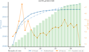
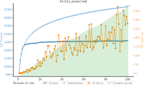
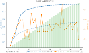
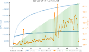
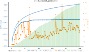
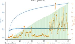
Figure 6: Applying rounds of cuts on assorted MIPLIB 2017 instances (after preprocessing) typically yields diminishing bound improvement. Several instances show a linear tendency in LP resolve time. The overlayed bar plot for each instance shows the cumulative number of cuts added after each round. The predicted bound using the improvement from the first round follows a logarithmic function that is similar to the actual bound evolution until cut strength exhibits more pronounced tailing off.

Appendix B Experiments with Optimal Proportion of Cut Rounds in SVBHC

Theorem 15 proves that, in the SVBHC model of Section 5, the number of cuts prescribed by Algorithm 1 is approximately optimal in the sense that the resulting tree is at most a multiplicative factor larger than the optimal tree size. Theorem 21 shows that using this approximately-optimal number of cuts proves a constant proportion of the overall bound, in the limit when the target bound goes to infinity. However, since the multiplicative factor in Theorem 15 may be quite large, it is not clear if the same type of limit exists for minimal-size trees. In Figure 7, we address this question computationally, showing that the proportion of bound proved by cut nodes tends to the same limit in a minimal tree for four artificial instances of the SVBHC model. Experiments with more instances have shown the same behavior and therefore are omitted.

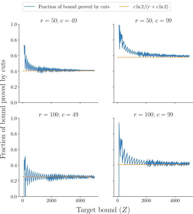
Figure 7: Fraction of bound proved by cut nodes in an (exactly-)optimal SVBHC tree, exhibiting convergence to the bound from Theorem 21 provided by the approximately-optimal number of cut nodes prescribed by Algorithm 1.

References

- [1] COIN-OR Cut Generation Library. https://github.com/coin-or/Cgl.
- [2] COIN-OR Linear Programming 1.16. https://projects.coin-or.org/Clp/.
- Achterberg and Wunderling [2013] Tobias Achterberg and Roland Wunderling. Mixed integer programming: analyzing 12 years of progress. In Facets of Combinatorial Optimization, pages 449–481. Springer, Heidelberg, 2013.
- Al-Khayyal [1987] Faiz A Al-Khayyal. An implicit enumeration procedure for the general linear complementarity problem. In Computation Mathematical Programming, pages 1–20. Springer, 1987.
- Anderson et al. [2021] Daniel Anderson, Pierre Le Bodic, and Kerri Morgan. Further results on an abstract model for branching and its application to mixed integer programming. Math. Program., 190:811–841, 2021.
- Balas et al. [2010] Egon Balas, Matteo Fischetti, and Arrigo Zanette. On the enumerative nature of gomory’s dual cutting plane method. Mathematical programming, 125(2):325–351, 2010.
- Basu et al. [2022] Amitabh Basu, Michele Conforti, Marco Di Summa, and Hongyi Jiang. Complexity of branch-and-bound and cutting planes in mixed-integer optimization – II. Combinatorica, 42(1):971–996, 2022.
- Basu et al. [2023] Amitabh Basu, Michele Conforti, Marco Di Summa, and Hongyi Jiang. Complexity of branch-and-bound and cutting planes in mixed-integer optimization. Math. Progam., 198(1):787–810, 2023.
- Berthold et al. [2022] Timo Berthold, Matteo Francobaldi, and Gregor Hendel. Learning to use local cuts, 2022. URL https://arxiv.org/abs/2206.11618.
- Burer and Vandenbussche [2008] Samuel Burer and Dieter Vandenbussche. A finite branch-and-bound algorithm for nonconvex quadratic programming via semidefinite relaxations. Math. Program., 113(2):259–282, 2008.
- Cornuéjols et al. [2011] Gérard Cornuéjols, Leo Liberti, and Giacomo Nannicini. Improved strategies for branching on general disjunctions. Math. Program., 130(2, Ser. A):225–247, 2011.
- Dey et al. [2021a] Santanu S. Dey, Yatharth Dubey, and Marco Molinaro. Branch-and-bound solves random binary packing IPs in polytime. In Dániel Marx, editor, Proceedings of the 2021 ACM-SIAM Symposium on Discrete Algorithms, SODA 2021, Virtual Conference, January 10 - 13, 2021, pages 579–591. SIAM, 2021a.
- Dey et al. [2021b] Santanu S. Dey, Yatharth Dubey, Marco Molinaro, and Prachi Shah. A theoretical and computational analysis of full strong-branching, 2021b.
- Dey et al. [2022a] Santanu S. Dey, Yatharth Dubey, and Marco Molinaro. Lower bounds on the size of general branch-and-bound trees. Math. Program., 2022a.
- Dey et al. [2022b] Santanu S. Dey, Aleksandr M. Kazachkov, Andrea Lodi, and Gonzalo Munoz. Cutting plane generation through sparse principal component analysis. SIAM J. Optim., 32(2):1319–1343, 2022b.
- Gasse et al. [2019] Maxime Gasse, Didier Chételat, Nicola Ferroni, Laurent Charlin, and Andrea Lodi. Exact combinatorial optimization with graph convolutional neural networks. In Advances in Neural Information Processing Systems, pages 15580–15592, 2019.
- Gleixner et al. [2021] Ambros Gleixner, Gregor Hendel, Gerald Gamrath, Tobias Achterberg, Michael Bastubbe, Timo Berthold, Philipp M. Christophel, Kati Jarck, Thorsten Koch, Jeff Linderoth, Marco Lübbecke, Hans D. Mittelmann, Derya Ozyurt, Ted K. Ralphs, Domenico Salvagnin, and Yuji Shinano. MIPLIB 2017: Data-Driven Compilation of the 6th Mixed-Integer Programming Library. Math. Prog. Comp., 2021.
- Gomory [1958] Ralph E. Gomory. Outline of an algorithm for integer solutions to linear programs. Bull. Amer. Math. Soc., 64:275–278, 1958.
- Gomory [1960] Ralph E. Gomory. An algorithm for the mixed integer problem. Technical Report RM-2597, RAND Corporation, 1960.
- Gomory [1963] Ralph E. Gomory. An algorithm for integer solutions to linear programs. Recent Advances in Mathematical Programming, 64:260–302, 1963.
- Gurobi Optimization, Inc. [2018] Gurobi Optimization, Inc. Gurobi Optimizer Reference Manual. http://www.gurobi.com, 2018. Version 8.0.1.
- Huang et al. [2022] Zeren Huang, Kerong Wang, Furui Liu, Hui-Ling Zhen, Weinan Zhang, Mingxuan Yuan, Jianye Hao, Yong Yu, and Jun Wang. Learning to select cuts for efficient mixed-integer programming. Pattern Recognition, 123:108353, 2022.
- Jünger et al. [2010] Michael Jünger, Thomas Liebling, Denis Naddef, George Nemhauser, William Pulleyblank, Gerhard Reinelt, Giovanni Rinaldi, and Laurence Wolsey, editors. 50 Years of Integer Programming 1958–2008. Springer-Verlag Berlin Heidelberg, 2010. From the early years to the state-of-the-art, papers from the 12th Combinatorial Optimization Workshop (Aussois 2008) held in Aussois, January 7–11, 2008.
- Karamanov and Cornuéjols [2011] Miroslav Karamanov and Gérard Cornuéjols. Branching on general disjunctions. Math. Program., 128(1-2, Ser. A):403–436, 2011.
- Kazachkov et al. [2022] Aleksandr M. Kazachkov, Pierre Le Bodic, and Sriram Sankaranarayanan. An abstract model for branch-and-cut. In Integer Programming and Combinatorial Optimization: 23rd International Conference, IPCO 2022, Eindhoven, The Netherlands, June 27–29, 2022, Proceedings, Lecture Notes in Comput. Sci., pages 333–346, Berlin, Heidelberg, 2022. Springer-Verlag.
- Khalil et al. [2016] Elias B. Khalil, Pierre Le Bodic, Le Song, George Nemhauser, and Bistra Dilkina. Learning to branch in mixed integer programming. In Thirtieth AAAI Conference on Artificial Intelligence, 2016.
- Khalil et al. [2017] Elias B. Khalil, Hanjun Dai, Yuyu Zhang, Bistra Dilkina, and Le Song. Learning combinatorial optimization algorithms over graphs. In Advances in Neural Information Processing Systems, pages 6348–6358, 2017.
- Land and Doig [1960] A. H. Land and A. G. Doig. An automatic method of solving discrete programming problems. Econometrica, 28:497–520, 1960.
- Le Bodic and Nemhauser [2017] Pierre Le Bodic and George Nemhauser. An abstract model for branching and its application to mixed integer programming. Math. Prog., 166(1-2):369–405, 2017.
- Mahajan [2009] Ashutosh Mahajan. On Selecting Disjunctions in Mixed Integer Linear Programming. PhD thesis, Lehigh University, May 2009.
- OEIS Foundation Inc. [2022] OEIS Foundation Inc. The On-Line Encyclopedia of Integer Sequences, 2022. Published electronically at https://oeis.org.
- Paulus et al. [2022] Max B Paulus, Giulia Zarpellon, Andreas Krause, Laurent Charlin, and Chris Maddison. Learning to cut by looking ahead: Cutting plane selection via imitation learning. In Kamalika Chaudhuri, Stefanie Jegelka, Le Song, Csaba Szepesvari, Gang Niu, and Sivan Sabato, editors, Proceedings of the 39th International Conference on Machine Learning, volume 162 of Proceedings of Machine Learning Research, pages 17584–17600. PMLR, 17–23 Jul 2022.
- Tang et al. [2020] Yunhao Tang, Shipra Agrawal, and Yuri Faenza. Reinforcement learning for integer programming: Learning to cut, 2020. In Proceedings of the 37th International Conference on Machine Learning (ICML 2020).
- Turner et al. [2022] Mark Turner, Thorsten Koch, Felipe Serrano, and Michael Winkler. Adaptive cut selection in mixed-integer linear programming, 2022.
- Yang et al. [2021] Yu Yang, Natashia Boland, and Martin Savelsbergh. Multivariable branching: A - knapsack problem case study. INFORMS J. Comput., 33(4):1354–1367, 2021.