Smart readout of nondestructive image sensors with single-photon sensitivity
Abstract
Image sensors with nondestructive charge readout provide single-photon or single-electron sensitivity, but at the cost of long readout times. We present a smart readout technique to allow the use of these sensors in visible-light and other applications that require faster readout times. The method optimizes the readout noise and time by changing the number of times pixels are read out either statically, by defining an arbitrary number of regions of interest (ROI) in the array, or dynamically, depending on the charge or energy of interest (EOI) in the pixel. This technique is tested in a Skipper CCD showing that it is possible to obtain deep sub-electron noise, and therefore, high resolution of quantized charge, while dynamically changing the readout noise of the sensor. These faster, low noise readout techniques show that the skipper CCD is a competitive technology even where other technologies such as Electron Multiplier Charge Coupled Devices (EMCCD), silicon photo multipliers, etc. are currently used. This technique could allow skipper CCDs to benefit new astronomical instruments, quantum imaging, exoplanet search and study, and quantum metrology.
I Introduction
Single-photon and -electron resolution semiconductor sensors have proven to be a major scientific breakthrough overcoming the limitation imposed by readout noise [1, 2, 3]. Some technologies, such as Electron Multiplying Charge Coupled Device (EMCCD) [4] or silicon photomultipliers [5], are based on charge multiplication. More recent ones use nondestructive readout techniques to average several observations of the collected charge [6, 7, 8]. Arbitrary precision is obtained at the expense of increasing the number of samples ( from here) and thus the readout time. Assuming independent measurements, the noise is reduced following [9] where is the the root mean squared error for one measurement of the charge. In particular, the Skipper CCD [9, 6] uses a floating sense node to isolate the charge packet from the first amplification stage which allows to make multiple measurements, using the correlated double sampling (CDS) method [10], to get single-electron resolution pixel readout. In recent years, many applications such as dark matter searches [11], neutrino detection [12], and study of properties of semiconductor materials [13] have exploited this capability, but others such as quantum imaging [14], astronomical terrestrial instruments [15], satellite missions for exoplanet searches [16], and sub-shot-noise microscopy [17], remain inaccessible for the Skipper CCD due to the long readout time.
The readout noise is not always the limiting factor. Other processes produce statistical fluctuations that are added in quadrature with the electronic noise and contribute to the total uncertainty. Among these processes we can mention intrinsic factors of the sensor like quantum efficiency, leakage current, charge transfer and collection inefficiencies, crystal ionization mechanism, etc; and extrinsic factors, like the Poisson statistics of photon arrival, natural background ionizing particles, etc. [18, 10]. When these dominate, there is no benefit to reducing the readout noise by increasing the readout time. In this article a smart readout technique to reduce readout time by changing the readout noise based on available information for the specific application is presented. Experimental results using an Skipper CCD are reported, but the technique may be also applied to any existing or future sensors with nondestructive readout (either with active or passive pixels) to adapt either the readout time or the dynamic range of the measuring system.
II Description of the technique
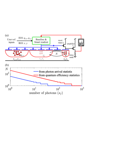
Figure 1(a) shows a conceptual diagram. The block “baseline and smart readout” confers intelligence to the output stage of the CCD to perform an adaptive modification of the number of measurements of the charge in each pixel using information of the sensor’s parameters, the physics source of interest (reference inputs) and information of the current pixel. The easier strategy is to optimize according to the position of the pixel in the array (). If the incoming photon flux illuminates a specific region, can be increased for that region, while faster readout (and higher noise) can be used for the remaining area. This strategy adjusts the readout time and noise (or equivalently, adjusts the dynamic range) based on regions of interest (ROI) which are previously known for the application. Another approach is to update depending on the range of charge () or deposited energy being measured, i.e. based on the energy of interest (EOI).
For example, typical applications currently limited for the Skipper CCD involve visible or infrared light detection. These systems are intrinsically limited by photon statistics, which can be described by a binomial distribution (attributed to the collection efficiency of the detector) together with a Poisson distribution (attributed to photon arrival statistics).
Two scenarios are considered to show the EOI strategy: 1) a system limited by Poisson uncertainty of photon arrival, as any astronomical instrument [19], assuming ideal collection of photons in the sensor; 2) a system limited by photon detection uncertainty, due to quantum efficiency (), following a binomial distribution and assuming no Poisson arrival uncertainty, as expected in applications using entangled photons [20]. In both systems, the signal to noise ratio (SNR) is , where is the expected number of collected photons and is the standard deviation in the expected number of collected photons ( and for each example respectively). The number of samples per pixel can be tuned to get a desired SNR for each number of collected photons (or equivalently collected charge). If is adjusted to produce a SNR for each pixel equal to times () its SNR without readout noise (=0), so that the fractional contribution of readout noise to photon uncertainty is the same for every pixel, then,
| (1) |
As shown in Fig. 1(b), increasing significantly decreases the uncertainty on the number of collected photons for pixels collecting fewer than photons for Poisson statistics and for binomial statistics. For pixels with more than this number of photons, (1) finds that is sufficient to meet the goal defined by .
This shows that an smart strategy has a big potential in reducing the readout time and tuning the dynamic range of the system for pixels with relatively small charge packets (% and % of the full pixel capacity, as tested for similar devices [21]) which demands larger values to meet the SNR requirement. For a general application, assuming a uniform distribution of pixel charge values between 1 and , the result in Fig. 1(b) gives that the readout time with a smart strategy is and that of the non-smart strategy (all pixels read out with the highest value), in the Poisson and binomial scenarios respectively.
III Implementation challenges
Although changing the number of samples read per pixel seems straightforward, this requires changing the clock signals (twenty in our case) of the CCD “on the fly.” Because the CCD is a highly coupled device and the voltage swings of the clocks are on the order of tens of volts, changes to the clocks cause variations in the baseline of the video signal that, if not treated properly, introduce a systematic error in the determination of the pixel charge. Since the sensitivity of the CCD is in the order of 2V, this imposes a sub-ppm control of the errors. We develop a calibration technique that can be performed on- and off-line so that can be changed without increasing the systematic error due to baseline variation.
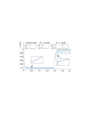
Figure 2 shows a measurement of the baseline changes in the raw video signal, before pixel computation, due to the changing clocks signals applied to a skipper CCD. The exponential decay at is caused by the vertical clocks applied before . The plateau that follows is caused by many consecutive pixels read out with . The slope within a single pixel, seen in the inset, will cause a non-zero pixel value, an effect that is present in every CCD. The exponential at is caused by a change in the readout mode, from to . The downward glitches seen for correspond to the first measurement of each pixel, which has a different clocking compared to the next measurements. Figure 2 shows a change of V in the output signal base level (baseline), which exceeds by times the expected signal for one electron ( 2V).
Baseline is present in any CCD; it is usually estimated by taking an overscan region (empty pixels obtained by reading more charge packets from the serial register than there are active pixels), and subtracted from each image [22]. A similar approach can be used for the ROI strategy [23], though this requires extra calibration time to acquire empty images for each ROI. On the other hand, the EOI strategy changes online and requires corrected pixel values to be available during readout. Therefore it is mandatory to have a baseline compensation technique that can be applied online.
We developed a baseline correction technique based on the superposition of the effects of a group of control signals on the output video signal. An identification procedure is performed only once, and the baseline correction can be computed (online and offline) as the superposition of the calibrated effects for any readout sequence, either under ROI or EOI. The identification procedure is performed in the pixel values and not in the raw video signal, thus simplifying the implementation as discussed in the supplemental material [24].
IV Experimental results
The experimental proof of concept of the technique is done switching between and for ROI and EOI experiments. results in deep sub-electron noise operation and therefore any artifact introduced by the proposed adaptive readout would impact the measured total noise. Also, the jump between or produces a large change in the baseline allowing to test the capability of the readout routine to compensate for these perturbations.
Inside a dewar, the skipper-CCD is operated at high vacuum (approximately mbar) and at a temperature of K. The sensor is a fully-depleted CCD developed by Lawrence Berkeley National Laboratory, LBNL [6]. The low threshold acquisition controller (LTA) [25] is used for readout and control.
We report three experiences: 1) ROI specified before the readout, 2) EOI experiment choosing different charge ranges and 3) a combination of both: once a pixel is detected in EOI, a ROI to the right of that pixel is readout with large to achieve sub-electron noise.
For the online implementation of the EOI: the first measurement of the pixel is corrected by the baseline algorithm. If the value is within the charge range set by the user, further samples are taken of the same pixel. However, if the first value is outside the range, the readout sequence continues with the next pixel. The complete baseline compensation is applied to the final image. For the ROI strategy the compensation is only applied to the final image. Further details can be found in the supplemental material [24].
IV.0.1 Experiment with ROI
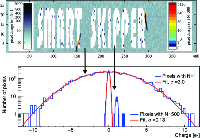
Fig. 3 shows an image acquired with the proposed ROI technique. To show the versatility, ROIs were defined by the words “SMART SKIPPER”: noise is 0.13 inside the letters and 3 outside. Both noise measurements are obtained by Gaussian fits of the histograms, as shown in the figure. This is the theoretical expected reduction of noise when going from to : which proves that that the baseline compensation technique does not harm the sensor charge resolution.
IV.0.2 Experiment with EOI
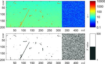
Figure 4 show an image taken with the proposed technique after a long exposure time to collect charge from intrinsic ionization in the sensor, with for pixels with 0 to 42 and for pixels with or . Two notable regions are observed: part of the active region of the sensor with interacting particles and an overscan region starting in column . The resulting pattern of Skipper samples is depicted at the bottom. Due to the long exposure, most of the active region is modestly charged and therefore read with . The exception are the energetic muon and electron tracks, where most pixels have charge greater than 42 and are automatically read with . In the overscan region mostly empty pixels are present resulting in a random pattern of and and showing the versatility of the system to change the value of in every pixel.
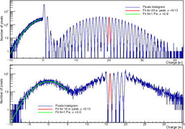
Figure 5 shows two histograms in logarithmic scale as a result of applying the EOI technique in two different experiments. Peaks at integer numbers of electrons are clearly observed in two different charge intervals where charge quantization is achieved using .
In both measurements, the envelope of the histograms has two distinctive bumps, one around 0 from mostly empty pixels (mainly from the overscan) and another one centered at approximately 20 (from the active region). The latter shows, in logarithmic scale, the characteristic Poisson distribution.
A half Gaussian distribution is observed at the left of 0 in the histogram at the top. The green line shows a fit with a standard deviation , which is the expected readout noise for . For the results are depicted in red with a fit of the 20 peak. The standard deviation of the fit is , again verifying the theoretical prediction for independent averaged measurements despite changing dynamically based on the pixel charge. The histogram at the bottom, for charge in the interval 15 to 19, also shows the Gaussian fitting and the same noise performance.
IV.0.3 Experiment combining ROI and EOI
We combine both ROI and EOI techniques using the ionization produced by a muon track to trigger sub-electron pixel measurement.
The charge range is set between and to avoid false trigger from dark current generation. If the charge of a pixel is in the range, the current and the following pixels are read times, independent of their charge value.
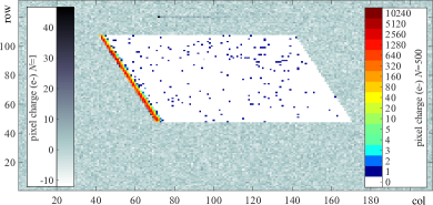
Figure 6 shows a fraction of the image where a muon was detected (straight line). The muon is seen mostly in red colors indicating hundreds or thousands of electrons deposited in those pixels. To the right of the muon, pixels were also read with samples per pixel; those pixels are observed as a white parallelogram ROI composed mostly of empty pixels (white pixels) and some pixels with .
This experiment shows that it is possible to combine both techniques, which could be useful to study the charge generation around certain events of interest.
V Scientific Applications
New astronomical instruments
The potential of the sub-electron noise of the Skipper CCD is being explored for terrestrial astronomy [6, 15] for signals with small SNR. Acquisitions with limited exposure time naturally produce low SNR observations where the impact of readout noise is high. Authors claim that a reduction of in the readout time is still required, which is similar to the time reduction obtained by EOI in previous section in systems limited by photon arrival statistics. Moreover, for spectrography instruments where spectra are well defined areas in the sensor [26], a ROI strategy could further improve the readout speed. To quantitatively address this scenario we obtained a real image from the LDSS-3 [T. Diehl 2018, private communication], a high efficiency optical wide-field imager and multi-slit spectrograph [27]. The value for each pixel based on the Poisson uncertainty was computed and resulted in a reduction of the readout time of a factor of .
Quantum imaging techniques
A pair of photons can exhibit spatial, spectral and polarization quantum entanglement. Spatial entanglement has been extensively explored for quantum communication [28]. Spontaneous parametric down-conversion crystals have eased the production of entangled pairs over a large number of positions [29] for example for ghost imaging [30, 31]. Intensity correlation can be used for several other imaging techniques [32] such as fluorescence correlation spectroscopy [33]. Two-dimensional semiconductor devices provide a good sensor solution for these applications [34]. In particular, the single photon counting capability and large quantum efficiency of the Skipper CCD make it a promising technology in the field [14]. Moreover, as detailed in [32] on-chip noise sources impact the final measurable correlation of entangled photons, and therefore the EOI and ROI strategies can be used due to the high spatial and intensity correlation between entangled photons in two known regions of the image.
Exoplanet search and study
Direct imaging space telescopes for exoplanet detection and characterization are being planned [35]. One of the main goals for future missions is to search for near-infrared photons at nm from water vapor in the atmosphere of potentially habitable planets. A sensor with large quantum efficiency and sub-electron readout noise is required. The Skipper CCD has been identified by NASA as a promising technology that meets both requirements [16, 36, 35]. Moreover, the radiation hardness compared to EMCCD makes it more suitable for space missions. The main identified challenge is the slow readout time ( minutes for Mpixel array read by one amplifier at deep sub-electron noise). According to [37] less than 200 hundred pixels per spectral element will be needed for the mission’s spectrograph. To overcome the readout time limitation one possibility is to use the ROI strategy to directly focus on the key wavelengths and meet the 20 second readout time constraint [36].
Electron pump for quantum metrology
Recently there has been a redefinition of the ampere by means of the charge of the electron [38, 39]. One of the technological candidates for metrology is the single-electron transistor (SET) [40]. These quantum devices are operated at milli-Kelvin temperatures, which complicates the scaling required to achieve reasonable practical currents (in the order of A). The Skipper CCD is a promising technology for the development of a current source with single-electron manipulation. Although scaling is still a challenge, one advantages is its higher temperature of operation (in the order of Kelvin). To reach an stable average current a smart readout technique is mandatory, since charge should be measured and drained out of the device at a rate that depends on the actual charge packet measurement [41].
Acknowledgements.
We thank the SiDet team at Fermilab for the support on the operations of CCDs and Skipper-CCDs, especially Kevin Kuk and Andrew Lathrop. Lawrence Berkeley National Laboratory is the developer of the fully-depleted CCD and the designer of the Skipper readout. The CCD development work was supported in part by the Director, Office of Science, of the U.S. Department of Energy under No. DE-AC02-05CH11231.References
- Simoen and Claeys [1999] E. Simoen and C. Claeys, Solid-State Electronics 43, 865 (1999).
- Janesick et al. [1990] J. R. Janesick, T. S. Elliott, A. Dingiziam, R. A. Bredthauer, C. E. Chandler, J. A. Westphal, and J. E. Gunn, in Charge-Coupled Devices and Solid State Optical Sensors, Vol. 1242, edited by M. M. Blouke, International Society for Optics and Photonics (SPIE, 1990) pp. 223 – 237.
- Boukhayma [2017] A. Boukhayma, Ultra Low Noise CMOS Image Sensors, Springer Theses (Springer International Publishing, 2017).
- Hynecek and Nishiwaki [2003] J. Hynecek and T. Nishiwaki, IEEE Transactions on Electron Devices 50, 239 (2003).
- Buzhan et al. [2003] P. Buzhan, B. Dolgoshein, L. Filatov, A. Ilyin, V. Kantzerov, V. Kaplin, A. Karakash, F. Kayumov, S. Klemin, E. Popova, and S. Smirnov, Nuclear Instruments and Methods in Physics Research Section A: Accelerators, Spectrometers, Detectors and Associated Equipment 504, 48 (2003), proceedings of the 3rd International Conference on New Developments in Photodetection.
- Tiffenberg et al. [2017] J. Tiffenberg, M. Sofo-Haro, A. Drlica-Wagner, R. Essig, Y. Guardincerri, S. Holland, T. Volansky, and T.-T. Yu, Phys. Rev. Lett. 119, 131802 (2017), 1706.00028 .
- Stefanov et al. [2020] K. D. Stefanov, M. J. Prest, M. Downing, E. George, N. Bezawada, and A. D. Holland, Sensors 20, 2031 (2020).
- Bautz et al. [2019] M. W. Bautz, B. E. Burke, M. Cooper, D. Craig, R. F. Foster, C. E. Grant, B. J. LaMarr, C. Leitz, A. Malonis, E. D. Miller, G. Prigozhin, D. Schuette, V. Suntharalingam, and C. Thayer, Journal of Astronomical Telescopes, Instruments, and Systems 5, 1 (2019).
- Fernandez Moroni et al. [2012] G. Fernandez Moroni, J. Estrada, G. Cancelo, S. Holland, E. Paolini, and H. Diehl, Experimental Astronomy 34 (2012), 10.1007/s10686-012-9298-x.
- Janesick [2001] J. R. Janesick, Scientific charge-coupled devices, Vol. 83 (SPIE press, 2001).
- Barak et al. [2020] L. Barak, I. M. Bloch, M. Cababie, G. Cancelo, L. Chaplinsky, F. Chierchie, M. Crisler, A. Drlica-Wagner, R. Essig, J. Estrada, E. Etzion, G. F. Moroni, D. Gift, S. Munagavalasa, A. Orly, D. Rodrigues, A. Singal, M. S. Haro, L. Stefanazzi, J. Tiffenberg, S. Uemura, T. Volansky, and T.-T. Yu (SENSEI Collaboration), Phys. Rev. Lett. 125, 171802 (2020).
- D’Olivo et al. [2020] J. C. D’Olivo, C. Bonifazi, D. Rodrigues, and G. F. Moroni, in XXIX International Conference in Neutrino Physics, poster 521 (2020).
- Rodrigues et al. [2020] D. Rodrigues, K. Andersson, M. Cababie, A. Donadon, G. Cancelo, J. Estrada, G. Fernandez-Moroni, R. Piegaia, M. Senger, M. S. Haro, et al., arXiv preprint arXiv:2004.11499 (2020).
- Estrada et al. [2021] J. Estrada, R. Harnik, D. Rodrigues, and M. Senger, “Ghost imaging of dark particles,” (2021), arXiv:2012.04707 [hep-ph] .
- Drlica-Wagner et al. [2020] A. Drlica-Wagner, E. M. Villalpando, J. O’Neil, J. Estrada, S. Holland, N. Kurinsky, T. Li, G. F. Moroni, J. Tiffenberg, and S. Uemura, in X-Ray, Optical, and Infrared Detectors for Astronomy IX, Vol. 11454, edited by A. D. Holland and J. Beletic, International Society for Optics and Photonics (SPIE, 2020) pp. 210 – 223.
- Rauscher et al. [2019] B. J. Rauscher, S. E. Holland, L. R. Miko, and A. Waczynski, in UV/Optical/IR Space Telescopes and Instruments: Innovative Technologies and Concepts IX, Vol. 11115, edited by A. A. Barto, J. B. Breckinridge, and H. P. Stahl, International Society for Optics and Photonics (SPIE, 2019) pp. 382 – 386.
- Samantaray et al. [2017] N. Samantaray, I. Ruo-Berchera, A. Meda, and M. Genovese, Light: Science & Applications 6, e17005 (2017).
- Groom et al. [1999] D. E. Groom, S. E. Holland, M. E. Levi, N. P. Palaio, S. Perlmutter, R. J. Stover, and M. Wei, in Sensors, Cameras, and Systems for Scientific/Industrial Applications, Vol. 3649, edited by M. M. Blouke and G. M. W. Jr., International Society for Optics and Photonics (SPIE, 1999) pp. 80 – 90.
- Janesick and of Physics [2007] J. Janesick and A. I. of Physics, Photon Transfer: DN [lambda] (SPIE, 2007).
- Brida and Ruo Berchera [2010] G. Brida and I. Ruo Berchera, Nature Photonics 4, 227 (2010).
- Diehl et al. [2008] H. T. Diehl, R. Angstadt, J. Campa, H. Cease, G. Derylo, J. H. Emes, J. Estrada, D. Kubik, B. L. Flaugher, S. E. Holland, M. Jonas, W. F. Kolbe, J. Krider, S. Kuhlmann, K. Kuk, M. Maiorino, N. Palaio, A. Plazas, N. A. Roe, V. Scarpine, K. Schultz, T. Shaw, H. Spinka, and W. Stuermer, in High Energy, Optical, and Infrared Detectors for Astronomy III, Vol. 7021, edited by D. A. Dorn and A. D. Holland, International Society for Optics and Photonics (SPIE, 2008) pp. 86 – 96.
- Roundy [1997] C. B. Roundy, in 10th Meeting on Optical Engineering in Israel, Vol. 3110, edited by I. Shladov and S. R. Rotman, International Society for Optics and Photonics (SPIE, 1997) pp. 860 – 879.
- Chierchie et al. [2020] F. Chierchie, G. F. Moroni, L. Stefanazzi, C. Chavez, E. Paolini, G. Cancelo, M. S. Haro, J. Tiffenberg, J. Estrada, and S. Uemura, “Smart-readout of the skipper-ccd: Achieving sub-electron noise levels in regions of interest,” (2020), arXiv:2012.10414 [physics.ins-det] .
- [24] SUPPLEMENTAL MATERIALS for: Smart readout of nondestructive image sensors with single-photon sensitivity.
- Cancelo et al. [2021] G. I. Cancelo, C. Chavez, F. Chierchie, J. Estrada, G. Fernandez-Moroni, E. E. Paolini, M. S. Haro, A. Soto, L. Stefanazzi, J. Tiffenberg, K. Treptow, N. Wilcer, and T. J. Zmuda, Journal of Astronomical Telescopes, Instruments, and Systems 7, 1 (2021).
- Howell [2006] S. B. Howell, Handbook of CCD astronomy, Vol. 5 (Cambridge University Press, 2006).
- LDSS3 [2021] LDSS3, The Low Dispersion Survey Spectrograph (2021(accessed October 19, 2021)), http://www.lco.cl/wp-content/uploads/2021/02/LDSS3handout2021.pdf.
- Yuan et al. [2010] Z.-S. Yuan, X.-H. Bao, C.-Y. Lu, J. Zhang, C.-Z. Peng, and J.-W. Pan, Physics Reports 497, 1 (2010).
- Malygin et al. [1985] A. A. Malygin, A. N. Penin, and A. V. Sergienko, Soviet Physics Doklady 20, 227 (1985).
- Padgett and Boyd [2017] M. J. Padgett and R. W. Boyd, Philosophical Transactions of the Royal Society A: Mathematical, Physical and Engineering Sciences 375, 20160233 (2017).
- Pittman et al. [1995] T. B. Pittman, Y. H. Shih, D. V. Strekalov, and A. V. Sergienko, Phys. Rev. A 52, R3429 (1995).
- Defienne et al. [2018] H. Defienne, M. Reichert, and J. W. Fleischer, Phys. Rev. Lett. 120, 203604 (2018).
- Bestvater et al. [2010] F. Bestvater, Z. Seghiri, M. Kang, N. Gröner, J.-Y. Lee, K.-B. Im, and M. Wachsmuth, Optics express 18, 23818 (2010).
- Orieux et al. [2017] A. Orieux, M. A. M. Versteegh, K. D. Jöns, and S. Ducci, Reports on Progress in Physics 80, 076001 (2017).
- Crill and Siegler [2018] B. Crill and N. Siegler, Jet Propulsion Laboratory Publications D-102506 (2018).
- [36] B. J. Rauscher, S. E. Holland, L. R. Miko, and A. Waczynski, .
- Stark et al. [2019] C. Stark, R. Belikov, M. Bolcar, B. Crill, J. Krist, B. Nemati, L. Pueyo, B. Rauscher, A. J. E. Riggs, G. Ruane, D. Sirbu, R. Soummer, K. St. Laurent, N. Zimmerman, and T. Groff, in American Astronomical Society Meeting Abstracts #233, American Astronomical Society Meeting Abstracts, Vol. 233 (2019) p. 402.05.
- des Poids et Mesure [2019] B. I. des Poids et Mesure, Mise en pratique for the definition of the ampere and other electric units in the SI (2019), appendix 2.
- Scherer and Schumacher [2019] H. Scherer and H. W. Schumacher, Annalen der Physik 531, 1800371 (2019).
- Giblin et al. [2012] S. Giblin, M. Kataoka, J. Fletcher, P. See, T. Janssen, J. Griffiths, G. Jones, I. Farrer, and D. Ritchie, Nature communications 3, 1 (2012).
- Tiffenberg and Moroni [2021] J. Tiffenberg and G. F. Moroni, Pinning down the ampere with a supersensitive particle detector (2020 (accessed April 29, 2021)), https://news.fnal.gov/2020/10/pinning-down-the-ampere-with-a-supersensitive-particle-detector/.