Rate-optimal Bayesian Simple Regret in Best Arm Identification

Abstract

We consider best arm identification in the multi-armed bandit problem. Assuming certain continuity conditions of the prior, we characterize the rate of the Bayesian simple regret. Differing from Bayesian regret minimization (Lai, 1987), the leading term in the Bayesian simple regret derives from the region where the gap between optimal and suboptimal arms is smaller than $\sqrt{\frac{\log T}{T}}$. We propose a simple and easy-to-compute algorithm with its leading term matching with the lower bound up to a constant factor; simulation results support our theoretical findings.

1 Introduction

We consider finding the best treatment among $K$ and $T$ sample size. In this problem, each arm (treatment) $i\in[K]=\{1,2,\dots,K\}$ is associated with (unknown) parameter $\mu_{i}\in[0,1]$. We use $\bm{\mu}=(\mu_{1},\mu_{2},\dots,\mu_{K})$ to denote the set of parameters. At each round $t=1,2,\dots,T$, the forecaster, who follows some adaptive algorithm, selects an arm $I(t)\in[K]$ and receives the corresponding reward $X_{I(t)}(t)\sim\mathrm{Bernoulli}(\mu_{I(t)})$, where $1$ and $0$ represent the success and the failure of the selected treatment. Let $i^{*}=\operatorname*{arg\,max}_{i}\mu_{i}$ and $\mu^{*}=\mu_{i^{*}}$ be the optimal (best) arm and its corresponding mean, respectively.

The existing literature has mainly considered two different objectives. The first involves maximizing the total reward (Robbins,, 1952; Lai and Robbins,, 1985), which is equivalent to minimizing the draw of suboptimal arms. Letting $N_{i}(T)$ be the number of draws on arm $i$ up to round $T$, the (frequentist) regret is defined as

$$\mathrm{Reg}_{\bm{\mu}}(T):=\sum_{i=1}^{K}\mathbb{E}_{\bm{\mu}}[N_{i}(T)](\mu^{*}-\mu_{i}),$$ (1)

where $\bm{\mu}$ is unknown but fixed, and the expectation here is over the randomness of the rewards and (possibly randomized) choices $I(t)$.

The second objective is identifying the best arm. In this case, the forecaster at the end of round $T$ recommends an arm $J(T)$. The performance of the forecaster is measured by the simple regret

$$\mathrm{R}_{\bm{\mu}}(T):=\mu^{*}-\mathbb{E}_{\bm{\mu}}[\mu_{J(T)}],$$ (2)

which is the expected difference between the means of the best arm and recommended arm $J(T)$. The two objectives are very different. Minimizing regret (Eq. (1)) requires balancing the exploration (i.e., drawing all arms to obtain more information) and the exploitation (i.e., obtaining more rewards by drawing an empirically good arm). On the other hand, in minimizing simple regret, the rewards from the arms $I(t)$ ($1\leq t\leq T$) are not considered. Therefore, Eq. (2) is minimized by pure exploration (Bubeck et al.,, 2011).

The simple regret of Eq. (2) is frequentist; it assumes that $\bm{\mu}$ is (unknown but) fixed. On the other hand, we may consider a distribution of $\bm{\mu}\in[0,1]^{K}$ and take the expectation of the frequentist simple regret over the distribution. We can call this the Bayesian simple regret, which is defined as

$$\mathrm{R}_{H}(T) =\mathbb{E}_{\bm{\mu}\sim H}[\mathrm{R}_{\bm{\mu}}(T)],$$ (3)

where $\mathbb{E}_{\bm{\mu}\sim H}$ marginalizes $\bm{\mu}$ over the prior $H$ on $[0,1]^{K}$. In this paper, we consider the problem of minimizing the Bayesian simple regret of Eq. (3). We drop the term “Bayesian” when it clearly refers to Bayesian simple regret.

1.1 Regularity condition

We assume the following regularity condition for the prior distribution. For $i\in[K]$, let $\bm{\mu}_{\setminus i}$ be the set of $K-1$ parameters other than $\mu_{i}$. For $i,j\in[K]$, let $\bm{\mu}_{\setminus ij}$ be the set of $K-2$ parameters other than $\mu_{i},\mu_{j}$. Let $H_{\setminus i}(\bm{\mu}_{\setminus i})$ be the joint cumulative density function of $\bm{\mu}_{\setminus i}$, and $H_{i}(\mu_{i}|\bm{\mu}_{\setminus i})$ be the conditional cumulative density function of $\mu_{i}$ given $\bm{\mu}_{\setminus i}$. Define $H_{\setminus ij}(\bm{\mu}_{\setminus ij})$, $H_{ij}(\mu_{i},\mu_{j}|\bm{\mu}_{\setminus ij})$ in the same way. The following assumption concerns the existence of continuous derivatives of $H_{i}(\mu_{i}|\bm{\mu}_{\setminus i})$ and $H_{ij}(\mu_{i},\mu_{j}|\bm{\mu}_{\setminus ij})$.

Assumption 1.

(Uniform continuity of the conditional probability density functions) There exist conditional probability density functions $h_{i}(\mu_{i}|\bm{\mu}_{\setminus i})$ and $h_{ij}(\mu_{i},\mu_{j}|\bm{\mu}_{\setminus ij})$ that are uniformly continuous. Namely, for every $\epsilon>0$ there exists $\delta=\delta(\epsilon)>0$ such that

$$\forall\,|\mu_{i}-\lambda_{i}|\leq\delta, \quad|h_{i}(\mu_{i}|\bm{\mu}_{\setminus i})-h_{i}(\lambda_{i}|\bm{\mu}_{\setminus i})|\leq\epsilon,$$

$$\forall\,|\mu_{i}-\lambda_{i}|,|\mu_{j}-\lambda_{j}|\leq\delta, \quad|h_{ij}(\mu_{i},\mu_{j}|\bm{\mu}_{\setminus ij})-h_{ij}(\lambda_{i},\lambda_{j}|\bm{\mu}_{\setminus ij})|\leq\epsilon.$$ (4)

Remark 1.

(Uniform continuity) Assumption 1 is similar to that of Lai, (1987); however, it is slightly stronger. Namely, we assume the uniform continuity; $\delta$ in Eq. (4) does not depend on $\bm{\mu}$. We also assume the uniform continuity of $h_{ij}(\mu_{i},\mu_{j}|\bm{\mu}_{\setminus ij})$, which is required to bound the probability that three or more arms have very similar means.

We consider Assumption 1 to be satisfied by most distributions of interests. For example, it is satisfied when the joint distribution is Lipschitz continuous, as in the case that each $\mu_{i}$ is drawn from the uniform prior and not very strongly correlated with each other. However, the following demonstrates a situation in which Assumption 1 does not hold.

Example 1.

(Corner case excluded by Assumption 1) Let there be three arms. Parameters $\mu_{1},\mu_{2}\sim\mathrm{Unif}(0,1)$ are independent each other, and $\mu_{3}=1-\mu_{1}$. That is, the parameters are redundant. This case violates Assumption 1 because $h_{3}(\mu_{3}|\mu_{1},\mu_{2})$ has point mass on $1-\mu_{1}$ and is not continuous.

Note also that we assume that the prior $H$ is independent of $T$. In appendix, we describe another example in which $H$ is dependent on $T$ (Section A in the appendix).

1.2 Main results

Table 1 compares our results and existing results. Subsequently, we characterize the optimal rate of the Bayesian simple regret.

Table 1: Optimal rate in regret minimization (RM) setting and simple regret minimization (SRM) setting. The optimality presented in each column indicates that the leading factor of the corresponding measure (RM or SRM) matches the lower bound.

	RM	SRM
Frequentist	$\Theta(\log T)$ Lai and Robbins, (1985)	$\Theta(\exp(-\Gamma T))$ Carpentier and Locatelli, (2016) (up to a constant)
Bayesian	$\Theta((\log T)^{2})$ Lai, (1987)	$\Theta(T^{-1})$ This paper (up to a constant)

According to Theorem 3 of Lai, (1987), an asymptotically optimal algorithm’s Bayesian regret is

$$\mathrm{Reg}_{H}(T):=\mathbb{E}_{\bm{\mu}\sim H}[\mathrm{Reg}_{\bm{\mu}}(T)]=\frac{(\log T)^{2}}{2}\sum_{i=1}^{K}\int_{[0,1]^{K-1}}h_{i}(\mu_{\setminus i}^{*}|\bm{\mu}_{\setminus i})dH_{\setminus_{i}}(\bm{\mu}_{\setminus i})+o((\log T)^{2}),$$ (5)

where $\mu_{\setminus i}^{*}=\max_{j\neq i}\mu_{j}$.

This paper shows that the expected Bayesian simple regret is bounded as

$$\mathrm{R}_{H}(T)\leq\frac{1}{T}\sum_{i=1}^{K}\int_{[0,1]^{K-1}}\mu_{\setminus i}^{*}(1-\mu_{\setminus i}^{*})h_{i}(\mu_{\setminus i}^{*}|\bm{\mu}_{\setminus i})dH_{\setminus i}(\bm{\mu}_{\setminus i})+o\left(\frac{1}{T}\right)$$ (6)

and derives the corresponding lower bound that matches the upper bound up to a (universal) constant factor. That is, we characterize the optimal rate of the Bayesian simple regret under the continuity assumption of the prior.

Among the greatest challenges for establishing the Bayesian simple regret bound is the absence of any notion for characterizing “good” algorithm. In the case of regret minimization (RM), Lai and Robbins, (1985) proposed a notion of “uniformly good”; an algorithm is uniformly good if it has $o(T^{c})$ regret for any $c>0$ and for any fixed parameter $\bm{\mu}$. Almost all meaningful algorithms in RM setting are uniformly good. The bound of Eq. (5) can be explained by (some of) the asymptotically optimal algorithms among the uniformly good algorithms. In contrast, an optimal algorithm in the context of Bayesian simple regret minimization (SRM) remains relatively unexplored. Although certain frequentist characterizations are known (Audibert et al.,, 2010; Carpentier and Locatelli,, 2016), there are currently no notions that correspond to RM’s notions of “uniformly good” or “asymptotical optimality.” Accordingly, this paper demonstrates that a minimal assumption on the prior distribution can be sufficient to derive the asymptotic rate of the Bayesian simple regret.

1.3 Intuitive derivation of the bound

This section provides an informal derivation of Eq. (6). Section 2 presents the formal results.

Consider the parameters $\bm{\mu}:\mu_{i}>\mu_{\setminus i}^{*}$ where arm $i$ is the best arm. The Kullback-Leibler (KL) divergence between parameters $(\mu_{i},\mu_{\setminus i}^{*})$ and $(\frac{\mu_{\setminus i}^{*}+\mu_{i}}{2},\frac{\mu_{\setminus i}^{*}+\mu_{i}}{2})$ characterizes the difficulty of confirming that $\mu_{i}$ is larger than $\mu_{\setminus i}^{*}$. That is, the frequentist simple regret for parameter $\bm{\mu}$ is approximately

$$\frac{\mu_{i}-\mu_{\setminus i}^{*}}{2}\exp\left(-Td_{\mathrm{KL}}\left(\mu_{\setminus i}^{*},\frac{\mu_{\setminus i}^{*}+\mu_{i}}{2}\right)\right),$$ (7)

where $d_{\mathrm{KL}}(p,q)=p\log(p/q)+(1-p)\log((1-p)/(1-q))$ is the KL divergence between two Bernoulli distributions with parameters $p,q\in(0,1)$. Integrating this over the prior yields

$$\int_{[0,1]^{K-1}}\int_{(\mu_{\setminus i}^{*},1]}\frac{\mu_{i}-\mu_{\setminus i}^{*}}{2}\exp\left(-Td_{\mathrm{KL}}\left(\mu_{\setminus i}^{*},\frac{\mu_{\setminus i}^{*}+\mu_{i}}{2}\right)\right)h_{i}(\mu_{i}|\bm{\mu}_{\setminus i})d\mu_{i}dH_{\setminus_{i}}(\bm{\mu}_{\setminus i})$$ (8)

$$\approx\int_{[0,1]^{K-1}}\int_{(\mu_{\setminus i}^{*},\mu_{\setminus i}^{*}+O(\sqrt{\frac{\log T}{T}})]}\frac{\mu_{i}-\mu_{\setminus i}^{*}}{2}\exp\left(-Td_{\mathrm{KL}}\left(\mu_{\setminus i}^{*},\frac{\mu_{\setminus i}^{*}+\mu_{i}}{2}\right)\right)h_{i}(\mu_{\setminus i}^{*}|\bm{\mu}_{\setminus i})d\mu_{i}dH_{\setminus_{i}}(\bm{\mu}_{\setminus i})$$ (9)

     (continuity implies $$h_{i}(\mu_{i}|\bm{\mu}_{\setminus i})\approx h_{i}(\mu_{\setminus i}^{*}|\bm{\mu}_{\setminus i}) \mu_{i}-\mu_{\setminus i}^{*}=O(\sqrt{(\log T)/T})=o(1)$$ when ) (10)

$$\approx\int_{[0,1]^{K-1}}\left[-\frac{2\mu_{\setminus i}^{*}(1-\mu_{\setminus i}^{*})}{T}\exp\left(-Td_{\mathrm{KL}}\left(\mu_{\setminus i}^{*},\frac{\mu_{\setminus i}^{*}+\mu_{i}}{2}\right)\right)\right]_{\mu_{\setminus i}^{*}}^{\mu_{\setminus i}^{*}+O(\sqrt{\frac{\log T}{T}})}h_{i}(\mu_{\setminus i}^{*}|\bm{\mu}_{\setminus i})dH_{\setminus_{i}}(\bm{\mu}_{\setminus i})$$ (11)

$$=\int_{[0,1]^{K-1}}\frac{2\mu_{\setminus i}^{*}(1-\mu_{\setminus i}^{*})}{T}h_{i}(\mu_{\setminus i}^{*}|\bm{\mu}_{\setminus i})dH_{\setminus_{i}}(\bm{\mu}_{\setminus i})+o\left(\frac{1}{T}\right),$$ (12)

which is twice as Eq. (6). A more elaborated analysis removes the factor of two and yields Eq. (6). The derivation implies

• The region that matters is $\mu_{i}-\mu_{\setminus i}^{*}=O(1/\sqrt{T})=o(\sqrt{(\log T)/T})$, which is small when $T$ is large. By Assumption 1, $h_{i}(\mu_{i}|\bm{\mu}_{\setminus i})$ is sufficiently flat in this region.

• Let ${\setminus i}^{*}$ be the second best arm. When $|\mu_{i}-\mu_{\setminus i}^{*}|\approx O(1/\sqrt{T})$ and the arms other than $i,{\setminus i}^{*}$ are substantially suboptimal, the optimal strategy invests most of the $T$ rounds into the two arms. Eq. (7) represents the information-theoretic bound of identifying the parameters $(\mu_{i},\mu_{\setminus i}^{*})$ (i.e., arm $i$ is better) from $(\frac{\mu_{\setminus i}^{*}+\mu_{i}}{2},\frac{\mu_{\setminus i}^{*}+\mu_{i}}{2})$ (i.e., both arms are the same).

• The term $\mu_{\setminus i}^{*}(1-\mu_{\setminus i}^{*})$ implies that the closer the best arm to $0,1$, the more identifiable it is. This is intuitive because the KL divergence diverges around $0,1$ in Bernoulli distributions.

1.4 Related work

The multi-armed bandit (MAB) problem has garnered much attention in the machine learning community because it is useful in several crucial applications such as online advertisements and A/B testings. The goal of the standard MAB problem is to maximize the sum of the rewards, which boils down to regret minimization (RM). On the other hand, there is another established branch of bandit problems, called best arm identification (BAI, Audibert et al., (2010)). In BAI, the goal is to find the arm with the highest expected reward; this is closely related to the classical sequential tests (Chernoff,, 1959). Maximizing the mean quality of the recommendation arm $J(T)$ boils down to simple regret minimization (SRM). The different goals of RM and SRM mean that algorithms differ considerably in terms of balancing exploration and exploitation.

Best arm identification (simple regret minimization) Although the term “best arm identification” was coined in early 2010s (Audibert et al.,, 2010; Bubeck et al.,, 2011), similar ideas have attracted substantial attention in various fields (Paulson,, 1964; Maron and Moore,, 1997; Even-Dar et al.,, 2006). There are two main settings in BAI. In the fixed-confidence setting, the goal is to minimize the number of samples required to control the probability of error (PoE, $\mathbb{P}[J(T)\neq i^{*}]$) the best arm to a pre-specified value. In the fixed-budget setting, the objective is to maximize the quality of the estimated best arm given a fixed number of samples. In this paper, we focus on the fixed-budget setting. For this setting, Audibert et al., (2010) proposed the successive rejects algorithm, which has frequentist simple regret of the order $\exp(-\Gamma T)$. Carpentier and Locatelli, (2016) showed an example where $\Gamma$ is optimal up to a constant factor. Sometimes, PoE, which also has the same exponential rate as the frequentist simple regret (Audibert et al., (2010), Section 2), is used to measure a fixed-budget BAI algorithm Komiyama et al., (2022). The difference between the simple regret and PoE matters in terms of rate when considering a Bayesian objective, unlike in the frequentist case.

Ordinal optimization (ranking and selection): A particularly interesting strand of literature concerns the ordinal optimization (Ho et al.,, 1992; Chen et al.,, 2000), for which Glynn and Juneja, (2004) provides a rigorous modern foundation. Although ordinal optimization and BAI are both interested in finding optimal arms, the two frameworks differ markedly. The framework of Glynn and Juneja, (2004) assumes that the model parameters $\bm{\mu}$ are known, BAI assumes that the parameters are unknown. In practice, these parameters are often unknown, necessitating the use of plug-in estimators. However, the convergence of the plug-in estimators to the true parameters matters in fixed-budget setting (Carpentier and Locatelli,, 2016; Komiyama et al.,, 2022). The objective that is essentially equivalent to PoE is studied as the probability of correct selection (PCS) in this literature. In particular, Peng et al., (2016) studied a consistent algorithm in view of Bayesian version of PCS. However, they did not derive the rate of the objective. Hong et al., (2021) review the development of this topic from the 1950s up to the 2020s. They pointed out the difference between BAI and the ordinal optimization (ranking and selection) as “BAI problem assumes the samples to be bounded or sub-Gaussian distributed, whereas the ranking and selection problem typically assumes they are Gaussian distributed with unknown variances.” In this sense, this paper considers Bernoulli rewards, and belongs to the former category.

Bayesian algorithms for regret minimization: Thompson sampling (Thompson,, 1933), among the oldest heuristics, is known to be asymptotically optimal in terms of the frequentist regret (Granmo,, 2008; Agrawal and Goyal,, 2012; Kaufmann et al.,, 2012). One of the seminal results regarding Bayesian regret is the Gittins index theorem (Gittins,, 1989; Weber,, 1992), which states that minimizing the discounted Bayesian regret is achieved by computing the Gittins index of each arm. However, the Gittins index is no longer optimal in the context of undiscounted regret. Note also that there are some similarities between the frequentist method and the Gittins index (Russo,, 2021).

Bayesian algorithms for simple regret minimization: Regarding the objectives related to the identification of the best arm (i.e., SRM or PoE minimization), Russo, (2020) presented a version of Thompson sampling and derived its posterior convergence in a frequentist sense. Elsewhere, Shang et al., (2020) extended the algorithm of Russo, (2020) to demonstrate asymptotic optimality in the sense of the frequentist lower bound for the fixed-confidence setting. The expected improvement algorithm, a well-known myopic heuristic, is known to be suboptimal in the context of SRM (Ryzhov,, 2016). However, Qin et al., (2017) demonstrated that a modification of the algorithm enables good posterior convergence. Note that the Bayesian algorithms discussed have been evaluated in terms of frequentist simple regret or posterior convergence; that is, the scholarship includes a limited discussion of the Bayesian simple regret. Russo and Van Roy, (2018) and Qin and Russo, (2022) considered variants of information-directed sampling and Thompson sampling. They derived $O(1/\sqrt{T})$ Bayesian simple regret bounds (Section 9.1 of Russo and Van Roy, (2018)).

Gaussian process bandits: Finally, it is necessary to introduce Gaussian process bandits, also known as Bayesian optimization (Frazier,, 2018). While Gaussian process bandits originally aimed to minimize the Bayesian simple regret, seminal papers have analyzed a worst-case (minimax) simple regret (Bull,, 2011) or high-probability bound for simple regret (Srinivas et al.,, 2010; Vakili et al.,, 2021).

2 Proposed Algorithm: Two-Stage Exploration

Bayesian simple regret (i.e., Eq. (3)) is exactly minimized by solving the corresponding dynamic programming. However, computing such dynamic programming does not scale for moderate $K$ and $T$. The number of possible states characterizes the amount of computation required. In the Bernoulli MAB problem, the number of possible states is proportional to the number of rewards $0$ and $1$ for each arm, which is $O(T^{(2K-1)})$.

2.1 Two-stage exploration procedure

Algorithm 1 Two-Stage Exploration Algorithm

$q\in(0,1),T\in\mathbb{N}$.

Draw each arm $qT/K$ times.

At the end of round $qT$, for each arm $i\in[K]$, calculate the lower and upper confidence bounds

$$L_{i}=\hat{\mu}_{i}(qT)-B_{\mathrm{conf}}\quad\text{and}\quad U_{i}=\hat{\mu}_{i}(qT)+B_{\mathrm{conf}}.$$

Compute a set of candidates $\hat{\mathcal{J}}^{*}:=\{i\in[K]:U_{i}\geq\max_{j}L_{j}\}$.

if $|\hat{\mathcal{J}}^{*}|=1$ then

     Immediately return the unique arm in $\hat{\mathcal{J}}^{*}$.

else

     Draw each arm in $\hat{\mathcal{J}}^{*}$ for $(1-q)T/|\hat{\mathcal{J}}^{*}|$ times.

     Return $J(T)=\operatorname*{arg\,max}_{i\in\hat{\mathcal{J}}^{*}}\hat{\mu}_{i}(T)$.

end if

Instead of the computationally prohibitive dynamic programming procedure, we introduce the two-stage exploration (TSE) algorithm (Algorithm 1), which requires only summary statistics, which are easily computed. The TSE algorithm conducts uniform exploration during the first $qT$ rounds. Based on the empirical means $\hat{\mu}_{i}(qT)$ at the end of round $qT$, it identifies a set of best arm candidates $\hat{\mathcal{J}}^{*}$. Using the confidence bound of width

$$B_{\mathrm{conf}}(T)=\sqrt{\frac{K\log T}{qT}},$$

the true best arm is found in $\hat{\mathcal{J}}^{*}$ with high probability. The remaining $(1-q)T$ rounds are exclusively dedicated to the arms in $\hat{\mathcal{J}}^{*}$. Following round $T$, the TSE algorithm recommends the arm with the largest empirical mean among $\hat{\mathcal{J}}^{*}$.

TSE is an elimination algorithm that maintains a list of the best arm candidates and progressively narrows it. It differs from popular alternatives, such as successive rejects Audibert et al., (2010) and sequential halving Shahrampour et al., (2017), and is optimized to minimize the Bayesian simple regret, although it is a frequentist algorithm that does not require a prior. According to Section 1.3, the leading term of the Bayesian simple regret stems from the case $\mu_{i}-\mu_{\setminus i}^{*}=o(\sqrt{(\log T)/T})$ and $\mu_{i}-\mu_{j}=\Omega(\sqrt{(\log T)/T})$ for arm $j\notin\{i,{\setminus i}^{*}\}$. In this case, we can quickly eliminate the arms other than $\{i,{\setminus i}^{*}\}$ by choosing a small $q>0$ and can spend most of the samples to $\{i,{\setminus i}^{*}\}$. Although successive rejects and sequential halving are expected to have $O(1/T)$ Bayesian simple regret like TSE, their respective constant factors are suboptimal due to their substantial sample allocation to arms $j\notin\{i,{\setminus i}^{*}\}$.

2.2 Regret analysis of two-stage exploration

The following theorem provides a simple regret guarantee of the proposed TSE algorithm.

Theorem 1.

(Bayesian Simple regret upper bound of TSE) Let $T^{\prime}:=2qT/K+(1-q)T$. Under Assumption 1, for any $q>0$, the Bayesian simple regret of Algorithm 1 is bounded as follows:

$$\mathrm{R}_{H}(T)\leq\frac{C_{\mathrm{opt}}}{T^{\prime}}+o\left(\frac{1}{T}\right),$$ (13)

where

$$C_{\mathrm{opt}}=\sum_{i\in[K]}\int_{[0,1]^{K-1}}\mu_{\setminus i}^{*}(1-\mu_{\setminus i}^{*})h_{i}(\mu_{\setminus i}^{*}|\bm{\mu}_{\setminus i})dH_{\setminus i}(\bm{\mu}_{\setminus i}).$$ (14)

Remark 2.

(Hyperparameter $q$) Theorem 1 with small $q\rightarrow 0$ implies

$$\mathrm{R}_{H}(T)\leq(1+\epsilon)\frac{C_{\mathrm{opt}}}{T}+o\left(\frac{1}{T}\right),$$ (15)

for any $\epsilon>0$ because $T^{\prime}\rightarrow T$ as $q\rightarrow 0$.

We use the following lemmas to derive Theorem 1. The proofs of all lemmas are in the appendix. For two events $\mathcal{A}$ and $\mathcal{B}$, let $\{\mathcal{A},\mathcal{B}\}=\mathcal{A}\cap\mathcal{B}$. Let us define an event for which the true parameters lie within the confidence bounds as

$$\mathcal{S}=\bigcap_{i\in[K]}\{L_{i}\leq\mu_{i}\leq U_{i}\}.$$ (16)

Let $\Delta_{J(T)}=\mu^{*}-\mu_{J(T)}$ be the loss of recommending arm $J(T)$.

Lemma 2.

($\mathcal{S}$ occurs with high-probability)

$$\mathbb{P}[\mathcal{S}]\geq 1-\frac{2K}{T^{2}}.$$ (17)

Lemma 3.

$$\mathbb{E}_{\bm{\mu}\sim H}\left[\mathbb{E}_{\bm{\mu}}\left[\bm{1}\left[\mathcal{S},\left|\hat{\mathcal{J}}^{*}\right|\geq 3\right]\Delta_{J(T)}\right]\right]=o\left(\frac{1}{T}\right),$$ (18)

where $\bm{1}[\mathcal{A}]=1$ if $\mathcal{A}$ holds or $0$ otherwise.

Lemma 4.

The following inequality holds:

$$\mathbb{E}_{\bm{\mu}\sim H}\left[\mathbb{E}_{\bm{\mu}}\left[\bm{1}\left[\mathcal{S},\left|\hat{\mathcal{J}}^{*}\right|=2\right]\Delta_{J(T)}\right]\right]\leq\frac{C_{\mathrm{opt}}}{T^{\prime}}+o\left(\frac{1}{T}\right).$$ (19)

Lemma 2 states that the true parameters lie in the confidence bounds with high probability. Lemma 3 states that the case of $|\hat{\mathcal{J}}^{*}|\geq 3$ is negligible with a large $T$, and Lemma 4 states the leading factor stems from the case of $|\hat{\mathcal{J}}^{*}|=2$.

Proof.

Proof of Theorem 1 The simple regret of TSE is bounded as

$$\mathrm{R}_{H}(T) :=\mathbb{E}_{\bm{\mu}\sim H}[\mathrm{R}_{\bm{\mu}}(T)]$$ (20)

$$\leq\mathbb{E}_{\bm{\mu}\sim H}\left[\mathbb{E}_{\bm{\mu}}[\bm{1}[\mathcal{S}]\Delta_{J(T)}]\right]+\frac{2K}{T^{2}}\text{\ \ \ (by Lemma \ref{lem_inbound})}$$ (21)

$$=\mathbb{E}_{\bm{\mu}\sim H}\left[\mathbb{E}_{\bm{\mu}}[\bm{1}[\mathcal{S},|\hat{\mathcal{J}}^{*}|=1]\Delta_{J(T)}]\right]+\mathbb{E}_{\bm{\mu}\sim H}\left[\mathbb{E}_{\bm{\mu}}[\bm{1}[\mathcal{S},|\hat{\mathcal{J}}^{*}|=2]\Delta_{J(T)}]\right]$$ (22)

$$\ \ \ \ +\mathbb{E}_{\bm{\mu}\sim H}\left[\mathbb{E}_{\bm{\mu}}[\bm{1}[\mathcal{S},|\hat{\mathcal{J}}^{*}|\geq 3]\Delta_{J(T)}]\right]+\frac{2K}{T^{2}}$$ (23)

$$=\mathbb{E}_{\bm{\mu}\sim H}\left[\mathbb{E}_{\bm{\mu}}[\bm{1}[\mathcal{S},|\hat{\mathcal{J}}^{*}|=2]\Delta_{J(T)}]\right]+\mathbb{E}_{\bm{\mu}\sim H}\left[\mathbb{E}_{\bm{\mu}}[\bm{1}[\mathcal{S},|\hat{\mathcal{J}}^{*}|\geq 3]\Delta_{J(T)}]\right]+\frac{2K}{T^{2}}$$ (24)

    (by $$\mathcal{S} i^{*}\in\hat{\mathcal{J}}^{*}$$ implies ) (25)

$$=\mathbb{E}_{\bm{\mu}\sim H}\left[\mathbb{E}_{\bm{\mu}}[\bm{1}[\mathcal{S},|\hat{\mathcal{J}}^{*}|=2]\Delta_{J(T)}]\right]+o\left(\frac{1}{T}\right)+\frac{2K}{T^{2}}\text{\ \ \ (by Lemma \ref{lem_threenearalg})}$$ (26)

$$\leq\frac{C_{\mathrm{opt}}}{T^{\prime}}+o\left(\frac{1}{T}\right)+\frac{2K}{T^{2}}.\text{\ \ \ (by Lemma \ref{lem_besttwo})}$$ (27)

∎

Example 2.

(Uniform prior) In the case of the uniform prior where each $\mu_{i}$ is independently drawn from $\mathrm{Unif}(0,1)$,

$$h_{i}(\mu_{i}|\bm{\mu}_{\setminus i})=1,$$ (28)

and $\mu_{\setminus i}^{*}$ is distributed with its cdf $(\mu_{\setminus i}^{*})^{K-1}$. Using this, we can obtain

$$C_{\mathrm{opt}} =\sum_{i\in[K]}\int_{[0,1]}\mu_{\setminus i}^{*}(1-\mu_{\setminus i}^{*})\times(K-1)(\mu_{\setminus i}^{*})^{K-2}d\mu_{\setminus i}^{*}$$ (29)

$$=\frac{K-1}{K+1}.$$ (30)

Section 4 confirms that the empirical performance of the TSE algorithm matches this constant.

More generally, for an i.i.d. prior, we can use the fact that the cdf of $\mu_{\setminus i}^{*}$ is $(H_{j}(\mu_{j}))^{K-1}$, where $H_{j}$ is the corresponding cdf of asingle arm.

3 Lower Bound of Bayesian Simple Regret

3.1 Lower bound

The following theorem characterizes the achievable performance of any algorithm.

Theorem 5.

(Simple regret lower bound of an arbitrary algorithm) Under Assumption 1, for any BAI algorithm, we have

$$\mathrm{R}_{H}(T)\geq\frac{C_{\mathrm{opt}}}{4.8T}-o\left(\frac{1}{T}\right),$$ (31)

where $C_{\mathrm{opt}}$ is the constant that is defined in Theorem 1.

Theorem 5 states that TSE is optimal up to a constant factor. For any prior distribution, no algorithm, has a smaller order of simple regret than the TSE algorithm. Namely,

$$\limsup_{T\rightarrow\infty}\frac{\mathrm{R}_{H}^{\mathrm{TSE}}(T)}{\mathrm{R}_{H}^{\mathrm{\mathcal{A}^{*}}}(T)}\leq 4.8,$$ (32)

where $\mathrm{R}_{H}^{\mathrm{TSE}}(T)$ is the simple regret of TSE and $\mathrm{R}_{H}^{\mathrm{\mathcal{A}^{*}}}(T)$ is the simple regret of the optimal algorithm, which is to solve a dynamic programming at each round.

The rest of this section derives Theorem 5, which requires the introduction of some notation and several lemmas. Let

$$\Theta_{i} =\{\bm{\mu}:\mu_{i}>\max_{j\neq i}\mu_{j}\}$$ (33)

$$\Theta_{i,1/6} =\{\bm{\mu}:\mu_{i}>\max_{j\neq i}\mu_{j},\ \mu_{i}\in[T^{-1/6},1-T^{-1/6}]\}$$ (34)

$$\Theta_{i,j,1/6} =\{\bm{\mu}\in\Theta_{i,1/6}:\mu_{j}+2B_{\mathrm{conf}}(T)>\mu_{i}>\mu_{j}>\mu_{\setminus ij}^{*}\},$$ (35)

where $\mu_{\setminus ij}^{*}=\max_{k\neq\{i,j\}}\mu_{k}$. Namely, $\Theta_{i}$ is the parameter set where $i$ is the best arm, $\Theta_{i,1/6}$ is a subset of $\Theta_{i}$ where $\mu_{i}$ is not very close to $0,1$. Moreover, $\Theta_{i,j,1/6}$ is a subset of $\Theta_{i,1/6}$ where $j$ is the second-best arm, such that $|\mu_{i}-\mu_{j}|$ is very small. Simple regret is characterized by this region. We use the following Lemmas to prove Theorem 5.

Lemma 6.

(Exchangeable mass) Let $f(\mu_{i},\mu_{j},\bm{\mu}_{\setminus ij})$ be any function on $[0,1]$. Then,

$$\int_{\Theta_{i,j,1/6}}(\mu_{i}-\mu_{j})f(\mu_{i},\mu_{j},\bm{\mu}_{\setminus ij})dH(\bm{\mu})=(1-o(1))\int_{\Theta_{j,i,1/6}}(\mu_{j}-\mu_{i})f(\mu_{j},\mu_{i},\bm{\mu}_{\setminus ij})dH(\bm{\mu}).$$ (36)

Lemma 7.

For any $\eta>0$, there exists $T_{0}$ such that the following inequality holds for all $T\geq T_{0},\bm{\mu}\in\Theta_{i,j,1/6}$:

$$\max(\mathbb{P}_{\bm{\mu}}[J(T)\neq i],\mathbb{P}_{\bm{\nu}}[J(T)\neq j])\geq\frac{1}{2.4}\exp\Big{(}-(1+\eta)Td_{\mathrm{KL}}(\mu_{j},\mu_{i})\Big{)},$$ (37)

where

$$\bm{\nu}:=(\mu_{1},\mu_{2},\dots,\mu_{i-1},\underbrace{\mu_{j}}_{\text{$i$-th element}},\mu_{i+1},\dots,\mu_{j-1},\underbrace{\mu_{i}}_{\text{$j$-th element}},\mu_{j+1},\dots,\mu_{K})\in\Theta_{j,i,1/6}$$

be another set of parameters, such that $(\mu_{i},\mu_{j})$ are swapped from $\bm{\mu}$.

Lemma 8.

(Integration on the lower bound) The following equality holds:

$$\int_{[\mu_{\setminus i}^{*},\mu_{\setminus i}^{*}+2B_{\mathrm{conf}}]}(\mu_{i}-\mu_{\setminus i}^{*})\exp\left(-(1+\eta)Td_{\mathrm{KL}}(\mu_{\setminus i}^{*},\mu_{i})\right)d\mu_{i}=\frac{\mu_{\setminus i}^{*}(1-\mu_{\setminus i}^{*})}{(1+\eta)T}-o(1).$$ (38)

Lemma 6 states that the area of $\Theta_{i,j,1/6}$ and $\Theta_{j,i,1/6}$ are approximately equal. Lemma 7, which utilizes Lemma 1 of Kaufmann et al., (2016), represents the performance tradeoff between identifying $J(T)=i$ and $J(T)=j$. Lemma 8 integrates frequentist simple regret over the conditional distribution of $\mu_{i}$ given $\bm{\mu}_{\setminus i}$.

Proof.

Proof of Theorem 5 By definition,

$$\mathrm{R}_{H}(T)=\int_{[0,1]^{K}}\mathrm{R}_{\bm{\mu}}(T)dH(\bm{\mu})=\int_{[0,1]^{K}}\Big{(}\mu^{*}-\mathbb{E}_{\bm{\mu}}[\mu_{J(T)}]\Big{)}dH(\bm{\mu}).$$ (39)

We have,

$$\int_{[0,1]^{K}}\Big{(}\mu^{*}-\mathbb{E}_{\bm{\mu}}[\mu_{J(T)}]\Big{)}dH(\bm{\mu})$$ (40)

$$=\sum_{i\in[K]}\int_{[0,1]^{K}}\bm{1}[\bm{\mu}\in\Theta_{i}](\mu_{i}-\mu_{\setminus i}^{*})\mathbb{P}_{\bm{\mu}}[J(T)\neq i]dH(\bm{\mu})$$ (41)

$$\geq\sum_{i\in[K]}\sum_{j\neq i}\int_{[0,1]^{K}}\bm{1}[\bm{\mu}\in\Theta_{i,j,1/6}](\mu_{i}-\mu_{j})\mathbb{P}_{\bm{\mu}}[J(T)\neq i]dH(\bm{\mu})$$ (42)

$$=(1-o(1))\sum_{i\in[K]}\sum_{j\neq i}\int_{[0,1]^{K}}\bm{1}[\bm{\mu}\in\Theta_{i,j,1/6}](\mu_{i}-\mu_{j})\frac{\mathbb{P}_{\bm{\mu}}[J(T)\neq i]+\mathbb{P}_{\bm{\nu}}[J(T)\neq j]}{2}dH(\bm{\mu})$$ (43)

     (by Lemma 6 with $$f=\mathbb{P}_{\bm{\mu}}[J(T)\neq i]$$) (44)

$$\geq\frac{(1-o(1))}{4.8}\sum_{i\in[K]}\sum_{j\neq i}\int_{[0,1]^{K}}\bm{1}[\bm{\mu}\in\Theta_{i,j,1/6}](\mu_{i}-\mu_{j})\exp\left(-(1+\eta)Td_{\mathrm{KL}}(\mu_{j},\mu_{i})\right)dH(\bm{\mu})$$ (45)

     (by Lemma 7) (46)

$$=\frac{(1-o(1))}{4.8}\sum_{i\in[K]}\int_{[0,1]^{K-1}}\int_{[0,1]}\bm{1}[\bm{\mu}\in\Theta_{i,1/6}](\mu_{i}-\mu_{\setminus i}^{*})\exp\left(-(1+\eta)Td_{\mathrm{KL}}(\mu_{\setminus i}^{*},\mu_{i})\right)dH_{i}(\mu_{i})dH_{\setminus i}(\bm{\mu}_{\setminus i})$$ (47)

$$=\frac{(1-o(1))}{4.8}\sum_{i\in[K]}\int_{[0,1]^{K-1}}h_{i}(\mu_{\setminus i}^{*}|\bm{\mu}_{\setminus i})\left(\int_{[\mu_{\setminus i}^{*},\mu_{\setminus i}^{*}+2B_{\mathrm{conf}}]}(\mu_{i}-\mu_{\setminus i}^{*})\exp\left(-(1+\eta)Td_{\mathrm{KL}}(\mu_{\setminus i}^{*},\mu_{i})\right)d\mu_{i}\right)dH_{\setminus i}(\bm{\mu}_{\setminus i})$$ (48)

     (by uniform continuity) (49)

$$=\frac{(1-o(1))}{4.8(1+\eta)T}\sum_{i\in[K]}\int_{[0,1]^{K-1}}\mu_{\setminus i}^{*}(1-\mu_{\setminus i}^{*})h_{i}(\mu_{\setminus i}^{*}|\bm{\mu}_{\setminus i})dH_{\setminus i}(\bm{\mu}_{\setminus i}),$$ (50)

     (by Lemma 8) (51)

where the above inequality holds for any $\eta>0$. Here, in the transformation from the third line to the fourth line, we applied Lemma 6 to the half of the quantity, which yields

$$\int_{\Theta_{i,j,1/6}}(\mu_{i}-\mu_{j})\mathbb{P}_{\bm{\mu}}[J(T)\neq i]dH(\bm{\mu})$$ (52)

$$=\frac{1-o(1)}{2}\left(\int_{\Theta_{i,j,1/6}}(\mu_{i}-\mu_{j})\mathbb{P}_{\bm{\mu}}[J(T)\neq i]dH(\bm{\mu})+\int_{\Theta_{j,i,1/6}}(\mu_{j}-\mu_{i})\mathbb{P}_{\bm{\nu}}[J(T)\neq i]dH(\bm{\mu})\right),$$ (53)

and thus

$$\int_{\Theta_{i,j,1/6}}(\mu_{i}-\mu_{j})\mathbb{P}_{\bm{\mu}}[J(T)\neq i]dH(\bm{\mu})+\int_{\Theta_{j,i,1/6}}(\mu_{j}-\mu_{i})\mathbb{P}_{\bm{\nu}}[J(T)\neq j]dH(\bm{\mu})$$ (54)

$$=(1-o(1))\Biggl{(}\int_{\Theta_{i,j,1/6}}(\mu_{i}-\mu_{j})\frac{\mathbb{P}_{\bm{\mu}}[J(T)\neq i]+\mathbb{P}_{\bm{\nu}}[J(T)\neq j]}{2}dH(\bm{\mu})$$ (55)

$$\hskip 70.0001pt+\int_{\Theta_{j,i,1/6}}(\mu_{j}-\mu_{i})\frac{\mathbb{P}_{\bm{\mu}}[J(T)\neq j]+\mathbb{P}_{\bm{\nu}}[J(T)\neq i]}{2}dH(\bm{\mu})\Biggr{)},$$ (56)

for each pair $i,j$. The proof is completed. ∎

Remark 3.

(Finite-time analysis) Theorems 1 and 5 are asymptotic. The only point at which we lose the finite-time property is on the continuity of the conditional cumulative distribution function (cdf) $h_{i}(\mu_{i}|\bm{\mu}_{\setminus i})$: We do not specify how fast $h_{i}(\mu_{i}|\bm{\mu}_{\setminus i})$ changes as a function of $\mu_{i}$. It is not very difficult to derive a finite-time bound for specific models where the sensitivity of $h_{i}(\mu_{i}|\bm{\mu}_{\setminus hei})$ is known, as in the case of the uniform prior of Example 2, where $h_{i}(\mu_{i}|\bm{\mu}_{\setminus i})=1$. In this case, the $o(1)$ term in Theorems 1 and 5 can be replaced by a factor $CT^{-1/6}(\log T)^{3}$ for some constant $C>0$.

3.2 Towards a tight bound

Although there is a constant factor in the lower bound (i.e., $1/4.8$), we hypothesize the upper bound (Theorem 1) is tight for the following reasons.

• The TSE algorithm only spends $q$ fraction of rounds identifying $\hat{\mathcal{J}}^{*}$, and we may set small $q$ with a large $T$. When $|\hat{\mathcal{J}}^{*}|=2$ (which is the case that matters), it spends approximately $T/2$ rounds on each candidate of $\hat{\mathcal{J}}^{*}$; this appears to produce little to no space for improvements.

• The simulation results, which we present in Section 4, empirically match the bound of Theorem 1.

Although we can increase factor $1/4.8$ to some extent, making it to $1$ is highly non-trivial. Let $i,j$ be the best two arms and $\mu_{i}-\mu_{j}=\Delta$. Among the largest challenges is the determination of the Bayesian simple regret in the region where $\Delta=O(\frac{1}{\sqrt{T}})$. In this case, $d_{\mathrm{KL}}(\mu_{j},\mu_{i})=O(\Delta^{2})$ and

$$Td_{\mathrm{KL}}(\mu_{j},\mu_{i})=O(1).$$ (57)

Meanwhile, the estimation error of $\mu_{i}$ with $T$ sample is $O(1/\sqrt{T})$; thus,

$$T(d_{\mathrm{KL}}(\mu_{j},\mu_{i})-d_{\mathrm{KL}}(\mu_{j},\hat{\mu}_{i}))\approx T\frac{\partial d_{\mathrm{KL}}(\mu_{j},\mu_{i})}{\partial\mu_{i}}(\mu_{i}-\hat{\mu}_{i})=T\times O\left(\frac{1}{\sqrt{T}}\right)\times O\left(\frac{1}{\sqrt{T}}\right)=O(1)$$ (58)

matters here. Unlike the frequentist case, a high-probability bound of the form $Td_{\mathrm{KL}}(\mu_{j},\mu_{i})$ is unavailable for deriving an optimal Bayesian simple regret lower bound.

4 Simulation

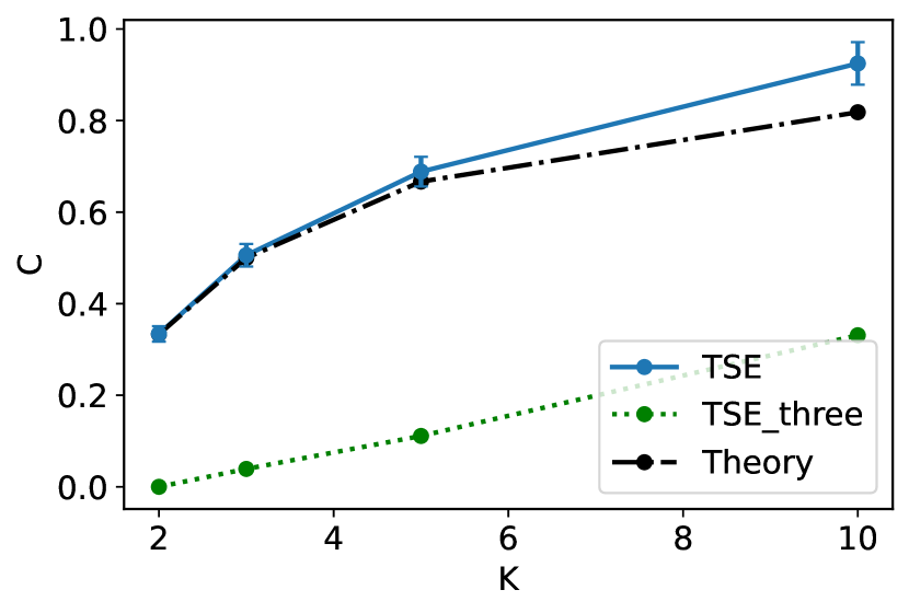
Figure 1: Comparison of $C_{\mathrm{opt}}$ ($=(K-1)/(K+1)$, Theory) and its estimated value using the TSE algorithm ($=\mathrm{R}_{H}(T)T^{\prime}$) with several different values of $K$. Here, the value of $T$ is set to $10^{5}K$ for each $K$. TSE_three indicates the simple regret when $|\hat{\mathcal{J}}^{*}|\geq 3$, with each bar representing two sigma of the corresponding plug-in variance.

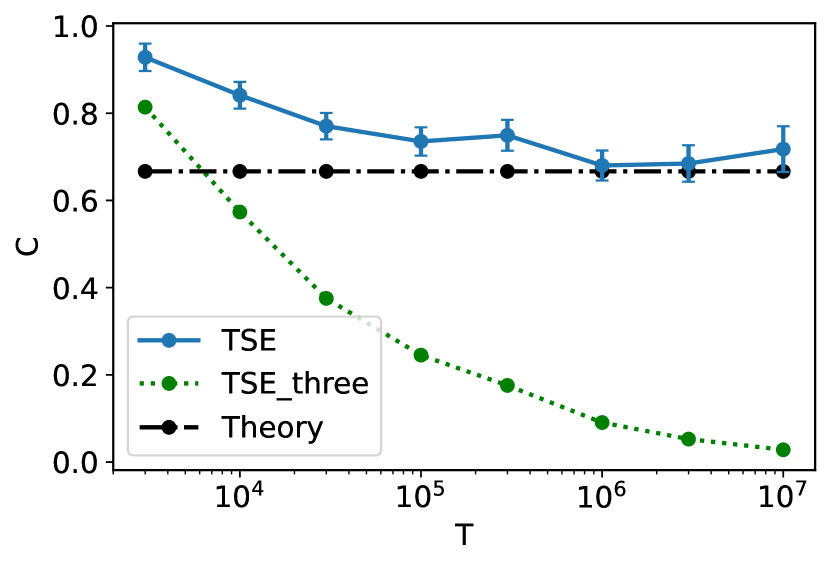
Figure 2: Comparison of $C_{\mathrm{opt}}$ (Theory) and its estimated value using the TSE algorithm ($=\mathrm{R}_{H}(T)T^{\prime}$) with several different values $T$. Here, $K$ is fixed to be $5$. The decreasing value of TSE_three implies that the probability of $|\hat{\mathcal{J}}^{*}|\geq 3$ is small if $T$ is large. Each bar represents two sigma of the corresponding plug-in variance.

We conducted a set of simulations to support our theoretical findings. We empirically tested the TSE algorithm (Algorithm 1) with the uniform prior (Example 2) and measured its simple regret with the aim of verifying the tightness of the upper bound of Theorem 1 with its leading order $C_{\mathrm{opt}}/T^{\prime}$. We set $q=0.5$ in the simulations.

To effectively sample small-gap cases, $\mathrm{R}_{H}(T)$ should be computed by a Monte Carlo rejection sampling of the prior $\bm{\mu}$ with an acceptance ratio

$$\max\left(\min\left(\frac{1}{2\Delta\sqrt{T}},1\right),0.01\right),$$ (59)

where $\Delta$ is the gap between the best arm and the second-best arm. Our simulation is implemented in the Python 3 programming language.

Figure 2 compares the performance of the TSE with the lower bound with several values of $K=\{2,3,5,10\}$. The results are averaged over $10^{5}$ runs. The TSE performs very closely to $C_{\mathrm{opt}}/T^{\prime}$, which implies the tightness of Theorem 1. The value $\mathrm{R}_{H}(T)$ is slightly larger than $C_{\mathrm{opt}}/T^{\prime}$ because the case of $|\hat{\mathcal{J}}^{*}|\geq 3$ is non-negligible unless $T$ is infinitely large. Furthermore, Figure 2 sets $K=5$ and compares several different values of $T$. Larger $T$ values increase the probability of $|\hat{\mathcal{J}}^{*}|=2$. Consequently, the simple regret of the TSE algorithm approaches the theoretical bound.

Note that this section does not aim to compare Algorithm 1 with existing algorithms. Although the TSE algorithm approaches the optimal bound by choosing a $q$ of $o(1)$, its practical performance has the capacity to improve. The value $q=0.5$ splits the two stages evenly and does not compromise the asymptotic rate by more than a factor of two, and we consider it to be a reasonable choice in practice.

5 Conclusion and Discussion

We have analyzed the Bayesian BAI in the context of the $K$-armed MAB problem, which concerns identifying the Bayes-optimal treatment allocation. We derived a lower bound of the Bayesian simple regret and introduced a simple algorithm that matches the lower bound under a mild regularity condition.

Our result is a counterpart of the Bayesian regret minimization (RM) of Lai, (1987) for the Bayesian simple regret minimization (SRM). Upon deriving a lower bound for Bayesian simple regret, we introduced a simple algorithm to match the lower bound under a mild regularity condition. Our results constitute the counterpart of the Bayesian RM of Lai, (1987) in the context of Bayesian SRM. Several particular differences between RM and SRM can be summarized:

• In RM, certain asymptotically optimal algorithms adopting a frequentist perspective are also optimal in terms of Bayesian RM and vice versa, whereas optimality in frequentist SRM remains inadequately characterized even though a seminal paper by Carpentier and Locatelli, (2016) exists.

• The leading term of Bayesian RM derives from the region of $\Delta>\sqrt{\frac{\log T}{T}}$, whereas the leading term of Bayesian SRM derives from $\Delta<\sqrt{\frac{\log T}{T}}$. This makes analyzing Bayesian simple regret challenging (Section 3.2). At the high level, Bayesian SRM involves quickly discarding clearly suboptimal arms and concentrating the rest of the samples on the competitive candidates of the best arm.

This paper has considered Bernoulli distributions, corresponding to observing a binary outcome for each treatment. Extending our results to other distributions, such as Gaussian distributions, would represent an interesting future research direction.

Appendix A Supplemental Example

This section shows an example in which the assumptions are violated.

Example 3.

(A prior that depends on $T$) Consider a two-armed case where the prior is

• With probability $0.5$, $\mu_{1}=T^{-1/2}$ and $\mu_{2}=0$.

• With probability $0.5$, $\mu_{1}=0$ and $\mu_{2}=T^{-1/2}$.

This prior violates the continuity assumption (Assumption 1) as well as it depends on $T$. It is not very difficult to show that the regret in this case is $\Theta(T^{-1/2})$, which is different from $O(T^{-1})$ regret that we have derived in the main paper.

Appendix B General Lemmas

Proposition 9.

(Stirling’s approximation) For any $n\in\mathbb{N}$, the following inequality holds:

$$\sqrt{2\pi}n^{n+\frac{1}{2}}e^{-n}e^{\frac{1}{12n+1}}<n!<\sqrt{2\pi}n^{n+\frac{1}{2}}e^{-n}e^{\frac{1}{12n}}.$$ (60)

By using $e^{1/n}\leq 1+2/n$ for $n\geq 2$, we have

$$\sqrt{2\pi}n^{n+\frac{1}{2}}e^{-n}<n!<\sqrt{2\pi}n^{n+\frac{1}{2}}e^{-n}\left(1+\frac{1}{6n}\right).$$ (61)

Lemma 10.

(Chernoff bound) Let $x_{1},x_{2},\dots,x_{n}$ be Bernoulli random variables with their common mean $\mu$. Let $\hat{\mu}_{n}=(1/n)\sum_{t=1}^{n}x_{t}$. Then,

$$\mathbb{P}\left[\hat{\mu}_{n}-\mu\geq\epsilon\right] \leq e^{-nd_{\mathrm{KL}}(\mu+\epsilon,\mu)},$$ (62)

$$\mathbb{P}\left[\hat{\mu}_{n}-\mu\leq-\epsilon\right] \leq e^{-nd_{\mathrm{KL}}(\mu-\epsilon,\mu)}.$$ (63)

Moreover, using the Pinsker’s inequality $d_{\mathrm{KL}}(p,q)\geq 2(p-q)^{2}$ and taking a union bound yields

$$\mathbb{P}\left[|\hat{\mu}_{n}-\mu|\geq\epsilon\right] \leq 2e^{-2n\epsilon^{2}}.$$ (64)

Appendix C Bounds on KL Divergence

Let $l\in[T^{-1/6},1-T^{-1/6}]$. Let $h(T)=o(T^{-1/6})$, and $T_{0}>0$ be such that $2h(T)<T^{-1/6}$ and $T^{-1/6}<1/2$ for all $T\geq T_{0}$. Let $u$ be such that $h(T)+l>u>l$. Let $m=(l+u)/2$ and $\Delta_{h}=(u-l)/2$.

Roughly speaking, Lemmas 11 and 12, which are below, state that

$$d_{\mathrm{KL}}(l,u)\approx 4d_{\mathrm{KL}}(l,m)\approx 4d_{\mathrm{KL}}(m,u)\approx\frac{(u-l)^{2}}{2l(1-l)}\approx\frac{(u-l)^{2}}{2m(1-m)}\approx\frac{(u-l)^{2}}{2u(1-u)}$$ (65)

when $\Delta_{h}$ is sufficiently small. We show the formal version of Eq. (65) in Lemma 13.

Lemma 11.

(Bound on the KL divergence around $l$)

For all $T\geq T_{0}$, the following inequality holds:

$$\left|d_{\mathrm{KL}}(l,u)-\frac{(u-l)^{2}}{2l(1-l)}\right|\leq C_{\mathrm{KL}}(h(T))^{3}T^{1/3},$$ (66)

Proof.

Proof of Lemma 11 Letting $\eta=\max(\frac{u-l}{l},\frac{1-l}{1-u})\leq 4h(T)T^{1/6}$, we have

$$d_{\mathrm{KL}}(l,u) :=\int_{x=0}^{u-l}\frac{d(d_{\mathrm{KL}}(l,l+x))}{dx}dx$$ (67)

$$=\int_{x=0}^{u-l}\frac{x}{(l+x)(1-l-x)}dx$$ (68)

$$\leq(1+2\eta)\int_{x=0}^{u-l}\frac{x}{l(1-l)}dx$$ (69)

$$=(1+2\eta)\frac{(u-l)^{2}}{2l(1-l)}$$ (70)

$$=\frac{(u-l)^{2}}{2l(1-l)}+2\eta\times\frac{(u-l)^{2}}{2l(1-l)}=\frac{(u-l)^{2}}{2l(1-l)}+2\eta\times\left((h(T))^{2}T^{1/6}\right)$$ (71)

$$\leq\frac{(u-l)^{2}}{2l(1-l)}+8\left((h(T))^{3}T^{1/3}\right).$$ (72)

Another inequality $\frac{(u-l)^{2}}{2l(1-l)}-8\left((h(T))^{3}T^{1/3}\right)\leq d_{\mathrm{KL}}(l,u)$ is derived in the same manner. ∎

Lemma 12.

For all $T\geq T_{0}$, the following inequalities hold:

$$|d_{\mathrm{KL}}(m,u)-d_{\mathrm{KL}}(l,m)| \leq C_{\mathrm{KL}}(h(T))^{3}T^{1/3}$$ (73)

$$|d_{\mathrm{KL}}(m,u)-d_{\mathrm{KL}}(u,m)| \leq C_{\mathrm{KL}}(h(T))^{3}T^{1/6},$$ (74)

for some universal constant $C_{\mathrm{KL}}>0$.

Proof.

Proof of Lemma 12

$$|d_{\mathrm{KL}}(m,u)-d_{\mathrm{KL}}(l,m)| =\left|\int_{x=l}^{m}\frac{d(d_{\mathrm{KL}}(x,x+\Delta_{h}))}{dx}dx\right|$$ (75)

$$\leq\Delta_{h}\max_{x\in[m,m+\Delta_{h}]}\left|\frac{d(d_{\mathrm{KL}}(x,x+\Delta_{h}))}{dx}\right|.$$ (76)

We have

$$\frac{d}{dx}d_{\mathrm{KL}}(x,x+\Delta_{h}) =\frac{d}{dx}\left(x\log\left(\frac{x}{x+\Delta_{h}}\right)+(1-x)\log\left(\frac{1-x}{1-x-\Delta_{h}}\right)\right)$$ (77)

$$=\left(\log\left(\frac{x}{x+\Delta_{h}}\right)-\log\left(\frac{1-x}{1-x-\Delta_{h}}\right)\right)+\left(\frac{\Delta_{h}}{x+\Delta_{h}}+\frac{\Delta_{h}}{1-x-\Delta_{h}}\right)$$ (78)

$$=\log\left(1-\frac{\Delta_{h}}{(x+\Delta_{h})(1-x)}\right)+\frac{\Delta_{h}}{(x+\Delta_{h})(1-x-\Delta_{h})}.$$ (79)

By using $|\frac{\Delta_{h}}{(x+\Delta_{h})(1-x)}|<1/2$ and $-y-y^{2}\leq\log(1-y)\leq-y$ for $y\in[0,1/2]$, we have

$$\left|\frac{d}{dx}d_{\mathrm{KL}}(x,x+\Delta_{h})\right| \leq\left|-\frac{\Delta_{h}}{(x+\Delta_{h})(1-x)}+\frac{\Delta_{h}}{(x+\Delta_{h})(1-x-\Delta_{h})}\right|$$

$$\qquad\qquad+\left|-\left(\frac{\Delta_{h}}{(x+\Delta_{h})(1-x)}\right)^{2}\right|$$

$$=\frac{\Delta_{h}^{2}}{(x+\Delta_{h})(1-x)(1-x-\Delta)}+\left(\frac{\Delta_{h}}{(x+\Delta_{h})(1-x)}\right)^{2}$$

which, by using $\Delta_{h}<h(T)/2=o(T^{-1/6})$ and $x,1-x>T^{-1/6}$, can be easily bounded by $C{\Delta_{h}^{2}}T^{1/3}$ for some $C>0$, which is Eq. (73).

We next derive Eq. (74).

$$d_{\mathrm{KL}}(m,u)-d_{\mathrm{KL}}(m,l) =\int_{x=0}^{\Delta_{h}}\frac{x}{(m+x)(1-m-x)}dx-\int_{x=0}^{\Delta_{h}}\frac{x}{(m-x)(1-m+x)}dx$$ (80)

$$=\int_{x=0}^{\Delta_{h}}\frac{2x^{2}(2m-1)}{(m^{2}-x^{2})((1-x)^{2}-m^{2})}dx$$ (81)

and thus

$$|d_{\mathrm{KL}}(m,u)-d_{\mathrm{KL}}(m,l)| \leq\Delta_{h}\times\max\left|\frac{2\Delta_{h}^{2}(2m-1)}{(m^{2}-x^{2})((1-x)^{2}-m^{2})}\right|$$ (82)

$$=C\Delta_{h}^{3}T^{1/6}$$ (83)

for some $C>0$, which is Eq. (74). ∎

Lemma 13.

(Bound on the KL divergence) Let $h(T)=\sqrt{C_{h}\log T/T}$ for some constant $C_{h}>0$. Then, there exist $C_{a}>0,T_{0}$ for all $T\geq T_{0}$,

$$\frac{(u-l)^{2}}{2m(1-m)}-C_{a}T^{-1/6}(\log T)^{3}\leq d_{\mathrm{KL}}(l,u),d_{\mathrm{KL}}(u,l)\leq\frac{(u-l)^{2}}{2m(1-m)}+C_{a}T^{-1/6}(\log T)^{3}$$ (84)

and

$$\frac{(u-l)^{2}}{8m(1-m)}-C_{a}T^{-1/6}(\log T)^{3}\leq d_{\mathrm{KL}}(m,u),d_{\mathrm{KL}}(u,m),d_{\mathrm{KL}}(m,l),d_{\mathrm{KL}}(l,m)\leq\frac{(u-l)^{2}}{8m(1-m)}+C_{a}T^{-1/6}(\log T)^{3}.$$ (85)

The proof of Lemma 13 is straightforward from Lemmas 11 and 12.

Appendix D Lemmas for Upper Bound

D.1 Proof of Lemma 2

Proof.

Proof of Lemma 2 At the end of round $qT$, TSE draws each arm for $N_{i}(qT)=qT/K$ times. Eq. (16) is derived by using the union bound of the Hoeffding inequality (Eq. (64)) over $K$ arms. ∎

D.2 Proof of Lemma 3

Proof.

Proof of Lemma 3

$$\mathbb{E}_{\bm{\mu}\sim H}\left[\mathbb{E}_{\bm{\mu}}[\bm{1}[\mathcal{S},|\hat{\mathcal{J}}^{*}|\geq 3]\Delta_{J(T)}]\right]$$ (86)

$$\leq 4B_{\mathrm{conf}}\sum_{i,j,k}\int\bm{1}\left[\mu_{i}\geq\mu_{k}-4B_{\mathrm{conf}},\mu_{j}\geq\mu_{k}-4B_{\mathrm{conf}}\right]dH(\bm{\mu})$$ (87)

$$=4B_{\mathrm{conf}}\sum_{i,j,k}\int\bm{1}\left[|\mu_{i}-\mu_{k}|\leq 4B_{\mathrm{conf}},|\mu_{j}-\mu_{k}|\leq 4B_{\mathrm{conf}}\right]h_{ij}(\mu_{i},\mu_{j}|\bm{\mu}_{\setminus ij})d\mu_{i}d\mu_{j}dH_{\setminus ij}(\bm{\mu}_{\setminus ij}).$$ (88)

By choosing $\epsilon=1$ in Eq. (4), for any $T$ such that $4B_{\mathrm{conf}}(T)\leq\delta(\epsilon)=\delta(1)$, for each $\bm{\mu}_{\setminus ij}$, we have

$$\int\bm{1}\left[|\mu_{i}-\mu_{k}|\leq 4B_{\mathrm{conf}},|\mu_{j}-\mu_{k}|\leq 4B_{\mathrm{conf}}\right]d\mu_{i}d\mu_{j}\leq\int\bm{1}\left[\sqrt{(\mu_{i}-\mu_{k})^{2}+(\mu_{j}-\mu_{k})^{2}}\leq\sqrt{2}\delta(1)\right]d\mu_{i}d\mu_{j}.$$ (89)

By using this, we have

$$4B_{\mathrm{conf}}\int\bm{1}\left[|\mu_{i}-\mu_{k}|\leq 4B_{\mathrm{conf}},|\mu_{j}-\mu_{k}|\leq 4B_{\mathrm{conf}}\right]h(\mu_{i},\mu_{j}|\bm{\mu}_{\setminus ij})d\mu_{i}d\mu_{j}dH_{\setminus ij}(\bm{\mu}_{\setminus ij})$$ (90)

$$\leq 4B_{\mathrm{conf}}\int\bm{1}\left[|\mu_{i}-\mu_{k}|\leq 4B_{\mathrm{conf}},|\mu_{j}-\mu_{k}|\leq 4B_{\mathrm{conf}}\right]\left(h(\mu_{k},\mu_{k}|\bm{\mu}_{\setminus ij})+1\right)d\mu_{i}d\mu_{j}dH_{\setminus ij}(\bm{\mu}_{\setminus ij})$$ (91)

    (by uniform continuity and Eq. (89)) (92)

$$=O\left((B_{\mathrm{conf}})^{3}\right)=o\left(\frac{1}{T}\right).$$ (93)

∎

D.3 Lemmas on the main term

Let $m=(\mu_{i}+\mu_{j})/2$, $\Delta=\mu_{i}-\mu_{j}>0$, and $T^{\prime}_{h}=T^{\prime}/2$. Let $\hat{\mu}_{i,n}$ be the empirical mean of arm $i$ with the first $n$ samples.

Lemma 14.

(Tight Bayesian bound) The following inequality holds:

$$\int_{\mu_{j}}^{\min(\mu_{j}+2B_{\mathrm{conf}},1-T^{-1/6})}(\mu_{i}-\mu_{j})\mathbb{P}_{\bm{\mu}}[\hat{\mu}_{i,T^{\prime}_{h}}\leq\hat{\mu}_{j,T^{\prime}_{h}},\mathcal{S}]d\mu_{i}\leq(1+o(1))\frac{m(1-m)}{T^{\prime}}.$$ (94)

Remark 4.

(Lemma 14 is tighter than the Chernoff bound) In the proof of Lemma 14, we carefully use the change-of-measure argument to derive a tight bound. Alternatively, we may use the concentration inequality (Chernoff bound, Lemma 10) in bounding the regret, which yields

$$\mathbb{P}[\hat{\mu}_{i}(T)\leq\hat{\mu}_{j}(T)]\leq\mathbb{P}[\hat{\mu}_{i}(T)\leq m]+\mathbb{P}[\hat{\mu}_{j}(T)\geq m]\approx 2e^{-T^{\prime}_{h}d_{\mathrm{KL}}(\mu_{j},m)}$$ (95)

which, integrated over the prior, is four times larger than Lemma 14.

Lemma 15.

(Tight frequentist bound) Let $\mu_{\setminus ij}^{*}<\mu_{j}<\mu_{i}<\min(\mu_{j}+2B_{\mathrm{conf}},1-T^{-1/6})$. Then,

$$\mathbb{P}_{\bm{\mu}}[\hat{\mu}_{i,T^{\prime}_{h}}\leq\hat{\mu}_{j,T^{\prime}_{h}},\mathcal{S}]=(1+o(1))\sqrt{\frac{T^{\prime}}{8\pi m(1-m)}}\int_{s_{2}=0}^{\infty}e^{-\frac{T^{\prime}}{8m(1-m)}\left(\Delta^{2}+2s_{2}\Delta+s_{2}^{2}\right)}ds_{2},$$ (96)

where the $o(1)$ term does not depend on $\mu_{i},\mu_{j}$.

Particular care is required in Lemma 15 because a high-probability bound on the KL divergence is not tight (c.f., Section 3.2); we can upper-bound a simple regret based on a high-probability bound on the KL divergence, simplifying the analysis of Lemma 15. However, such a high-probability bound compromises the leading constant. In the following proof, we use Proposition 9, Lemma 13, and manual calculation on the number of combinations because these operations are tight concerning the leading constant.

Proof.

Proof of Lemma 15

Let

$$\bm{\lambda}:=(\mu_{1},\mu_{2},\dots,\mu_{i-1},\underbrace{m}_{\text{$i$-th element}},\mu_{i+1},\dots,\mu_{j-1},\underbrace{m}_{\text{$j$-th element}},\mu_{j+1},\dots,\mu_{K})$$

be the set of parameters where $(\mu_{i},\mu_{j})$ is replaced by $(m,m)$. Let $\hat{\mu}_{i,n}$ be the empirical mean of arm $i$ with $n$ samples.

Under $\mu_{j}+2B_{\mathrm{conf}}>\mu_{i}>\mu_{j}>\mu_{\setminus ij}^{*}$, we have

$$\{\hat{\mu}_{i,T^{\prime}_{h}}\leq\hat{\mu}_{j,T^{\prime}_{h}},\mathcal{S}\}$$ (97)

$$=\{T^{\prime}_{h}\,\hat{\mu}_{i,T^{\prime}_{h}}\leq T^{\prime}_{h}\,\hat{\mu}_{j,T^{\prime}_{h}},\mathcal{S}\}$$ (98)

$$=(T^{\prime}_{h}\,\hat{\mu}_{i,T^{\prime}_{h}},T^{\prime}_{h}\,\hat{\mu}_{j,T^{\prime}_{h}})\subseteq\{(T_{1},T_{2})\in\mathbb{N}^{2}:-4TB_{\mathrm{conf}}\leq T_{1}-T^{\prime}_{h}m\leq T_{2}-T^{\prime}_{h}m\leq 4TB_{\mathrm{conf}}\}$$ (99)

$$\ \ \ :=\mathcal{S}_{i,j}$$ (100)

Let $(D_{1},D_{2})=(T_{1}-T^{\prime}_{h}m,T_{2}-T^{\prime}_{h}m)$. We have

$$\mathbb{P}_{\bm{\mu}}[\hat{\mu}_{i,T^{\prime}_{h}}\leq\hat{\mu}_{j,T^{\prime}_{h}},\mathcal{S}]$$ (101)

$$=\sum_{(T_{1},T_{2})\in\mathcal{S}_{i,j}}\mathbb{P}_{\bm{\mu}}\left[T^{\prime}_{h}\,\hat{\mu}_{i,T^{\prime}_{h}}=T_{1},\,T^{\prime}_{h}\,\hat{\mu}_{j,T^{\prime}_{h}}=T_{2}\right]$$ (102)

$$=\sum_{(T_{1},T_{2})\in\mathcal{S}_{i,j}}e^{(D_{1}+T^{\prime}_{h}m)\log\left(\frac{\mu_{i}}{m}\right)+(T^{\prime}_{h}(1-m)-D_{1})\log\left(\frac{1-\mu_{i}}{1-m}\right)+(D_{2}+T^{\prime}_{h}m)\log\left(\frac{\mu_{j}}{m}\right)+(T^{\prime}_{h}(1-m)-D_{2})\log\left(\frac{1-\mu_{j}}{1-m}\right)}$$ (103)

$$\ \ \ \ \ \ \ \ \ \ \times\mathbb{P}_{\bm{\lambda}}\left[T^{\prime}_{h}\,\hat{\mu}_{i,T^{\prime}_{h}}=T_{1},T^{\prime}_{h}\,\hat{\mu}_{j,T^{\prime}_{h}}=T_{2}\right]$$ (104)

       (change of measure) (105)

$$=\sum_{(T_{1},T_{2})\in\mathcal{S}_{i,j}}e^{-T^{\prime}_{h}\left(d_{\mathrm{KL}}(m,\mu_{i})+d_{\mathrm{KL}}(m,\mu_{j})\right)+\left(D_{1}\log\left(\frac{\mu_{i}}{m}\right)-D_{1}\log\left(\frac{1-\mu_{i}}{1-m}\right)+D_{2}\log\left(\frac{\mu_{j}}{m}\right)-D_{2}\log\left(\frac{1-\mu_{j}}{1-m}\right)\right)}$$ (106)

$$\ \ \ \ \ \ \ \ \ \ \times\mathbb{P}_{\bm{\lambda}}\left[T^{\prime}_{h}\,\hat{\mu}_{i,T^{\prime}_{h}}=T_{1},\,T^{\prime}_{h}\,\hat{\mu}_{j,T^{\prime}_{h}}=T_{2}\right]$$ (107)

$$=\sum_{(T_{1},T_{2})\in\mathcal{S}_{i,j}}e^{-(1-o(1))\left(\frac{T^{\prime}\Delta^{2}}{8m(1-m)}\right)+\left(D_{1}\log\left(\frac{\mu_{i}}{m}\right)-D_{1}\log\left(\frac{1-\mu_{i}}{1-m}\right)+D_{2}\log\left(\frac{\mu_{j}}{m}\right)-D_{2}\log\left(\frac{1-\mu_{j}}{1-m}\right)\right)}$$ (108)

$$\ \ \ \ \ \ \ \ \ \ \times\mathbb{P}_{\bm{\lambda}}\left[T^{\prime}_{h}\,\hat{\mu}_{i,T^{\prime}_{h}}=T_{1},\,T^{\prime}_{h}\,\hat{\mu}_{j,T^{\prime}_{h}}=T_{2}\right]$$ (109)

       (By Lemma 13) (110)

$$=\sum_{(T_{1},T_{2})\in\mathcal{S}_{i,j}}e^{-(1-o(1))\left(\frac{T^{\prime}\Delta^{2}}{8m(1-m)}+D_{1}\frac{\Delta}{2m(1-m)}-D_{2}\frac{\Delta}{2m(1-m)}\right)}$$ (111)

$$\ \ \ \ \ \ \ \ \ \ \times\mathbb{P}_{\bm{\lambda}}\left[T^{\prime}_{h}\,\hat{\mu}_{i,T^{\prime}_{h}}=T_{1},\,T^{\prime}_{h}\,\hat{\mu}_{j,T^{\prime}_{h}}=T_{2}\right]$$ (112)

       (By $$|\log(1+x)-x|=O(x^{2}) \left|\frac{\mu_{i}(1-m)}{m(1-\mu_{i})}-1-\frac{\Delta}{2m(1-m)}\right|=o(\Delta)$$ and ) (113)

$$=\sum_{(T_{1},T_{2})\in\mathcal{S}_{i,j}}e^{-(1-o(1))\left(\frac{T^{\prime}\Delta^{2}}{8m(1-m)}+D_{1}\frac{\Delta}{2m(1-m)}-D_{2}\frac{\Delta}{2m(1-m)}\right)}$$ (114)

$$\ \ \ \ \ \ \ \ \ \ \times\frac{T^{\prime}_{h}!}{T_{1}!(T^{\prime}_{h}-T_{1})!}m^{T_{1}}(1-m)^{T^{\prime}_{h}-T_{1}}\frac{T^{\prime}_{h}!}{T_{2}!(T^{\prime}_{h}-T_{2})!}m^{T_{2}}(1-m)^{T^{\prime}_{h}-T_{2}}$$ (115)

          (by number of combinations) (116)

$$=\sum_{(T_{1},T_{2})\in\mathcal{S}_{i,j}}e^{-(1-o(1))\left(\frac{T^{\prime}\Delta^{2}}{8m(1-m)}+D_{1}\frac{\Delta}{2m(1-m)}-D_{2}\frac{\Delta}{2m(1-m)}\right)}$$ (117)

$$\ \ \ \ \ \ \ \ \ \ \times\frac{1}{\sqrt{2\pi}}e^{(1+o(1))\left((T^{\prime}_{h}+\frac{1}{2})\log(T^{\prime}_{h})-(T_{1}+\frac{1}{2})\log(T_{1})-(T^{\prime}_{h}-T_{1}+\frac{1}{2})\log(T^{\prime}_{h}-T_{1})+T_{1}\log(m)+(T^{\prime}_{h}-T_{1})\log(1-m)\right)}$$ (118)

$$\ \ \ \ \ \ \ \ \ \ \times\frac{1}{\sqrt{2\pi}}e^{(1+o(1))\left((T^{\prime}_{h}+\frac{1}{2})\log(T^{\prime}_{h})-(T_{2}+\frac{1}{2})\log(T_{2})-(T^{\prime}_{h}-T_{2}+\frac{1}{2})\log(T^{\prime}_{h}-T_{2})+T_{2}\log(m)+(T^{\prime}_{h}-T_{2})\log(1-m)\right)}.$$ (119)

          (by Proposition 9) (121)

Here, letting $(t_{1},t_{2})=(T_{1}/T^{\prime}_{h},T_{2}/T^{\prime}_{h}$), we have

$$e^{(T^{\prime}_{h}+\frac{1}{2})\log(T^{\prime}_{h})-(T_{1}+\frac{1}{2})\log(T_{1})-(T^{\prime}_{h}-T_{1}+\frac{1}{2})\log(T^{\prime}_{h}-T_{1})+T_{1}\log(m)+(T^{\prime}_{h}-T_{1})\log(1-m)}$$ (122)

$$=\sqrt{\frac{T^{\prime}_{h}}{T_{1}(T^{\prime}_{h}-T_{1})}}e^{(1+o(1))\left(T^{\prime}_{h}\log(T^{\prime}_{h})-T_{1}\log(T_{1})-(T^{\prime}_{h}-T_{1})\log(T^{\prime}_{h}-T_{1})+T_{1}\log(m)+(T^{\prime}_{h}-T_{1})\log(1-m)\right)}$$ (123)

$$=\sqrt{\frac{2}{m(1-m)T^{\prime}}}e^{(1+o(1))\left(T^{\prime}_{h}\log(T^{\prime}_{h})-T_{1}\log(T_{1})-(T^{\prime}_{h}-T_{1})\log(T^{\prime}_{h}-T_{1})+T_{1}\log(m)+(T^{\prime}_{h}-T_{1})\log(1-m)\right)}$$ (124)

          (by $$T_{1},T_{2}=mT^{\prime}_{h}+O(TB_{\mathrm{conf}})$$)) (125)

$$=\sqrt{\frac{2}{m(1-m)T^{\prime}}}e^{(1+o(1))T^{\prime}_{h}\left(-t_{1}\log(t_{1})-(1-t_{1})\log(1-t_{1})+t_{1}\log(m)+(1-t_{1})\log(1-m)\right)}$$ (126)

$$=\sqrt{\frac{2}{m(1-m)T^{\prime}}}e^{-(1-o(1))T^{\prime}_{h}d_{\mathrm{KL}}(m,t_{1})}$$ (127)

and thus, by letting $(d_{1},d_{2})=(D_{1}/T^{\prime}_{h},D_{2}/T^{\prime}_{h})$, we have

Eq. (LABEL:ineq_newfreq_temp) (128)

$$=\frac{1}{2\pi}\frac{2}{m(1-m)T^{\prime}}\sum_{(T_{1},T_{2})\in\mathcal{S}_{i,j}}e^{-(1-o(1))\left(\frac{T^{\prime}\Delta^{2}}{8m(1-m)}+D_{1}\frac{\Delta}{2m(1-m)}-D_{2}\frac{\Delta}{2m(1-m)}+T^{\prime}_{h}d_{\mathrm{KL}}(m,t_{1})+T^{\prime}_{h}d_{\mathrm{KL}}(m,t_{2})\right)}$$ (129)

          (by Eq. (127)) (130)

$$=\frac{1}{\pi m(1-m)T^{\prime}}\sum_{(T_{1},T_{2})\in\mathcal{S}_{i,j}}e^{-(1-o(1))\left(\frac{T^{\prime}\Delta^{2}}{8m(1-m)}+D_{1}\frac{\Delta}{2m(1-m)}-D_{2}\frac{\Delta}{2m(1-m)}+T^{\prime}_{h}d_{\mathrm{KL}}(m,t_{1})+T^{\prime}_{h}d_{\mathrm{KL}}(m,t_{2})\right)}$$ (131)

$$=\frac{1}{\pi m(1-m)T^{\prime}}\sum_{(T_{1},T_{2})\in\mathcal{S}_{i,j}}e^{-(1-o(1))\frac{T^{\prime}}{8m(1-m)}\left(\Delta^{2}+2d_{1}\Delta-2d_{2}\Delta+2d_{1}^{2}+2d_{2}^{2}\right)}$$ (132)

       (By Lemma 13) (133)

$$=\frac{1+o(1)}{\pi m(1-m)T^{\prime}}\sum_{(T_{1},T_{2})\in\mathcal{S}_{i,j}}e^{-\frac{T^{\prime}}{8m(1-m)}\left(\Delta^{2}+2d_{1}\Delta-2d_{2}\Delta+2d_{1}^{2}+2d_{2}^{2}\right)}$$ (134)

$$=\frac{(1+o(1))T^{\prime}}{4\pi m(1-m)}\int_{t_{1}=-\infty}^{\infty}\int_{t_{2}=t_{1}}^{\infty}e^{-\frac{T^{\prime}}{8m(1-m)}\left(\Delta^{2}+2d_{1}\Delta-2d_{2}\Delta+2d_{1}^{2}+2d_{2}^{2}\right)}d(d_{1})d(d_{2})$$ (135)

          (by $$dD_{1}=\frac{T^{\prime}}{2}d(d_{1}),dD_{2}=\frac{T^{\prime}}{2}d(d_{2})$$) (136)

$$=\frac{(1+o(1))T^{\prime}}{8\pi m(1-m)}\int_{s_{1}=-\infty}^{\infty}\int_{s_{2}=0}^{\infty}e^{-\frac{T^{\prime}}{8m(1-m)}\left(\Delta^{2}+2s_{2}\Delta+s_{1}^{2}+s_{2}^{2}\right)}ds_{1}ds_{2}$$ (137)

          (by letting $$s_{1},s_{2}=(d_{1}+d_{2}),(d_{2}-d_{1}) ds_{1}ds_{2}=2d(d_{1})d(d_{2})$$ and ) (138)

$$=\sqrt{\frac{8m(1-m)}{\pi T^{\prime}}}\frac{(1+o(1))T^{\prime}}{8m(1-m)}\int_{s_{2}=0}^{\infty}e^{-\frac{T^{\prime}}{8m(1-m)}\left(\Delta^{2}+2s_{2}\Delta+s_{2}^{2}\right)}ds_{2}.$$ (139)

          (by $$\int_{-\infty}^{\infty}\exp(-x^{2})dx=\sqrt{\pi}$$) (140)

This concludes the proof. Note that the $o(1)$ term is derived by applying Lemma 13, where the term $C_{a}T^{-1/6}(\log T)^{3}$ does not depend on $\mu_{i},\mu_{j}$. ∎

Proof.

Proof of Lemma 14 An integration of Lemma 15 over $\Delta=\mu_{i}-\mu_{j}$ from $0$ to a sufficiently large value is

$$(1+o(1))\sqrt{\frac{T^{\prime}}{8\pi m(1-m)}}\int_{\mu_{j}}^{2B_{\mathrm{conf}}}\Delta\int_{s_{2}=0}^{\infty}e^{-\frac{T^{\prime}}{8m(1-m)}(\Delta+s_{2})^{2}}ds_{2}d\Delta$$ (141)

$$\leq(1+o(1))\sqrt{\frac{T^{\prime}}{8\pi m(1-m)}}\int_{\Delta=0}^{\infty}\Delta\int_{s_{2}=0}^{\infty}e^{-\frac{T^{\prime}}{8m(1-m)}(\Delta+s_{2})^{2}}ds_{2}d\Delta$$ (142)

$$=(1+o(1))\sqrt{\frac{T^{\prime}}{8\pi m(1-m)}}\int_{s_{2}=0}^{\infty}\int_{\Delta=0}^{\infty}\Delta e^{-\frac{T^{\prime}}{8m(1-m)}(\Delta+s_{2})^{2}}d\Delta ds_{2}$$ (143)

$$=\frac{1+o(1)}{2}\sqrt{\frac{T^{\prime}}{8\pi m(1-m)}}\int_{s_{2}=0}^{\infty}\int_{\Delta=0}^{\infty}(\Delta+s_{2})e^{-\frac{T^{\prime}}{8m(1-m)}(\Delta+s_{2})^{2}}d\Delta ds_{2}$$ (144)

          (by $$\int_{0}^{\infty}\int_{0}^{\infty}xe^{-(x+y)^{2}}dxdy=\frac{1}{2}\int_{0}^{\infty}\int_{0}^{\infty}xe^{-(x+y)^{2}}dxdy+\frac{1}{2}\int_{0}^{\infty}\int_{0}^{\infty}ye^{-(x+y)^{2}}dxdy$$) (145)

$$=\frac{1+o(1)}{2}\sqrt{\frac{T^{\prime}}{8\pi m(1-m)}}\int_{s_{2}=0}^{\infty}\left[-\frac{4m(1-m)}{T^{\prime}}e^{-\frac{T^{\prime}}{8m(1-m)}(\Delta+s_{2})^{2}}\right]_{\Delta=0}^{\infty}ds_{2}$$ (146)

$$=(1+o(1))\sqrt{\frac{m(1-m)}{2\pi T^{\prime}}}\int_{s_{2}=0}^{\infty}e^{-\frac{T^{\prime}}{8m(1-m)}s_{2}^{2}}ds_{2}$$ (147)

$$=(1+o(1))\frac{m(1-m)}{T^{\prime}}.$$ (148)

          (by $$\int_{0}^{\infty}\exp(-x^{2})dx=\sqrt{\pi}/2$$) (149)

∎

D.4 Proof of Lemma 4

Proof.

Proof of Lemma 4 Event $\mathcal{S}$ implies that $i^{*}\in\hat{\mathcal{J}}^{*}$. Under $\hat{\mathcal{J}}^{*}=\{i,j\}$, we have $N_{i}(T)=N_{j}(T)=T^{\prime}_{h}$.

$$\mathbb{E}_{\bm{\mu}\sim H}\left[\mathbb{E}_{\bm{\mu}}[\bm{1}[\mathcal{S},|\hat{\mathcal{J}}^{*}|=2]\Delta_{J(T)}]\right]$$ (150)

$$\leq\sum_{i,j}\mathbb{E}_{\bm{\mu}\sim H}\left[\bm{1}[\mathcal{S},\mu_{i}>\mu_{j}>\mu_{\setminus ij}^{*}]\mathbb{E}_{\bm{\mu}}[\bm{1}[\mathcal{S},\hat{\mathcal{J}}^{*}=\{i,j\}]\Delta_{J(T)}]\right]$$ (151)

$$\leq\sum_{i,j}\mathbb{E}_{\bm{\mu}\sim H}\left[\bm{1}[\mu_{j}+2B_{\mathrm{conf}}>\mu_{i}>\mu_{j}>\mu_{\setminus ij}^{*},]\mathbb{E}_{\bm{\mu}}[\bm{1}[\mathcal{S},\hat{\mathcal{J}}^{*}=\{i,j\}]\Delta_{J(T)}]\right]$$ (152)

$$=\sum_{i,j}\mathbb{E}_{\bm{\mu}\sim H}\left[\bm{1}[\mu_{j}+2B_{\mathrm{conf}}>\mu_{i}>\mu_{j}>\mu_{\setminus ij}^{*}](\mu_{i}-\mu_{j})\mathbb{P}_{\bm{\mu}}[\hat{\mu}_{i,T^{\prime}_{h}}\leq\hat{\mu}_{j,T^{\prime}_{h}},\mathcal{S}]\right]$$ (153)

$$=\sum_{i,j}\mathbb{E}_{\bm{\mu}\sim H}\left[\bm{1}[\mu_{j}+2B_{\mathrm{conf}}>\mu_{i}>\mu_{j}>\mu_{\setminus ij}^{*},1-T^{-1/6}>\mu_{i}](\mu_{i}-\mu_{j})\mathbb{P}_{\bm{\mu}}[\hat{\mu}_{i,T^{\prime}_{h}}\leq\hat{\mu}_{j,T^{\prime}_{h}},\mathcal{S}]\right]$$ (154)

$$\ \ \ \ \ +\sum_{i,j}2B_{\mathrm{conf}}O\left(\mathbb{P}_{\bm{\mu}\sim H}[\mu_{i}>1-T^{-1/6},|\mu_{i}-\mu_{j}|\leq 2B_{\mathrm{conf}}]\right).$$ (155)

$$=\sum_{i,j}\mathbb{E}_{\bm{\mu}\sim H}\left[\bm{1}[\mu_{j}+2B_{\mathrm{conf}}>\mu_{i}>\mu_{j}>\mu_{\setminus ij}^{*},1-T^{-1/6}>\mu_{i}](\mu_{i}-\mu_{j})\mathbb{P}_{\bm{\mu}}[\hat{\mu}_{i,T^{\prime}_{h}}\leq\hat{\mu}_{j,T^{\prime}_{h}},\mathcal{S}]\right]+o\left(\frac{1}{T}\right)$$ (156)

     (by uniform continuity) (157)

$$\leq\sum_{i}\mathbb{E}_{\bm{\mu}\sim H}\left[\bm{1}[\mu_{\setminus i}^{*}+2B_{\mathrm{conf}}>\mu_{i}>\mu_{\setminus i}^{*},1-T^{-1/6}>\mu_{i}](\mu_{i}-\mu_{\setminus i}^{*})\mathbb{P}_{\bm{\mu}}[\hat{\mu}_{i,T^{\prime}_{h}}\leq\hat{\mu}_{j,T^{\prime}_{h}},\mathcal{S}]\right]+o\left(\frac{1}{T}\right).$$ (158)

Here, the first term of Eq. (158) is bounded as:

$$\mathbb{E}_{\bm{\mu}\sim H}\left[\bm{1}[\mu_{\setminus i}^{*}+2B_{\mathrm{conf}}>\mu_{i}>\mu_{\setminus i}^{*},1-T^{-1/6}>\mu_{i}](\mu_{i}-\mu_{\setminus i}^{*})\mathbb{P}_{\bm{\mu}}[\hat{\mu}_{i,T^{\prime}_{h}}\leq\hat{\mu}_{j,T^{\prime}_{h}},\mathcal{S}]\right]$$ (159)

$$\leq\int_{[0,1]^{K-1}}\int_{\mu_{i}=\mu_{\setminus i}^{*}}^{\min(\mu_{\setminus i}^{*}+2B_{\mathrm{conf}},1-T^{-1/6})}(\mu_{i}-\mu_{\setminus i}^{*})\mathbb{P}_{\bm{\mu}}[\hat{\mu}_{i,T^{\prime}_{h}}\leq\hat{\mu}_{j,T^{\prime}_{h}},\mathcal{S}]h_{i}(\mu_{i}|\bm{\mu}_{\setminus i})d\mu_{i}dH_{\setminus i}(\bm{\mu}_{\setminus i})$$ (160)

$$\leq(1+o(1))\int_{[0,1]^{K-1}}h_{i}(\mu_{\setminus i}^{*}|\bm{\mu}_{\setminus i})\int_{\mu_{i}=\mu_{\setminus i}^{*}}^{\min(\mu_{\setminus i}^{*}+2B_{\mathrm{conf}},1-T^{-1/6})}(\mu_{i}-\mu_{\setminus i}^{*})\mathbb{P}_{\bm{\mu}}[\hat{\mu}_{i,T^{\prime}_{h}}\leq\hat{\mu}_{j,T^{\prime}_{h}},\mathcal{S}]d\mu_{i}dH_{\setminus i}(\bm{\mu}_{\setminus i})$$ (161)

   (by uniform continuity) (162)

$$\leq(1+o(1))\int_{[0,1]^{K-1}}h_{i}(\mu_{\setminus i}^{*}|\bm{\mu}_{\setminus i})\frac{\mu_{\setminus i}^{*}(1-\mu_{\setminus i}^{*})}{T^{\prime}}dH_{\setminus i}(\bm{\mu}_{\setminus i}),$$ (163)

   (by the union bound of Lemma 14 over all $$j\neq i$$) (164)

which completes the proof. ∎

Appendix E Lemmas for Lower Bound

E.1 Lower bound on the error

Proposition 16.

(Lemma 1 of Kaufmann et al., (2016)) Let $\bm{\mu},\bm{\nu}\in[0,1]^{K}$ be two sets of model parameters. Then, for any event $\mathcal{E}$, the following inequality holds:

$$\sum_{i\in[K]}\mathbb{E}_{\bm{\nu}}[N_{i}(T)]d_{\mathrm{KL}}(\nu_{i},\mu_{i})\geq d_{\mathrm{KL}}(\mathbb{P}_{\bm{\nu}}(\mathcal{E}),\mathbb{P}_{\bm{\mu}}(\mathcal{E})).$$ (165)

Moreover,

$$\forall_{x\in[0,1]}d_{\mathrm{KL}}(x,1-x)\geq\log\frac{1}{2.4x}.$$ (166)

Proposition 16 describes the hardness of identifying two different sets of parameters. By using this proposition, we derive Lemma 7.

Proof.

Proof of Lemma 7 We assume that Eq. (37) is false and derive a contradiction; that is, suppose that

$$\max(\mathbb{P}_{\bm{\mu}}[J(T)\neq i],\mathbb{P}_{\bm{\nu}}[J(T)\neq j])<\frac{1}{2.4}\exp\Big{(}-(1+\eta)Td_{\mathrm{KL}}(\mu_{j},\mu_{i})\Big{)}.$$

Let $p=\frac{1}{2.4}\exp\left(-(1+\eta)Td_{\mathrm{KL}}(\mu_{j},\mu_{i})\right)$. Then, Proposition 16 with $\mathcal{E}=\{J(T)\neq i\}$ yields

$$T\max\left(d_{\mathrm{KL}}(\mu_{j},\mu_{i}),d_{\mathrm{KL}}(\mu_{i},\mu_{j})\right) \geq\sum_{i\in[K]}\mathbb{E}_{\bm{\nu}}[N_{i}(T)]d_{\mathrm{KL}}(\nu_{i},\mu_{i})$$ (167)

$$\geq d_{\mathrm{KL}}(\mathbb{P}_{\bm{\nu}}[J(T)\neq i],\mathbb{P}_{\bm{\mu}}[J(T)\neq i])$$ (168)

    (by Proposition 16) (169)

$$\geq d_{\mathrm{KL}}(p,1-p)$$ (170)

    (by Eq. (37) is false) (171)

$$\geq\log\frac{1}{2.4p}$$ (172)

    (by Eq. (166)) (173)

$$\geq(1+\eta)Td_{\mathrm{KL}}(\mu_{j},\mu_{i})$$ (174)

$$\geq(1+\eta)(1-\eta^{\prime})T\max\left(d_{\mathrm{KL}}(\mu_{j},\mu_{i}),d_{\mathrm{KL}}(\mu_{i},\mu_{j})\right),$$ (175)

    (for some constant $$C>0 \eta^{\prime}=C\times B_{\mathrm{conf}}T^{1/3}$$ and by Lemma 12) (176)

which contradicts for some $C_{2}>0$ and $\eta=C_{2}\times B_{\mathrm{conf}}T^{1/3}$ such that $(1+\eta)(1-\eta^{\prime})>1$, and thus Eq. (37) holds. ∎

E.2 Exchangeable mass

Proof.

Proof of Lemma 6 Letting $m=(\mu_{i}+\mu_{j})/2$, we have

$$\int_{\Theta_{i,j,1/6}}(\mu_{i}-\mu_{j})f(\mu_{i},\mu_{j},\bm{\mu}_{\setminus ij})dH(\bm{\mu})$$ (177)

$$=\int_{\Theta_{i,j,1/6}}(\mu_{i}-\mu_{j})f(\mu_{i},\mu_{j},\bm{\mu}_{\setminus ij})h_{ij}(\mu_{i},\mu_{j}|\bm{\mu}_{\setminus ij})d\mu_{i}d\mu_{j}dH_{\setminus ij}(\bm{\mu}_{\setminus ij})$$ (178)

$$=(1-o(1))\int_{\Theta_{i,j,1/6}}h_{ij}(m,m|\bm{\mu}_{\setminus ij})(\mu_{i}-\mu_{j})f(\mu_{i},\mu_{j},\bm{\mu}_{\setminus ij})d\mu_{i}d\mu_{j}dH_{\setminus ij}(\bm{\mu}_{\setminus ij})$$ (179)

     (by uniform continuity and the diameter of $$\Theta_{i,j,1/6} o(1)$$ is ) (180)

$$=(1-o(1))\int_{\Theta_{j,i,1/6}}h_{ij}(m,m|\bm{\mu}_{\setminus ij})(\mu_{j}-\mu_{i})f(\mu_{j},\mu_{i},\bm{\mu}_{\setminus ij})d\mu_{i}d\mu_{j}dH_{\setminus ij}(\bm{\mu}_{\setminus ij})$$ (181)

     (by symmetry) (182)

$$=(1-o(1))\int_{\Theta_{j,i,1/6}}(\mu_{j}-\mu_{i})f(\mu_{j},\mu_{i},\bm{\mu}_{\setminus ij})dH(\bm{\mu}).$$ (183)

     (by uniform continuity) (184)

∎

E.3 Integration on the lower bound

Proof.

Proof of Lemma 8

$$\int_{[\mu_{\setminus i}^{*},\mu_{\setminus i}^{*}+2B_{\mathrm{conf}}]}(\mu_{i}-\mu_{\setminus i}^{*})\exp\left(-(1+\eta)Td_{\mathrm{KL}}(\mu_{\setminus i}^{*},\mu_{i})\right)d\mu_{i}$$ (186)

$$=(1-o(1))\int_{[\mu_{\setminus i}^{*},\mu_{\setminus i}^{*}+2B_{\mathrm{conf}}]}(\mu_{i}-\mu_{\setminus i}^{*})\exp\left(-(1+\eta)T\frac{(\mu_{i}-\mu_{\setminus i}^{*})^{2}}{2\mu_{\setminus i}^{*}(1-\mu_{\setminus i}^{*})}\right)d\mu_{i}$$ (187)

     (by Lemma 13) (188)

$$=(1-o(1))\left[\frac{\mu_{\setminus i}^{*}(1-\mu_{\setminus i}^{*})}{T}\exp\left(-(1+\eta)T\frac{(\mu_{i}-\mu_{\setminus i}^{*})^{2}}{2\mu_{\setminus i}^{*}(1-\mu_{\setminus i}^{*})}\right)\right]_{\mu_{\setminus i}^{*}}^{\mu_{\setminus i}^{*}+2B_{\mathrm{conf}}}$$ (189)

$$=\frac{\mu_{\setminus i}^{*}(1-\mu_{\setminus i}^{*})}{(1+\eta)T}-o\left(\frac{1}{T}\right).$$ (190)

     (by $$\exp\left(-(1+\eta)T\frac{(\mu_{i}-\mu_{\setminus i}^{*})^{2}}{2\mu_{\setminus i}^{*}(1-\mu_{\setminus i}^{*})}\right)=o(1) \mu_{i}-\mu_{\setminus i}^{*}=2B_{\mathrm{conf}}$$ for ) (191)

∎

References

• Agrawal and Goyal, (2012) Agrawal, S. and Goyal, N. (2012). Analysis of thompson sampling for the multi-armed bandit problem. In Conference on Learning Theory, pages 39.1–39.26.
• Audibert et al., (2010) Audibert, J., Bubeck, S., and Munos, R. (2010). Best arm identification in multi-armed bandits. In Conference on Learning Theory, pages 41–53.
• Auer et al., (2002) Auer, P., Cesa-Bianchi, N., and Fischer, P. (2002). Finite-time analysis of the multiarmed bandit problem. Machine Learning, 47:235–256.
• Bubeck et al., (2011) Bubeck, S., Munos, R., and Stoltz, G. (2011). Pure exploration in finitely-armed and continuous-armed bandits. Theoretical Computer Science, 412(19):1832–1852.
• Bull, (2011) Bull, A. D. (2011). Convergence rates of efficient global optimization algorithms. Journal of Machine Learning Research, 12(88):2879–2904.
• Carpentier and Locatelli, (2016) Carpentier, A. and Locatelli, A. (2016). Tight (lower) bounds for the fixed budget best arm identification bandit problem. In Conference on Learning Theory, pages 590–604.
• Chen et al., (2000) Chen, C.-H., Lin, J., Yücesan, E., and Chick, S. E. (2000). Simulation budget allocation for further enhancing theefficiency of ordinal optimization. Discrete Event Dynamic Systems, 10(3):251–270.
• Chernoff, (1959) Chernoff, H. (1959). Sequential Design of Experiments. The Annals of Mathematical Statistics, 30(3):755 – 770.
• Even-Dar et al., (2006) Even-Dar, E., Mannor, S., Mansour, Y., and Mahadevan, S. (2006). Action elimination and stopping conditions for the multi-armed bandit and reinforcement learning problems. Journal of machine learning research, 7:1079–1105.
• Frazier, (2018) Frazier, P. I. (2018). Bayesian optimization. In Recent advances in optimization and modeling of contemporary problems, pages 255–278. Informs.
• Gittins, (1989) Gittins, J. C. (1989). Multi-armed Bandit Allocation Indices. Wiley, Chichester, NY.
• Glynn and Juneja, (2004) Glynn, P. W. and Juneja, S. (2004). A large deviations perspective on ordinal optimization. In Conference on Winter simulation, pages 577–585. IEEE Computer Society.
• Granmo, (2008) Granmo, O.-C. (2008). A bayesian learning automaton for solving two-armed bernoulli bandit problems. In 2008 Seventh International Conference on Machine Learning and Applications, pages 23–30.
• Ho et al., (1992) Ho, Y.-C., Sreenivas, R., and Vakili, P. (1992). Ordinal optimization of deds. Discrete Event Dynamic Systems, 2:61–88.
• Honda and Takemura, (2015) Honda, J. and Takemura, A. (2015). Non-asymptotic analysis of a new bandit algorithm for semi-bounded rewards. Journal of Machine Learning Research, 16(113):3721–3756.
• Hong et al., (2021) Hong, L. J., Fan, W., and Luo, J. (2021). Review on ranking and selection: A new perspective. Frontiers of Engineering Management, 8(3):321–343.
• Kaufmann, (2014) Kaufmann, E. (2014). Analysis of Bayesian and Frequentist strategies for Sequential Resource Allocation. PhD Thesis, TELECOM ParisTech.
• Kaufmann et al., (2016) Kaufmann, E., Cappé, O., and Garivier, A. (2016). On the complexity of best-arm identification in multi-armed bandit models. Journal of Machine Learning Research, 17(1):1–42.
• Kaufmann et al., (2012) Kaufmann, E., Korda, N., and Munos, R. (2012). Thompson sampling: An asymptotically optimal finite-time analysis. In Algorithmic Learning Theory, volume 7568, pages 199–213. Springer.
• Komiyama et al., (2022) Komiyama, J., Tsuchiya, T., and Honda, J. (2022). Minimax optimal algorithms for fixed-budget best arm identification. In Advances in Neural Information Processing Systems.
• Lai, (1987) Lai, T. L. (1987). Adaptive treatment allocation and the multi-armed bandit problem. The Annals of Statistics, 15(3):1091 – 1114.
• Lai and Robbins, (1985) Lai, T. L. and Robbins, H. (1985). Asymptotically efficient adaptive allocation rules. Advances in Applied Mathematics, 6(1):4–22.
• Maron and Moore, (1997) Maron, O. and Moore, A. W. (1997). The racing algorithm: Model selection for lazy learners. Artificial Intelligence Review, 11(1):193–225.
• Paulson, (1964) Paulson, E. (1964). A sequential procedure for selecting the population with the largest mean from $k$ normal populations. The Annals of Mathematical Statistics, 35(1):174 – 180.
• Peng et al., (2016) Peng, Y., Chen, C.-H., Fu, M. C., and Hu, J.-Q. (2016). Dynamic sampling allocation and design selection. INFORMS Journal on Computing, 28(2):195–208.
• Qin et al., (2017) Qin, C., Klabjan, D., and Russo, D. (2017). Improving the expected improvement algorithm. In Advances in Neural Information Processing Systems, volume 30, pages 5381–5391.
• Qin and Russo, (2022) Qin, C. and Russo, D. (2022). Adaptivity and confounding in multi-armed bandit experiments.
• Robbins, (1952) Robbins, H. (1952). Some aspects of the sequential design of experiments. Bulletin of the American Mathematical Society, 58(5):527 – 535.
• Russo, (2020) Russo, D. (2020). Simple bayesian algorithms for best-arm identification. Operations Research, 68(6):1625–1647.
• Russo, (2021) Russo, D. (2021). Technical note―a note on the equivalence of upper confidence bounds and Gittins indices for patient agents. Operations Research, 69(1):273–278.
• Russo and Van Roy, (2018) Russo, D. and Van Roy, B. (2018). Learning to optimize via information-directed sampling. Operations Research, 66(1):230–252.
• Ryzhov, (2016) Ryzhov, I. O. (2016). On the convergence rates of expected improvement methods. Operations Research, 64(6):1515–1528.
• Shahrampour et al., (2017) Shahrampour, S., Noshad, M., and Tarokh, V. (2017). On sequential elimination algorithms for best-arm identification in multi-armed bandits. IEEE Transactions on Signal Processing, 65(16):4281–4292.
• Shang et al., (2020) Shang, X., de Heide, R., Ménard, P., Kaufmann, E., and Valko, M. (2020). Fixed-confidence guarantees for bayesian best-arm identification. In International Conference on Artificial Intelligence and Statistics, AISTATS, volume 108, pages 1823–1832.
• Srinivas et al., (2010) Srinivas, N., Krause, A., Kakade, S. M., and Seeger, M. W. (2010). Gaussian process optimization in the bandit setting: No regret and experimental design. In International Conference on Machine Learning, pages 1015–1022.
• Thompson, (1933) Thompson, W. R. (1933). On the likelihood that one unknown probability exceeds another in view of the evidence of two samples. Biometrika, 25(3/4):285–294.
• Vakili et al., (2021) Vakili, S., Bouziani, N., Jalali, S., Bernacchia, A., and Shiu, D.-s. (2021). Optimal order simple regret for gaussian process bandits. In Advances in Neural Information Processing Systems, pages 21202–21215.
• Weber, (1992) Weber, R. (1992). On the Gittins index for multiarmed bandits. The Annals of Applied Probability, pages 1024–1033.