Nontrivial activity dependence of static length scale and critical tests of active random first-order transition theory

S1 Model and Methods

We have studied a well known generic glass-forming liquid Kob-Andersen binary mixture (3dKA model) in three spacial dimensions. The bi-dispersity was particularly chosen to avoid the crystallization as well as the phase separation and the bi-dispersity ratio is $80:20$ ($A:B$) Kob and Andersen (1995). The two types of particles $\alpha$ and $\beta$ ($\alpha\beta={\rm AA,AB,BB}$) are separated by a distance $r$ from each other and interact via the following Lenard-Jones potential

$$\Phi_{\alpha\beta}(r)=\begin{cases}4\varepsilon_{\alpha\beta}\left[\left(\frac{\sigma_{\alpha\beta}}{r}\right)^{12}-\left(\frac{\sigma_{\alpha\beta}}{r}\right)^{6}\right],\quad\text{if $r\leq r_{\rm c}\sigma_{\alpha\beta}$}\\ 0,\quad\quad\text{if $r\geq r_{\rm c}\sigma_{\alpha\beta}$},\end{cases}$$ (S1)

where $r_{\rm c}$ is the interaction cut-off distance chosen at $r_{\rm c}=2.5$ above which the potential vanishes. In this work, energies and lengths are given in units of $\varepsilon_{\rm AA}$ and $\sigma_{\rm AA}$, respectively. The parameters of the Lenard-Jones potential are $\varepsilon_{\rm AB}=1.5\varepsilon_{\rm AA}$, $\varepsilon_{\rm BB}=0.5\varepsilon_{\rm AA}$, $\sigma_{\rm AB}=0.8\sigma_{\rm AA}$, and $\sigma_{\rm BB}=0.88\sigma_{\rm AA}$. The Boltzmann constant, $k_{\rm B}$, as well as the mass of any individual particle, $m$, are set to unity, $k_{\rm B}=1$ and $m=1$. We set the number density of the system at $\rho=N/V=1.2$, where $N$ is the system size and $V$ is the volume. The number of particles $N$ is varied from $N=160$ to $N=50000$ to perform the finite size scaling analysis.

In our simulations, we used the protocol same as the recent study by Paul et al. Paul et al. (2021). We have applied extra force to only a fraction $\rho_{a}$ of the total number of particles to introduce activity in the system. These active particles are chosen randomly in the system and assigned a self-propulsion force of the form $\vec{f}=f_{0}(k_{x}\hat{x}+k_{y}\hat{y}+k_{z}\hat{z})$, where $k_{x}$, $k_{y}$, $k_{z}$ are $\pm 1$, chosen randomly so that the net momentum of the system remains zero. After every persistence time $\tau_{p}$, the direction of the self propulsion force is changed by choosing a different set of values of $k_{x}$, $k_{y}$, $k_{z}$, maintaining the momentum conservation. In this work, we have always used $\rho_{a}=0.1$ and $\tau_{p}=1.0$. We have only varied the intensity of the active force $f_{0}$ in the range of $0.0$ to $2.5$ and study the effect of activity as a function of $f_{0}$ only.

We have performed $NVT$ simulations for different temperatures, activities and system sizes where the equations of motion are integrated via velocity-Verlet integration scheme using an integration time step of $\delta t=0.005\,\tau$ where $\tau=\sqrt{m\sigma_{\rm AA}^{2}/\varepsilon_{\rm AA}}$. For every simulation first we have equilibrated our system at least for $50\tau_{\alpha}$ and then stored the data up to similar simulation time. For $N=50000$, we have performed $10$ statistically independent ensembles for each temperature and activity while for other smaller system sizes we performed $32$ statistically independent ensembles for better averaging. To keep the temperature constant we have used the Gaussian operator-splitting thermostat throughout our simulations Zhang (1997). Note that the usual Berendsen thermostat fails to maintain the temperature at the desired value in the presence of non-equilibrium active forcing, while this Gaussian operator splitting thermostat is found to maintain the system at one’s desired temperature without any deviation even with non-equilibrium active forcing.

S2 Methods to obtain Static Length Scale

We have used two independent methods to compute the static length scale $\xi_{S}$ for all studied activities.

S2.1 Block analysis method

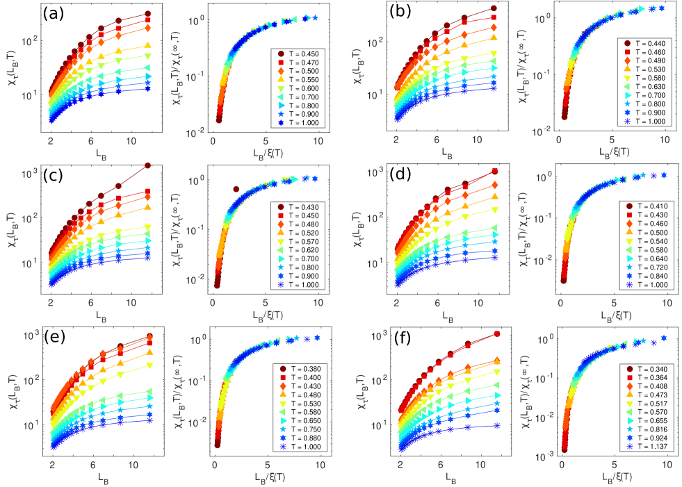
Figure S1: Block size dependence of $\chi_{\tau}$ and finite size scaling for activity $f_{0}$ = 0.0 (a), $f_{0}$ = 0.5 (b), $f_{0}$ = 1.0 (c), $f_{0}$ = 1.5 (d), $f_{0}$ = 2.0 (e) and $f_{0}$ = 2.5 (f)

As one increases the activity at constant temperature, the time scale of the glassy system decreases. To have our observation at a similar time scale for all range of activities, we have chosen a definite temperature window for each activity. We have performed all our MD simulations at that chosen temperature window for corresponding activity. First we used a newly proposed method called “block analysis”, which is considered an efficient method to perform finite-size scaling with a single sufficiently large system size data for obtaining the static length scale Chakrabarty et al. (2017). In this method, we have considered a small sub-system embedded in a moderately large system of fixed size. We referred these sub-systems as ‘blocks’ and the size of these can vary. Then we looked at the fluctuations of the $\tau_{\alpha}$ at every different size of these blocks and defined a quantity called $\chi_{\tau}$ (see definition later). For this method we carried all our simulation at a sufficiently large system size of $N=50000$ and constructed blocks of size $L_{B}=L/n$, where $n\in\{3,4,5,...\}$. We computed the $\tau_{\alpha}$ using the particles which are present inside one such box at a chosen time origin. Then we calculated the distribution of $\tau_{\alpha}$ as a function of different block size. For each block, we first measured the time at which the overlap correlation function $Q^{(i)}(L_{B},t)$ of a particular block for a fixed time origin attains a value of $1/e$. Here the subscript ‘$i$’ refers that the quantity is for a single block $i$ before performing any averaging. From this we further computed $\tau_{\alpha}^{(i)}(L_{B})$ and finally we calculated the mean and variance and defined $\chi_{\tau}(L_{B},T)$ such as,

$$\chi_{\tau}(L_{B},T)=L_{B}^{3}\left<\frac{\frac{1}{N_{B}}\sum_{i=1}^{N_{B}}[\Delta\tau_{\alpha}^{(i)}(L_{B})]^{2}}{[\overline{\tau_{\alpha}^{(i)}(L_{B})}]^{2}}\right>$$ (S2)

where,

$$\overline{\tau_{\alpha}^{(i)}(L_{B})}=\frac{1}{N_{B}}\sum_{i=1}^{N_{B}}\tau_{\alpha}^{(i)}(L_{B})$$ (S3)

and

$$\Delta\tau_{\alpha}^{(i)}(L_{B})=\tau_{\alpha}^{(i)}(L_{B})-\overline{\tau_{\alpha}^{(i)}(L_{B})}$$ (S4)

where $N_{B}$ is the number of blocks with size $L_{B}$, $n_{i}$, the number of particles in the $i$th block at time $t=0$.

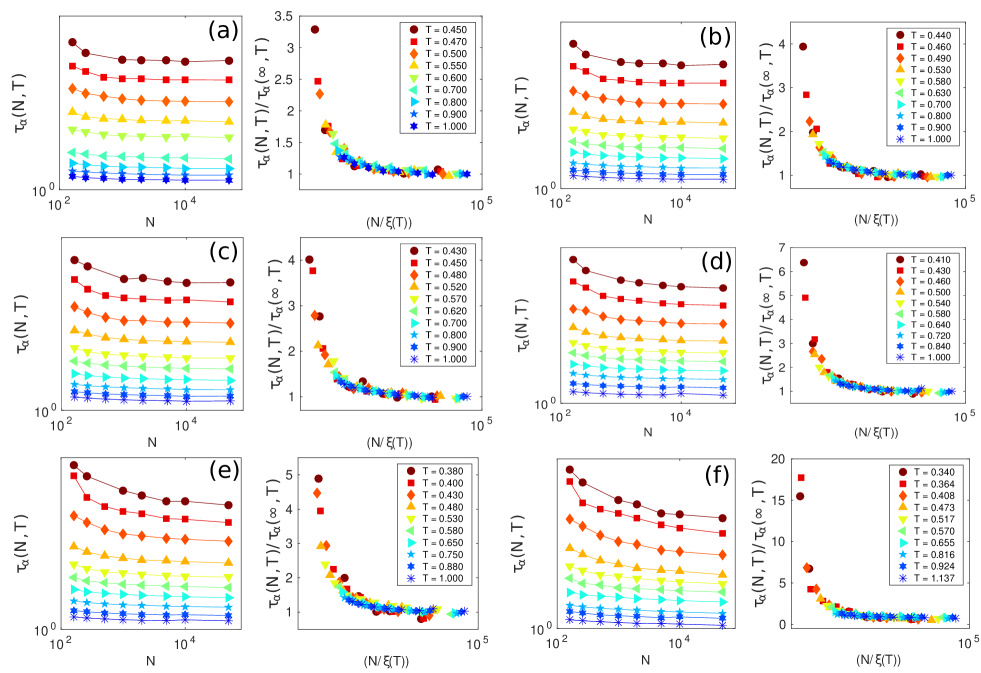
Figure S2: System size dependence of $\tau_{\alpha}$ and finite size scaling for activity $f_{0}$ = 0.0 (a), 0.5 (b), 1.0 (c), 1.5 (d), 2.0 (e) and 2.5 (f)

For every activity, we considered the variation of $\tau_{\alpha}$, $\chi_{\tau}$ at temperature $T$, on the block size $L_{B}$ for a fixed value of $N=\rho L^{3}$. This dependence of $\chi_{\tau}$ with different block size is shown in Fig.S1. The left panel of each sub figure shows the data for $\chi_{\tau}$ as a function of the block length $L_{B}$ at different temperature. $\chi_{\tau}$ at a given $T$ increases with $L_{B}$ and then saturates at some $T$-dependent value $\chi_{\tau}(\infty,T)$. This dependence of $\chi_{\tau}(L_{B},T)$ on $L_{B}$ is expected to exhibit the following Finite Size Scaling (FSS) form:

$$\chi_{\tau}(L_{B},T)=\chi_{0}(T)\mathcal{F}\left(\frac{L_{B}}{\xi_{S}}\right)$$ (S5)

where,

$$\chi_{0}(T)=\lim_{L_{B}\to\infty}\chi_{\tau}(L_{B},T)$$ (S6)

and $\xi_{S}$ is a characteristic scaling length scale. For each activity the data for all temperatures can be collapsed to a master curve using the two parameters $\chi_{\tau}(\infty,T)$ and $\xi_{S}$, as shown in right panel of each sub-figures of Fig. S1. The block size dependence of $\chi_{\tau}$ is governed by the length scale $\xi_{S}$. This length scale, extracted from this scaling collapse is the same as the static length scale, $\xi_{S}$, as shown in Karmakar et al. (2009) for the equilibrium glassy system. The excellent data collapse shown in Fig. S1 confirm that the extracted length scales will be very reliable with small error bars even in the non-equilibrium case.

S2.2 Finite size scaling of $\tau_{\alpha}$

We also performed the finite size scaling of $\tau_{\alpha}$ and extract the static length scale from it. To do this we performed the simulations varying the system size $N=160$ to $N=50000$ and computed the corresponding $\tau_{\alpha}$ for all temperatures, system sizes and activities. This dependence is shown in Fig.S2. The left panel of each sub figure shows the data for $\tau_{\alpha}$ as a function of system size $N$ for different temperatures. Fig.S2 shows that $\tau_{\alpha}$ at a given temperature decreases with $N$ and saturates at some $T$-dependent value $\tau_{\alpha}(\infty,T)$. Similarly the dependence of $\tau_{\alpha}(N,T)$ on $N$ is expected to exhibit the following Finite Size Scaling (FSS) form:

$$\tau_{\alpha}(N,T)=\tau_{0}(T)\mathcal{F}\left(\frac{N}{\xi_{S}}\right)$$ (S7)

where,

$$\tau_{0}(T)=\lim_{N\to\infty}\tau_{\alpha}(N,T)$$ (S8)

and $\xi_{S}$ is a characteristic scaling length scale. The data for all temperatures can be collapsed to a master curve using the two parameters $\tau_{\alpha}(\infty,T)$ and $\xi_{S}$, at each temperature, as shown in right panel of each sub-figures of Fig. S2 for different activities. This clearly show that the associated static length scale is consistently increasing with increasing activity at similar structural relaxation timescale.

S3 Temperature dependence of static length scale

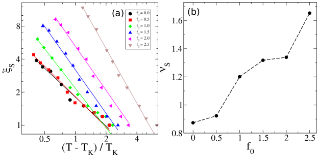
Figure S3: (a) Static length scale $\xi_{S}$ as a function of $(T-T_{K})/T_{K}$; lines are fits with the function $\xi_{S}\sim|(T-T_{K})/T_{K}|^{-\nu_{S}}$. (b) The exponent $\nu_{S}$ consistently increases with $f_{0}$.

Here we have presented the static length scale $\xi_{S}$ as a function of $|\frac{T-T_{K}}{T_{K}}|$ for different activities in Fig. S3(a) where $T_{K}$ is the Vogel-Fulcher-Tamman (VFT) divergence temperature, the temperature at which the relaxation time extrapolates to infinity. We obtained the value of $T_{K}$ by fitting the $\tau_{\alpha}(T)$ data at different $f_{0}$ with the VFT equation:

$$\tau_{\alpha}\sim\tau_{0}\exp{\left(\frac{A}{T-T_{K}}\right)}.$$

with $\tau_{0}$, $A$ and $T_{K}$ being the fitting parameters. Fig. S3(a) clearly shows that $\xi_{S}$ seems to show a power-law type divergence with temperature. We computed the exponent $\nu_{S}$ of this power law for each $f_{0}$ using the relation

$$\xi_{S}(T)\propto\left|\frac{T-T_{K}}{T_{K}}\right|^{-\nu_{S}}.$$

Fig. S3(b) shows the exponent $\nu_{S}$ as a function of $f_{0}$. The exponent is systematically increasing with increasing $f_{0}$.

Dependence of $\xi_{S}$ with $T_{g}/T$

We have also presented the static length scale, $\xi_{S}$, as a function of $T_{g}/T$ in Fig. S4, where $T_{g}$ is the calorimetric glass transition temperature and is defined as $\tau_{\alpha}(T=T_{g})=10^{6}$. It clearly shows that the static length scale $\xi_{S}$ is consistently increasing with increasing $f_{0}$ at similar range of $T_{g}/T$. Note that with increasing activity the system behaves as a strong liquid even though the static length scale shows stronger temperature dependence. This is very counter intuitive as in equilibrium systems, one finds the temperature dependence of the static length scale to be very mild for strong liquids whereas fragile liquid shows much stronger dependence on temperature Tah and Karmakar (2021). This clearly highlights a strong departure from effective equilibrium like behaviour in active glasses when one studies their static structural correlations even if the relaxation time can be described by an effective equilibrium theory.

Figure S4: Static length scale $\xi_{S}$ as a function of $T_{g}/T$ to demonstrate the dramatic growth of length scale within a comparable range of $T_{g}/T$, where $T_{g}$ is the calorimetric glass transition temperature, defined as $\tau_{\alpha}(T_{g})=10^{6}$.

References

- Kob and Andersen (1995) W. Kob and H. C. Andersen, Phys. Rev. E 51, 4626 (1995).
- Zhang (1997) F. Zhang, J. Chem. Phys. 106, 6102 (1997).
- Paul et al. (2021) K. Paul, S. K. Nandi, and S. Karmakar, arXiv: 2105.12702 (2021).
- Chakrabarty et al. (2017) S. Chakrabarty, I. Tah, S. Karmakar, and C. Dasgupta, Phys. Rev. Lett. 119, 205502 (2017).
- Karmakar et al. (2009) S. Karmakar, C. Dasgupta, and S. Sastry, Proc. Natl. Acad. Sci. (USA) 106, 3675 (2009).
- Tah and Karmakar (2021) I. Tah and S. Karmakar, arXiv:2108.02371 (2021).