Identification of the Source for Full Parabolic Equations

1 Introduction

The problem of source identification has been studied and analyzed in different areas of applied mathematics for the last decades. It has also received considerable attention from many current researchers in science and engineering. Applications can be found in problems related to heat conduction [8, 50],fissure identification [47], geophysical prospecting [2], contaminant detection [22] and tumor cell detection [24], to mention some.

The determination of sources turns out to be an ill-posed problem in the sense of Hadamard [13] since the solution does not depend continuously on the data.

Among the most significant tools used to determine a source, one can find in the literature the potential logarithmic method [28], the projective method [26], the Green function [15], dual reciprocity boundary element methods [10], the dual reciprocity method [34], the fundamental MFS solution method [16] and method by using the curve L [14].

Regarding the transport term in parabolic differential equations, there are no many articles published for the general case, most of the papers available in the literature focused on the heat equation. Sources of the heat equation are recovered using different methods and strategies, see for instance [11, 1, 17]. There are many articles that analyze particular cases with simplifications or restrictions on the mathematical models, the type of source, the border conditions or the chosen domain, like [11, 23, 32, 3, 42, 1, 17]. The most commonly used methods are limit element method [11, 17], MFS fundamental solution method [42, 1], Ritz-Galerkin method [31], differences method finite [44], non-mesh method [43], conditional stability method [37] and the firing method [23].

On the other hand, regularization methods [9, 19, 25] play an important role in the estimation of unstable solutions. The most widely used approaches are the iterative regularization method [18], the simplified method of regularization Tikhonov [12, 38, 4, 5], the modified regularization method [39, 45, 48], Fourier truncation [39], the method of mollification [41]. In particular for the determination of the source for a parabolic equation, certain regularization techniques are applied to specific transport equation. In [33] the authors focused on a convection-diffusion equation, while in [6, 7, 8, 35, 36, 45, 44, 48] only diffusion is considered.

Recently, the problem to find the source term as in this manuscript was solved by the quasi-reversibility method, see [27]. This method can be used to solve inverse source problem for nonlinear parabolic equations, the difference of this manuscript and that paper is the observation data [21].

This work aims to the determination, from noisy measurements taken at an arbitrary fixed time, of the real-valued function of n real variables, independent of time, in an evolutionary equation of transport in an unbounded domain. This is an ill-posed problem because the high frequency components of arbitrarily small data errors can lead to arbitrarily large errors in the solution [9, 19].

Here, a family of regularization operators is designed to compensate the factor that causes the instability of the inverse operator. The parametric regularization operators lead to a family of well-posed problems that approximates the given ill-posed problem. The regularization operator family proposed here turns out to be an $n$-dimensional generalization of the modified regularization method considered in [29, 30, 46, 40, 48]. In these articles the authors estimate the source of the one-dimensional equation of heat from data measured in a fixed moment of time $(t=1)$ by adding a penalizing term and the parameter choice rule depends on the norm of the unknown function. In contrast, this paper analyzes the general n-dimensional parabolic equation while relaxing the conditions on the assumptions for the regularization process.

The stability and convergence of this regularization method are analyzed and a Hölder type bound is derived for the estimation error. In order to illustrate the regularization performance, some numerical examples for the 1D, 2D and 3D cases are included.

2 The ill-posed mathematical framework

We consider the problem of determining the source $f$ for the following parabolic equation

$$\begin{cases}u_{t}({\mathbf{x}},t)=\alpha^{2}\Delta u(\mathbf{x},t)-\bm{\beta}\cdot\nabla(u(\mathbf{x},t))-\nu u(\mathbf{x},t)+f(\mathbf{x}),\qquad&\mathbf{x}\in\mathbb{R}^{n},\,t>0,\\ u(\mathbf{x},0)=0,\qquad&\mathbf{x}\in\mathbb{R}^{n},\\ u(\mathbf{x},t_{0})=y(\mathbf{x}),\qquad&\mathbf{x}\in\mathbb{R}^{n},\,t_{0}>0,\\ \end{cases}$$ (1)

where $\alpha^{2},\nu>0$,   $\bm{\beta}\in\mathbb{R}^{n}$ are given, $\Delta$ denotes the Laplacian operator, $\nabla$ denotes the Nabla operator and $``\cdot"$ is the usual inner product in $\mathbb{R}^{n}$. Note that this is a linear parabolic equations with constant coefficients. The existence and uniqueness of the solution to (1) is discussed in [49]. It is assumed that $u(\cdot,t),f(\cdot)\in L^{2}(\mathbb{R}^{n})$ are unknown functions and that $y\in L^{2}(\mathbb{R}^{n})$ can be measured with certain noise level $\delta$, i.e., the data function $y_{\delta}\in L^{2}(\mathbb{R}^{n})$ satisfies

$$||y-y_{\delta}||_{L^{2}(\mathbb{R}^{n})}\leq\delta,\qquad 0<\delta\leq\delta_{M},\\$$ (2)

where $\delta_{M}\in\mathbb{R}_{>0}$ represents the maximum level of noise. In practice , $\delta_{M}$ may be estimated from the error committed by the measuring instruments.

The analysis of the equation with boundary values and initial conditions in (1) is perform in the frequency space.

Definition 1.

Let $g\in L^{2}(\mathbb{R}^{n})$. The Fourier n-dimensional transform is defined

$$\hat{g}(\bm{\xi}):=\left(\frac{1}{\sqrt{2\pi}}\right)^{n}\int\limits_{\mathbb{R}^{n}}{e^{-i\bm{\xi}\cdot\mathbf{x}}\,g(\mathbf{x})\,d\mathbf{x}},\qquad\qquad\bm{\xi},\mathbf{x}\in\mathbb{R}^{n}.$$ (3)

By using the above definition (3), the system (1) can be written in the frequency space as

$$\begin{cases}\hat{u}_{t}(\bm{\xi},t)=-z(\bm{\xi})\,\hat{u}(\bm{\xi},t)+\hat{f}(\bm{\xi}),\qquad&\bm{\xi}\in\mathbb{R}^{n},\,t>0,\\ \hat{u}(\bm{\xi},0)=0,&\bm{\xi}\in\mathbb{R}^{n},\\ \hat{u}(\bm{\xi},t_{0})=\hat{y}(\bm{\xi}),&\bm{\xi}\in\mathbb{R}^{n},\,t_{0}>0,\end{cases}$$ (4)

where

$$z(\bm{\xi})=\alpha^{2}\|\bm{\xi}\|^{2}+i\,\bm{\beta}\cdot\bm{\xi}+\nu\,\in\mathbb{C}.$$

Solving (4) in the frequency space, we obtain the solution

$$\hat{u}(\bm{\xi},t)=\frac{1-e^{-z(\bm{\xi})\,t}}{z(\bm{\xi})}\hat{f}(\bm{\xi}).$$ (5)

Since $\hat{u}(\bm{\xi},t_{0})=\hat{y}(\bm{\xi})$, an expression for the source in the frequency space is obtained by evaluating the equation (5) in $t=t_{0}$, that is,

$$\hat{f}(\bm{\xi})=\Lambda(\bm{\xi})\hat{y}(\bm{\xi}),$$ (6)

where

$$\Lambda(\bm{\xi})=\frac{z(\bm{\xi})}{1-e^{-z(\bm{\xi})\,t_{0}}}.$$ (7)

Denoting $\hat{f_{\delta}}(\bm{\xi})=\Lambda(\bm{\xi})\hat{y_{\delta}}(\bm{\xi})$, we have

$$\|\hat{f}-\hat{f_{\delta}}\|_{L^{2}(\mathbb{R}^{n})}=\|\Lambda(\bm{\xi})(\hat{y}(\bm{\xi})-\hat{y_{\delta}}(\bm{\xi}))\|_{L^{2}(\mathbb{R}^{n})}=\|\Lambda(\bm{\xi})\|_{L^{2}(\mathbb{R}^{n})}\|\hat{y}(\bm{\xi})-\hat{y_{\delta}}(\bm{\xi})\|_{L^{2}(\mathbb{R}^{n})}.$$

Since

$$|\Lambda(\bm{\xi})| = \left|\frac{z(\bm{\xi})}{1-e^{-(\alpha^{2}\|\bm{\xi}\|^{2}+i\,\bm{\beta}\cdot\bm{\xi}+\nu)\,t_{0}}}\right|\geq\frac{|z(\bm{\xi})|}{1+e^{-(\alpha^{2}\|\bm{\xi}\|^{2}+\nu)\,t_{0}}\left|e^{-i\,\bm{\beta}\cdot\bm{\xi}\,t_{0}}\right|}$$ (8)

$$\geq \frac{|\alpha^{2}\|\bm{\xi}\|^{2}+\nu+i\,\bm{\beta}\cdot\bm{\xi}|}{1+e^{-(\alpha^{2}\|\bm{\xi}\|^{2}+\nu)\,t_{0}}},$$

$\Lambda(\bm{\xi})$ increases without bound as $\|\bm{\xi}\|\to\infty$ amplifying the high frequency components of the observation error $\hat{y}(\bm{\xi})-\hat{y}_{\delta}(\bm{\xi})$. This fact might lead to a large estimation error $\|\hat{f}-\hat{f_{\delta}}\|_{L^{2}(\mathbb{R}^{n})}$ even for small observation errors, hence one of the Hadamard conditions is not satisfied [13].

3 Regularization operators

In this section we propose a regularization operator taking into account the inestability factor in the inverse operator. We notice that the resulting operator is equivalent to the one that is obtained by using the quasi-reversibility method [20]. Basic theoretical issues related to regularization operators are included, more information can be found in [9, 19].

Definition 2.

Let $T:Y\longrightarrow X$, $X$ and $Y$ be Hilbert spaces and $T$ be an unbounded operator. A regularization strategy for $T$ is a family of linear and bounded operators

$$R_{\mu}:Y\longrightarrow X,\quad\mu>0,\quad/\quad\lim_{\mu\to 0^{+}}R_{\mu}y=Ty,\quad\forall y\in Y.\\$$ (9)

Let us define the parametric family of linear operators $R_{\mu}:L^{2}(\mathbb{R}^{n})\to L^{2}(\mathbb{R}^{n})$ for $\mu\in\mathbb{R}_{>0}$, by

$$R_{\mu}\hat{y}(\bm{\xi}):=\frac{\Lambda(\bm{\xi})}{1+\mu^{2}\|\bm{\xi}\|^{2}}\,\hat{y}(\bm{\xi}),$$ (10)

where $\Lambda(\bm{\xi})$ is given in (7) and $\mu$ is the regularization parameter. Note that the denominator in (10) was introduced for stabilization purposes. The properties for the operator family $\{R_{\mu},\,\mu>0\}$ are stated in the following theorem.

Theorem 1.

Let us consider the problem of identifying $f$ from noisy data $y_{\delta}(x)$ measured at a given time instant $t_{0}>0$, where $\delta$ is the noise level defined in (2). Let the functions $u$ and $f$ satisfy the following differential equation with initial condition

$$\begin{cases}u_{t}(\mathbf{x},t)=\alpha^{2}\Delta u(\mathbf{x},t)-\bm{\beta}\cdot\nabla(u(\mathbf{x},t))-\nu u(\mathbf{x},t)+f(\mathbf{x}),\qquad&\mathbf{x}\in\mathbb{R}^{n},\,t>0,\\ u(\mathbf{x},0)=0,\qquad&\mathbf{x}\in\mathbb{R}^{n},\\ \end{cases}$$ (11)

and let $\{R_{\mu}\}$ be the family of operators defined in (10). Then, for every $y(\mathbf{x})=u(\mathbf{x},t_{0})$ there exists an a-priori parameter choice rule for $\mu>0$ such that the pair $(R_{\mu},\mu)$ is a convergent regularization method for solving the identification problem (11).

Proof.

The factor $\displaystyle\frac{\Lambda(\bm{\xi})}{1+\mu^{2}\|\bm{\xi}\|^{2}}$ is bounded for all $\bm{\xi}$ since it is continuous for all $\bm{\xi}\in\mathbb{R}^{n}$ and

$$\begin{split}\lim_{\|\bm{\xi}\|\to\infty}\left|\frac{\Lambda(\bm{\xi})}{1+\mu^{2}\|\bm{\xi}\|^{2}}\right|=&\lim_{\|\bm{\xi}\|\to\infty}\left|\frac{\alpha^{2}\|\bm{\xi}\|^{2}+i\bm{\beta}\cdot\bm{\xi}+\nu}{(1-e^{-(\alpha^{2}\|\bm{\xi}\|^{2}+i\bm{\beta}\cdot\bm{\xi}+\nu)\,t_{0}})(1+\mu^{2}\|\bm{\xi}\|^{2})}\right|\\ =&\frac{\alpha^{2}}{\mu^{2}}<\infty.\end{split}$$

Hence, for $\mu>0$, $R_{\mu}$ is a linear continuous operator and we have that

$$\lim_{\mu\to 0^{+}}R_{\mu}\hat{y}=\Lambda\hat{y},$$

for $\hat{y}\in L^{2}(\mathbb{R}^{n})$, then $R_{\mu}$ is a regularization strategy for $\Lambda$. Therefore, by Proposition 3.4 in [9], for $y(\mathbf{x})=u(\mathbf{x},t_{0})$ there exists an a-priori parameter choice rule $\mu$ such that $(R_{\mu},\mu)$ is a convergent regularization method for solving (6). The regularized solution to the inverse problem in the frequency space is given by

$$\hat{f}_{\delta,\mu}=\frac{\Lambda(\bm{\xi})}{1+\mu^{2}\|\bm{\xi}\|^{2}}\,\hat{y}_{\delta}(\bm{\xi}).$$ (12)

Therefore, an estimated function to $f$ in (11) is given by the expression

$$f_{\delta,\mu}=\left(\frac{1}{\sqrt{2\pi}}\right)^{n}\int\limits_{\mathbb{R}^{n}}e^{i\bm{\xi}\cdot\mathbf{x}}R_{\mu}\hat{y}_{\delta}(\bm{\xi})\,d\bm{\xi}=\left(\frac{1}{\sqrt{2\pi}}\right)^{n}\int\limits_{\mathbb{R}^{n}}{e^{i\bm{\xi}\cdot\mathbf{x}}\frac{\Lambda(\bm{\xi})}{1+\mu^{2}\|\bm{\xi}\|^{2}}\,\hat{y}_{\delta}(\bm{\xi})\,d\bm{\xi}}.$$ (13)

4 Error analysis

In order to analyze the regularization performance, we first introduce some results that will be used later to obtain a bound for the error between the source $f(\mathbf{x})$ and its estimate $f_{\delta,\mu}(\mathbf{x})$, that we will be referred to as the regularization error.

Lemma 1.

For $\omega\in\mathbb{C}$ with $Re(\omega)>0$ holds $\displaystyle\left|\frac{1}{1-e^{-\omega}}\right|\leq\frac{1}{1-e^{-Re(\omega)}}.$

Proof.

Euler’s formula for a complex number $\omega=a+bi$, and the parity for sine and cosine yields $e^{-(a+bi)}=e^{-a}cos(b)-ie^{-a}sin(b)$. Then, adding and subtracting $2e^{-a}=2e^{-Re(\omega)}$, after algebraic operations one gets

$${|1-e^{-\omega}|^{2}=(1-e^{-Re(\omega)})^{2}+2e^{-Re(\omega)}(1-cos(Im(\omega)))}\geq(1-e^{-Re(\omega)})^{2}.$$

Hence

$$|1-e^{-\omega}|\geq 1-e^{-Re(\omega)}\Longrightarrow\displaystyle\left|\frac{1}{1-e^{-\omega}}\right|\leq\frac{1}{1-e^{-Re(\omega)}},$$

and the proof is completed

Lemma 2.

The function $f:\mathbb{R}_{>0}\to\mathbb{R}$ given by $\displaystyle f(x)=\begin{cases}\displaystyle\frac{x}{1-e^{-x}},&0<x<1,\\ \displaystyle\frac{1}{1-e^{-x}},&1\leq x,\end{cases}$ satisfies $f(x)\leq 2$.

Proof.

First, let us consider the function $f$ in $(0,1)$. Differentiating, in this case, we have $\displaystyle f^{\prime}(x)=\left(\frac{x}{1-e^{-x}}\right)^{\prime}=\displaystyle\frac{1+e^{-x}(-1+x)}{(1-e^{-x})^{2}}>0.$ Then the function $f$ is increasing in $(0,1)$ and $\displaystyle\frac{x}{1-e^{-x}}\leq\frac{1}{1-e^{-1}}.$
On the other hand, for $x>1$, $f^{\prime}(x)=\displaystyle\left(\frac{1}{1-e^{-x}}\right)^{\prime}=\displaystyle\frac{-e^{-x}}{(1-e^{-x})^{2}}<0,$ then $f$ is decreasing $\forall x>1$ and $\displaystyle\frac{1}{1-e^{-x}}\leq\frac{1}{1-e^{-1}}.$
Therefore we have that $\displaystyle f(x)<\frac{1}{1-e^{-1}}\,\,\forall x>0$ and since $\displaystyle\frac{1}{1-e^{-1}}\leq 2$ the proof is completed.

Lemma 3.

Let $\rho\in\mathbb{R}$. If $0<\mu<1$ we have $\displaystyle\frac{|\rho|}{1+\rho^{2}\mu^{2}}\leq\frac{1}{2\mu}.$ Moreover, for $\,\alpha^{2},\nu>0$ the following inequality holds $\displaystyle\frac{\alpha^{2}\rho^{2}+\nu}{1+\rho^{2}\mu^{2}}\leq\max\left\{\nu,\frac{\alpha^{2}}{\mu^{2}}\right\}.$

Proof.

Since $a^{2}+b^{2}\geq 2ab$ for all $a,b\in\mathbb{R}$, we have that

$$1+|\rho|^{2}\mu^{2}\geq 2|\rho|\mu\Longrightarrow\displaystyle\frac{|\rho|}{1+\rho^{2}\mu^{2}}\leq\frac{1}{2\mu}.$$

Now, let $\displaystyle k(\rho)=\frac{\alpha^{2}\rho^{2}+\nu}{1+\rho^{2}\mu^{2}}$, then $\displaystyle k^{\prime}(\rho)=\frac{2\rho(\alpha^{2}-\nu\mu^{2})}{(1+\rho^{2}\mu^{2})^{2}}$ and $k$ has only one critical point at $\rho=0$. Consider three cases:

• $\alpha^{2}=\nu\mu^{2}$: we have $k(\rho)=\nu$, constant $\forall\rho\in\mathbb{R}$.

• $\alpha^{2}<\nu\mu^{2}$: then the function $k$ reaches its global maximum value $\nu$ at $\rho=0$.
  

• $\alpha^{2}>\nu\mu^{2}$: since $k$ is an even function and it is increasing for $\rho>$0 with $\displaystyle\lim_{\rho\to\pm\infty}k(\rho)=\frac{\alpha^{2}}{\mu^{2}}$ we have $k(\rho)\leq\frac{\alpha^{2}}{\mu^{2}}$,

and the proof is completed.

Lemma 4.

For $\alpha^{2},\nu,t_{0}>0$,   $\bm{\beta}\in\mathbb{R}^{n}$ and $0<\mu<1$ we have that

$\displaystyle\left|\frac{\Lambda(\bm{\xi})}{1+\mu^{2}\|\bm{\xi}\|^{2}}\right|\leq\frac{2}{\mu^{2}}M$.

where $M=\max\left\{\frac{1}{t_{0}}+\frac{\sqrt{n}\|\bm{\beta}\|_{\infty}}{2\nu t_{0}};\nu+\alpha^{2}+\frac{\sqrt{n}\|\bm{\beta}\|_{\infty}}{2}\right\}$ and $\|\bm{\beta}\|_{\infty}=\max\limits_{1\leq j\leq n}|\bm{\beta}_{j}|.$

Proof.

From equation (7) and Lemma 1 we have

$$\left|\frac{\Lambda(\bm{\xi})}{1+\mu^{2}\|\bm{\xi}\|^{2}}\right|\leq\frac{\alpha^{2}\|\bm{\xi}\|^{2}+i\bm{\beta}\cdot\bm{\xi}+\nu}{(1-e^{-(\alpha^{2}\|\bm{\xi}\|^{2}+\nu)\,t_{0}})(1+\mu^{2}\|\bm{\xi}\|^{2})}.$$ (14)

If $(\alpha^{2}\|\bm{\xi}\|^{2}+\nu)\,t_{0}\geq 1$ : Using the triangular inequality, Lemmas 2 and 3

$$\begin{split}\phantom{space}\frac{\alpha^{2}\|\bm{\xi}\|^{2}+\nu+|\bm{\beta}\cdot\bm{\xi}|}{(1-e^{-(\alpha^{2}\|\bm{\xi}\|^{2}+\nu)\,t_{0}})(1+\|\bm{\xi}\|^{2}\mu^{2})}&\leq 2\left(\frac{\alpha^{2}\|\bm{\xi}\|^{2}+\nu}{1+\|\bm{\xi}\|^{2}\mu^{2}}+\frac{\sqrt{n}\|\bm{\beta}\|_{\infty}|\|\bm{\xi}\||}{1+\|\bm{\xi}\|^{2}\mu^{2}}\right)\\ &\leq 2\max\left\{\nu,\frac{\alpha^{2}}{\mu^{2}}\right\}+\frac{\sqrt{n}\|\bm{\beta}\|_{\infty}}{\mu}\\ &\leq\frac{2}{\mu^{2}}\left(\nu+\alpha^{2}+\frac{\sqrt{n}\|\bm{\beta}\|_{\infty}}{2}\right).\end{split}$$ (15)

If $(\alpha^{2}\|\bm{\xi}\|^{2}+\nu)\,t_{0}\in(0,1)$: Observe that

$$\phantom{space}\frac{\alpha^{2}\|\bm{\xi}\|^{2}+\nu+|\bm{\beta}\cdot\bm{\xi}|}{(1-e^{-(\alpha^{2}\|\bm{\xi}\|^{2}+\nu)\,t_{0}})(1+\|\bm{\xi}\|^{2}\mu^{2})}=\frac{(\alpha^{2}\|\bm{\xi}\|^{2}+\nu)\,t_{0}}{(1-e^{-(\alpha^{2}\|\bm{\xi}\|^{2}+\nu)\,t_{0}})(1+\|\bm{\xi}\|^{2}\mu^{2})\,t_{0}}$$

$$\hskip 56.9055pt+\frac{|\bm{\beta}\cdot\bm{\xi}|\,(\alpha^{2}\|\bm{\xi}\|^{2}+\nu)\,t_{0}}{(1-e^{-(\alpha^{2}\|\bm{\xi}\|^{2}+\nu)\,t_{0}})(1+\|\bm{\xi}\|^{2}\mu^{2})\,(\alpha^{2}\|\bm{\xi}\|^{2}+\nu)\,t_{0}}.$$

Using Lemmas 2 and 3

$$\begin{split}\frac{\alpha^{2}\|\bm{\xi}\|^{2}+\nu+|\bm{\beta}\cdot\bm{\xi}|}{(1-e^{-(\alpha^{2}\|\bm{\xi}\|^{2}+\nu)\,t_{0}})(1+\|\bm{\xi}\|^{2}\mu^{2})}&\\ \\ &\leq 2\left(\frac{1}{(1+\|\bm{\xi}\|^{2}\mu^{2})\,t_{0}}+\frac{|\bm{\xi}\cdot\bm{\beta}|}{(1+\|\bm{\xi}\|^{2}\mu^{2})(\alpha^{2}\|\bm{\xi}\|^{2}+\nu)\,t_{0}}\right)\\ \\ &\leq 2\left(\frac{1}{(1+\|\bm{\xi}\|^{2}\mu^{2})\,t_{0}}+\frac{\sqrt{n}\|\bm{\beta}\|_{\infty}}{2\mu(\alpha^{2}\|\bm{\xi}\|^{2}+\nu)\,t_{0}}\right)\qquad\qquad\\ \\ &\leq 2\left(\frac{1}{t_{0}}+\frac{\sqrt{n}\|\bm{\beta}\|_{\infty}}{2\mu\nu t_{0}}\right)\leq\frac{2}{\mu^{2}t_{0}}\left(1+\frac{\sqrt{n}\|\bm{\beta}\|_{\infty}}{2\nu}\right).\end{split}$$ (16)

Definition 3.

The norm in the Sobolev space $H^{p}(\mathbb{R}^{n}),\,p>0$ is defined as follows

$$\|f\|_{H^{p}(\mathbb{R}^{n})}:=\left(\,\,\int\limits_{\mathbb{R}^{n}}{|\hat{f}|^{2}\left(1+\|\bm{\xi}\|^{2}\right)^{p}\,d\bm{\xi}}\,\,\right)^{1/2}.$$ (17)

Theorem 2.

Consider the inverse problem of determining the source $f(\mathbf{x})$ in (1)-(2). Let $f_{\delta,\mu}(\mathbf{x})$ be the regularization solution given in (13) and assume that $\|f\|_{H^{p}(\mathbb{R}^{n})}<C$ ( $f$ is bounded in $H^{p}(\mathbb{R}^{n})$ for some $0<p<\infty$ (17)). Then choosing

$$\mu^{2}=\displaystyle\left(\frac{\delta}{C}\right)^{\frac{2}{p+2}},$$ (18)

we have

$$\|f-f_{\delta,\mu}\|_{L^{2}(\mathbb{R}^{n})}\leq 2\delta^{\frac{p}{p+2}}C^{\frac{2}{p+2}}\left[M+\frac{1}{2}\max\left\{1;\left(\frac{\delta}{C}\right)^{\frac{2-p}{p+2}}\right\}\right].$$ (19)

Proof.

From now on we denote $\|\cdot\|=\|\cdot\|_{L^{2}(\mathbb{R}^{n})}$.
Defining $\displaystyle\hat{f}_{\mu}(\bm{\xi}):=\frac{\Lambda(\bm{\xi})}{1+\mu^{2}\|\bm{\xi}\|^{2}}\hat{y}(\bm{\xi})$, by (6) it follows that

$$\begin{split}\left|\hat{f}(\bm{\xi})-\hat{f}_{\mu}(\bm{\xi})\right|=&\left|\hat{f}(\bm{\xi})\left(1-\frac{1}{1+\|\bm{\xi}\|^{2}\mu^{2}}\right)\frac{(1+\|\bm{\xi}\|^{2})^{\frac{p}{2}}}{(1+\|\bm{\xi}\|^{2})^{\frac{p}{2}}}\right|\\ \leq&\sup_{\|\bm{\xi}\|\in\mathbb{R}}\left|(1+\|\bm{\xi}\|^{2})^{-\frac{p}{2}}\left(1-\frac{1}{1+\|\bm{\xi}\|^{2}\mu^{2}}\right)\right|\left|\hat{f}(\bm{\xi})(1+\|\bm{\xi}\|^{2})^{\frac{p}{2}}\right|,\end{split}$$ (20)

and by the definition of the $H^{p}(\mathbb{R}^{n})$-norm given in (17), we have

$$\|\hat{f}(\bm{\xi})-\hat{f}_{\mu}(\bm{\xi})\|\leq\sup_{\|\bm{\xi}\|\in\mathbb{R}}\left|(1+\|\bm{\xi}\|^{2})^{-\frac{p}{2}}\left(1-\frac{1}{1+\|\bm{\xi}\|^{2}\mu^{2}}\right)\right|\|f\|_{H^{p}(\mathbb{R}^{n})}.$$ (21)

From the triangle inequality,

$$\|\hat{f}-\hat{f}_{\delta,\mu}\|\leq\|\hat{f}-\hat{f}_{\mu}\|+\|\hat{f}_{\mu}-\hat{f}_{\delta,\mu}\|,$$ (22)

then (21)-(22) and the definition of the regularized source (12) yield to

$\left\|\hat{f}-\hat{f}_{\delta,\mu}\right\|\leq$	$\sup\limits_{\|\bm{\xi}\|\in\mathbb{R}}\left|(1+\|\bm{\xi}\|^{2})^{-\frac{p}{2}}\left(1-\frac{1}{1+\|\bm{\xi}\|^{2}\mu^{2}}\right)\right|\|f\|_{H^{p}(\mathbb{R}^{n})}$
	$+\sup\limits_{\|\bm{\xi}\|\in\mathbb{R}}\left|\frac{\Lambda(\bm{\xi})}{1+\|\bm{\xi}\|^{2}\mu^{2}}\right|\left\|\hat{y}-\hat{y}_{\delta}\right\|.$

From [45], $\displaystyle\sup_{\|\bm{\xi}\|\varepsilon\mathbb{R}}\left|(1+\|\bm{\xi}\|^{2})^{-\frac{p}{2}}\left(1-\frac{1}{1+\|\bm{\xi}\|^{2}\mu^{2}}\right)\right|\leq\max\left\{\mu^{p},\mu^{2}\right\},$ this result together with Lemma 4 and the assumption $\left\|\hat{y}-\hat{y}_{\delta}\right\|\leq\delta$ lead to

$$\|\hat{f}-\hat{f}_{\delta,\mu}\|\leq\max\left\{\mu^{p},\mu^{2}\right\}\|f\|_{H^{p}(\mathbb{R}^{n})}+\frac{2\delta}{\mu^{2}}M.$$

Choosing $\mu^{2}=\displaystyle\left(\frac{\delta}{C}\right)^{\frac{2}{p+2}}$, by Parseval’s identity and the linearity of the Fourier transform,

$$\|f-f_{\delta,\mu}\|=\left\|\hat{f}-\hat{f}_{\delta,\mu}\right\|\leq\max\left\{\delta^{\frac{p}{p+2}}C^{\frac{2}{p+2}};\delta^{\frac{2}{p+2}}C^{\frac{p}{p+2}}\right\}+2M\delta^{\frac{p}{p+2}}C^{\frac{2}{p+2}},$$

equivalently

$$\|f-f_{\delta,\mu}\|_{L^{2}(\mathbb{R}^{n})}\leq 2\delta^{\frac{p}{p+2}}C^{\frac{2}{p+2}}\left[M+\frac{1}{2}\max\left\{1;\left(\frac{\delta}{C}\right)^{\frac{2-p}{p+2}}\right\}\right].$$ (23)

A-priori regularization parameter is usually chosen to be dependent on a-prior bound for the $H^{p}$ norm of the source and data noise. For the numerical examples the bound is generally assumed to be 1 [29, 30, 46, 40, 48] which can lead to erroneous estimates when $\|f\|_{H^{p}(\mathbb{R}^{n})}>1$.

Here, we include a rule of choice for the regularization parameter that only depends on data noise. The following theorem is aimed to the estimate error for this case.

Theorem 3.

Consider the inverse problem of determining the source $f(\mathbf{x})$ in (1)-(2). Let $f_{\delta,\mu}(\mathbf{x})$ be the regularization solution given in (13) and assume that $\|f\|_{H^{p}(\mathbb{R}^{n})}$ is bounded in $H^{p}(\mathbb{R}^{n})$ for some $0<p<\infty$(17). Then choosing

$$\mu^{2}=\displaystyle\delta^{\frac{2}{p+2}},$$ (24)

there exists a constant $K$ independent of $\delta$ such that

$$\|f-f_{\delta,\mu}\|_{L^{2}(\mathbb{R}^{n})}\leq K\,\max\left\{\delta^{\frac{2}{p+2}};\delta^{\frac{p}{p+2}}\right\}.$$ (25)

Proof.

From now on we denote $\|\cdot\|=\|\cdot\|_{L^{2}(\mathbb{R}^{n})}$. From the proof of Theorem 2 we have that $\|\hat{f}-\hat{f}_{\delta,\mu}\|\leq\max\left\{\mu^{p},\mu^{2}\right\}\|f\|_{H^{p}(\mathbb{R}^{n})}+\frac{2\delta}{\mu^{2}}M.$ Choosing $\mu^{2}=\displaystyle\delta^{\frac{2}{p+2}}$, by Parseval’s identity and the linearity of the Fourier transform,

$$\|f-f_{\delta,\mu}\|=\left\|\hat{f}-\hat{f}_{\delta,\mu}\right\|\leq K\max\left\{\delta^{\frac{2}{p+2}},\delta^{\frac{p}{p+2}}\right\}.$$ (26)

where $K=C+2M=C+2\max\left\{\frac{1}{t_{0}}+\frac{\sqrt{n}\|\bm{\beta}\|_{\infty}}{2\nu t_{0}};\nu+\alpha^{2}+\frac{\sqrt{n}\|\bm{\beta}\|_{\infty}}{2}\right\}$ and $C$ is the bound for the $H^{p}(\mathbb{R}^{n})$-norm of $f$, i.e., $\|f\|_{H^{p}(\mathbb{R}^{n})}\leq C$.

Remark 1.

Note $p=\infty$ is excluded since and the error bound in that case the error bound is $K$.

A particular case of mathematical interest is for $p=2$, where we obtain

$$\|f-f_{\delta,\mu}\|\leq K\sqrt{\delta}.$$

Remark 2.

If a bound ${\delta_{M}}>1$ is allowed for noise in measurements, in order to keep $0<\mu<1$ one can take

$$\mu^{2}=\displaystyle\left(\frac{\delta}{\delta_{M}}\right)^{\frac{2}{p+2}}.$$ (27)

In that case, for $K=C+2\,\displaystyle{\delta_{M}}^{\frac{4}{p+2}}\max\left\{\frac{1}{t_{0}}+\frac{\sqrt{n}\|\bm{\beta}\|_{\infty}}{2\nu t_{0}};\nu+\alpha^{2}+\frac{\sqrt{n}\|\bm{\beta}\|_{\infty}}{2}\right\}$ we have $\|f-f_{\delta,\mu}\|=\left\|\hat{f}-\hat{f}_{\delta,\mu}\right\|\leq K\max\left\{\left(\frac{\delta}{\delta_{M}}\right)^{\frac{2}{p+2}};\left(\frac{\delta}{\delta_{M}}\right)^{\frac{p}{p+2}}\right\}.$

5 Numerical examples

In this section we consider few examples with a source $f\in\mathbb{R}^{n},n=1,2,3$ to illustrate the performance of the regularization operator. For each of them we have chosen different values for the parameters $\alpha^{2},\bm{\beta},\nu$, $t_{0}$ and a set of standard deviation values $\{\epsilon_{1},...,\epsilon_{k}\}$ for the data noise. The space is uniformly discretized and a data set $\{y_{\delta_{1}},...,y_{\delta_{N}}\}$ is obtained by evaluating the solution $u(\mathbf{x},t)$ at a fixed time instant $t_{0}$ and adding noise, that is,

$$y_{\delta_{i}}=y(\mathbf{x}_{i})+\epsilon_{i},\quad i=1,...,N,\,\,\mathbf{x}_{i}\in{\cal G},$$ (28)

where ${\cal G}$ is the uniform grid defined on $\mathbb{R}^{n}$ and $\epsilon_{i},i=1,...,N$ are realizations of the normally distributed random variable ${\eta}$ with mean 0 and standard deviation $\epsilon$.

By denoting $y_{i}=y(\mathbf{x}_{i}),i=1,..,N$, since the noise level $\delta$ satisfies (2), the error

$$\mathbf{y}-\mathbf{y}_{\delta}=(y_{1}-y_{\delta_{1}},...,y_{N}-y_{\delta_{N}})=(\epsilon_{1},...,\epsilon_{N}),$$ (29)

is numerically integrated using the Simpson’s method to obtained an approximated value for $\delta=\delta(\epsilon)$. Then $\delta_{M}$ in (2) is chosen to be an upper bound for $\delta$. In practice, $\delta_{M}$ can be estimated based on the measuring instruments used in data collection.

Afterwards,$\{\hat{y}_{\delta_{1}},...,\hat{y}_{\delta_{N}}\}$ is calculated by means of the FFT (Fast Fourier Transform) and the regularized solution $f_{\delta,\mu}$ is calculated as defined in (13) using the inverse FFT [8] where the regularization parameter $\mu$ is chosen according to (27).

The results of the estimated sources (non-regularized and the regularized one) are plotted. A table of errors is included for each example which shows the absolute and relative errors. For comparison purposes, the errors for all the examples are calculated taking (29) $\{\epsilon_{1},...,\epsilon_{5}\}=\{0.01,0.03,0.05,0.08,0.1\}$.

Remark 3.

Notice that in some examples a good estimation is obtained even when the parameter value $p$ does not correspond to the $H^{p}$ space where the source belongs.

5.1 Examples 1D

Two examples are considered for the one-dimensional inverse source problem defined in (1).

Example 1.

For this example the source $f$ is defined by

$$f(x)=\begin{cases}-1,\qquad&-20\leq x<-10,\\ 1,\qquad&-10\leq x<0,\\ -1,\qquad&0\leq x<10,\\ 1,\qquad&10\leq x\leq 20,\\ 0,\qquad&\text{in another case}.\end{cases}$$

With modeling parameter values $\alpha^{2}=2.10^{-5},\bm{\beta}=1.10^{-5},\nu=1,t_{0}=5,p=1$ and $\epsilon\in\{0.2,0.15,0.1,0.05\}$.

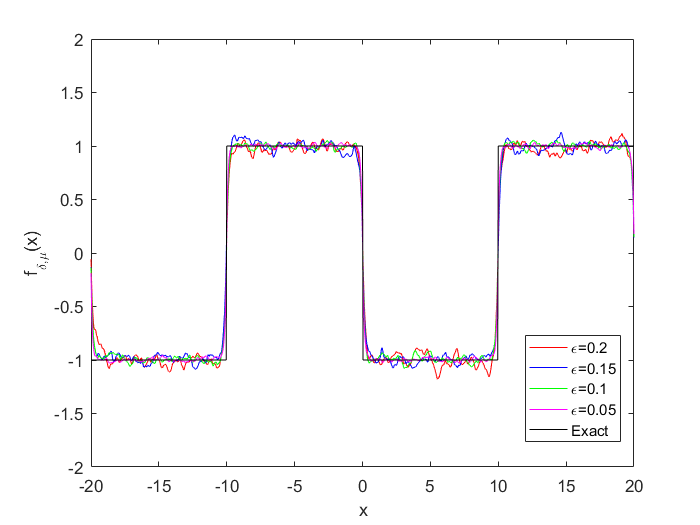
(a)	(b)

Figure 1: Sources for example 1: unregularized (a) and regularized (b) assuming $\alpha^{2}=2.10^{-5},\bm{\beta}=1.10^{-5},\nu=1,t_{0}=5,p=1$ and $\epsilon\in\{0.2,0.15,0.1,0.05\}$.

Table 1: Example 1: Errors assuming $\alpha^{2}=2.10^{-5},\bm{\beta}=1.10^{-5},\nu=1,t_{0}=1,p=1$.

Absolute errors	Relative errors
$\epsilon$ $\|f-f_{\delta}\|$ $\|f-f_{\delta,\mu}\|$ 0.01 0.4610 0.0998 0.03 0.5750 0.2985 0.05 0.6430 0.4853 0.08 0.8268 0.7000 0.1 0.9512 0.7445	$\|f-f_{\delta}\|/\|f\|$ $\|f-f_{\delta,\mu}\|/\|f\|$ 0.0729 0.0158 0.0909 0.0472 0.1017 0.0767 0.1307 0.1107 0.1504 0.1177

Example 2.

For this example the source $f$ is defined by

$$f(x)=\begin{cases}x+1,\qquad&-1\leq x<0,\\ -x+1,\qquad&0\leq x\leq 1,\\ 0,\qquad&\text{in another case}.\end{cases}$$

With modeling parameter values $\alpha^{2}=2,\bm{\beta}=0,\nu=1,t_{0}=0.2,p=2$ and $\epsilon\in\{0.004,0.003,0.002,0.001\}$.

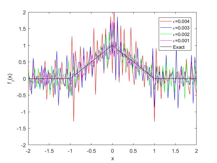
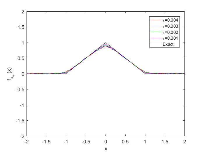
(a)	(b)

Figure 2: Sources for example 2: unregularized (a) and regularized (b) assuming $\alpha^{2}=2,\bm{\beta}=0,\nu=1,t_{0}=0.2,p=2$ and $\epsilon\in\{0.004,0.003,0.002,0.001\}$.

Table 2: Example 2: Errors assuming $\alpha^{2}=2,\bm{\beta}=0,\nu=1,t_{0}=1,p=1$.

Absolute errors	Relative errors
$\epsilon$ $\|f-f_{\delta}\|$ $\|f-f_{\delta,\mu}\|$ 0.01 2.5927 0.1698 0.03 9.4906 0.2559 0.05 12.9565 0.2878 0.08 23.9564 0.3579 0.1 25.1220 0.3713	$\|f-f_{\delta}\|/\|f\|$ $\|f-f_{\delta,\mu}\|/\|f\|$ 3.1728 0.2077 11.6143 0.3131 15.8558 0.3522 29.7091 0.4380 30.7802 0.4512

5.2 Examples 2D

Two examples are considered for the two-dimensional inverse source problem defined in (1).

Example 3.

For this example the source $f$ is defined by

$$f(x)=\begin{cases}\ cos\left(\frac{x_{1}}{20}\right)\ cos\left(\frac{x_{2}}{20}\right),\qquad&-40\leq x_{1},x_{2}\leq 40,\\ 0,\qquad&\text{in another case}.\end{cases}$$

With modeling parameter values $\alpha^{2}=0.2,\bm{\beta}=(0,0),\nu=0.999,t_{0}=1,p=1$ and $\epsilon=0.025$.

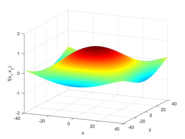
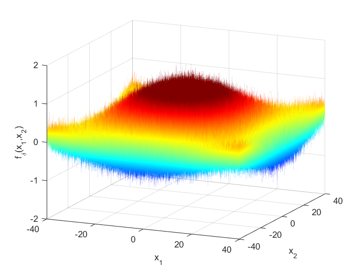
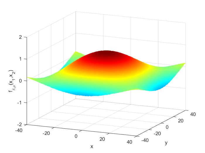
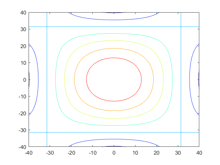
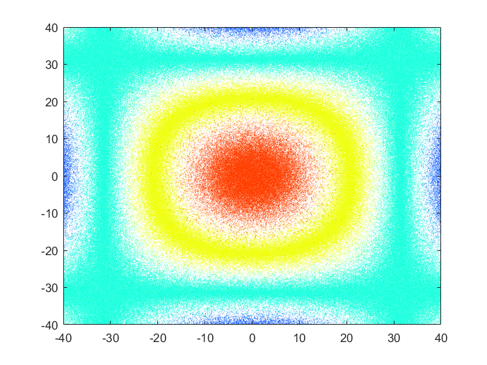
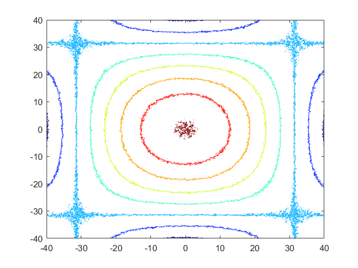
(a)	(b)	(c)

Figure 3: Sources for example 3: original (a), unregularized (b) and regularized (c) assuming $\alpha^{2}=0.2,\bm{\beta}=(0,0),\nu=0.999,t_{0}=1,p=1$ and $\epsilon=0.025$.

Table 3: Example 3: Errors assuming $\alpha^{2}=0.2,\bm{\beta}=(0,0),\nu=0.999,t_{0}=1,p=1$.

Aboslute errors	Relative errors
$\epsilon$ $\|f-f_{\delta}\|$ $\|f-f_{\delta,\mu}\|$ 0.01 5.6563 0.2599 0.03 16.9395 0.7778 0.05 28.2357 1.3021 0.08 45.1974 2.0774 0.1 56.3882 5.5962	$\|f-f_{\delta}\|/\|f\|$ $\|f-f_{\delta,\mu}\|/\|f\|$ 0.1744 0.0008 0.5221 0.0240 0.8706 0.0401 1.3936 0.0641 1.7387 0.0800

Example 4.

For this example the source $f$ is defined by

$$f(x_{1},x_{2})=\begin{cases}10+x_{1}-x_{2},\qquad&-10\leq x_{1}\leq 0,\,\,\,\,\,\,0\leq x_{2}\leq 10+x_{1},\\ 10+x_{1}+x_{2},\qquad&-10\leq x_{1}\leq 0,\,\,\,\,\,\,-10-x_{1}\leq x_{2}\leq 0,\\ 10-x_{1}-x_{2},\qquad&0\leq x_{1}\leq 10,\,\,\,\,\,\,0\leq x_{2}\leq 10-x_{1},\\ 10-x_{1}+x_{2},\qquad&10\leq x_{1}\leq 10,\,\,\,\,\,\,-10+x_{1}\leq x_{2}\leq 0,\\ 0,\qquad&\text{in another case}.\end{cases}$$

With modeling parameter values $\alpha^{2}=1,\bm{\beta}=(0,0),\nu=1,t_{0}=0.4,p=0.6$ and $\epsilon=0.05$.

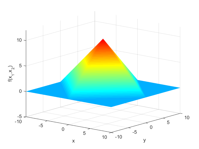
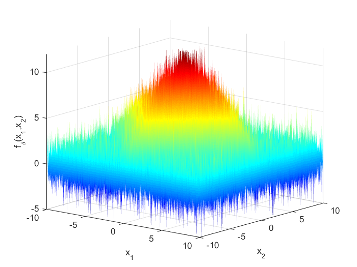
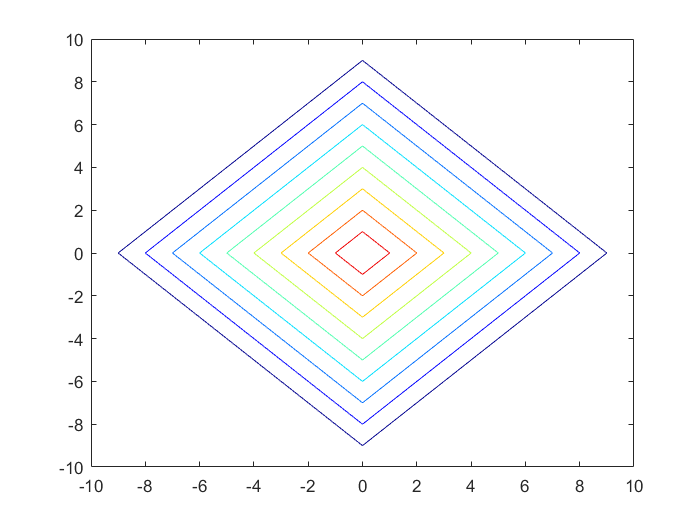
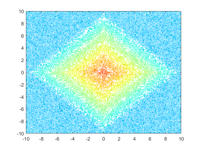
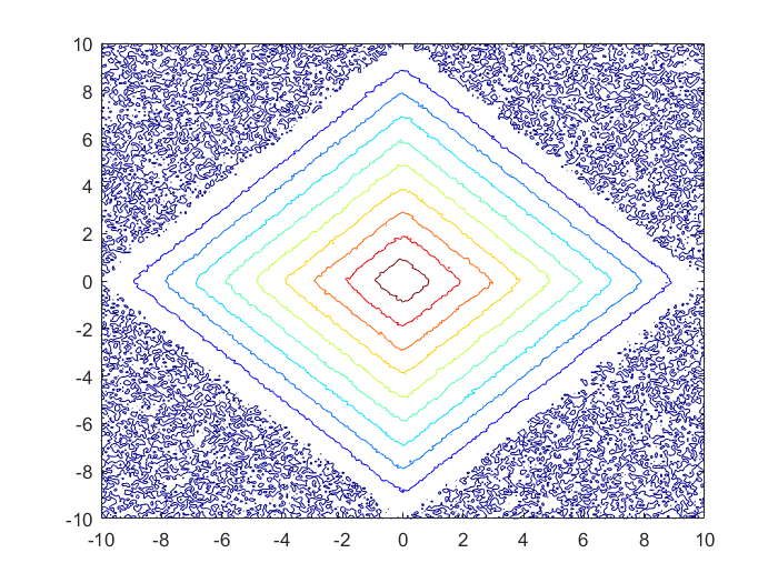
(a)	(b)	(c)

Figure 4: Sources for example 4: original (a), unregularized (b) and regularized (c) assuming $\alpha^{2}=1,\bm{\beta}=(0,0),\nu=1,t_{0}=0.4,p=0.6$ and $\epsilon=0.05$.

Table 4: Example 4: Errors assuming $\alpha^{2}=1,\bm{\beta}=(0,0),\nu=1,t_{0}=1,p=1$.

Aboslute errors	Relative errors
$\epsilon$ $\|f-f_{\delta}\|$ $\|f-f_{\delta,\mu}\|$ 0.01 6.5149 0.3527 0.03 19.2785 0.6748 0.05 31.7283 1.0502 0.08 50.7739 1.6429 0.1 63.9207 2.0451	$\|f-f_{\delta}\|/\|f\|$ $\|f-f_{\delta,\mu}\|/\|f\|$ 0.1128 0.0061 0.3339 0.0117 0.5496 0.0182 0.8796 0.0285 1.1071 0.0354

5.3 Examples 3D

One example are considered for the three-dimensional inverse source problem defined in (1).

Example 5.

For this example the source $f$ is defined by

$$f(x)=\begin{cases}\ sin\left(\frac{x_{1}+x_{2}+x_{3}}{20}\right),\qquad&-2\pi\leq x_{1},x_{2},x_{3}\leq 2\pi,\\ 0,\qquad&\text{in another case}.\end{cases}$$

With modeling parameter values $\alpha^{2}=0.4,\bm{\beta}=(1,-0.5,-0.5),\nu=0.997,t_{0}=3,p=3$ and $\epsilon=0.035$. For this case, we consider either $x=0$, $y=0$ or $z=0$ to plot the resulting estimated sources, the non-regularized and the regularized one.

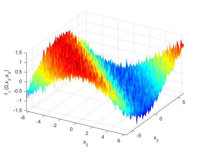
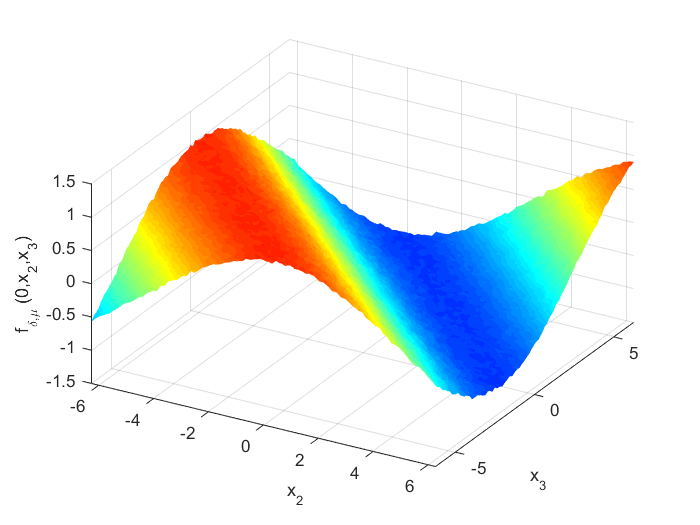
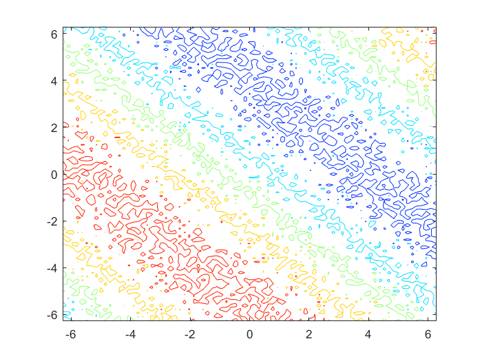
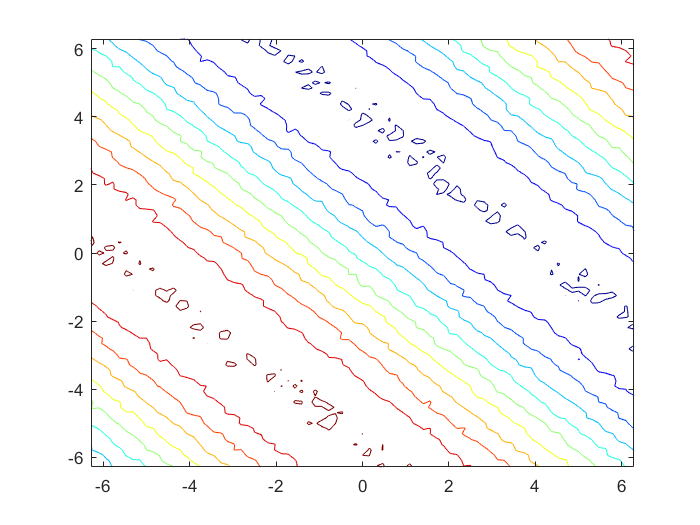
(a)	(b)	(c)

Figure 5: Sources for example 5: original (a), unregularized (b) and regularized (c) for $x=0$ assuming $\alpha^{2}=0.4,\bm{\beta}=(1,-0.5,-0.5),\nu=0.997,t_{0}=3,p=3$ and $\epsilon=0.035$.

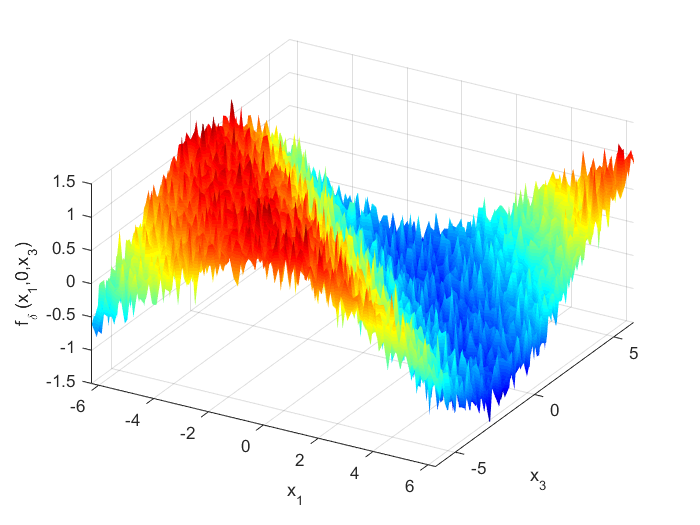
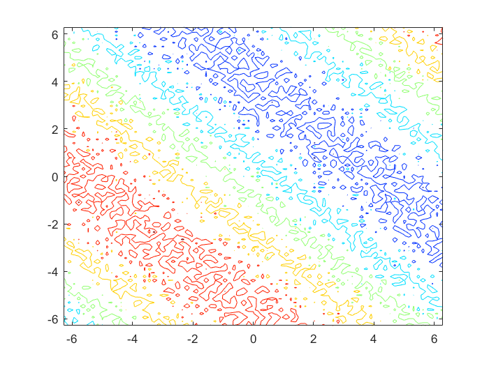
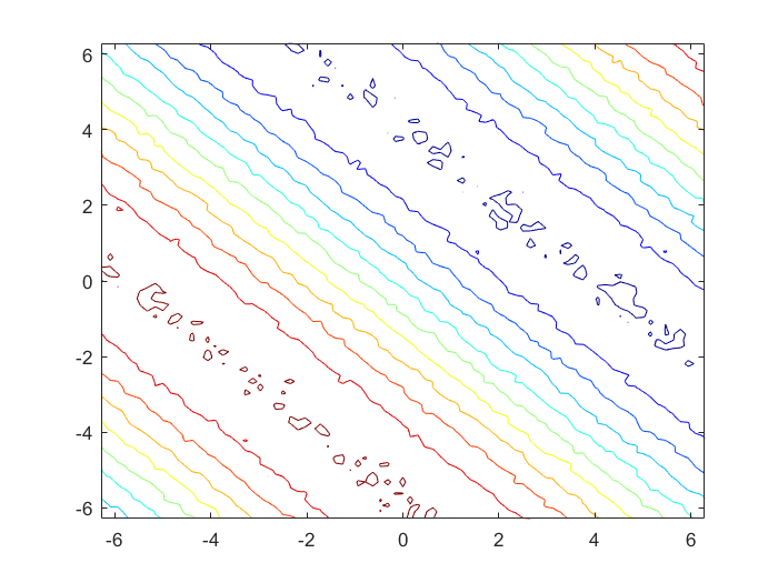
(a)	(b)	(c)

Figure 6: Sources for example 5: original (a), unregularized (b) and regularized (c) for $y=0$ assuming $\alpha^{2}=0.4,\bm{\beta}=(1,-0.5,-0.5),\nu=0.997,t_{0}=3,p=3$ and $\epsilon=0.035$.

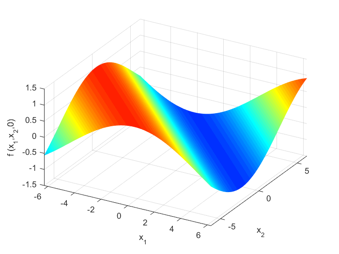
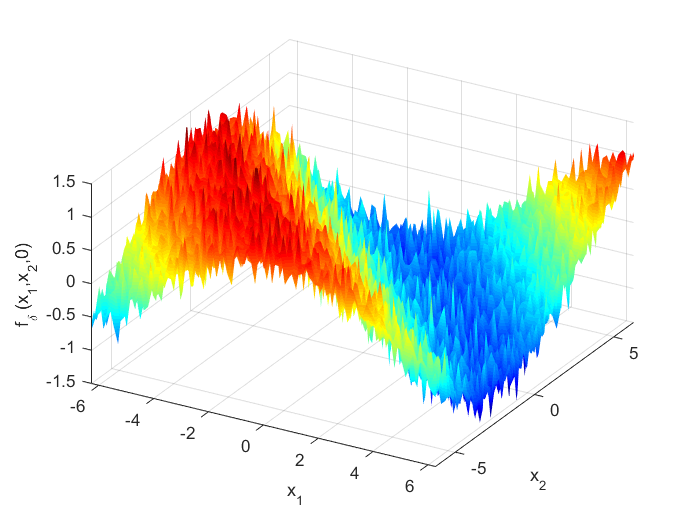
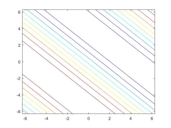
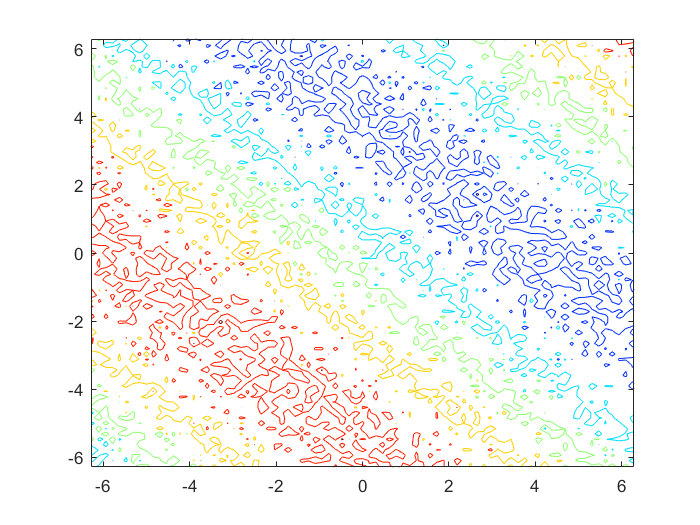
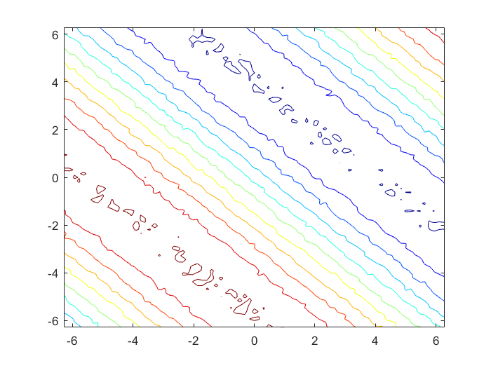
(a)	(b)	(c)

Figure 7: Sources for example 5: original (a), unregularized (b) and regularized (c) for $z=0$ assuming $\alpha^{2}=0.4,\bm{\beta}=(1,-0.5,-0.5),\nu=0.997,t_{0}=3,p=3$ and $\epsilon=0.035$.

Table 5: Example 5: Errors assuming $\alpha^{2}=0.4,\bm{\beta}=(1,-0.5,-0.5),\nu=0.997,t_{0}=1,p=1$.

Aboslute errors	Relative errors
$\epsilon$ $\|f-f_{\delta}\|$ $\|f-f_{\delta,\mu}\|$ 0.01 2.7377 0.3890 0.03 8.2057 0.7947 0.05 13.6597 1.2621 0.08 21.9170 1.9791 0.1 27.3875 2.4679	$\|f-f_{\delta}\|/\|f\|$ $\|f-f_{\delta,\mu}\|/\|f\|$ 0.0842 0.0120 0.2522 0.0244 0.4149 0.0388 0.6737 0.0608 0.8419 0.0759

6 Conclusion

This work focus on the problem of the inverse source for full parabolic equations in $\mathbb{R}^{n}.$ A family of regularization operators is defined in order to deal with the ill-posedness the problem. It was designed to compensate the instability factor in the inverse operator. A rule of choice for the regularization parameters is also included which is based on the noise level assumed in the data set and the smoothness of the source to be identified. We demonstrate that for the parameter choice rule proposed here, the method is stable and a bound of Hölder type is obtained for the regularization error.

The numerical examples show good estimates for the different n-variables sources, $n=1,2,3$, determined from data with different noise levels. Moreover, the sources used for the numerical examples belong to different Hilbert spaces and all of them show a good performance of the regularization approach adopted.

Acknowledgements: I thank Diana Rubio for her valuable and selfless collaboration.

Funding: This work was partially supported by SOARD/AFOSR through grant FA9550-18-1-0523, CONICET graduate scholarship and UNGS research assistantship.

References:

- [1] Ahmadabadi, M., Arab, M. and Maalek Ghaini, F.M. The method of fundamental solutions for the inverse space-dependent heat source problem. Engineering Analysis with Boundary Elements. 33(10):1231–1231, 2009. 10.1016/j.enganabound.2009.05.001
- [2] Beroza, G.C. and Spudich, P. Linearized inversion for fault rupture behavior: application to the 1984 Morgan Hill, California, earthquake. Journal of Geophysical Research: Solid Earth. 93(6):6275–6296, 1988. 10.1029/jb093ib06p06275
- [3] Cannon, J.R. and Duchateau, P. Structural identification of an unknown source term in a heat equation. Inverse Problems. 14(3):535–551, 1998. 10.1088/0266-5611/14/3/010
- [4] Cheng, W., Fu, C.L. and Qian, Z. A modified Tikhonov regularization method for a spherically symmetric three-dimensional inverse heat conduction problem. Mathematics and Computers in Simulation. 75(3):97–112, 2007. 10.1016/j.matcom.2006.09.005
- [5] Cheng, W., Fu, C.L. and Qian, Z. Two regularization methods for a spherically symmetric inverse heat conduction problem. Applied Mathematical Modelling. 32(4):432–442, 2008. 10.1016/j.apm.2006.12.012
- [6] Dou, F.F. and Fu, C.L. Determining an unknown source in the heat equation by a wavelet dual least squares method. Applied Mathematics Letters. 22(5):661–667, 2009. 10.1016/j.aml.2008.08.003
- [7] Dou, F.F., Fu, C.L. and Yang, F-L. Optimal error bound and Fourier regularization for identifying an unknown source in the heat equation. Journal of Computational and Applied Mathematics 230(2):728–737, 2009. 10.1016/j.cam.2009.01.008
- [8] Eldén, L., Berntsson, F. and Reginska, T. Wavelet and Fourier methods for solving the sideways heat equation. SIAM Journal on Scientific Computing 21(6):2187–2205, 2000. 10.1137/s1064827597331394
- [9] Engel, H., Hanke, M. and Neubauer, A. Regularization of Inverse Problems. Kluwer Academic Publisher, 1996.
- [10] Farcas, A., Elliott, L., Ingham, D.B., Lesnic, D. and Mera, S. A dual reciprocity boundary element method for the regularized numerical solution of the inverse source problem associated to the Poisson equation. Inverse Problems in Engineering 11(2):123–139, 2003. 10.1080/1068276031000074267
- [11] Farcas, A. and Lesnic, D. The boundary-element method for the determination of a heat source dependent on one variable. Journal of Engineering Mathematics 54(4):375–388, 2006. 10.1007/s10665-005-9023-0
- [12] Fu, C.L. Simplified Tikhonov and Fourier regularization methods on a general sideways parabolic equation. Journal of Computational and Applied Mathematics 167(2):449–463, 2004. 10.1016/s0377-0427(03)00932-4
- [13] Hadamard, J. Lectures on Cauchy problem in linear Differential Equations. Yale University Press , New Haven, 1923.
- [14] Hansen, C. and O’Leary, A.P. The use of the L-curve in the regularization of discrete ill-posed problems. SIAM Journal on Scientific Computing 14(6):1487–1503, 1993. 10.1137/0914086
- [15] Hon, Y.C., Li, M. and Melnikov, Y.A. Inverse source identification by Green’ s function. Engineering Analysis with Boundary Elements 34(4):352–358, 2010. 10.1016/j.enganabound.2009.09.009
- [16] Jin, B. and Marin, L. The method of fundamental solutions for inverse source problems associated with the steady-state heat conduction. International Journal for Numerical Methods in Engineering 69(8):1570–1589, 2007. 10.1002/nme.1826
- [17] Johansson, B.T. and Lescnic, D. Determination of a spacewise dependent heat source. Journal of Computational and Applied Mathematics 209(1):66–80, 2007. 10.1016/j.cam.2006.10.026
- [18] Johansson, B.T. and Lescnic, D. A procedure for determining a spacewise dependent heat source and the initial temperature. Applicable Analysis 87(3):265–276, 2008. 10.1080/00036810701858193
- [19] Kirsch, A. An introduction to the mathematical theory of inverse problems. Springer, 2011.
- [20] Lattès, R. and Lions, J.L. The method of quasi-reversibility: applications to partial differential equations. Elservier, New York, 1969.
- [21] Le, T.T. and Nguyen, L.H. A convergent numerical method to recover the initial condition of nonlinear parabolic equations from lateral Cauchy data. Journal of Inverse and Ill-posed Problems 14(3):287–300, 2020. 10.1515/jiip-2020-0028
- [22] Tan, G.S., Cheng Y.J. and Wang, X.Q. Determining magnitude of groundwater pollution sources by data compatibility analysis. Inverse Problems in Science and Engineering 14(3):287–300, 2006. 10.1080/17415970500485153
- [23] Liu, C.S. An two-stage LGSM to identify time dependent heat source through an internal measurement of temperature. International Journal of Heat and Mass Transfer 52(7):1635–1642, 2009. 10.1016/j.ijheatmasstransfer.2008.09.021
- [24] Macleod, R.A.F., Dirks, W.G., Matsuo, Y., Kaufmann, M., Milch, H. and Drexler, H.G. Widespread intraspecies cross-contamination of human tumor cell lines arising at source. International Journal of Cancer 83(4):555–563, 1999. 10.1002/(sici)1097-0215(19991112)83:4<555::aid-ijc19>3.0.co;2-2
- [25] Mazzieri, G.L., Spies, R. and Temperini, K.G. Mixed spatially varying -BV regularization of inverse ill-posed problems. Journal of Inverse and Ill-Posed Problems 23(6):571–585, 2015. 10.1515/jiip-2014-0034
- [26] Nara, T. and Ando, S. A projective method for an inverse source problem of the Poisson equation. Inverse Problems 19(2):355–369, 2003. 10.1088/0266-5611/19/2/307
- [27] Li, Q. and Nguyen, L.H. Recovering the initial condition of parabolic equations from lateral Cauchy data via the quasi-reversibility method. Inverse Problems in Science and Engineering 28(4):580–598, 2019. 10.1080/17415977.2019.1643850
- [28] Ohe, T. and Ohnaka, K. A precise estimation method for locations in an inverse logarithmic potential problem for point mass models. Applied Mathematical Modelling 18(8):446–452, 1994. 10.1016/0307-904x(94)90306-9
- [29] Qian, Z., Fu, C.L. and Feng, X.L. A modified method for high order numerical derivatives. Applied Mathematics and Computation. 182(2):1191–1200, 2006. 10.1016/j.amc.2006.04.059
- [30] Qian, Z., Fu, C.L. and Shi, R. A modified method for a backward heat conduction problem. Applied Mathematics and Computation 185(1):564–573, 2007. 10.1016/j.amc.2006.07.055
- [31] Rashedi, K. and Yousef, S.A. Ritz-Galerkin method for solving a class of inverse problems in the parabolic equation. International Journal of Nonlinear Science 12(1):498–502, 2011.
- [32] Savateev, E.G. On problems of determining the source function in a parabolic equation. Journal of Inverse and Ill-Posed Problems 3(1):83–102, 1995. 10.1515/jiip.1995.3.1.83
- [33] Sivergina, I.F., Polis, M.P. and Kolmanovsky, I. Source identification for parabolic equations. Mathematics of Control, Signals, and Systems 16(2):141–157, 2003. 10.1007/s00498-003-0136-6
- [34] Sun, Y. and Kagawa, Y. Identification of electric charge distribution using dual reciprocity boundary element models. IEEE Transactions on Magnetics 33(2):1970–1973, 1997. 10.1109/20.582682
- [35] Trong, D.D., Long, N.T. and Alain, P.N.D. Nonhomogeneous heat equation: identification and regularization for the inhomogeneous term. Journal of Mathematical Analysis and Applications 312(1):93–104, 2005. 10.1016/j.jmaa.2005.03.037
- [36] Trong, D.D., Quan, P.H. and Alain, P.N.D. Determination of a two-dimensional heat source: uniqueness, regularization and error estimate. Journal of Computational and Applied Mathematics 191(1):50–67, 2006. 10.1016/j.cam.2005.04.022
- [37] Yamamoto, M. Conditional stability in determination of force terms of heat equations in a rectangle. Mathematical and Computer Modelling 18(1):79–88, 1993. 10.1016/0895-7177(93)90081-9
- [38] Yang, F. and Fu, C.L. A simplified Tikhonov regularization method for the heat source. Applied Mathematical Modelling 34(11):3286–3299, 2010. 10.1016/j.apm.2010.02.020
- [39] Yang, F. and Fu, C.L. Two regularization methods to identify time-dependent heat source through an internal measurement of temperature. Mathematical and Computer Modelling 53(5):793–804, 2011. 10.1016/j.mcm.2010.10.016
- [40] Yang, F. and Fu, C.L. The modified regularization method for identifying the unknown source on Poisson equation. Applied Mathematical Modelling 36(2):756–763, 2012. 10.1016/j.apm.2011.07.008
- [41] Yang, F. and Fu, C.L. A mollification regularization method for the inverse spatial-dependent heat source problem. Journal of Computational and Applied Mathematics 255(1):555–567, 2014. 10.1016/j.cam.2013.06.012
- [42] Yan, L., Fu, C.L. and Yang, F.L. The method of fundamental solutions for the inverse heat source problem. Engineering Analysis with Boundary Elements 32(3):216–222, 2008. 10.1016/j.enganabound.2007.08.002
- [43] Yan, L., Yang, F.L. and Fu, C.L. A methless method for solving an inverse spacewise-dependent heat source problem. Journal of Computational Physics 228(1):123–136, 2009. 10.1016/j.jcp.2008.09.001
- [44] Yan, L., Fu, C.L. and Dou, F.F. A computational method for identifying a spacewise-dependent heat source. International Journal for Numerical Methods in Biomedical Engineering 26(1):597–608, 2010. 10.1002/cnm.1155
- [45] Yang, F. and Fu, C.L. The method of simplified Tikhonov regularization for dealing with the inverse time-dependent heat source problem. Computers & Mathematics with Applications 60(5):1228–1236, 2010. 10.1016/j.camwa.2010.06.004
- [46] Xiao, X.L., Heng, Z.G., Shi, M.W. and Fan, Y. Inverse Source Identification by the Modified Regularization Method on Poisson Equation. Journal of Applied Mathematics 18:1–13, 2012. 10.1155/2012/971952
- [47] Zeng, Y. and Anderson, J.G. A composite source model of the 1994 Northridge earthquake using genetic algorithms. Bulletin of the Seismological Society of America 86(1):71–83, 1996. 10.1155/2012/971952
- [48] Zhao, Z., Xie, O. and Meng, Z. Determination of an unknown source in the heat equation by the method of Tikhonov regularization in Hilbert scales. Journal of Applied Mathematics and Physics 2(1):10–17, 2014. 10.4236/jamp.2014.22002
- [49] Pao, C. Parabolic Systems in Unbounded Domains I. Existence and Dynamics. Journal of Mathematical Analysis and Applications 217(1):129–160, 1998. 10.1006/jmaa.1997.5706
- [50] Zhao, Z. and Meng, Z. A modified Tikhonov regularization method for a backward heat equation. Inverse Problems in Science and Engineering 19(8):1175–1182, 2011. 10.1080/17415977.2011.605885