A scaling law chaotic system

Abstract.

In this article, we propose an anomalous chaotic system of the scaling-law ordinary differential equations involving the Mandelbrot scaling law. This chaotic behavior shows the ”Wukong” effect. The comparison among the Lorenz and scaling-law attractors is discussed in detail. We also suggest the conjecture for the fixed point theory for the fractal SL attractor. The scaling-law chaos may be open a new door in the study of the chaos theory.

1. Introduction

The Lorenz attractor, discovered in 1963 by the MIT meteorologist Edward Lorenz to describe a simplified mathematical model for atmospheric convection, is a chaotic system of three ordinary differential equations [1]:

(1) $$\frac{dx\left(t\right)}{dt}=10\left({y\left(t\right)-x\left(t\right)}\right),$$

(2) $$\frac{dy\left(t\right)}{dt}=x\left(t\right)\left({\frac{8}{3}-z\left(t\right)}\right)-y\left(t\right),$$

and

(3) $$\frac{dz\left(t\right)}{dt}=x\left(t\right)y\left(t\right)-28z\left(t\right),$$

where $10$ is the Prandtl number, $8/3$ is proportional to the Rayleigh number, and $28$ is a geometric factor. The Lorenz equations (1), (2) and (3) are used to study the mathematical models in lasers [2], dynamos [3], thermosyphons [4], DC motors [5], electric circuits [6], chemical reactions [7], and waterwheel [8, 9].

In the present article, we consider that the fractal scaling-law (SL) chaotic system is given by the SL ordinary differential equations

(4) $${}^{MSL}D_{t}^{\left(1\right)}x\left(t\right)=a\left({y\left(t\right)-x\left(t\right)}\right),$$

(5) $${}^{MSL}D_{t}^{\left(1\right)}y\left(t\right)=x\left(t\right)\left({b-z\left(t\right)}\right)-y\left(t\right),$$

and

(6) $${}^{MSL}D_{t}^{\left(1\right)}z\left(t\right)=x\left(t\right)y\left(t\right)-cz\left(t\right),$$

in which the fractal SL derivative of the function $\aleph\left(t\right)$ is defined as [10, 11, 12, 13]

(7) $${}^{MSL}D_{t}^{\left(1\right)}\aleph\left(t\right)=\frac{t^{D}}{\lambda}\frac{d\aleph\left(t\right)}{dt},$$

where $a$, $b$, and $c$ are the given parameters, the coefficient $\lambda$ is given by

(8) $$\lambda=\mu\left({1-D}\right),$$

the Mandelbrot scaling law $\Lambda\left({\mu,D,t}\right)$ is expressed in the form [14]

(9) $$\Lambda\left({\mu,D,t}\right)=\mu t^{1-D}$$

for the parameter $\mu>0$, time $t$, and fractal dimension $0<D<1$.

The main of the paper is to study the fractal SL chaotic system which are given by the fractal SL ordinary differential equations, and to present the ”Wukong effect”, which is observed in the plots of the plane x-y for the fractal SL attractors. The structure of the paper is designed as follows. In Section 2 we propose a fractal SL attractor with the variable parameter. In Section 3 we observe the typical systems for the fractal SL ordinary differential equations. In Section 4 we present the comparative results among the Lorenz and fractal SL attractors. The conclusion and future Work are given in Section 5.

2. The fractal SL attractor with the variable parameter

By using (4), (5), and (6), the fractal SL attractor is represented by the fractal SL ordinary differential equations:

(10) $$\frac{10}{3}t^{\frac{2}{3}}\frac{dx\left(t\right)}{dt}=a\left({y\left(t\right)-x\left(t\right)}\right),$$

(11) $$\frac{10}{3}t^{\frac{2}{3}}\frac{dy\left(t\right)}{dt}=x\left(t\right)\left({\frac{3}{10}-z\left(t\right)}\right)-y\left(t\right),$$

and

(12) $$\frac{10}{3}t^{\frac{2}{3}}\frac{dz\left(t\right)}{dt}=x\left(t\right)y\left(t\right)-27z\left(t\right),$$

where $a$ is a real variable parameter.

The anomalous behaviors of the fractal SL attractor with the variable parameter $a$ and the parameters $D=2/3$ and $\mu=0.9$ are considered when the initial conditions are $x\left(0\right)=0.1$, $y\left(0\right)=0.1$, and $z\left(0\right)=0.1$, and time $t$ changes from $0.1$ to $10^{6}$. Figure 1 shows the fractal SL ordinary differential equations with the parameters $a=2.35$, $D=2/3$ and $\mu=0.9$. The fractal SL ordinary differential equations with the parameters $a=2.35$, $D=2/3$ and $\mu=0.9$ is given in Figure 2. The fractal SL ordinary differential equations with the parameters $a=1.5$, $D=2/3$ and $\mu=0.9$ is presented in Figure 3. The fractal SL ordinary differential equations with the parameters $a=1.35$, $D=2/3$ and $\mu=0.9$ is illustrated in Figure 4. It is observed that the fractal SL ordinary differential equations with the parameters $D=2/3$ and $\mu=0.9$ have the chaotic behaviors when $a=2.35$ and $a=2$.

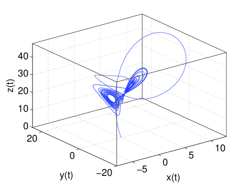
Figure 1. The fractal SL ordinary differential equations with the parameter $a=2.35$.

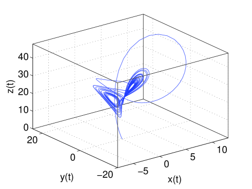
Figure 2. The fractal SL ordinary differential equations with the parameter $a=2$.

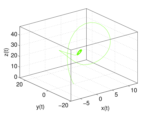
Figure 3. The fractal SL ordinary differential equations with the parameter $a=1.5$.

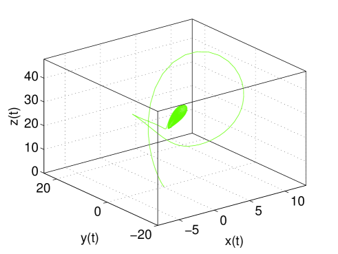
Figure 4. The fractal SL ordinary differential equations with the parameter $a=1.35$.

3. The fractal SL attractors

To present the anomalous behaviors of the fractal SL attractors, we start to observe the typical systems for the fractal SL ordinary differential equations.

3.1. The fractal SL attractor I

Making use of (10), (11), and (12) with the parameter $D=2/3$ and $\mu=0.9$, the fractal SL attractor I for the fractal SL differential equations can be presented as follows:

(13) $$\frac{10}{3}t^{\frac{2}{3}}\frac{dx\left(t\right)}{dt}=\frac{47}{20}\left({y\left(t\right)-x\left(t\right)}\right),$$

(14) $$\frac{10}{3}t^{\frac{2}{3}}\frac{dy\left(t\right)}{dt}=x\left(t\right)\left({\frac{3}{10}-z\left(t\right)}\right)-y\left(t\right),$$

and

(15) $$\frac{10}{3}t^{\frac{2}{3}}\frac{dz\left(t\right)}{dt}=x\left(t\right)y\left(t\right)-27z\left(t\right).$$

The chaotic trajectories of the SL attractor I with the parameters $D=2/3$ and $\mu=0.9$ are showed in Figure 5, where the initial conditions are $x\left(0\right)=0.1$, $y\left(0\right)=0.1$, and $z\left(0\right)=0.1$, and time $t$ changes from $0.1$ to $10^{6}$.

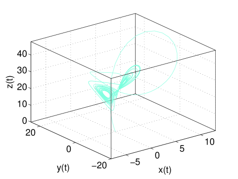
Figure 5. The fractal SL attractor I with the parameters $a=2.35$, $D=2/3$ and $\mu=0.9$.

The plane x-y of the fractal SL attractor I is shown in Figure 6, where the initial conditions are $x\left(0\right)=0.1$, $y\left(0\right)=0.1$, and $z\left(0\right)=0.1$, and time $t$ changes from $0.1$ to $10^{6}$.

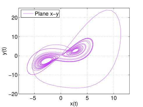
Figure 6. The plane x-y with the parameters $a=2.35$, $D=2/3$ and $\mu=0.9$.

The plane x-z of the fractal SL attractor I is given in Figure 7, where the initial conditions are $x\left(0\right)=0.1$, $y\left(0\right)=0.1$, and $z\left(0\right)=0.1$, and time $t$ changes from $0.1$ to $10^{6}$.

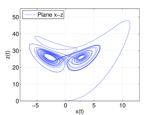
Figure 7. The plane x-z with the parameters $a=2.35$, $D=2/3$ and $\mu=0.9$.

The plane y-z of the fractal SL attractor I is depicted in Figure 8, where the initial conditions are $x\left(0\right)=0.1$, $y\left(0\right)=0.1$, and $z\left(0\right)=0.1$, and time $t$ changes from $0.1$ to $10^{6}$.

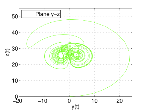
Figure 8. The plane y-z with the parameters $a=2.35$, $D=2/3$ and $\mu=0.9$.

The plots of the time series for $x\left(t\right)$, $y\left(t\right)$, and $z\left(t\right)$ are plotted in Figure 9, where $D=2/3$, $\mu=0.9$, and time $t$ changes from $0.1$ to $10^{6}$.

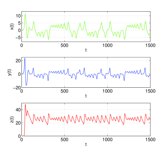
Figure 9. The time series for $x\left(t\right)$, $y\left(t\right)$, and $z\left(t\right)$ with the parameters $a=2.35$, $D=2/3$ and $\mu=0.9$.

3.2. The fractal SL attractor II

Similarly, by using (10), (11), and (12) with the parameter $D=2/3$ and $\mu=0.9$, we obtain the

(16) $$\frac{10}{3}t^{\frac{2}{3}}\frac{dx\left(t\right)}{dt}=2\left({y\left(t\right)-x\left(t\right)}\right),$$

(17) $$\frac{10}{3}t^{\frac{2}{3}}\frac{dy\left(t\right)}{dt}=x\left(t\right)\left({\frac{3}{10}-z\left(t\right)}\right)-y\left(t\right),$$

and

(18) $$\frac{10}{3}t^{\frac{2}{3}}\frac{dz\left(t\right)}{dt}=x\left(t\right)y\left(t\right)-27z\left(t\right).$$

The chaotic trajectories of the SL attractor II with the parameters $D=2/3$ and $\mu=0.9$ are showed in Figure 10, where the initial conditions are $x\left(0\right)=0.1$, $y\left(0\right)=0.1$, and $z\left(0\right)=0.1$, and time $t$ changes from $0.1$ to $10^{6}$.

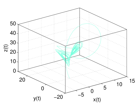
Figure 10. The fractal SL attractor II with the parameters $a=2$, $D=2/3$ and $\mu=0.9$.

The plane x-y of the fractal SL attractor II is given in Figure 11, where the initial conditions are $x\left(0\right)=0.1$, $y\left(0\right)=0.1$, and $z\left(0\right)=0.1$, and time $t$ changes from $0.1$ to $10^{6}$.

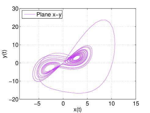
Figure 11. The plane x-y with the parameters $a=2$, $D=2/3$ and $\mu=0.9$.

The plane x-z of the fractal SL attractor II is given in Figure 12, where the initial conditions are $x\left(0\right)=0.1$, $y\left(0\right)=0.1$, and $z\left(0\right)=0.1$, and time $t$ changes from $0.1$ to $10^{6}$.

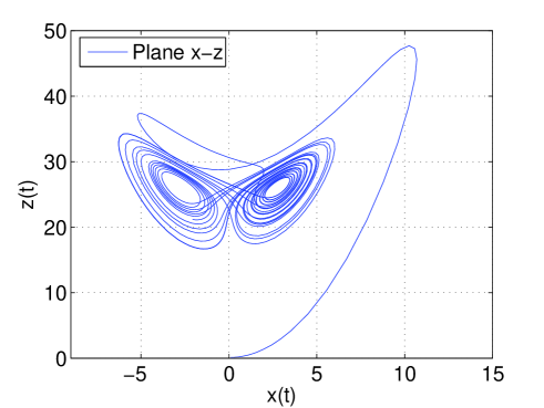
Figure 12. The plane x-z with the parameters $a=2$, $D=2/3$ and $\mu=0.9$.

The plane y-z of the fractal SL attractor II is depicted in Figure 13, where the initial conditions are $x\left(0\right)=0.1$, $y\left(0\right)=0.1$, and $z\left(0\right)=0.1$, and time $t$ changes from $0.1$ to $10^{6}$.

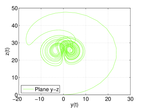
Figure 13. The plane y-z with the parameters $a=2$, $D=2/3$ and $\mu=0.9$.

The plots of the time series for $x\left(t\right)$, $y\left(t\right)$, and $z\left(t\right)$ are plotted in Figure 14, where $D=2/3$, $\mu=0.9$, and time $t$ changes from $0.1$ to $10^{6}$.

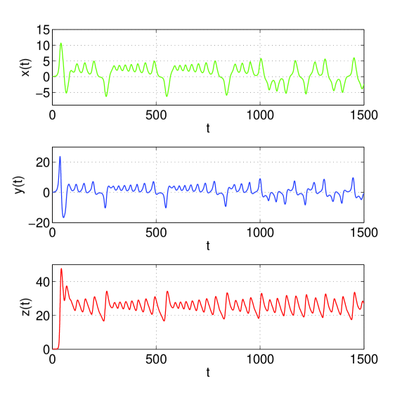
Figure 14. The time series for $x\left(t\right)$, $y\left(t\right)$, and $z\left(t\right)$ with the parameters $a=2$, $D=2/3$ and $\mu=0.9$.

4. Comparative results among the Lorenz and fractal SL attractors

To understand the anomalous behaviors of the fractal SL attractors, we compare the chaotic trajectories, phase-space parties and time series for the Lorenz and fractal SL attractors.

The chaotic trajectories for the Lorenz and fractal SL attractors is displayed in Figure 15, where the initial conditions are $x\left(0\right)=0.1$, $y\left(0\right)=0.1$, and $z\left(0\right)=0.1$.

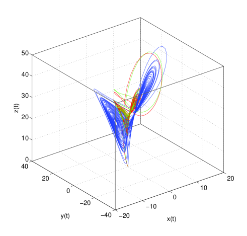
Figure 15. The chaotic trajectories for the Lorenz and fractal SL attractors. The green curve represents the chaotic trajectories for the fractal SL attractor I, where the initial conditions are $x\left(0\right)=0.1$, $y\left(0\right)=0.1$, and $z\left(0\right)=0.1$, and time $t$ changes from $0.1$ to $10^{6}$. The red curve represents the chaotic trajectories for the fractal SL attractor II, where the initial conditions are $x\left(0\right)=0.1$, $y\left(0\right)=0.1$, and $z\left(0\right)=0.1$, and time $t$ changes from $0.1$ to $10^{6}$. The blue curve represents the chaotic trajectories for the Lorenz attractor, where the initial conditions are $x\left(0\right)=0.1$, $y\left(0\right)=0.1$, and $z\left(0\right)=0.1$, and time $t$ changes from $0$ to $60$.

The plots of the plane x-y for the Lorenz and fractal SL attractors are demonstrated in Figure 16, where the initial conditions are $x\left(0\right)=0.1$, $y\left(0\right)=0.1$, and $z\left(0\right)=0.1$.

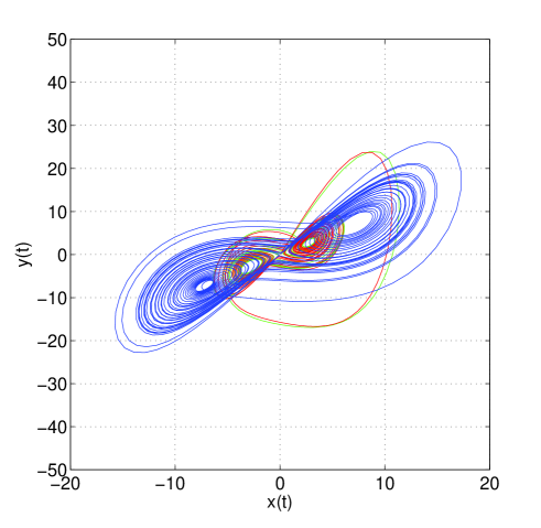
Figure 16. The plane x-y for the Lorenz and fractal SL attractors. The green curve represents the plane x-y for the fractal SL attractor I, where the initial conditions are $x\left(0\right)=0.1$, $y\left(0\right)=0.1$, and $z\left(0\right)=0.1$, and time $t$ changes from $0.1$ to $10^{6}$. The red curve represents the plane x-y for the fractal SL attractor II, where the initial conditions are $x\left(0\right)=0.1$, $y\left(0\right)=0.1$, and $z\left(0\right)=0.1$, and time $t$ changes from $0.1$ to $10^{6}$. The blue curve represents the plane x-y for the Lorenz attractor, where the initial conditions are $x\left(0\right)=0.1$, $y\left(0\right)=0.1$, and $z\left(0\right)=0.1$, and time $t$ changes from $0$ to $60$.

The plots of the plane x-z for the Lorenz and fractal SL attractors are given in Figure 17, where the initial conditions are $x\left(0\right)=0.1$, $y\left(0\right)=0.1$, and $z\left(0\right)=0.1$.

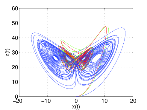
Figure 17. The plane x-z for the Lorenz and fractal SL attractors. The green curve represents the plane x-y for the fractal SL attractor I, where the initial conditions are $x\left(0\right)=0.1$, $y\left(0\right)=0.1$, and $z\left(0\right)=0.1$, and time $t$ changes from $0.1$ to $10^{6}$. The red curve represents the plane x-z for the fractal SL attractor II, where the initial conditions are $x\left(0\right)=0.1$, $y\left(0\right)=0.1$, and $z\left(0\right)=0.1$, and time $t$ changes from $0.1$ to $10^{6}$. The blue curve represents the plane x-z for the Lorenz attractor, where the initial conditions are $x\left(0\right)=0.1$, $y\left(0\right)=0.1$, and $z\left(0\right)=0.1$, and time $t$ changes from $0$ to $60$.

The plots of the plane y-z for the Lorenz and fractal SL attractors are showed in Figure 17, where the initial conditions are $x\left(0\right)=0.1$, $y\left(0\right)=0.1$, and $z\left(0\right)=0.1$.

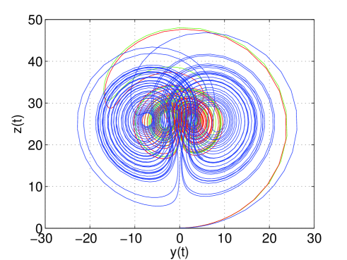
Figure 18. The plane y-z for the Lorenz and fractal SL attractors. The green curve represents the plane y-z for the fractal SL attractor I, where the initial conditions are $x\left(0\right)=0.1$, $y\left(0\right)=0.1$, and $z\left(0\right)=0.1$, and time $t$ changes from $0.1$ to $10^{6}$. The red curve represents the plane y-z for the fractal SL attractor II, where the initial conditions are $x\left(0\right)=0.1$, $y\left(0\right)=0.1$, and $z\left(0\right)=0.1$, and time $t$ changes from $0.1$ to $10^{6}$. The blue curve represents the plane y-z for the Lorenz attractor, where the initial conditions are $x\left(0\right)=0.1$, $y\left(0\right)=0.1$, and $z\left(0\right)=0.1$, and time $t$ changes from $0$ to $60$.

The plots of the time series of $x\left(t\right)$ for the Lorenz and fractal SL attractors are plotted in Figure 19, where the initial conditions are $x\left(0\right)=0.1$, $y\left(0\right)=0.1$, and $z\left(0\right)=0.1$.

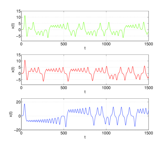
Figure 19. The time series $x\left(t\right)$ for the fractal SL and Lorenz attractors. The green curve represents the time series $x\left(t\right)$ for the fractal SL attractor I, where the initial conditions are $x\left(0\right)=0.1$, $y\left(0\right)=0.1$, and $z\left(0\right)=0.1$, and time $t$ changes from $0.1$ to $10^{6}$. The red curve represents the time series $x\left(t\right)$ for the fractal SL attractor II, where the initial conditions are $x\left(0\right)=0.1$, $y\left(0\right)=0.1$, and $z\left(0\right)=0.1$, and time $t$ changes from $0.1$ to $10^{6}$. The blue curve represents the time series $x\left(t\right)$ for the Lorenz attractor, where the initial conditions are $x\left(0\right)=0.1$, $y\left(0\right)=0.1$, and $z\left(0\right)=0.1$, and time $t$ changes from $0$ to $60$.

The plots of the time series of $x\left(t\right)$ for the Lorenz and fractal SL attractors are plotted in Figure 20, where the initial conditions are $x\left(0\right)=0.1$, $y\left(0\right)=0.1$, and $z\left(0\right)=0.1$.

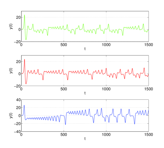
Figure 20. The time series $y\left(t\right)$ for the fractal SL and Lorenz attractors. The green curve represents the time series $y\left(t\right)$ for the fractal SL attractor I, where the initial conditions are $x\left(0\right)=0.1$, $y\left(0\right)=0.1$, and $z\left(0\right)=0.1$, and time $t$ changes from $0.1$ to $10^{6}$. The red curve represents the time series $y\left(t\right)$ for the fractal SL attractor II, where the initial conditions are $x\left(0\right)=0.1$, $y\left(0\right)=0.1$, and $z\left(0\right)=0.1$, and time $t$ changes from $0.1$ to $10^{6}$. The blue curve represents the time series $y\left(t\right)$ for the Lorenz attractor, where the initial conditions are $x\left(0\right)=0.1$, $y\left(0\right)=0.1$, and $z\left(0\right)=0.1$, and time $t$ changes from $0$ to $60$.

The plots of the time series of $z\left(t\right)$ for the Lorenz and fractal SL attractors are plotted in Figure 21, where the initial conditions are $x\left(0\right)=0.1$, $y\left(0\right)=0.1$, and $z\left(0\right)=0.1$.

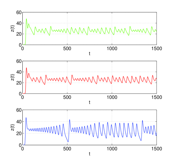
Figure 21. The time series $z\left(t\right)$ for the fractal SL and Lorenz attractors. The green curve represents the time series $y\left(t\right)$ for the fractal SL attractor I, where the initial conditions are $x\left(0\right)=0.1$, $y\left(0\right)=0.1$, and $z\left(0\right)=0.1$, and time $t$ changes from $0.1$ to $10^{6}$. The red curve represents the time series $z\left(t\right)$ for the fractal SL attractor II, where the initial conditions are $x\left(0\right)=0.1$, $y\left(0\right)=0.1$, and $z\left(0\right)=0.1$, and time $t$ changes from $0.1$ to $10^{6}$. The blue curve represents the time series $z\left(t\right)$ for the Lorenz attractor, where the initial conditions are $x\left(0\right)=0.1$, $y\left(0\right)=0.1$, and $z\left(0\right)=0.1$, and time $t$ changes from $0$ to $60$.

It is observed that the plots of the plane x-y for the fractal SL attractors show the ”Wukong effect” (see Figures 6 and 11) because they look like the face of ”Wukong” who is from the famous Chinese classical literary work The Journey to the West [15].

Let

(19) $${\rm{\bf X}}=\left({{\begin{array}[]{*{20}c}{-2\hfill}&2\hfill&0\hfill\\ {\frac{3}{10}-z\left(t\right)\hfill}&{-1\hfill}&{-x\left(t\right)\hfill}\\ {y\left(t\right)\hfill}&{x\left(t\right)\hfill}&{-27\hfill}\\ \end{array}}}\right)$$

and

(20) $${\rm{\bf\Xi}}\left(t\right)=\left({x\left(t\right),y\left(t\right),z\left(t\right)}\right).$$

The SL system of the SL ordinary differential equations (16), (17) and (18) can be rewritten as

(21) $$\frac{10}{3}t^{\frac{2}{3}}\frac{d{\rm{\bf\Xi}}\left(t\right)}{dt}={\rm{\bf X\Xi}}\left(t\right),$$

where

(22) $${\rm{\bf\Xi}}\left(0\right)=\left({x\left(0\right),y\left(0\right),z\left(0\right)}\right)$$

Thus, we have the following conjecture:

Conjecture

The chaotic system (21) with the initial condition (22) has at lest one fixed point.

5. Conclusion and Future Work

In the present work we have discovered that the SL systems exhibit the chaotic behaviors for the parameters $a=2$, $D=2/3$, and $\mu=0.9$. The SL ordinary differential equations were obtained based on the fractal SL derivative involving the Mandelbrot scaling law. By the comparison among the Lorenz and scaling-law attractors, it is seen that the fractal SL attractor shows the ”Wukong effect” whilst the Lorenz attractor shows the ”Butterfly effect”. We proposed the conjecture for the fixed point theory for the fractal SL attractor. They are nonlinear, non-periodic, three-dimensional and deterministic systems In the future, we plan to investigate the fractal dimensions and fixed point theory of the SL attractors. The mathematical structure and applications of the fractal SL system are also open problems in the study of the SL chaos theory via the fractal SL calculus.

References

- [1] Lorenz, E. N. (1963). Deterministic nonperiodic flow. Journal of Atmospheric Sciences, 20(2), 130-141.
- [2] Haken, H. (1975). Analogy between higher instabilities in fluids and lasers. Physics Letters A, 53(1), 77-78.
- [3] Knobloch, E. (1981). Chaos in the segmented disc dynamo. Physics Letters A, 82(9), 439-440.
- [4] Gorman, M., Widmann, P. J., Robbins, K. A. (1986). Nonlinear dynamics of a convection loop: a quantitative comparison of experiment with theory. Physica D: Nonlinear Phenomena, 19(2), 255-267.
- [5] Hemati, N. (1994). Strange attractors in brushless DC motors. IEEE Transactions on Circuits and Systems I: Fundamental Theory and Applications, 41(1), 40-45.
- [6] Cuomo, K. M., Oppenheim, A. V. (1993). Circuit implementation of synchronized chaos with applications to communications. Physical review letters, 71(1), 65-68.
- [7] Poland, D. (1993). Cooperative catalysis and chemical chaos: a chemical model for the Lorenz equations. Physica D: Nonlinear Phenomena, 65(1-2), 86-99.
- [8] Kolá M., Gumbs, G. (1992). Theory for the experimental observation of chaos in a rotating waterwheel. Physical review A, 45(2), 626–637.
- [9] Mishra, A. A., Sanghi, S. (2006). A study of the asymmetric Malkus waterwheel: The biased Lorenz equations. Chaos: An Interdisciplinary Journal of Nonlinear Science, 16(1), 013114.
- [10] Yang, X. J. (2020). On traveling-wave solutions for the scaling-law telegraph equations. Therm Science, 24(6B):3861–3868.
- [11] Yang, X. J., Liu, J. G., Abdel-Aty, M. On the theory of the fractal scaling-law elasticity. Meccanica (2021). https://doi.org/10.1007/s11012-021-01405-4.
- [12] Yang, X. J., Liu, J. G. (2021). A new insight to the scaling-law fluid associated with the Mandelbrot scaling law. Therm Science, 25(6B): 4561–4568.
- [13] Yang, X. J., Cui, P., Liu, J. G. (2021). A new viewpoint on theory of the scaling-law heat conduction process. Therm Science, 25(6B): 4505–4513.
- [14] Mandelbrot, B. (1967). How long is the coast of Britain? Statistical self-similarity and fractional dimension. Science, 156(3775), 636-638.
- [15] Wu, C. E. (2011). The Journey to the West. University of Chicago Press, London, Translated and Edited by Anthony C. Yu.