A sample size heuristic for network scale-up studies

Abstract

The network scale-up method (NSUM) is a survey-based method for estimating the number of individuals in a hidden or hard-to-reach subgroup of a general population. In NSUM surveys, sampled individuals report how many others they know in the subpopulation of interest (e.g. “How many sex workers do you know?”) and how many others they know in subpopulations of the general population (e.g. “How many bus drivers do you know?”). NSUM is widely used to estimate the size of important epidemiological risk groups, including men who have sex with men, sex workers, HIV+ individuals, and drug users. Unlike several other methods for population size estimation, NSUM requires only a single random sample and the estimator has a conveniently simple form. Despite its popularity, there are no published guidelines for the minimum sample size calculation to achieve a desired statistical precision. Here, we provide a sample size formula that can be employed in any NSUM survey. We show analytically and by simulation that the sample size controls error at the nominal rate and is robust to some forms of network model mis-specification. We apply this methodology to study the minimum sample size and relative error properties of several published NSUM surveys.
Keywords: network scale-up method, study design, sample size, relative error, hidden population

Abbreviations: AIDS: acquired immunodeficiency syndrome; ER: Erdős-Rényi; ERGM: exponential random graph model; FSW: female sex workers; G-NSUM: generalized NSUM; HIV: human immunodeficiency virus; MMT: methadone maintenance therapy; MSM: men who have sex with men; NSUM: network scale-up method; PA: preferential attachment; SBM: stochastic block model

1 Introduction

Estimating the size of a hidden or hard-to-reach population is an important problem in demography, epidemiology, and public health research [1]. Traditional methods, such as capture-recapture [2, 3, 4, 5, 6, 7, 8, 9, 10] and benchmark multiplier methods [11, 7, 12, 13] require multiple independent samples, but it can be costly to obtain multiple samples and difficult to guarantee that samples collected under different designs are independent [14]. Bernard et al. [15] introduced the network scale-up method (NSUM) to estimate the number of people who died in the 1985 Mexico City earthquake. NSUM has subsequently been employed to estimate the number of men who have sex with men [16, 17, 18, 19], sex workers [20, 21, 22, 19], trafficked persons [23], infected or at-risk individuals [24, 25, 26, 27, 28, 29, 19, 30, 31, 32, 33, 34, 35], drug users [36, 37, 38, 19, 20], prisoners [39], victims of disasters [40], abortions [41], choking incidents in children [42], religious individuals [43], and people in one’s personal network [44, 45].

As Maltiel et al. [46] summarized, “NSUM is based on the idea that for all individuals, the probability of knowing someone in a given subpopulation is the size of that subpopulation divided by the overall population size.” In the basic NSUM [47, 48, 49, 50], investigators obtain a single random sample of individuals in the general population, who are not necessarily members of the hidden population. Each respondent reports the number of others they know in the general population (or the number they know in several subgroups of the general population so that the number of others they know in the general population may be estimated) and also the number they know in the target population. The ratio of these average counts is multiplied by the known size of the general population to estimate the size of the target population.

Population size estimation using NSUM relies on several assumptions related to homogeneity of the underlying network of acquaintanceships and the accuracy of reported counts. Several variants and generalizations of NSUM extend the method to accommodate more flexible assumptions using complex estimators. For example, McCormick and Zheng [51] provide an adjustment for recall bias, in which the number of contacts is underestimated in large groups and overestimated in small groups. Habecker et al. [52] and Feehan and Salganik [53] formalize the incorporation of unequal sampling weights for surveyed individuals into NSUM. Maltiel et al. [46] propose a Bayesian approach that models recall bias, transmission error, and barrier effects directly. Feehan and Salganik [53] introduce a method that generalizes NSUM (called G-NSUM) by recognizing that in an undirected network, total in-degrees and out-degrees must be equal, a fact that can be exploited when two samples are obtainable. The G-NSUM was further generalized for venue-based sampling [54]. While these methods offer improved and more efficient estimates, the classic NSUM method remains widely used due to its simplicity.

As NSUM surveys grow in popularity, practitioners need guidance on how to design NSUM studies to achieve accurate and reliable results. Researchers have noted that population-size estimates from NSUM can have high variance [47, 20, 44, 27]. This may be due in part to the lack of a coherent framework that guides investigators in choosing a sample size for empirical studies. To address this gap, we present a sample size heuristic that enables researchers to calculate the number of respondents needed to estimate the size of a hidden population at a given relative error. We investigate the properties of the sample size heuristic and analyze its performance under network model mis-specificiation. Finally, we perform a retrospective sample size analysis for several existing NSUM studies and conclude with recommendations for empirical NSUM study design.

2 Setting and NSUM estimator

Consider a set $V$ of individuals of known size $M=|V|$ called the general population. A subset of individuals $U\subset V$ of size $N=|U|$ comprise the hidden population; we wish to estimate $N$. NSUM relies on information about the network of relationships between individuals. The meaning of these relationships varies according to the type of study, but may include social, epidemiological, or communication relationships. Let $G=(V,~{}E)$ represent the general population network, where $V$ is the set of individuals in the general population and $E$ is the set of relevant relationships between population members. We assume $G$ is undirected and simple, that is, contains no parallel edges or self-loops. Then for all $i,j\in V$, we have $(i,j)\in E$ whenever $i$ and $j$ share the relationship of interest. Next, define $d_{i}^{u}=|\{(j,i)\in E,~{}j\in U\}|$ to be the number of connections to the hidden population of person $i$, that is, the number of links between person $i$ and members of the hidden population $U$. Finally, define the personal network size of person $i$ – which is also called $i$’s degree – as $d_{i}=|\{(j,i)\in E,~{}j\in V\}|$, the number of edges incident to person $i$ in $G$. For simplicity, we assume below that $d_{i}$ is directly observed, but in practice NSUM studies often estimate $d_{i}$ using the known population method [25, 24] or the summation method [55].

The statistical performance of the NSUM estimator relies on assumptions about the distribution of personal network sizes $d_{i}$ and reported connections to the hidden population $d_{i}^{u}$ that imply certain global features of the underlying general population network. In many cases, these assumptions correspond to a particular random graph model. Laga et al. [49] provides a summary of network distributional assumptions in the NSUM literature. In what follows, we assume the general population network has Erdős-Rényi distribution [56]. This framework can be extended to any vertex-exchangeable graph model [57], and we illustrate in Section 4.1, with details in Appendix C, that the sample size heuristic is robust to violations of vertex-exchangeability.

Under an Erdős-Rényi model for the network $G$, edge relationships exist between individuals in $V$, and between individuals in $V$ and $U$, with probability $p$ independently of other relationships. Consequently, the following marginal degree models for person $i$ hold:

$$\begin{split}d_{i}&\sim\text{Binomial}(M-1,~{}p)\\ d_{i}^{u}&\sim\text{Binomial}(N,~{}p)\enskip.\end{split}$$ (1)

It follows that

$$\begin{split}\mathbb{E}[d_{i}]&=(M-1)p\approx Mp\\ \mathbb{E}[d_{i}^{u}]&=Np\enskip.\end{split}$$

If $i$ is a member of the target population, then $d_{i}^{u}\sim\text{Binomial}(N-1,~{}p)$ and $\mathbb{E}[d_{i}^{u}]=(N-1)p\approx Np$.

Solving for $p$ gives

$$p\approx\mathbb{E}[d_{i}^{u}]~{}/~{}N=\mathbb{E}[d_{i}]~{}/~{}M\enskip.$$ (2)

This yields an immediate formula for $N$ in terms of the expected general and hidden population degrees:

$$N\approx M\cdot\mathbb{E}[d_{i}^{u}]~{}/~{}\mathbb{E}[d_{i}]\enskip.$$ (3)

To estimate the hidden population size $N$, consider a random sample of $n$ individuals from $V$, each of whom reports how many individuals they know in different subgroups of the general population (which allows us to estimate $d_{i}$) and how many individuals they know in the hidden population (which is $d_{i}^{u}$). Using this information, NSUM estimates both of the expectations in (3) empirically by averages. Then a method of moments equation for (2) is

$$N\cdot\frac{1}{n}\sum_{i=1}^{n}d_{i}=M\cdot\frac{1}{n}\sum_{i=1}^{n}d_{i}^{u}.$$

Solving for $N$, we arrive at the classic NSUM estimator [24],

$$\widehat{N}=M\cdot\frac{\sum_{i=1}^{n}d_{i}^{u}}{\sum_{i=1}^{n}d_{i}}\enskip.$$ (4)

3 Sample size heuristic

Investigators conducting an NSUM survey must determine the minimum number of samples to collect in order to obtain a suitably precise estimate of the hidden population size $N$. To do this, investigators must first specify how precise they want their estimates to be. This means choosing a value for two parameters: (i) the confidence level, $1-\alpha$; and (ii) the relative margin of error, $\varepsilon$. In many applied studies, researchers choose to use 95% confidence intervals to express sampling uncertainty in their estimates, meaning that $\alpha=0.05$. The relative margin of error, $\varepsilon$, describes how close, in relative terms, the estimate is expected to be to the population value [58]. For example, a relative margin of error of 10% ($\varepsilon=0.1$) and a confidence level of 95% ($\alpha=0.05$) means that researchers want a sample size that produces estimates within 10% of the true value at least 95% of the time (that is, in at least 95% of repeated samples).

Formally, the minimum sample size is the smallest $n$ such that

$$\Pr\left(\frac{|\widehat{N}-N|}{N}<\varepsilon\right)\geq 1-\alpha\enskip,$$ (5)

where $|\widehat{N}-N|/N$ is the relative absolute error of the estimate. In other words, investigators seek the smallest sample size that ensures the relative error is small with high probability.

Heuristic 1.

Let the relative margin of error be $\varepsilon>0$, the confidence level be $1-\alpha$ for $0<\alpha<1$, the prevalence of the hidden population be $q=N/M$, and the average personal network size be $\overline{d}=M^{-1}\sum_{i=1}^{M}d_{i}$. The minimum sample size $n$ needed to satisfy (5) is then

$$n=\left\lceil\frac{z_{\alpha/2}^{2}}{\varepsilon^{2}}\cdot\frac{1}{q}\cdot\Big{(}\frac{1}{\overline{d}}-\frac{1}{M}\Big{)}\right\rceil\enskip,$$ (6)

where $\lceil\cdot\rceil$ is the ceiling operator and $z_{\alpha/2}$ is the $1-\alpha/2$ quantile of the standard normal distribution.

In order to use the sample size formula (6), researchers must specify the values for three population quantities: (i) the size of the general population, $M$; (ii) the prevalence of the hidden population, $q=N/M$; and (iii) the average size of respondents’ personal networks, $\overline{d}$. Several properties of the minimum sample size can be deduced immediately from (6), and these properties can be helpful in guiding the choice of these three parameters. First, when the general population size $M$ is large, the contribution of $M$ to the minimum sample size in (6) is negligible. Second, the consequences of error in estimates of $q$ and $\overline{d}$ are evident. If the prevalence of the hidden population $q$ is under-estimated, the minimum sample size increases; if $q$ is over-estimated, the minimum sample size increases. Therefore, it is preferable to over-estimate the prevalence to ensure a conservative sample size. If the average population degree $\overline{d}$ is under-estimated, the minimum sample size increases; if $\overline{d}$ is over-estimated, the minimum sample size decreases. Therefore it may be preferable for investigators seeking a conservative sample size to use an under-estimate of the average general population degree.

Figure 1, shows the relationship between prevalence and average degree in terms of the minimum sample size for a confidence level of 95% ($\alpha=0.05$), a relative margin of error of 10% ($\varepsilon=0.1$), and a general population size of $M=10,000$. For example, when $\alpha=0.05$, we have $z_{\alpha/2}\approx 2$, and thus if the relative margin of error is $\varepsilon=0.1$, the prevalence is $q=0.1$ and the average degree is $\overline{d}=10$, then the minimum sample size from (6) is approximately

$$n\approx\frac{2^{2}}{0.1^{2}}\cdot\frac{1}{0.1}\cdot\frac{1}{10}=4*100=400\enskip.$$

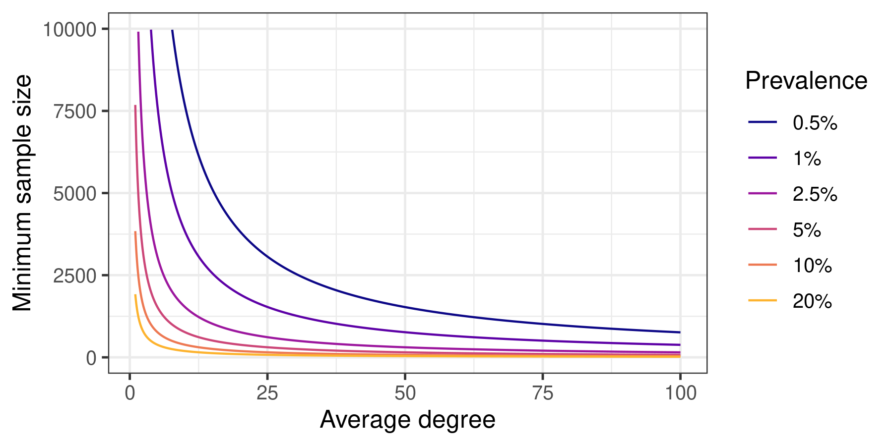
Figure 1: Sample size as a function of prevalence $(q)$ and average degree $(\overline{d})$ for $M=10,000$. We truncate the minimum sample size at the population size $M$.

Heuristic 1 is appropriate when subjects are sampled uniformly at random from the population. In practice, NSUM surveys may employ more complex sampling designs using multi-stage sampling, clustering, and stratification. These complex design features affect the variance of estimates. One common approach to modifying the sample size heuristic in (6) is through the use of a design effect for quantifying the impact of a complex sampling design on an estimate. It is defined as the ratio of the variances of an estimator with a given sampling design to a simple random sample; if $\widehat{N}_{w}$ is an NSUM estimator with a complex sampling design, then

$$D_{\textit{eff}}=\frac{\widehat{N}_{w}}{\widehat{N}}\enskip.$$ (7)

If the design effect is known a priori, then the minimum sample size calculation from Heuristic 1 can be multiplied by it to obtain an adjusted estimate.

Heuristic 2.

Let $D_{\textit{eff}}$ be the known design effect for a given sampling scheme. The minimum sample size $n$ needed to achieve (5) is approximately

$$n=\left\lceil\frac{z_{\alpha/2}^{2}}{\varepsilon^{2}}\cdot\frac{1}{q}\cdot\frac{1}{\overline{d}}\cdot D_{\textit{eff}}\right\rceil\enskip.$$ (8)

Alternatively, once a sample has been collected, an effective sample size can be computed as $n_{\textit{eff}}=~{}\frac{n}{D_{\textit{eff}}}$.

4 Results

4.1 Simulation studies

We first assess the relative error and coverage rates using the minimum sample size by simulation. We employ a factorial design that varies the population size, the prevalence, the nominal levels, and the underlying population graph model. We include i) an Erdős-Rényi network [56], ii) an exponential random graph [59], iii) a preferential attachment network [60], iv) a stochastic block model [61], and v) a small-world network [62]. Each graph model has the same expected density around $10\%$, which allows us to isolate the effect of the graph topology and assess the robustness to network model mis-specification, i.e. how well our minimum sample size calculation works when the underlying population graph implies degree models that violate (1).

The details and results are left to Appendix 4.1, but the conclusions are as follows. The average relative error is below the tolerated level $\varepsilon$ for all values of $M$ and $q$ when the underlying graph model is ER, ERGM, and small-world. For low prevalence, PA and SBM have average relative errors that exceed the tolerance level, but this is mitigated as prevalence and population size increase. Similarly, the average coverage is conservative for ER, ERGM, and small-world across different nominal levels $\alpha$, whereas it suffers for small populations with low prevalence for PA and SBM. As expected, the error bars are larger for larger values of $\alpha$. Finally, the relative error and coverage drift smoothly away from the desired levels as the underlying graph model deviates from the assumption of vertex-exchangeability.

4.2 Case studies

We now conduct a retrospective sample size analysis of published empirical NSUM surveys. Each published study reports the population size $M$, the sample size $n$ employed in the study, and the population size estimate $\widehat{N}$. To derive information about the marginal degree model, we assume that the degree reports $d_{i}$ and $d_{i}^{u}$ follow (1),

$$\begin{split}d_{i}&\sim\text{Binomial}(M,~{}\hat{d}_{i}/M)\\ d_{i}^{u}&\sim\text{Binomial}(\widehat{N},~{}\hat{d}_{i}^{u}/\widehat{N})\enskip,\end{split}$$ (9)

where $\hat{d}_{i}$, $\hat{d}_{i}^{u}$, and $\widehat{N}$ are the estimates from the study. In other words, we take the published estimate $\widehat{N}$ as the true hidden population size $N$. From this information, we calculate the minimum sample sizes $n$ according to (6) using the implied average population degree and prevalence given the published value of the general population size $M$. We use a relative error tolerance of 10% ($\varepsilon=0.1$) and 95% confidence level ($\alpha=0.05$).

Using these parameters, we compute 10,000 Monte Carlo NSUM estimates of the target population size. That is, in each replicate, we sample $n$ degree reports $d_{1},\ldots,d_{n}$ and $d_{1}^{u},\ldots,d_{n}^{u}$ following the Binomial models in (9), and use them to calculate the NSUM estimate of $N$. For each replicate, we compute the relative error of our NSUM estimate compared to the published estimate in the study, and report the Monte Carlo average relative error over all 10,000 replicates, which we denote RelErr. We apply this retrospective sample size calculation to seven published NSUM studies.

First, we revisit a study by Killworth et al. [24] to estimate the number of HIV+ individuals in 1994 in the US, around the height of the AIDS crisis. Using a telephone survey, the authors randomly sampled $n=1,554$ members of the US population. Despite the above-average response rate, the authors recognized the potential for some non-response bias. However, they do not discuss why this sample size was chosen, but they report that the survey cost $6.50 per respondent and took 10 minutes to conduct, which suggests there may have been resource constraints. One of the major contributions of this study is an improved technique for estimating personal network sizes, along with one of the first reports of the distribution of network sizes for a random sample of the US population. Using these estimates, the authors concluded that a 95% confidence interval for the number of HIV+ individuals was $\hat{N}=800,000\pm 43,000$, which was in line with estimates from the CDC on seroprevalence.

Second, we look at two applications of NSUM to estimate the number of sex workers in China [19, 22]. Chongqing, the largest province in China, had its first reported HIV case in 1993. By 2011, there were nearly 12,000 reported cases, yet population estimates of key affected populations were then unknown. Citing the need for targeted interventions and resource allocation, Guo et al. [19] employed a multistage random sample of 2,957 individuals in order to obtain NSUM estimates of key populations including female sex workers (FSW). Using their survey results, the authors estimated $\overline{d}=311$, which had not previously been estimated in Chongqing. This led to a 95% confidence interval of $\hat{N}=31,576\pm 1,980$ for the number of FSW. They also found that sex workers have a high respect factor, but, while they argue that this suggests their NSUM estimates are less likely to be underestimated, their estimate when adjusting for respect factor was 10% lower. Although this is an important study, being one of the first applications of NSUM in China, the authors note several limitations that ultimately bring additional uncertainty to the conclusions.

More recently, Jing et al. [22] incorporated a randomized response technique to an NSUM survey in 2012 of 7,964 individuals in Taiyuan, China. The authors estimate the FSW population to be $\hat{N}=~{}3,866$, which was similar to the more expensive multiplier methods and consistent with previously reported estimates of sex worker prevalence in Asia. The authors argue that this demonstrates the the appropriateness of their adjusted NSUM approach.

Next, we look at two applications of NSUM to estimate the number of men who have sex with men (MSM) [16, 17]. Since 2008, the number of HIV cases in Japan has risen constantly, with 89% of new cases attributed to MSM. However, prior to 2012, the size of the MSM population in Japan had not been estimated “in a rigorous manner” [16]. To address this, Ezoe et al. [16] employed the first internet-based NSUM estimator. The authors surveyed 1,500 individuals who were registered to Intage, an internet-research agency. They estimated the MSM prevalence among the male population to be 2.87%, which was comparable to previous studies using the direct-estimation method. These results suggest that internet surveys can be combined with NSUM for an even quicker and lower-cost method, especially in stigmatized populations.

Wang et al. [17] are also interested in estimating the number of MSM, but in Shanghai, China. Instead of an internet-based survey, the authors conducted a community-based survey across 19 districts in Shanghai consisting of 3,907 participants. Using NSUM, the authors report a 95% confidence interval for $\hat{N}$ as $36,354\pm 7,865$, but they note that “we did not take the sample design into consideration when performing variance estimation.”

Finally, we consider two applications of NSUM to quantify drug use [52, 33]. In the first, Heydari et al. [33] are interested in estimating the number of individuals using methadone maintenance therapy (MMT) in Kerman, Iran. Such data, which was previously not available, is needed to assess the effectiveness of MMT. The authors used two cross-sectional studies with multi-stage sampling to recruit 2,550 individuals. Using NSUM, they report $\hat{N}=5,289$. Furthermore, they were able to use this to estimate the treatment failure ratio, which was a novel application of NSUM and further evidence of its widespread applicability.

Similarly, Habecker et al. [52] use NSUM to estimate the number of heroin users in Nebraska in the past 30 days. In 2014, the authors received 550 completed mail surveys, which included additional questions that allowed the authors to compute and incorporate sampling weights into an improved NSUM estimator. Such improvements are particularly important when knowledge of the scope of the problem is time-sensitive. Ultimately, this yielded an estimate of a 95% confidence interval of $\hat{N}=368\pm 89$ for the number of heroin users in the past 30 days, which may be a proxy for the number of current heroin users.

Hidden population	$n$	$M$	$\widehat{N}$	$\overline{d}_{i}$	$\overline{d}_{i}^{u}$	RelErr	$n_{\textit{min}}$
Heroin users in Nebraska [52]	550	1,879,321	368	604	0.118	0.02	3,383
FSW in Taiyuan, China [22]	7,964	3,454,927	3,866	137	0.15	0.03	2,610
MMT users in Kerman, Iran [33]	2,550	611,401	5,289	235	2.03	0.01	197
FSW in Chongqing, China [19]	2,957	28,000,000	31,576	311	0.077	0.78	1,141
MSM in Shanghai, China [17]	3,907	24,000,000	36,354	236	0.159	0.56	1,119
HIV+ individuals in US [24]	1,554	250,000,000	800,000	286	0.91	0.02	438
MSM in Japan [16]	1,500	62,348,977	1,789,416	174	5.09	0.02	81

Table 1: Retrospective analysis for average relative error over 10,000 Monte Carlo estimates and minimum sample sizes from (6). The population size and average degrees are estimates from the given NSUM study.

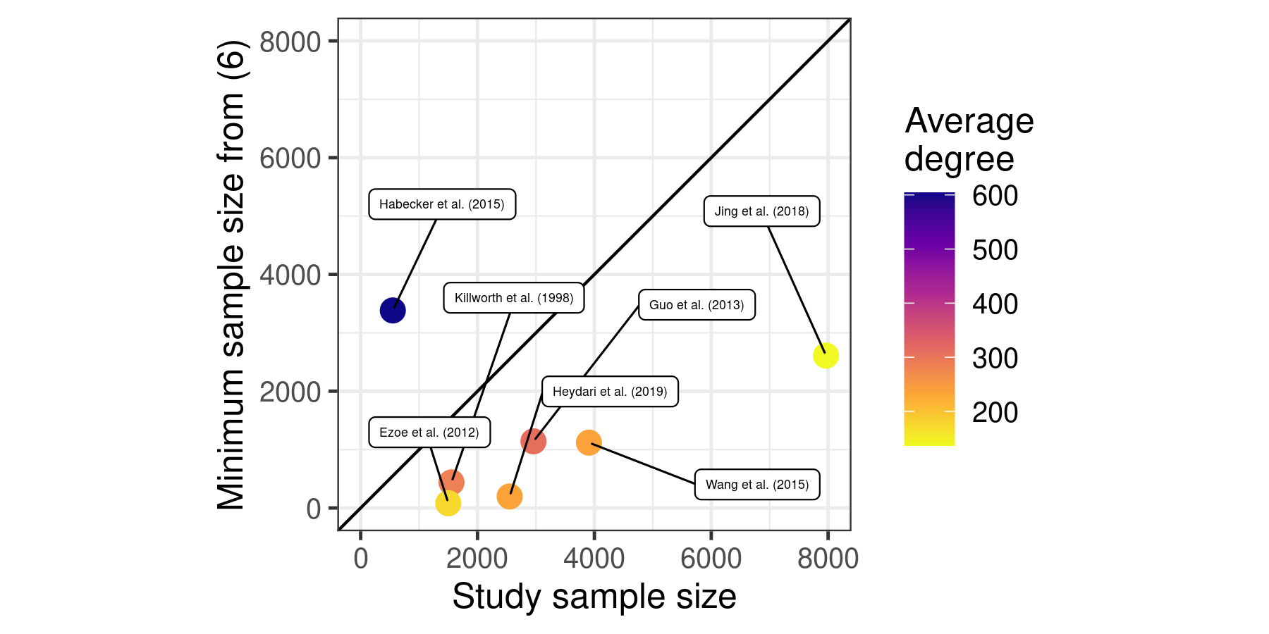
Figure 2: Study sample size compared to the minimum sample size from (6) calculated based on each study’s reported estimates of prevalence and average network size. Most of the points lie below the line $y=x$, suggesting that the actual sample size was larger than necessary to achieve 10% precision with 95% confidence.

Table 1 shows the results of the retrospective analysis on these seven studies. Figure 2 compares the actual study sample sizes and the retrospectively calculated minimum sample sizes using (6). While most of the studies have an average relative error below $0.05$, Guo et al. [19] and Wang et al. [17] may have much larger relative errors. In both of these cases, the study sample size is larger than our minimum sample size, but the average hidden population degree is much smaller than the average general population degree times the prevalence. This suggests the topology of the hidden population network differs from that of the general population network, which was a specific limitation listed by Guo et al. [19].

5 Discussion

In this paper, we have presented a simple heuristic for the minimum sample size that controls relative error (6). The heuristic is easy to employ and theoretically justified under the assumption that the general population network follows the Erdős-Rényi random graph model. Furthermore, simulations show that the sample size heuristic is robust to a variety of deviations from this idealized setting.

We also demonstrated how published NSUM studies have sample sizes that scale similarly to this minimum sample size, though most have used a sample size larger than our retrospectively calculated minimum sample size, implying that they could have saved resources by administering surveys to fewer respondents. That said, since the minimum sample sizes are functions of the reported estimates of prevalence and average network degrees, which are all quite high, it is possible that this is a propagation of biased estimates. On the other hand, one of the studies has $n<n_{\textit{min}}$, which implies they may have low precision in their estimates of the sizes of the populations of interest. In general, practitioners appear to be intuiting our heuristic as many of the study sample sizes are on the same order of magnitude as our minimum sample sizes.

In order to use the formula (6), investigators must specify values for $M$, $q$, and $\overline{d}$. In some cases, estimates of $q$ and $\overline{d}$ may be based on the results of previous studies. But, if little existing information about the hidden population is available, our results show that it will be conservative to err on the side of assuming that the hidden population is relatively low in prevalence (low $q$) and that personal network sizes are relatively small (low $\overline{d}$).

While our heuristic should help practitioners design future NSUM studies, there are several limitations to our analysis. First, the relative error controlled for in Heuristic 1 may not provide the desired absolute precision. Second, the normal approximation of our standardized estimator $\frac{\widehat{N}-N}{\sqrt{v_{n}}}$ may be invalid for small samples. Third, sample size formula may differ for more complex sampling designs and the design effects in Heuristic 2 for adjusting the minimum sample size may be unknown. Finally, non-sampling error, for instance from imperfect reporting, may dominate statistical error leading to invalid estimates even for $n\approx M$ in some cases.

Acknowledgements

We are grateful to Si Cheng, Jinghao Sun, and Clifford Zinnes for helpful comments. This work was supported by the Eunice Kennedy Shriver National Institute of Child Health and Development (1DP2HD091799-01 and P2C HD 073964 via the Berkeley Population Center). DMF also thanks the Berkeley Center for the Economics and Demography of Aging, which is funded by the National Institute on Aging (5P30AG012839).

Appendix A Variance approximations

In order to find the smallest $n$ that satisfies (5), we first need to compute the variance of the NSUM estimator in (4). Under the marginal degree model in (1), if we assume $d_{i}$ is fixed, then we have

$$\begin{split}\text{Var}(\widehat{N})&=\frac{nM^{2}}{\left(\sum_{i=1}^{n}d_{i}\right)^{2}}\text{Var}(d_{i}^{u})\\ &=\frac{nM^{2}}{\left(\sum_{i=1}^{n}d_{i}\right)^{2}}Np(1-p)\\ &\approx\frac{nM^{2}}{(nMp)^{2}}Np(1-p)\\ &=\frac{N}{n}\frac{1-p}{p}\enskip.\end{split}$$ (10)

Although early NSUM methods similarly treated these degrees as fixed, Maltiel et al. [46] argues that they should be treated as random. We show that (10) is a good approximation of the variance even when $d_{i}$ is random. In particular, we show it is a conservative estimator, i.e. at least as big as the variance approximations under alternative degree models. To do so, we begin with a review of two methods for approximating the variance of a ratio of random variables.

A.1 Taylor expansion for moments

If $Z=f(X,Y)=X/Y$ is a random variable, then we can approximate its moments by taking the expectation of an approximation of $f$ [63]. Let $\mathbb{E}[X]=\mu_{X}$ and $\text{Var}(X)=\sigma_{X}^{2}$. Similarly, let $\mathbb{E}[Y]=\mu_{Y}$ and $\text{Var}(Y)=\sigma_{Y}^{2}$. Then the first-order approximation of the variance is

$$\text{Var}(Z)\approx\frac{\mu_{X}^{2}}{\mu_{Y}^{2}}\Big{(}\frac{\sigma_{X}^{2}}{\mu_{X}^{2}}-2\frac{\text{Cov}(X,Y)}{\mu_{X}\mu_{Y}}+\frac{\sigma_{Y}^{2}}{\mu_{Y}^{2}}\Big{)}\enskip.$$ (11)

Note that this approach exploits the linearity of expectation, but there is no guarantee that inclusion of higher moments will improve the estimates. For example, the first-order approximation of $\mathbb{E}[Z]$ is

$$\mathbb{E}[Z]\approx\mu_{X}/\mu_{Y}\enskip,$$ (12)

whereas the second-order approximation is

$$\mathbb{E}[Z]\approx\frac{\mu_{X}}{\mu_{Y}}-\frac{\text{Cov}(X,Y)}{\mu_{Y}^{2}}+\frac{\mu_{X}\sigma_{Y}^{2}}{\mu_{Y}^{3}}\enskip,$$

which, from simulation, is usually not an improvement on (12).

A.2 Variance decomposition

For a model that specifies the conditional distribution of $d_{i}^{u}~{}|~{}d_{i}$, or a marginal model whose induced conditonal model is tractable, we can use the law of total variance so that we only need to linearize $Z=1/Y$:

$$\begin{split}\text{Var}(Z)&=\mathbb{E}[\text{Var}(Z~{}|~{}Y)]+\text{Var}(\mathbb{E}[Z~{}|~{}Y])\\ &=\mathbb{E}\Big{[}\frac{\sigma_{X~{}|~{}Y}^{2}}{Y}\Big{]}+\text{Var}\Big{(}\frac{\mu_{X~{}|~{}Y}}{Y}\Big{)}\\ &\approx\frac{\mathbb{E}[\sigma_{X~{}|~{}Y}^{2}]}{\mathbb{E}Y}+\frac{\mathbb{E}[\mu_{X~{}|~{}Y}]^{2}}{\mu_{Y}^{2}}\Big{(}\frac{\text{Var}(\mu_{X~{}|~{}Y})}{\mathbb{E}[\mu_{X~{}|~{}Y}]^{2}}+\frac{\sigma_{Y}^{2}}{\mu_{Y}^{2}}\Big{)}\\ &=\frac{\mathbb{E}[\sigma_{X~{}|~{}Y}^{2}]}{\mu_{Y}}+\frac{\mu_{X}^{2}}{\mu_{Y}^{2}}\Big{(}\frac{\text{Var}(\mu_{X~{}|~{}Y})}{\mu_{X}^{2}}+\frac{\sigma_{Y}^{2}}{\mu_{Y}^{2}}\Big{)}\\ &=\frac{\mathbb{E}[\sigma_{X~{}|~{}Y}^{2}]}{\mu_{Y}}+\frac{\mu_{X}^{2}}{\mu_{Y}^{2}}\Big{(}\frac{\sigma_{X}^{2}-\mathbb{E}[\sigma_{X~{}|~{}Y}^{2}]}{\mu_{X}^{2}}+\frac{\sigma_{Y}^{2}}{\mu_{Y}^{2}}\Big{)}\enskip.\end{split}$$ (13)

A.3 Examples

One drawback of the model in (1) is that it does not guarantee that $d_{i}^{u}\leq d_{i}$. Instead, by treating $d_{i}$ as random, it can be shown [1, Supplementary] that with general population sampling (from $V\setminus U$), (1) implies

$$d_{i}^{u}~{}|~{}d_{i}\sim\text{Hypergeometric}(M-1,N,d_{i})\enskip.$$

Alternatively, a conditional degree model can be specified to ensure $d_{i}^{u}\leq d_{i}$ via

$$\begin{split}d_{i}&\sim\text{Bin}(M-1,p)\\ d_{i}^{u}~{}|~{}d_{i}&\sim\text{Bin}(d_{i},p)\enskip.\end{split}$$ (14)

Killworth et al. [24] use the following variant of (14) without specifying a model for $d_{i}$:

$$d_{i}^{u}~{}|~{}d_{i}\sim\text{Bin}(d_{i},N/M)\enskip.$$ (15)

Under (15), (4) is the MLE, which is unbiased with variance $(M-N)/\overline{d}$ [46, 1, 48].

In Table 2, we provide variance approximations under different degree models. Recall that our variance estimate in (10) under the model in (1) is

$$\text{Var}(\widehat{N})=\frac{N}{n}\frac{1-p}{p}\enskip.$$

This is always greater than the variance estimate for model (1) in the first row using linearization and they are equal as $M\to\infty$. Similarly, as $N\to M$ and $M\to\infty$, the variance estimates using the decomposition for the models in rows two and three converge to twice the estimate in (10). For these reasons, the variance in (10) is conservative.

Model	Linearize $X/Y$	Linearize $1/Y$
$d_{i}^{u}\sim\text{Binomial}(N,~{}p)$	$\frac{N}{n}\frac{1-p}{p}\Big{(}1-\frac{N}{M}\Big{)}$	$\approx\frac{N}{n}\frac{1-p}{p}\Big{(}np(M-N)+2+\frac{1}{M}+\frac{N}{M^{2}}$ )
$d_{i}^{u}~{}|~{}d_{i}\sim\text{Binomial}(d_{i},~{}p)$		$Mp(1-p)\Big{(}M+\frac{1}{n}\Big{)}$
$d_{i}^{u}~{}|~{}d_{i}\sim\text{Binomial}(N,~{}p)$		$\frac{N}{n}\frac{1-p}{p}\Big{(}1+\frac{N}{M}\Big{)}$

Table 2: Variance estimates under $d_{i}\sim\text{Bin}(M-1,p)$ under two approximations: linearizing $X/Y$, explained in Section A.1, and linearizing $1/Y$, explained in Section A.2.

Appendix B Derivation of Heuristic 1

Recall that we want to find the smallest $n$ such that

$$\Pr\left(|~{}\widehat{N}-N|~{}/N<\varepsilon\right)\geq 1-\alpha\enskip.$$ (16)

By the central limit theorem, when $n$ is large, $\widehat{N}-N$ is approximated by a mean-zero normal distribution whose variance we recall from (10) as

$$v_{n}=\frac{N}{n}\frac{1-p}{p}\enskip.$$

By symmetry, (16) becomes

$$\Pr(\widehat{N}-N<N\varepsilon)\geq 1-\alpha/2\enskip.$$

Dividing by $\sqrt{v_{n}}$, we have

$$\Pr\left(\frac{\widehat{N}-N}{\sqrt{v_{n}}}<\frac{N\varepsilon}{\sqrt{v_{n}}}\right)\geq 1-\alpha/2\enskip,$$

and thus by normality,

$$\Phi\left(\frac{N\varepsilon}{\sqrt{v_{n}}}\right)\geq 1-\alpha/2\enskip,$$

where $\Phi(\cdot)$ is the cumulative distribution function of a standard normal random variable. It follows that

$$\frac{N\varepsilon}{\sqrt{v_{n}}}\geq\Phi^{-1}(1-\alpha/2)=z_{\alpha/2}\enskip,$$

where $z_{\alpha/2}$ is the $1-\alpha/2$ quantile of the standard normal distribution. Substituting the definition of $v_{n}$, we find that

$$nN\varepsilon^{2}\frac{p}{1-p}\geq z_{\alpha/2}^{2}\enskip,$$

and therefore the minimum sample size is

$$\begin{split}n&\geq\frac{z_{\alpha/2}^{2}}{N\varepsilon^{2}}\frac{1-p}{p}\\ &=\frac{z_{\alpha/2}^{2}}{\varepsilon^{2}}\frac{1}{Np}\Big{(}1-p\cdot\frac{M}{M}\Big{)}\\ &=\frac{z_{\alpha/2}^{2}}{\varepsilon^{2}}\frac{1}{\overline{d_{u}}}\Big{(}1-\frac{\overline{d}}{M}\Big{)}\\ &=\frac{z_{\alpha/2}^{2}}{\varepsilon^{2}}\frac{1}{q\overline{d}}\Big{(}1-\frac{\overline{d}}{M}\Big{)}\\ &=\frac{z_{\alpha/2}^{2}}{\varepsilon^{2}}\frac{1}{q}\Big{(}\frac{1}{\overline{d}}-\frac{1}{M}\Big{)}\enskip.\end{split}$$

$\mathrm{\square }$

Appendix C Simulations

We assess the relative error and coverage rates using the minimum sample size, by simulation. We employ a factorial design that varies the population size ($M=1000,5000,10000$), the prevalence ($q=.01,.03,\ldots,.51$), the nominal levels ($\alpha=.01,.05,.1,.2$), and the underlying population graph model. We include i) an Erdős-Rényi network [56], $G\sim\text{ER}(M,~{}p=0.1)$, ii) an exponential random graph [59] with coefficients of $-1$ for edges and triangles, iii) a preferential attachment network [60] with power of $1.4$ and $M/20$ new edges at each step, iv) a stochastic block model [61],

$$G\sim\text{SBM}\left(M,~{}\begin{pmatrix}.18&.15&.10\\ .15&.12&.05\\ .10&.05&.02\end{pmatrix}\right)\enskip,$$

and v) a small-world network [62] with a lattice of 50. We refer to these five random graph models as ER, ERGM, PA, SBM, and small-world, respectively. Each graph model has the same expected density around $10\%$, which allows us to isolate the effect of the graph topology and assess the robustness to network model mis-specification, i.e. how well our minimum sample size calculation works when the underlying population graph implies degree models that violate (1).

Figure 3 shows the average relative error and coverage over 500 replicates. The columns represent the size of the population, $M$, and the rows represent the different (true) underlying population graph model. In the top plot, the average relative error is below the tolerated level $\varepsilon$ for all values of $M$ and $q$ when the underlying graph model is ER, ERGM, and small-world. For low prevalence, PA and SBM have average relative errors that exceed the tolerance level, but this is mitigated as prevalence and population size increase. Results are similar in the bottom plot: the average coverage is conservative for ER, ERGM, and small-world across different nominal levels $\alpha$, whereas it suffers for small populations with low prevalence for PA and SBM. As expected, the error bars are larger for larger values of $\alpha$.

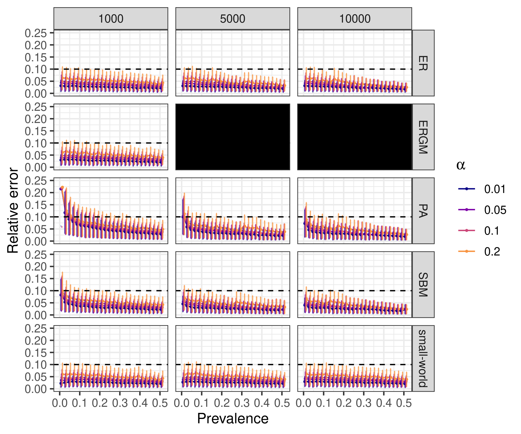
(a)

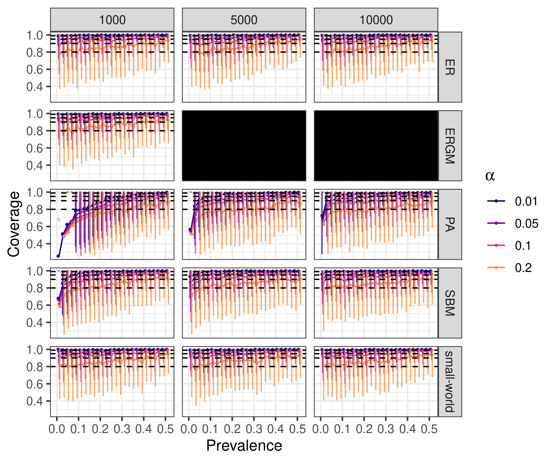
(b)

Figure 3: Relative error of $\widehat{N}$ and confidence interval coverage of the true $N$ over 500 simulated NSUM studies, as a function of prevalence $q=N/M$ and different values of the confidence level $\alpha$. (Top) Average relative error with the dashed line representing the relative error threshold $\varepsilon=0.1$. (Bottom) Average coverage with the dashed line representing the nominal levels $\alpha\in\{.01,.05,.1,.2\}$. In both plots, error bars are one standard deviation. Black panels indicate infeasibility of computation under ERGM when $M>1,000$.

Although the minimum sample size works well for all of the graph models, we would like to better understand how the performance changes as the underlying population network gradually deviates away from an Erdős-Rényi network. To do so, we consider three models. First, we have a preferential attachment (PA) network in which $M\cdot(1-\delta)$ of the nodes are an Erdős-Rényi subgraph. Second, we have a two-block stochastic block model (SBM) with $p\cdot(1+\delta)$ on the diagonal and $p\cdot(1-\delta)$ off the diagonal. Finally, we have an exponential random graph model with a triangle coefficient of $\pm\delta$, which we denote ERGM $(\pm)$. For all of these models, we vary $\delta$ from 0 to 1, and, as before, the average density for all of the networks is fixed at $10\%$. The results are shown in Figure 4. The error and coverage lie above and below, respectively, the tolerated levels only with extreme deviation from vertex-exchangeability, which further highlights the robustness of our estimator.

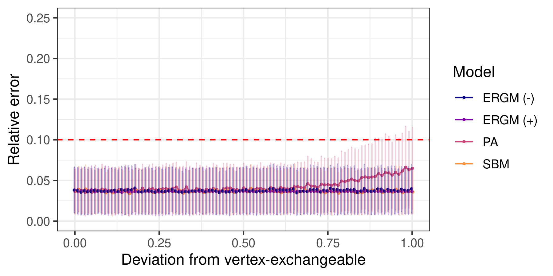
(a)

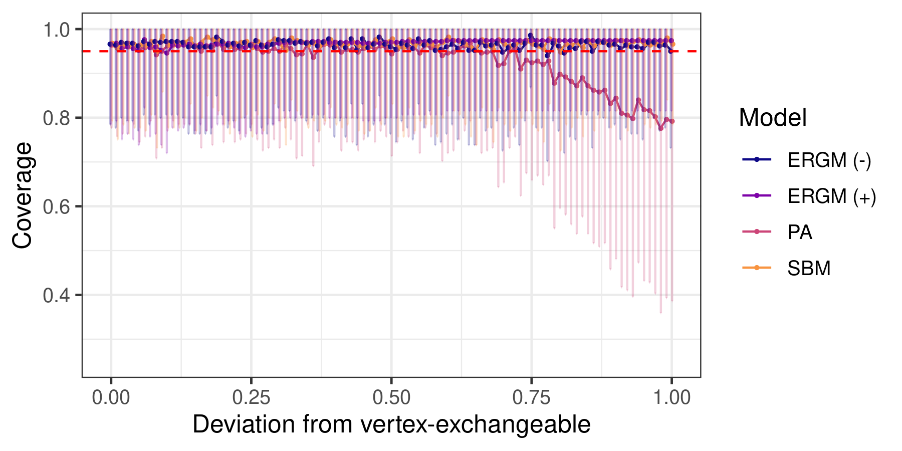
(b)

Figure 4: Relative error of $\widehat{N}$ and confidence interval coverage of the true $N$ over 500 simulated NSUM studies, by random network model. (Top) Average relative error with the dashed line representing the tolerance $\varepsilon=0.1$. (Bottom) Average coverage with the dashed line representing the nominal level $\alpha=.05$. In both plots, error bars are one standard deviation.

References

- Cheng et al. [2020] Si Cheng, Daniel J Eck, and Forrest W Crawford. Estimating the size of a hidden finite set: large-sample behavior of estimators. Statistics Surveys, 14:1–31, 2020.
- van der Heijden et al. [2015] Peter GM van der Heijden, Ieke de Vries, Dankmar Böhning, and Maarten Cruyff. Estimating the size of hard-to-reach populations using capture-recapture methodology, with a discussion of the International Labour Organization’s global estimate of forced labour. In Forum on Crime and Society, volume 8, pages 109–136. United Nations Publications, 2015.
- Karami et al. [2017] Manoochehr Karami, Salman Khazaei, Jalal Poorolajal, Alireza Soltanian, and Mansour Sajadipoor. Estimating the population size of female sex worker population in Tehran, Iran: Application of direct capture–recapture method. AIDS and Behavior, 27(8):1–7, 2017.
- Paz-Bailey et al. [2011] G Paz-Bailey, JO Jacobson, ME Guardado, FM Hernandez, AI Nieto, M Estrada, and J Creswell. How many men who have sex with men and female sex workers live in El Salvador? Using respondent-driven sampling and capture-recapture to estimate population sizes. Sexually Transmitted Infections, 87(4):279–282, 2011.
- Khan et al. [2018] Bilal Khan, Hsuan-Wei Lee, and Kirk Dombrowski. One-step estimation of networked population size with anonymity using respondent-driven capture-recapture and hashing. PLoS One, 13(4):e0195959, 2018.
- Robles et al. [1988] Sylvia C. Robles, Loraine D. Marrett, E. Aileen Clarke, and Harvey A. Risch. An application of capture-recapture methods to the estimation of completeness of cancer registration. Journal of Clinical Epidemiology, 41(5):495–501, 1988.
- Hickman et al. [2006] Matthew Hickman, Vivian Hope, Lucy Platt, Vanessa Higgins, Mark Bellis, Tim Rhodes, Colin Taylor, and Kate Tilling. Estimating prevalence of injecting drug use: A comparison of multiplier and capture–recapture methods in cities in England and Russia. Drug and Alcohol Review, 25(2):131–140, 2006.
- Bouchard [2007] Martin Bouchard. A capture-recapture model to estimate the size of criminal populations and the risks of detection in a marijuana cultivation industry. Journal of Quantitative Criminology, 23(3):221–241, 2007.
- Böhning et al. [2004] Dankmar Böhning, Busaba Suppawattanabodee, Wilai Kusolvisitkul, and Chukiat Viwatwongkasem. Estimating the number of drug users in Bangkok 2001: A capture-recapture approach using repeated entries in one list. European Journal of Epidemiology, 19(12):1075, 2004.
- Bailey [1951] Norman T. J. Bailey. On estimating the size of mobile populations from recapture data. Biometrika, 38(3/4):293–306, 1951.
- Safarnejad et al. [2017] Ali Safarnejad, Nguyen Thien Nga, and Vo Hai Son. Population size estimation of men who have sex with men in Ho Chi Minh City and Nghe An using social app multiplier method. Journal of Urban Health, 94(3):339–349, 2017.
- Zhang et al. [2007a] D. Zhang, L. Wang, F. Lv, W. Su, Y. Liu, R. Shen, and P. Bi. Advantages and challenges of using census and multiplier methods to estimate the number of female sex workers in a Chinese city. AIDS Care, 19(1):17–19, 2007a.
- Zhang et al. [2007b] Dapeng Zhang, Fan Lv, Liyan Wang, Liangxian Sun, Jian Zhou, Wenyi Su, and Peng Bi. Estimating the population of female sex workers in two Chinese cities on the basis of the HIV/AIDS behavioural surveillance approach combined with a multiplier method. Sexually Transmitted Infections, 83(3):228–231, 2007b.
- Abdul-Quader et al. [2014] Abu S. Abdul-Quader, Andrew L. Baughman, and Wolfgang Hladik. Estimating the size of key populations: Current status and future possibilities. Current Opinion in HIV and AIDS, 9(2):107–114, 2014.
- Bernard et al. [1991] H Russell Bernard, Eugene C Johnsen, Peter D Killworth, and Scott Robinson. Estimating the size of an average personal network and of an event subpopulation: Some empirical results. Social Science Research, 20(2):109–121, 1991.
- Ezoe et al. [2012] Satoshi Ezoe, Takeo Morooka, Tatsuya Noda, Miriam Lewis Sabin, and Soichi Koike. Population size estimation of men who have sex with men through the network scale-up method in Japan. PLoS One, 7(1):e31184, 2012.
- Wang et al. [2015] Jun Wang, Ying Yang, Wan Zhao, Hualin Su, Yanping Zhao, Yue Chen, Tao Zhang, and Tiejun Zhang. Application of network scale up method in the estimation of population size for men who have sex with men in Shanghai, China. PLoS One, 10(11):e0143118, 2015.
- Sulaberidze et al. [2016] Lela Sulaberidze, Ali Mirzazadeh, Ivdity Chikovani, Natia Shengelia, Nino Tsereteli, and George Gotsadze. Population size estimation of men who have sex with men in tbilisi, georgia; multiple methods and triangulation of findings. PLoS One, 11(2):e0147413, 2016.
- Guo et al. [2013] Wei Guo, Shuilian Bao, Wen Lin, Guohui Wu, Wei Zhang, Wolfgang Hladik, Abu Abdul-Quader, Marc Bulterys, Serena Fuller, and Lu Wang. Estimating the size of HIV key affected populations in Chongqing, China, using the network scale-up method. PLoS One, 8(8):e71796, 2013.
- Maghsoudi et al. [2014] Ahmad Maghsoudi, Mohammad Reza Baneshi, Mojtaba Neydavoodi, and AliAkbar Haghdoost. Network scale-up correction factors for population size estimation of people who inject drugs and female sex workers in Iran. PLoS One, 9(11):e110917, 2014.
- Jami et al. [2021] Meysam Abshenas Jami, Mohammadreza Baneshi, and Maryam Nasirian. Population size estimation of high-risk behavior in Isfahan, Iran: using the network scale-up method in 2018. Journal of Biostatistics and Epidemiology, 7(2):120–130, 2021.
- Jing et al. [2018] L Jing, Q Lu, Y Cui, H Yu, and T Wang. Combining the randomized response technique and the network scale-up method to estimate the female sex worker population size: an exploratory study. Public Health, 160:81–86, 2018.
- Shelton [2015] Janie F Shelton. Proposed utilization of the network scale-up method to estimate the prevalence of trafficked persons. In Forum on Crime and Society, volume 8, pages 85–94. United Nations Publications, 2015.
- Killworth et al. [1998a] Peter D Killworth, Christopher McCarty, H Russell Bernard, Gene Ann Shelley, and Eugene C Johnsen. Estimation of seroprevalence, rape, and homelessness in the United States using a social network approach. Evaluation Review, 22(2):289–308, 1998a.
- Killworth et al. [1998b] Peter D Killworth, Eugene C Johnsen, Christopher McCarty, Gene Ann Shelley, and H Russell Bernard. A social network approach to estimating seroprevalence in the United States. Social Networks, 20(1):23–50, 1998b.
- UNAIDS and World Health Organization [2010] UNAIDS and World Health Organization. Guidelines on estimating the size of populations most at risk to HIV. Technical report, Geneva, Switzerland, 2010. URL http://www.unaids.org/en/resources/documents/2011/2011_Estimating_Populations.
- Salganik et al. [2011] Matthew J. Salganik, Dimitri Fazito, Neilane Bertoni, Alexandre H. Abdo, Maeve B. Mello, and Francisco I. Bastos. Assessing network scale-up estimates for groups most at risk of HIV/AIDS: Evidence from a multiple-method study of heavy drug users in Curitiba, Brazil. American Journal of Epidemiology, 174(10):1190, 2011.
- Shokoohi et al. [2012] Mostafa Shokoohi, Mohammad Reza Baneshi, and Haghdoost Ali-akbar. Size estimation of groups at high risk of HIV/AIDS using network scale up in Kerman, Iran. International Journal of Preventive Medicine, 3(7), 2012.
- Center [2012] Rwanda Biomedical Center. Estimating the size of key populations at higher risk of HIV through a household survey (ESPHS). Technical report, RBC/IHDPC, SPF, UNAIDS and ICF International, Calverton, Maryland, USA, 2012.
- JafariKhounigh et al. [2014] Ali JafariKhounigh, Ali Akbar Haghdoost, Shaker SalariLak, Ali Hossein Zeinalzadeh, Reza Yousefi-Farkhad, Mehdi Mohammadzadeh, and Kourosh Holakouie-Naieni. Size estimation of most-at-risk groups of hiv/aids using network scale-up in Tabriz, Iran. Journal of Clinical Research & Governance, 3(1):21–26, 2014.
- Jing et al. [2014] Liwei Jing, Chengyi Qu, Hongmei Yu, Tong Wang, and Yuehua Cui. Estimating the sizes of populations at high risk for hiv: a comparison study. PLoS One, 9(4):e95601, 2014.
- Teo et al. [2019] Alvin Kuo Jing Teo, Kiesha Prem, Mark IC Chen, Adrian Roellin, Mee Lian Wong, Hanh Hao La, and Alex R Cook. Estimating the size of key populations for hiv in singapore using the network scale-up method. Sexually Transmitted Infections, 95(8):602–607, 2019.
- Heydari et al. [2019] Zeynab Heydari, Mohammad Reza Baneshi, Hamid Sharifi, Maryam Zamanian, Saiedeh Haji-Maghsoudi, and Farzaneh Zolala. Evaluation of the treatment failure ratio in individuals receiving methadone maintenance therapy via the network scale up method. International Journal of Drug Policy, 73:36–41, 2019.
- Haghdoost et al. [2015] Ali Akbar Haghdoost, Mohammad Reza Baneshi, Saeedeh Haji-Maghsoodi, Hossein Molavi-Vardanjani, and Elham Mohebbi. Application of a network scale-up method to estimate the size of population of breast, ovarian/cervical, prostate and bladder cancers. Asian Pacific Journal of Cancer Prevention, 16(8):3273–3277, 2015.
- Sajjadi et al. [2018] Homeira Sajjadi, Zahra Jorjoran Shushtari, Mohsen Shati, Yahya Salimi, Masoomeh Dejman, Meroe Vameghi, Salahedin Karimi, and Zohreh Mahmoodi. An indirect estimation of the population size of students with high-risk behaviors in select universities of medical sciences: A network scale-up study. PLoS One, 13(5):e0195364, 2018.
- Kadushin et al. [2006] Charles Kadushin, Peter D. Killworth, H. Russell Bernard, and Andrew A. Beveridge. Scale-up methods as applied to estimates of heroin use. Journal of Drug Issues, 36(2):417–440, 2006.
- Nikfarjam et al. [2016] Ali Nikfarjam, Mostafa Shokoohi, Armita Shahesmaeili, Ali Akbar Haghdoost, Mohammad Reza Baneshi, Saiedeh Haji-Maghsoudi, Azam Rastegari, Abbas Ali Nasehi, Nadereh Memaryan, and Termeh Tarjoman. National population size estimation of illicit drug users through the network scale-up method in 2013 in Iran. International Journal of Drug Policy, 31:147–152, 2016.
- Sheikhzadeh et al. [2016] Khodadad Sheikhzadeh, Mohammad Reza Baneshi, Mahdi Afshari, and Ali Akbar Haghdoost. Comparing direct, network scale-up, and proxy respondent methods in estimating risky behaviors among collegians. Journal of Substance Use, 21(1):9–13, 2016.
- Zheng et al. [2006] Tian Zheng, Matthew J. Salganik, and Andrew Gelman. How many people do you know in prison? Using overdispersion in count data to estimate social structure in networks. Journal of the American Statistical Association, 101(474):409–423, 2006.
- Bernard et al. [2001] H Russell Bernard, Peter D Killworth, Eugene C Johnsen, Gene A Shelley, and Christopher McCarty. Estimating the ripple effect of a disaster. Connections, 24(2):18–22, 2001.
- Rastegari et al. [2014] Azam Rastegari, Mohammad Reza Baneshi, Saiedeh Haji-Maghsoudi, Nowzar Nakhaee, Mohammad Eslami, Hossein Malekafzali, and Ali Akbar Haghdoost. Estimating the annual incidence of abortions in Iran applying a network scale-up approach. Iranian Red Crescent Medical Journal, 16(10), 2014.
- Snidero et al. [2007] Silvia Snidero, Bruno Morra, Roberto Corradetti, and Dario Gregori. Use of the scale-up methods in injury prevention research: An empirical assessment to the case of choking in children. Social Networks, 29(4):527–538, 2007.
- Yang and Yang [2017] Xiaozhao Yousef Yang and Fenggang Yang. Estimating religious populations with the network scale-up method: A practical alternative to self-report. Journal for the Scientific Study of Religion, 56(4):703–719, 2017.
- McCormick et al. [2010] Tyler H McCormick, Matthew J Salganik, and Tian Zheng. How many people do you know?: Efficiently estimating personal network size. Journal of the American Statistical Association, 105(489):59–70, 2010.
- Narouee et al. [2020] Sakineh Narouee, Mohsen Shatti, Mahnaz Didevar, and Mahshid Nasehi. Estimating social network size using network scale-up method (nsum) in Iranshahr, Sistan and Baluchestan Province, Iran. Medical journal of the Islamic Republic of Iran, 34:35, 2020.
- Maltiel et al. [2015] Rachael Maltiel, Adrian E Raftery, Tyler H McCormick, and Aaron J Baraff. Estimating population size using the network scale up method. The Annals of Applied Statistics, 9(3):1247, 2015.
- Bernard et al. [2010] H. R. Bernard, T. Hallett, A. Iovita, E. C. Johnsen, R. Lyerla, C. McCarty, M. Mahy, M. J. Salganik, T. Saliuk, O. Scutelniciuc, G. A. Shelley, P. Sirinirund, S. Weir, and D. F. Stroup. Counting hard-to-count populations: The network scale-up method for public health. Sexually Transmitted Infections, 86(Suppl 2):ii11–15, 2010.
- McCormick [2020] Tyler H McCormick. The network scale-up method. The Oxford Handbook of Social Networks, page 153, 2020.
- Laga et al. [2021] Ian Laga, Le Bao, and Xiaoyue Niu. Thirty years of the network scale-up method. Journal of the American Statistical Association, (just-accepted):1–33, 2021.
- Habecker [2017] Patrick Habecker. Who Do You Know: Improving and Exploring the Network Scale-Up Method. PhD thesis, The University of Nebraska-Lincoln, 2017.
- McCormick and Zheng [2007] Tyler H McCormick and Tian Zheng. Adjusting for recall bias in “how many x’s do you know?” surveys. In Proceedings of the Joint Statistical Meetings. Citeseer, 2007.
- Habecker et al. [2015] Patrick Habecker, Kirk Dombrowski, and Bilal Khan. Improving the network scale-up estimator: Incorporating means of sums, recursive back estimation, and sampling weights. PLoS One, 10(12):e0143406, 2015.
- Feehan and Salganik [2016] Dennis M. Feehan and Matthew J. Salganik. Estimating the size of hidden populations using the generalized network scale-up estimator. Sociological Methodology, 46(1):153–186, 2016.
- Verdery et al. [2019] Ashton M Verdery, Sharon Weir, Zahra Reynolds, Grace Mulholland, and Jessie K Edwards. Estimating hidden population sizes with venue-based sampling: Extensions of the generalized network scale-up estimator. Epidemiology (Cambridge, Mass.), 30(6):901, 2019.
- McCarty et al. [2001] Christopher McCarty, Peter D Killworth, H Russell Bernard, Eugene C Johnsen, and Gene A Shelley. Comparing two methods for estimating network size. Human organization, 60(1):28–39, 2001.
- Erdős and Rényi [1959] P Erdős and A Rényi. On random graphs I. Publicationes Mathematicae, 6:290–297, 1959.
- Diaconis and Janson [2007] Persi Diaconis and Svante Janson. Graph limits and exchangeable random graphs. arXiv preprint arXiv:0712.2749, 2007.
- Valliant et al. [2013] Richard Valliant, Jill A Dever, and Frauke Kreuter. Practical tools for designing and weighting survey samples, volume 1. Springer, 2013.
- Robins et al. [2007] Garry Robins, Pip Pattison, Yuval Kalish, and Dean Lusher. An introduction to exponential random graph (p*) models for social networks. Social networks, 29(2):173–191, 2007.
- Barabási and Albert [1999] Albert-László Barabási and Réka Albert. Emergence of scaling in random networks. Science, 286(5439):509–512, 1999.
- Holland et al. [1983] Paul W Holland, Kathryn Blackmond Laskey, and Samuel Leinhardt. Stochastic blockmodels: First steps. Social networks, 5(2):109–137, 1983.
- Watts and Strogatz [1998] Duncan J Watts and Steven H Strogatz. Collective dynamics of ‘small-world’ networks. Nature, 393(6684):440–442, 1998.
- Seltman [2012] Howard Seltman. Approximations for mean and variance of a ratio. Unpublished note, 2012.