Recurrent Variational Network: A Deep Learning Inverse Problem Solver applied to the task of Accelerated MRI Reconstruction

Abstract

Magnetic Resonance Imaging can produce detailed images of the anatomy and physiology of the human body that can assist doctors in diagnosing and treating pathologies such as tumours. However, MRI suffers from very long acquisition times that make it susceptible to patient motion artifacts and limit its potential to deliver dynamic treatments. Conventional approaches such as Parallel Imaging and Compressed Sensing allow for an increase in MRI acquisition speed by reconstructing MR images from sub-sampled MRI data acquired using multiple receiver coils. Recent advancements in Deep Learning combined with Parallel Imaging and Compressed Sensing techniques have the potential to produce high-fidelity reconstructions from highly accelerated MRI data. In this work we present a novel Deep Learning-based Inverse Problem solver applied to the task of Accelerated MRI Reconstruction, called the Recurrent Variational Network (RecurrentVarNet), by exploiting the properties of Convolutional Recurrent Neural Networks and unrolled algorithms for solving Inverse Problems. The RecurrentVarNet consists of multiple recurrent blocks, each responsible for one iteration of the unrolled variational optimization scheme for solving the inverse problem of multi-coil Accelerated MRI Reconstruction. Contrary to traditional approaches, the optimization steps are performed in the observation domain ($k$-space) instead of the image domain. Each block of the RecurrentVarNet refines the observed $k$-space and comprises a data consistency term and a recurrent unit which takes as input a learned hidden state and the prediction of the previous block. Our proposed method achieves new state of the art qualitative and quantitative reconstruction results on 5-fold and 10-fold accelerated data from a public multi-coil brain dataset, outperforming previous conventional and deep learning-based approaches. Our code is publicly available at https://github.com/NKI-AI/direct.

Keywords Accelerating MRI  $\cdot$ Deep MRI Reconstruction  $\cdot$ Inverse Problem Solvers  $\cdot$ Variational Networks  $\cdot$ Convolutional Recurrent Networks  $\cdot$ Deep Learning

1 Introduction

Figure 1: Overview of our proposed framework, Recurrent Variational Network (RecurrentVarNet), applied to the task of multi-coil Accelerated MRI Reconstruction. Our model takes as input sub-sampled MRI data from multiple coils which are refined following an iterative gradient descent-like optimization scheme of $T$ time-steps in the $k$-space, and outputs an estimate of the ground truth reconstructed image.

Magnetic Resonance Imaging (MRI) is one of the most vastly used imaging modalities in medicine. Since MRI allows for production of highly detailed anatomical images of the human body, it is often employed for disease detection, prognosis, and treatment monitoring and guidance. The facts that MRI is non-invasive and that it does not involve exposure to ionizing radiation have played a pivotal role in making it a popular imaging technique.

However, MRI is still bounded by very lengthy acquisition times induced by the fact that the MRI scanner reads data in the frequency domain ($k$-space) sequentially in time. This usually causes patient discomfort and motion artifacts, and it also limits its use for delivery of dynamic treatments such as image-guided radiotherapy. Therefore, reducing the scanning time in MRI, often referred to as accelerating MRI [1], not only could assist in reducing medical costs and patients’ distress, but could also make dynamic treatments feasible. Conventional approaches for accelerating MRI include Parallel Imaging (PI) [2, 3, 4], Compressed Sensing (CS) [5, 6], and the combination of these two methods (PI-CS) [7].

In contrast to traditional MRI acquisitions, in PI multiple, instead of one, radio-frequency receiver coils are employed to simultaneously obtain reduced sets of measurements to shorten the acquisition time. Coil sensitivity maps are required to be known since each coil is sensitive to a different part of the volume according to its position. Classical approaches for estimating these coil sensitivity maps include E-SPIRiT [8], SENSE [9, 10], GRAPPA [11], and SMASH [12].

Besides PI, CS techniques aim in accelerating the MRI acquisition by sub-sampling the $k$-space, that is, acquiring sparse or partial raw $k$-space measurements. Unfortunately, this is accompanied by a degradation of image quality, known as aliasing artifacts, which include low-resolution images, blurring, or in-folding artifacts [13]. This is attributed to the fact that this violates the Nyquist-Shannon sampling criterion [14, 15]. In CS, an acceleration factor $R$ is chosen which determines the magnitude of the acceleration, and is referred to as $R$-fold acceleration. $R$ is calculated as the ratio of the number of $k$-space measurements needed for a full scan over the number of the acquired measurements.

Recent advancements in Deep Learning (DL) and specifically in Convolutional Neural Networks (CNNs), have led to their application in many fields including solving inverse problems arising in imaging, such as Accelerated MRI Reconstruction tasks. Combined with PI-CS, DL-based methods can outperform conventional PI and CS approaches by producing reconstructed MR images with less artifacts [16]. Additionally, in 2018-19 the fastMRI [1, 17] and Calgary-Campinas [18] challenges, have provided the MRI community with publicly available raw MRI data enabling the development of multiple DL state of the art baselines for producing faithful reconstructed images from sub-sampled $k$-space measurements [19, 20, 21, 22, 23].

Motivated by the need to accelerate the MRI acquisition even further, in this work we propose a novel CNN and recurrent-based DL inverse problem solver inspired by the Variational Network [24] and the Recurrent Inference Machine [25] approaches which we apply on the task of reconstructing images from accelerated MRI data. We call our proposed method the Recurrent Variational Network.

Contributions

• We propose the Recurrent Variational Network, a novel Deep Learning architecture for solving imaging inverse problems. We applied our method to the multi-coil accelerated MRI reconstruction task.

• We are the first to present a recurrent-based DL imaging inverse problem solver that performs iterative optimization in the measurements ($k$-space) domain.

• Our quantitative and qualitative experiments demonstrate that our model achieved state of the art results on the Calgary-Campinas public brain dataset outperforming current baselines.

2 Background and Related work

2.1 MRI Acquisition

In clinical settings, the acquisition of MRI measurements by the MR scanner, also known as $k$-space, is performed in the frequency or Fourier domain. Let $n\,=\,n_{x}\times n_{y}$ denote the spatial size of the data. In the case of single-coil acquisition, the equation between the underlying spatial ground truth image $\mathbf{x}\,\in\,\mathbb{C}^{n}$ and the $k$-space $\mathbf{y}\,\in\,\mathbb{C}^{n}$ is given by

$$\mathbf{y}\,=\,\mathcal{F}(\mathbf{x})\,+\,\mathbf{e},$$ (1)

where $\mathcal{F}$ denotes the two-dimensional Fourier transform and $\mathbf{e}\,\in\,\mathbb{C}^{n}$ denotes some measurement noise, usually assumed additive and normally distributed.

2.2 Accelerated MRI Acquisition

In Parallel Imaging, multiple ($n_{c}$) receiver coils are placed around the subject to speed up the acquisition. The acquired measurements $\mathbf{y}\,=\,\{\mathbf{y}^{k}\}_{k=1}^{n_{c}}$ in the case of multi-coil acquisition can be described as

$$\mathbf{y}^{k}\,=\,\mathcal{F}(\mathbf{S}^{k}\mathbf{x})\,+\,\mathbf{e}^{k},\quad k\,=\,1,\,2,\,...,\,n_{c},$$ (2)

where $\mathbf{e}^{k}$ denotes measurement noise from the $k$-th coil and $\mathbf{S}^{k}\,\in\,\mathbb{C}^{n\times n}$ is called the sensitivity map of the $k$-th coil. The sensitivity maps encode the spatial sensitivity of their respective coil and they can be expressed with diagonal matrices. They are usually normalized such that

$$\sum_{k=1}^{n_{c}}{\mathbf{S}^{k}}^{*}{\mathbf{S}^{k}}\,=\,\mathbf{I}_{n}.$$ (3)

To accelerate the MRI acquisition, in CS settings the $k$-space is sub-sampled. The sub-sampled $k$-space measurements can be defined in terms of the fully-sampled $k$-space measurements as follows:

$$\tilde{\mathbf{y}}^{k}\,=\,\mathbf{U}\mathbf{y}^{k}\,=\,\mathbf{U}\mathcal{F}(\mathbf{S}^{k}\mathbf{x})\,+\,\tilde{\mathbf{e}}^{k},\quad k\,=\,1,\,2,\,...,\,n_{c}$$ (4)

where $\mathbf{U}\,\in\,\{0,\,1\}^{n}$ is a sub-sampling mask operator and is dependent on the acceleration factor $R$. Note that the same sub-sampling mask is applied to each coil data.

Sensitivity maps can be estimated by fully-sampling the center region of the $k$-space. This is known in the literature as the auto-calibration signal (ACS) which includes the low-frequency samples. We denote as $\mathbf{U}_{\text{ACS}}$ the ACS operator which takes as input $k$-space data and outputs the auto-calibration signal. An estimate for the sensitivity map of the $k$-th coil can be obtained as

$$\tilde{\mathbf{S}}^{k}\,=\,\mathcal{F}^{-1}(\mathbf{U}_{\text{ACS}}\tilde{\mathbf{y}}^{k})\oslash\text{RSS}\Big{(}\big{\{}\mathcal{F}^{-1}(\mathbf{U}_{\text{ACS}}\tilde{\mathbf{y}}^{l})\big{\}}_{l=1}^{n_{c}}\Big{)},$$ (5)

where $\oslash$ denotes the element-wise (Hadamard) division and $\text{RSS}:\mathbb{C}^{n\times n_{c}}\rightarrow\mathbb{R}^{n}$ the root-sum-of-squares operator [26] defined as

$$\text{RSS}(\mathbf{x}^{1}\,...,\,\mathbf{x}^{n_{c}})\,=\,\bigg{(}\sum_{k=1}^{n_{c}}|\mathbf{x}^{k}|^{2}\bigg{)}^{1/2}.$$ (6)

Note that $\mathbf{U}(\mathbf{y})\,=\,\mathbf{U}_{\text{ACS}}(\mathbf{y})$ for the samples of the ACS region.

2.3 Accelerated MRI Reconstruction as an Inverse Problem

Reconstructing MR images from sub-sampled data is an inverse problem with (4) posing as the forward model. Since (4) is ill-posed [27], an explicit solution for the image $\mathbf{x}$ is hard to obtain. In general, (4) can be treated as a variational optimization problem [24, 28], that is, solving

$$\hat{\mathbf{x}}\,=\,\arg\min_{\mathbf{z}\,\in\,\mathbb{C}^{n}}\,\sum_{k=1}^{n_{c}}\mathcal{L}\big{(}\mathbf{U}\mathcal{F}(\mathbf{S}^{k}\mathbf{z}),\,\tilde{\mathbf{y}}^{k}\big{)}\,+\,\lambda\,\mathcal{C}(\mathbf{z})$$ (7)

where $\mathcal{L}:\mathbb{C}^{n\times n_{c}}\times\mathbb{C}^{n\times n_{c}}\rightarrow\mathbb{R}^{+}$ and $\mathcal{C}:\mathbb{C}^{n}\rightarrow\mathbb{R}$ denote convex data fidelity and regularization functionals, respectively, and $\lambda\,>\,0$ the regularization parameter.

By defining an expand operator $\mathcal{E}:\mathbb{C}^{n}\times\mathbb{C}^{n\times n_{c}}\rightarrow\mathbb{C}^{n\times n_{c}}$ that takes as input an image and outputs the individual coil images and a reduce operator $\mathcal{R}:\mathbb{C}^{n\times n_{c}}\times\mathbb{C}^{n\times n_{c}}\rightarrow\mathbb{C}^{n}$ that combines the individual coil images into one image as

$$\begin{gathered}\mathcal{E}(\mathbf{z})\,=\,(\mathbf{S}^{1}\mathbf{z},\,...,\,\mathbf{S}^{n_{c}}\mathbf{z})\,=\,(\mathbf{z}^{1},\,...,\,\mathbf{z}^{n_{c}})\\ \mathcal{R}(\mathbf{z}^{1},\,...,\,\mathbf{z}^{n_{c}})\,=\,\sum_{k=1}^{n_{c}}{\mathbf{S}^{k}}^{*}\mathbf{z}^{k},\end{gathered}$$ (8)

we can define as the linear forward operator of multi-coil accelerated MRI reconstruction $\mathcal{A}:\mathbb{C}^{n}\rightarrow\mathbb{C}^{n\times n_{c}}$ and its adjoint (backward) operator $\mathcal{A}^{*}:\mathbb{C}^{n\times n_{c}}\rightarrow\mathbb{C}^{n}$ as composition of operators:

$$\mathcal{A}\,=\,\mathbf{U}\,\circ\,\mathcal{F}\,\circ\,\mathcal{E},\quad\mathcal{A}^{*}\,=\,\mathcal{R}\,\circ\,\mathcal{F}^{-1}\,\circ\,\mathbf{U},$$ (9)

where $\mathcal{F}$, $\mathcal{F}^{-1}$ and $\mathbf{U}$ are applied element-wise.

Let $\tilde{\mathbf{y}}\,=\,(\tilde{\mathbf{y}}^{1},\,...,\,\tilde{\mathbf{y}}^{n_{c}})$, then, we can define (7) in a more compact notation:

$$\hat{\mathbf{x}}\,=\,\arg\min_{\mathbf{z}\,\in\,\mathbb{C}^{n}}\,\mathcal{L}\big{(}\mathcal{A}(\mathbf{z}),\,\tilde{\mathbf{y}}\big{)}\,+\,\lambda\,\mathcal{C}(\mathbf{z}).$$ (10)

Note that the operators $\mathcal{E}$ and $\mathcal{R}$ take also as inputs the coil sensitivity maps which we omit to save space.

In this work we solve a regularised least-squares variational problem, that is, replacing $\mathcal{L}$ in (10) with the squared $\mathcal{L}_{2}$-norm:

$$\hat{\mathbf{x}}\,=\,\arg\min_{\mathbf{z}\,\in\,\mathbb{C}^{n}}\,\frac{1}{2}\,||\mathcal{A}(\mathbf{z})\,-\,\tilde{\mathbf{y}}||_{2}^{2}\,+\,\lambda\,\mathcal{C}(\mathbf{z}).$$ (11)

An approximate solution to (11) can be acquired by unrolling a gradient descent scheme [24] solved over $T$ iterations

$$\mathbf{z}_{t+1}\,=\,\mathbf{z}_{t}\,-\,\alpha_{t+1}\,\bigg{(}\mathcal{A}^{*}\big{(}\mathcal{A}(\mathbf{z}_{t})\,-\,\tilde{\mathbf{y}}\big{)}\,+\,\lambda\,\mathbf{\nabla}\mathcal{C}(\mathbf{z}_{t})\bigg{)}$$ (12)

where $t\,=\,0,\,1,\,...,\,T\,-\,1$, and $\alpha_{t+1}\,>\,0$ is the step-size at iteration $t$ and $\mathbf{z}_{0}$ is a suitable initial guess.

2.4 Deep Accelerated MRI Reconstruction

With the advent of the involvement of Deep Learning in accelerated MRI reconstruction tasks, a plethora of algorithms have been deployed with some reaching state of the art performance [17, 18]. These methods can be divided into three sub-groups:

• Image domain-learning models which operate exclusively in the image domain [24, 1, 23, 22].

• $k$-space domain-learning models which operate exclusively in the $k$-space domain [29, 30, 31].

• Hybrid (image and $k$-space) domain-learning models which alternate between image and $k$-space domains [32, 33, 19, 20, 21].

In this paper we base our work on two approaches: the End-to-End Variational Network (E2EVarNet) [21] and the Recurrent Inference Machine (RIM) [25, 22]. The former is a hybrid domain-learning model which builds upon Variational Networks [24] by using a CNN-based neural network in the image domain to perform an iterative optimization scheme in the $k$-space domain by adapting (11). The latter, is an image domain-learning model that solves (11) by treating it as a maximum-a-posteriori (MAP) estimation problem [28]. By employing a sequence of alternating CNNs and Convolutional Gated Recurrent Units (ConvGRUs), RIM learns to predict an incremental update after each iteration using as inputs the previous image prediction, a hidden state, and the gradient of the negative log-likelihood distribution.

In Sec. 3 we extensively describe the architecture of our proposed method which is a hybrid domain-learning model, as it performs optimization in the measurements ($k$-space) domain using a recurrent CNN-based network which, however, operates in the image domain.

3 Method

In this work we introduce the Recurrent Variational Network (RecurrentVarNet), which is an end-to-end inverse problem solver framework that performs a gradient descent-like optimization in the measurements domain using convolutional recurrent neural networks. In this paper we particularized RecurrentVarNet to the task of Accelerated MRI Reconstruction following the next steps:

First, we replaced the need of explicitly defining a regularization term $\mathcal{C}$ in (11) and computing its gradient in (12) with a CNN-based image-refinement model $\mathcal{G}_{\theta_{t+1}}$ at each layer $t\,=\,0,\,1,\,...,\,T\,-\,1$:

$$\mathbf{z}_{t+1}\,=\,\mathbf{z}_{t}\,-\,\alpha_{t+1}\,\mathcal{A}^{*}\big{(}\mathcal{A}(\mathbf{z}_{t})\,-\,\tilde{\mathbf{y}}\big{)}\,+\,\mathcal{G}_{\theta_{t+1}}(\mathbf{z}_{t}).$$ (13)

Next, to perform optimization in the $k$-space, we applied the operator $\mathcal{F}\,\circ\,\mathcal{E}$ on both sides of (13):

$$\begin{split}\mathbf{y}_{t+1}\,=\,\mathbf{y}_{t}\,-\,\alpha_{t+1}\,\mathbf{U}\big{(}\mathbf{y}_{t}\,-\,\tilde{\mathbf{y}}\big{)}\,&\\ +\,\mathcal{F}\,\circ\,\mathcal{E}\Big{(}\mathcal{G}_{\theta_{t+1}}\big{(}\mathcal{R}\,&\circ\,\mathcal{F}^{-1}(\mathbf{y}_{t})\big{)}\Big{)},\end{split}$$ (14)

where $\mathbf{y}_{t}\,=\,(\mathbf{y}_{t}^{1},\,...,\,\mathbf{y}_{t}^{n_{c}})\,:=\,\mathcal{F}\,\circ\,\mathcal{E}(\mathbf{z}_{t})$. Note that for the conversion of (13) into (14) we used the facts

$$\mathcal{F}\,\circ\,\mathcal{E}\,\circ\,\mathcal{R}\,\circ\,\mathcal{F}^{-1}\,=\,\mathbb{1}_{\mathbb{C}^{n\times n_{c}}},\quad\mathbf{U}\,\circ\,\mathbf{U}\,=\,\mathbf{U}.$$

Lastly, we replaced the image-refinement model $\mathcal{G}_{\theta_{t}}$ with a recurrent unit in every layer, which we further describe in the rest of this Section.

Figure 2: (a) Diagram of the end-to-end training pipeline of our proposed Recurrent Variational Network. During training the fully sampled multi-coil $k$-space data $\mathbf{y}$ are sub-sampled into $\tilde{\mathbf{y}}$ and fed to the model which iteratively refines $\tilde{\mathbf{y}}$ over $T$ time-steps. The final $k$-space prediction is projected onto the image domain and reconstructed into the output via the RSS operator. (b) The Sensitivity Estimation - Refinement (SER) module estimates and refines the coil sensitivity maps. (c) The Recurrent State Initializer (RSI) outputs the hidden state for the first RecurrentVarNet Block based on the SENSE reconstruction of the sub-sampled data. (d) The RecurrentVarNet Block is the main block of the RecurrentVarNet. Each block at iteration $t$ is fed intermediate quantities of the hidden state and the predicted $k$-space which it refines. (e) The Recurrent Unit of the RecurrentVarNet Block. It is consisted of alternating convolutions and ConvGRUs.

3.1 Recurrent Variational Networks

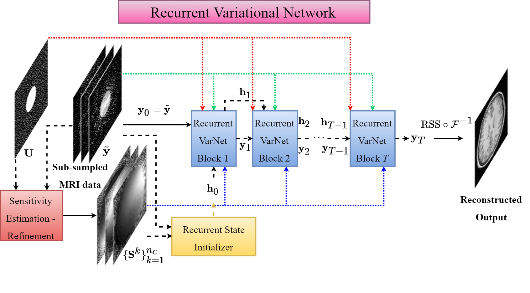
The RecurrentVarNet takes as input a multi-coil sub-sampled $k$-space $\tilde{\mathbf{y}}$ and outputs a reconstructed prediction of the ground truth image. It consists of the main block, Recurrent Variational Network Block (RecurrentVarNet Block), a Sensitivity Estimation and Refinement (SER) module, and a Recurrent State Initializer (RSI) module. The RecurrentVarNet Blocks produce intermediate $k$-space refinements of $\tilde{\mathbf{y}}$ following an unrolled iterative scheme of $T$ time-steps. The SER module estimates and refines (during training) the sensitivity map of each coil and the RSI module produces an initialization of the hidden or internal state of the first RecurrentVarNet Block. The above will be further defined in Sections 3.2, 3.4 and 3.3, respectively.

Note that our model uses as an initial guess of the $k$-space the sub-sampled $k$-space measurements $\mathbf{y}_{0}\,=\,\tilde{\mathbf{y}}$. In Fig. 2 we provide a comprehensive illustration of the architecture of our RecurrentVarNet.

3.2 Recurrent Variational Network Block

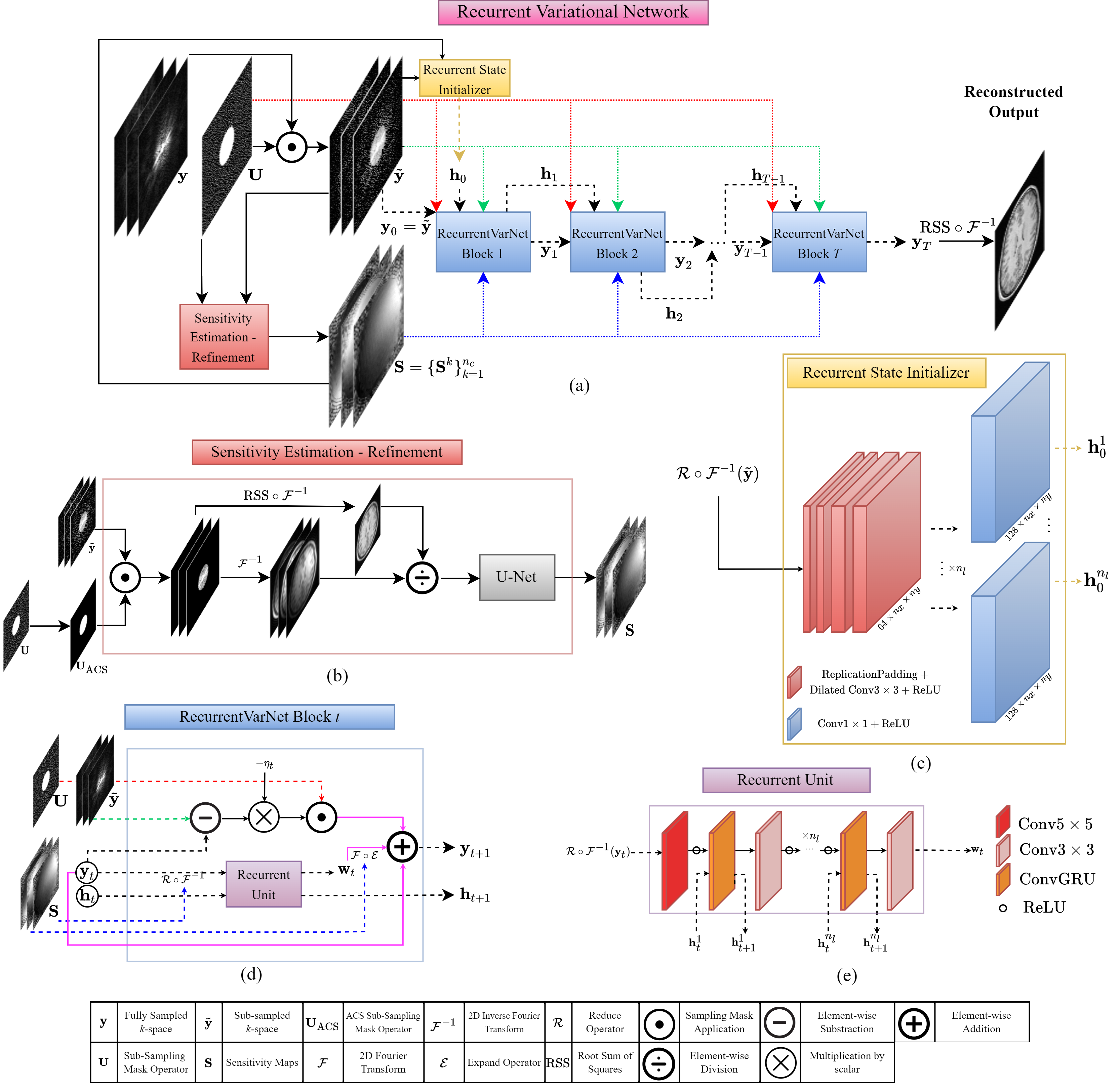
In this Section we formally introduce the main block of our proposed method: the Recurrent Variational Network Block. Following (14) we replaced $\mathcal{G}_{\theta_{t}}$ with a Recurrent Unit $\mathcal{H}_{\theta_{t}}$. The iterative optimization scheme of the RecurrentVarNet performed by the RecurrentVarNet Block (Fig. 2(d)) has the following form

$$\begin{gathered}\mathbf{w}_{t},\,\mathbf{h}_{t+1}\,=\,\mathcal{H}_{\theta_{t+1}}\Big{(}\mathcal{R}\,\circ\,\mathcal{F}^{-1}\big{(}\mathbf{y}_{t}\big{)},\,\mathbf{h}_{t}\Big{)}\\ \ vec{y}_{t+1}\,=\,\mathbf{y}_{t}\,-\,\alpha_{t+1}\,\mathbf{U}\big{(}\mathbf{y}_{t}\,-\,\tilde{\mathbf{y}}\big{)}\,+\,\mathcal{F}\,\circ\,\mathcal{E}\big{(}\mathbf{w}_{t}\big{)}.\\ \end{gathered}$$ (15)

Equation 15 comprises a data consistency term and a $k$-space refinement term. The latter projects the intermediate $k$-space prediction onto the image domain which in turn is fed to $\mathcal{H}_{\theta_{t}}$, whose output is projected back to the measurements domain, making RecurrentVarNet a hybrid domain-learning model.

Contrary to other CNN-based architectures and similarly to recurrent neural networks, at each time-step $t$ of the unrolled optimization scheme our recurrent unit $\mathcal{H}_{\theta_{t}}$ takes additionally as input a hidden state $\mathbf{h}_{t-1}$ that stores the sequence information up to time-step $t-1$ and outputs the next $\mathbf{h}_{t}\,=\,(\mathbf{h}_{t}^{1},\,...,\,\mathbf{h}_{t}^{n_{l}})$. The initial hidden state $\mathbf{h}_{0}$ is produced by the learned RSI unit (introduced in Sec. 3.3).

As depicted in Fig. 2(e), the recurrent unit $\mathcal{H}_{\theta_{t}}$ of RecurrentVarNet Block consists of a two-dimensional $5\times 5$ convolution (Conv$5\times 5$), followed by a sequence of $n_{l}$ alternating layers of two-dimensional $3\times 3$ convolutions (Conv$3\times 3$) and ConvGRUs [34]. A ReLU activation function is applied after each convolution except the last. At each time-step $t$, each ConvGRU at a layer $i\,=\,1,\,...,\,n_{l}$ uses $h_{t-1}^{i}$ as an internal state produced from the corresponding layer $i$ of the previous time-step and outputs $h_{t}^{i}$ for the next time-step. In addition, for each block a trainable parameter posing as the step size $\alpha_{t}\,=\,\alpha_{\theta_{t}}$ at each iteration is learned which is initialized as 1.0.

3.3 Recurrent State Initializer

Each RecurrentVarNet Block is fed with the previous internal state and outputs the next. In our framework we employed a Recurrent State Initializer (RSI) that learns to initialize the hidden state $\mathbf{h}_{0}$ inputted in the first RecurrentVarNet Block based on the sub-sampled input $\mathbf{y}_{0}\,=\,\tilde{\mathbf{y}}$. As an input to the RSI module we used a SENSE reconstruction

$$\mathcal{R}\circ\mathcal{F}^{-1}(\mathbf{y}_{0})\,=\,\sum_{k=1}^{n_{c}}{\mathbf{S}^{k}}^{*}\mathcal{F}^{-1}(\mathbf{y}_{0}^{k}).$$ (16)

As an alternative to (16), a zero-filled root-sum-of-squares reconstruction can be used

$$\text{RSS}\circ\mathcal{F}^{-1}(\mathbf{y}_{0})\,=\ \text{RSS}\big{(}\mathcal{F}^{-1}(\mathbf{y}_{0}^{1}),\,...,\,\mathcal{F}^{-1}(\mathbf{y}_{0}^{n_{c}})\big{)},$$ (17)

but our experiments have shown superior performance when using the SENSE input.

Our Recurrent State Initializer was inspired by the works in [35] and it incorporates a sequence of four layers of a replication padding (ReplicationPadding) module [36] of size $p$ followed by a two-dimensional $3\times 3$ dilated convolution with $p$ dilations and $n_{d}$ filters. Subsequently, the output is fed into $n_{l}$ two-dimensional $1\times 1$ convolutions followed by a ReLU activation to produce the initial hidden state $\mathbf{h}_{0}\,=\,(\mathbf{h}_{0}^{1},\,...,\,\mathbf{h}_{0}^{n_{l}})$. Figure 2(c) provides an illustration of RSI’s architecture.

3.4 Sensitivity Estimation - Refinement

For highly sub-sampled data using only the auto-calibration method as described by (5) fails to produce accurate estimations of the coil sensitivity maps. For that reason, to estimate and refine the sensitivity map of each coil the RecurrentVarNet employs a Sensitivity Estimation - Refinement (SER) module which is jointly trained with the rest of the blocks of the model. Specifically, SER takes as input the sub-sampled $k$-space $\tilde{\mathbf{y}}$ and estimates an initial approximation of the sensitivity maps as in (5). Afterwards, this initial approximation is fed into a U-Net (denoted as $\mathcal{S}_{\theta_{s}}$) which refines the sensitivity maps even further:

$$\mathbf{S}^{k}\,=\,\mathcal{S}_{\theta_{s}}(\tilde{\mathbf{S}}^{k}).$$ (18)

An overview of the SER module is depicted by Fig. 2(b). Our U-Net implementation uses leaky-ReLU as activation instead of ReLU and performs instance normalization after each convolution.

3.5 Training Loss Function

As aforementioned, our proposed model is fed with the sub-sampled $k$-space $\tilde{\mathbf{y}}$ as input and outputs at the last iteration a prediction $\mathbf{y}_{T}$ of the fully sampled $k$-space. For the reference or ground truth image we utilized the RSS reconstruction using the fully sampled measurements $\mathbf{y}$ calculated as $\bar{\mathbf{x}}\,=\,\text{RSS}\circ\mathcal{F}^{-1}(\mathbf{y})$.

Our model is trained end-to-end. As a training loss function we employed a custom-made function $\tilde{\mathcal{L}}$ as the sum of the $\mathcal{L}_{1}$ loss and a loss derived from the Structural Similarity Index Measure (SSIM) metric [37], denoted as $\mathcal{L}_{\text{SSIM}}$. The loss was calculated as follows:

$$\begin{gathered}\tilde{\mathcal{L}}(\bar{\mathbf{x}},\,\mathbf{x}_{T})\,=\,w_{1}\mathcal{L}_{1}(\bar{\mathbf{x}},\,\mathbf{x}_{T})\,+w_{2}\,\mathcal{L}_{\text{SSIM}}(\bar{\mathbf{x}},\,\mathbf{x}_{T})\\ =\,w_{1}||\bar{\mathbf{x}}\,-\,\mathbf{x}_{T}||_{1}\,+\,w_{2}(1-\text{SSIM}(\bar{\mathbf{x}},\,\mathbf{x}_{T}))\end{gathered}$$ (19)

where

$$\mathbf{x}_{T}\,=\,\text{RSS}\circ\mathcal{F}^{-1}(\mathbf{y}_{T}),$$ (20)

and $0\leq w_{1},\,w_{2}\leq 1$ are multiplying factors.

4 Experiments

4.1 Implementation

4.1.1 RecurrentVarNet Implementation

To avoid problems occurring from holomorphic differentiation of complex-valued data, we converted all complex-valued data to real-valued by concatenating the real and imaginary parts into the channels (= 2) dimensions. For instance, the masked $k$-space had the following form:

$$\tilde{\vec{y}}\,=\,\big{(}\text{Re}(\tilde{\vec{y}}),\,\text{Im}(\tilde{\vec{y}})\big{)}\,\in\,\mathbb{R}^{2\times n\times n_{c}}.$$

Similarly, all operators and models operated in the real-valued domain. For instance,

$$\mathcal{A}:\mathbb{R}^{2\times n}\rightarrow\mathbb{R}^{2\times n\times n_{c}},\quad\mathcal{A}^{*}:\mathbb{R}^{2\times n\times n_{c}}\rightarrow\mathbb{R}^{2\times n}.$$

With the above modification, our model works with multi-coil $k$-space data of arbitrary number of coils. Therefore, there is no need for prerequisite knowledge of the type of the MRI scanner.

Our model was implemented using PyTorch [38]. Our code and models including all state of the art baselines are available under the Apache 2.0 licence in our Deep Image Reconstruction Toolkit (DIRECT) [39]. For our experiments we used $T\,=\,8$ optimization steps (and RecurrentVarNet Blocks) and chose 128 channels for the size of the hidden state. Also, we set $n_{l}\,=\,4$ for the recurrent unit of RecurrentVarNet Block. For the RSI module as the values of $p$ and $n_{d}$ in each of the four layers we used (1, 1, 2, 4) dilations and (32, 32, 64, 64) filters, respectively, and used convolutions with 128 filters in the output layer. For $\mathcal{S}_{\theta_{s}}$ in the SER module we employed a U-Net with four scales with 8, 16, 32 and 64 number of filters for the convolutions, zero dropout probability, and 0.2 negative slope coefficient for the leaky-ReLU activation.

4.1.2 Dataset

Figure 3: Reconstructed slices with the RSS method of fully-sampled brain slices from the Calgary-Campinas brain dataset.

For our experiments we utilized the public Calgary-Campinas dataset [40] which was released as part of the Multi-Coil MRI (MC-MRI) Reconstruction Challenge [18]. The dataset contains three-dimensional volumes of raw fully-sampled $k$-space measurements which are T1-weighted, gradient-recalled echo, 1 mm isotropic sagittal, acquired on 1.5T or 3T MRI scanners.

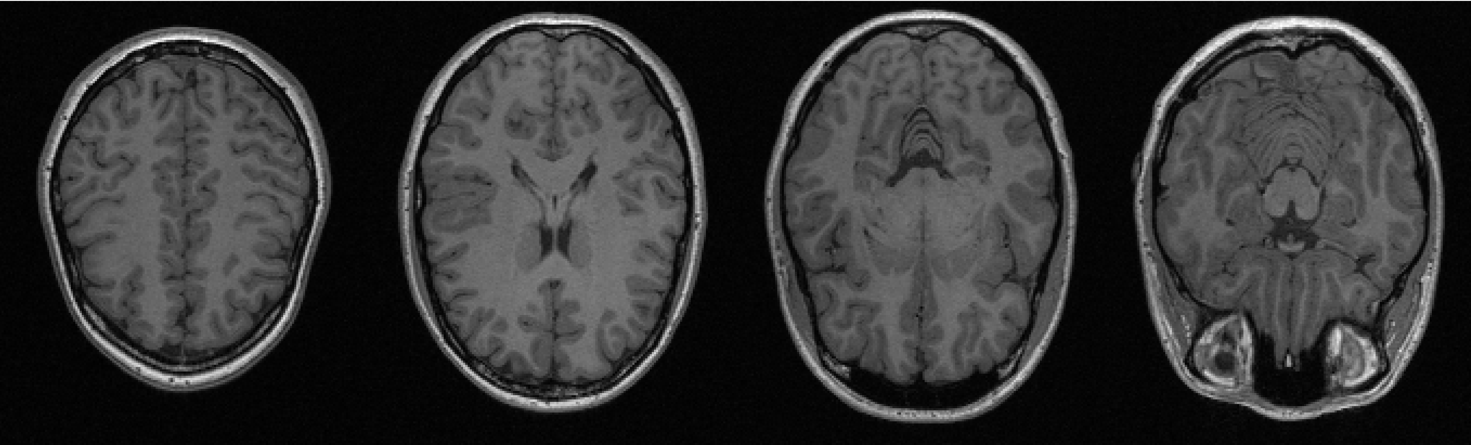
We employed only the provided training (47 volumes, 7332 axial slices) and validation (20 volumes, 3120 axial slices) sets of the dataset (fully-sampled test set is not yet publicly available) which amounted to 67 volumes of $n_{c}=12$ multi-coil data. We split the validation set in half to create a new validation set (10 volumes of 1560 axial slices) and a test set (10 volumes of 1560 axial slices). Reconstructed images have $218\times$ $170$/$180$ pixels. Some instances of reconstructed slices are illustrated in Fig. 3.

4.1.3 Sub-sampling

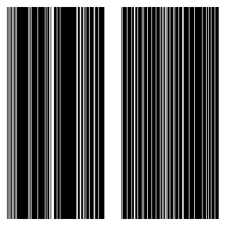
We retrospectively sub-sampled the fully-sampled data setting as acceleration factors $R=5$ and $R=10$ and using sub-sampling masks provided by the Calgary-Campinas MC-MRI Reconstruction Challenge.

Figure 4: Sub-sampling mask

Figure 4 depicts an example of a sub-sampling mask used. During training, data were arbitrarily 5-fold or 10-fold sub-sampled, and for evaluation and testing, data were both 5 and 10-fold sub-sampled.

4.1.4 Training Details

Our model was optimized using the Adam optimizer with parameters $\beta_{1}\,=\,0.9$, $\beta_{2}\,=\,0.999$ and $\epsilon\,=\,1\text{e}-8$ with a batch size of 4 two-dimensional slices for 63000 iterations which amounted to approximately 270 epochs. A warm-up schedule [41] was used to linearly increase the learning rate to 0.0005 over 1000 warm-up iterations. The learning rate was decayed by a factor of 0.2 every 20000 training iterations. For the training we employed eight NVIDIA RTX A6000 GPUs.

For the training loss function we set both multiplying factors to $w_{1},\,w_{2}\,=\,1.0$. The total number of trainable parameters for our model with the choice of hyper-parameters as described in Sec. 4.1.1 amounted to approximately 7400k parameters.

Figure 5: Reconstructed slices from the test set along with zoomed-in regions of interest using an acceleration factor of $R\,=\,5$. (a) Ground Truth, (b) Zero-filled reconstruction, (c) U-Net, (d) End-to-End Variational Network, (e) XPDNet, (f) Recurrent Inference Machine, (g) Ours: Recurrent Variational Network.

4.1.5 Evaluation Metrics

To evaluate the quality of the reconstructions we employed three commonly used in image reconstruction assessment metrics: the SSIM metric, the peak signal-to-noise ratio (pSNR) [42], and the normalized mean squared error (NMSE) [43]. The metrics were computed using the reference RSS reconstructions of the fully-sampled data and the predicted RSS reconstructions.

4.2 Experimental Results

Acceleration Factor	Model	Metrics
		SSIM $\uparrow$	pSNR $\uparrow$	NMSE $\downarrow$
$R\,=\,5$	Zero-Filled	0.7371	25.27	0.0401
	U-Net	0.8682	29.25	0.0210
	E2EVarNet	0.9073	32.62	0.0086
	XPDNet	0.9325	34.80	0.0051
	RIM	0.9381	35.61	0.0042
	RecurrentVarNet	0.9418	36.02	0.0038
$R\,=\,10$	Zero-Filled	0.6905	24.35	0.0527
	U-Net	0.8177	27.23	0.0308
	E2EVarNet	0.8610	29.85	0.0158
	XPDNet	0.8949	31.76	0.0105
	RIM	0.9047	32.52	0.0089
	RecurrentVarNet	0.9073	32.71	0.0085

Table 1: Quantitative evaluation using three evaluation metrics for two acceleration factors $R\,=\,5,\,10$.

4.2.1 Comparisons

To evaluate the performance of our proposed model we made comparisons against reconstructions output from the following models:

• A U-Net with four scales consisted of 64, 128, 256, and 512 convolution filters respectively.

• An End-to-End Variational Network with the same choice of hyper-parameters as in the published work [21].

• An XPDNet [20] with 10 iterations, 5 primal and 5 dual layers and U-Nets for the primal and dual models.

• A Recurrent Inference Machine with 16 time-steps and 128 features [22].

All models were trained on the training set by arbitrarily setting $R$ to 5 or 10, and were optimized in similar fashion to Sec. 4.1.4. Additionally, all models were trained jointly with a U-Net that estimated and refined the sensitivity maps with the same choice of hyper-parameters as our SER module. We also compared RecurrentVarNet’s reconstructions against Zero-Filled reconstructions (we used $\text{RSS}\circ\mathcal{F}^{-1}(\tilde{\mathbf{y}})$). In the following paragraphs we provide quantitative and qualitative results and comparisons.

Quantitative Results

In Tab. 1 are presented the quantitative results of our experiments for both acceleration factors and are reported the average evaluation metrics obtained on the test set. To obtain these results we used the best-performing checkpointed model according to the validation results on the SSIM metric. Compared against the other methods, RecurrentVarNet marked the highest average SSIM and pSNR metrics, as well as the lowest average NMSE metric, highlighting its superior performance.

Qualitative Results

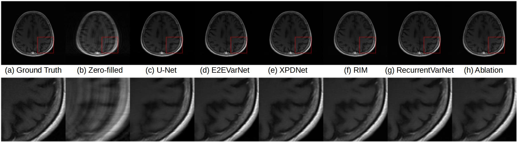
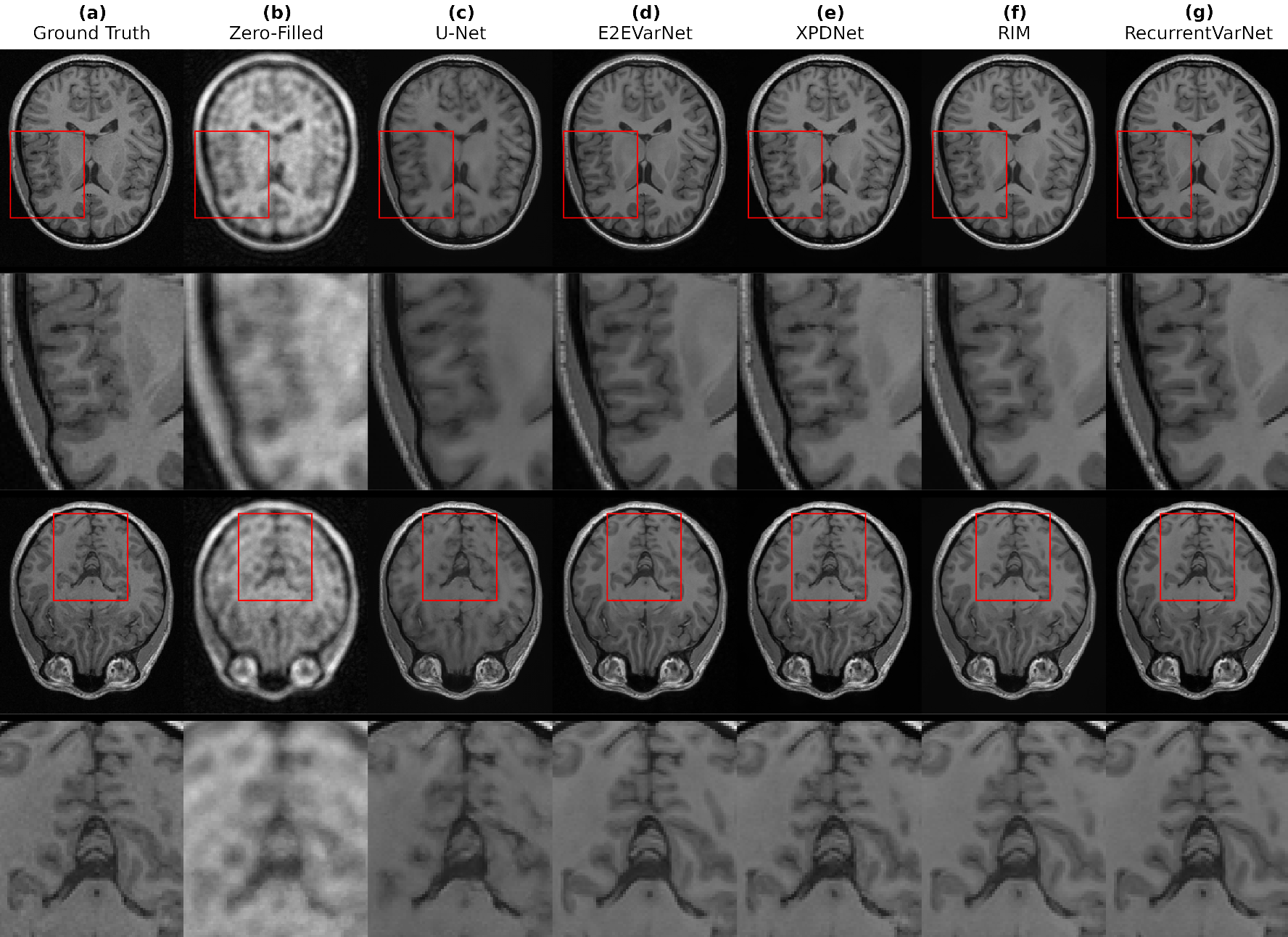
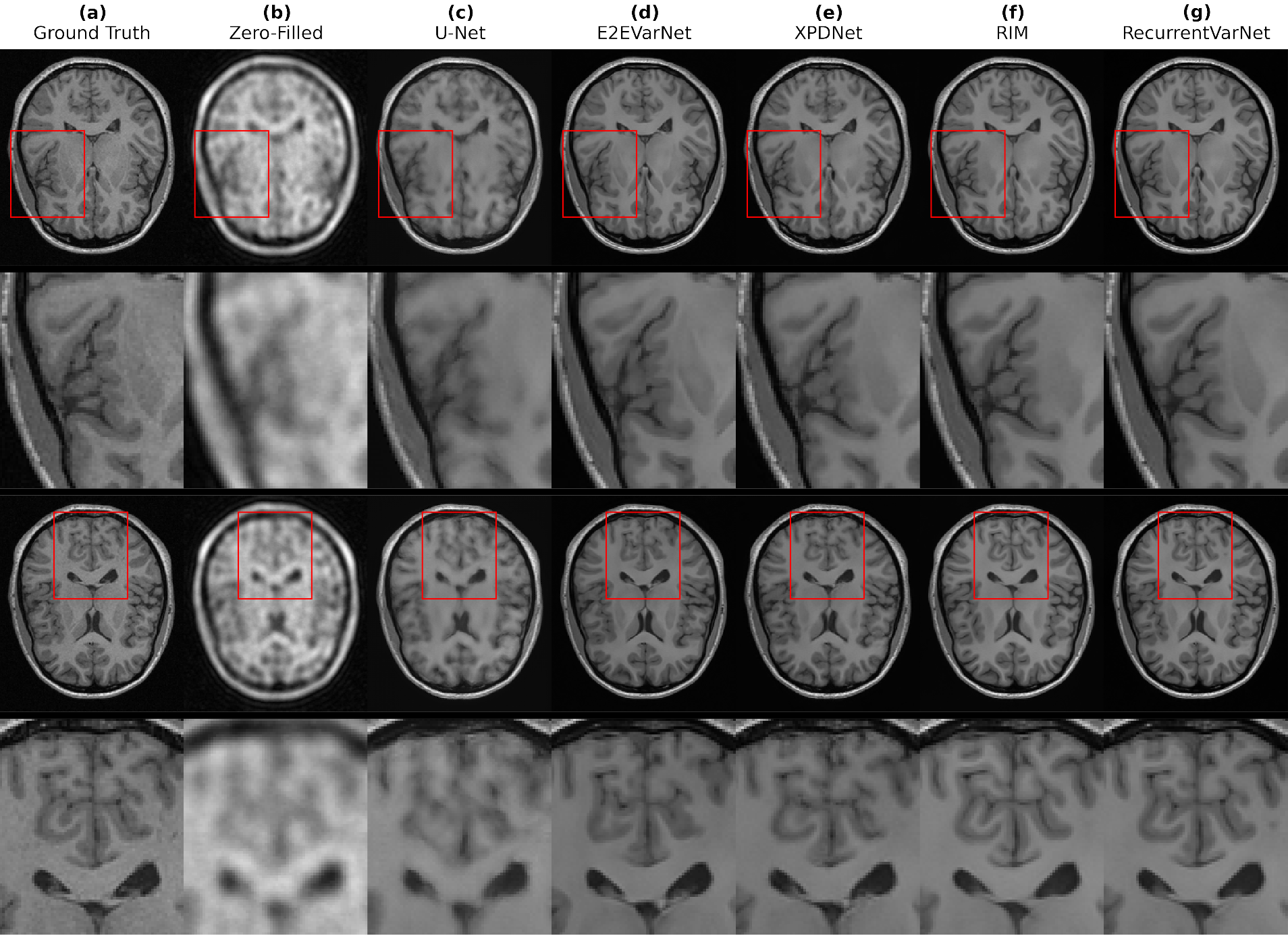
To asses the quality of the RecurrentVarNet’s reconstructions we visualized in Fig. 5 two reconstructed samples with the RSS method from the test set which were 5-fold sub-sampled. For comparisons, we also visualized the ground truth images, the images reconstructed from the sub-sampled data (Zero-Filled), and the trained models U-Net, E2EVarNet, XPDNet, and RIM. In contrast with the rest of the reconstructions, our method produced images that matched the ground truth images better as shown by the zoomed-in regions of interest in Fig. 5. Visualizations for $R\,=\,10$ can be found in the Supplementary Material.

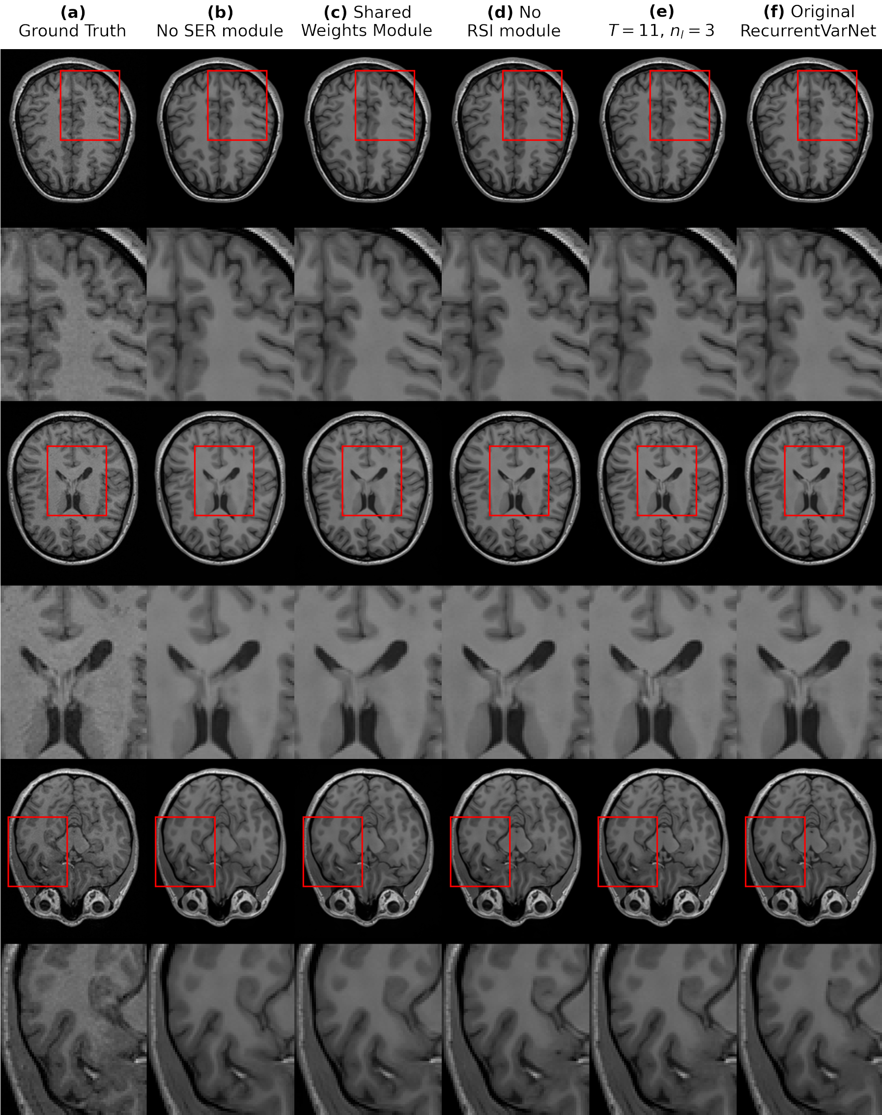
4.2.2 Ablation Study

Acceleration Factor	RecurrentVarNet	Metrics
		SSIM $\uparrow$	pSNR $\uparrow$	NMSE $\downarrow$
$R\,=\,5$	No SER module	0.9374	35.52	0.0043
	Shared weights	0.9386	35.66	0.0041
	No RSI module	0.9411	35.93	0.0039
	$T\,=\,11,\quad n_{l}\,=\,3$	0.9417	35.99	0.0037
	Original	0.9418	36.02	0.0038
$R\,=\,10$	No SER module	0.8960	32.04	0.0099
	Shared weights	0.9017	32.37	0.0092
	No RSI module	0.9071	32.69	0.0085
	$T\,=\,11,\quad n_{l}\,=\,3$	0.9093	32.83	0.0082
	Original	0.9073	32.71	0.0084

Table 2: Ablation Study of RecurrentVarNet: Quantitative results of $5$-fold and $10$-fold accelerated reconstructions using four distinct implementations of the RecurrentVarNet.

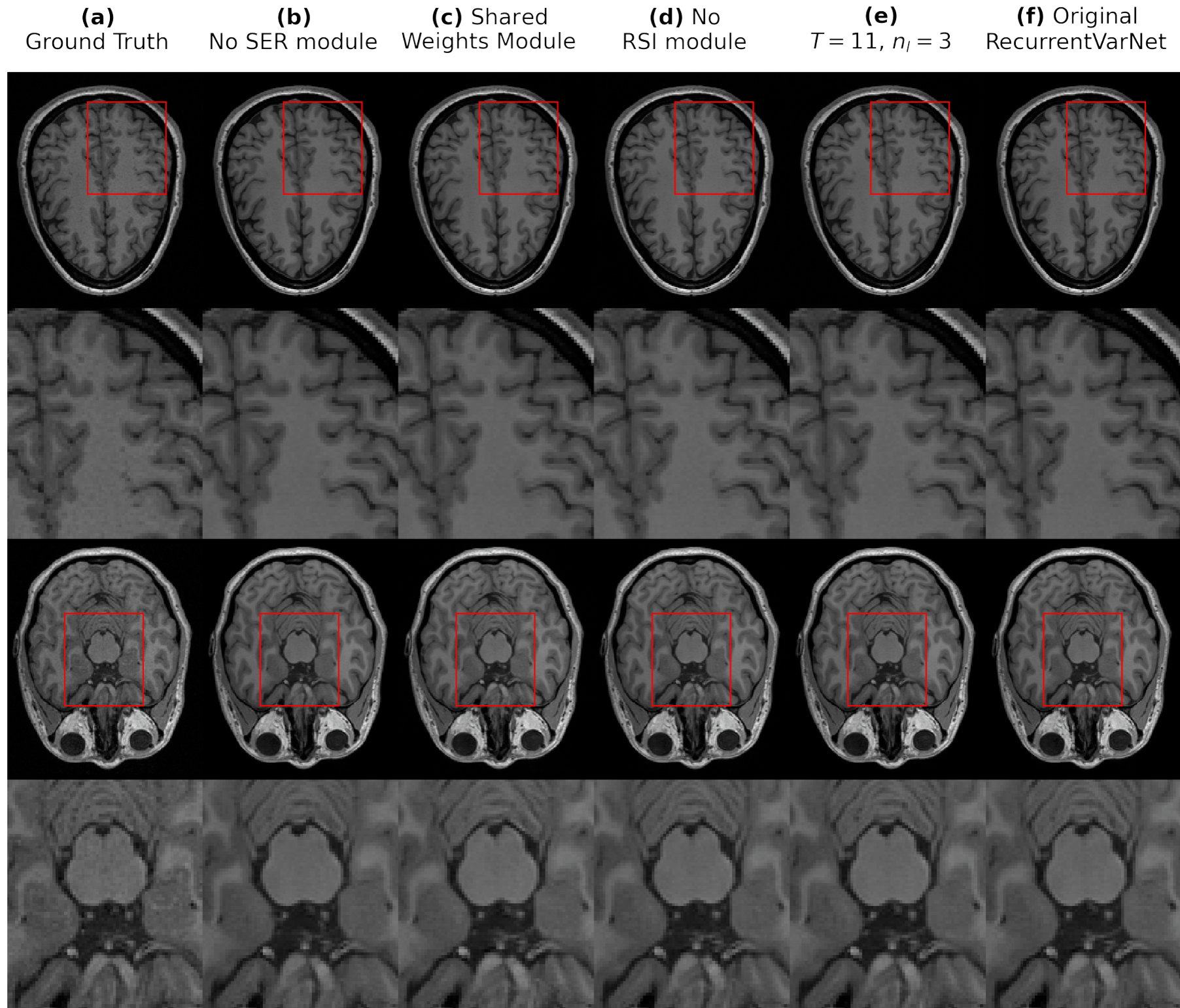
To investigate the performance of our RecurrentVarNet even further, we compared the original implementation with different choices of hyper-parameters. More specifically, we compared it against four distinct cases:

• A RecurrentVarNet without a SER module. In this case, the sensitivity maps were estimated as in (5) with no refinement performed.

• A RecurrentVarNet without a RSI module. The hidden state was initialized as a vector of zeros.

• A RecurrentVarNet with the same number of RecurrentVarNet Blocks, but with shared weights for the Recurrent Unit that is, $\mathcal{H}_{\theta_{t}}\,=\,\mathcal{H}_{\theta}$ for all $t\,=\,1,\,...,\,T$.

• A RecurrentVarNet with higher number of RecurrentVarNet Blocks ($T\,=\,11$) and less layers in the Recurrent Unit ($n_{l}\,=\,3$).

For the ablation study due to space limitation we chose to present here only the quantitative comparisons of the original implementation with the four modifications, and we include the qualitative comparisons in the Supplementary Material. Similarly to Sec. 4.2.1, we utilized the best model checkpoints to acquire the evaluation metrics. In Tab. 2 we report the average SSIM, pSNR and NMSE metrics acquired from the reconstructions of the 5-fold and 10-fold accelerated test set.

In general, our original model exhibited superior performance for both acceleration factors, therefore, our original implementation is well-justified. It should be noted that the RecurrentVarNet with the choice of $T\,=\,11$ and $n_{l}\,=\,3$ performed slightly better in the case of $R\,=\,10$, which can be attributed to the fact that more optimization steps were used. However, our original architecture was the model of choice since the model with $T\,=\,11$ and $n_{l}\,=\,3$ required more memory during training due to its need to accumulate more gradients in memory to perform the back-propagation when computing the loss function.

5 Conclusions

In this work, we have proposed a novel deep learning image inverse problem solver architecture, the Recurrent Variational Network, which we particularized to the task of reconstructing MR images from accelerated multi-coil $k$-space measurements. The quantitative and qualitative results of our experiments have demonstrated that the RecurrentVarNet outperformed state of the art approaches, which can be attributed to its hybrid nature, since its main block performs iterative optimization in the $k$-space domain using a recurrent unit operating in the image domain.

Recurrent Variational Network: A Deep Learning Inverse Problem Solver applied to the task of Accelerated MRI Reconstruction
Supplementary Material

Appendix A Additional Figures

A.1 Comparisons - Qualitative Results

Figure 6: Reconstructed slices from the test set along with zoomed-in regions of interest using an acceleration factor of $R\,=\,10$. (a) Ground Truth, (b) Zero-filled reconstruction, (c) U-Net, (d) End-to-End Variational Network, (e) XPDNet, (f) Recurrent Inference Machine, (g) Ours: Recurrent Variational Network.

A.2 Ablation Study - Qualitative Results

Figure 7: Reconstructed slices from the test set along with zoomed-in regions of interest using an acceleration factor of $R\,=\,5$. (a) Ground Truth, (b) ReccurentVarNet without a Sensitivity Estimation - Refinement module, (c) ReccurentVarNet with shared weights for the Recurrent Units, (d) ReccurentVarNet without a Recurrent State Initializer, (e) ReccurentVarNet with $T\,=\,11$ and $n_{l}\,=\,3$, (f) Original Recurrent Variational Network.

Figure 8: Reconstructed slices from the test set along with zoomed-in regions of interest using an acceleration factor of $R\,=\,10$. (a) Ground Truth, (b) ReccurentVarNet without a Sensitivity Estimation - Refinement module, (c) ReccurentVarNet with shared weights for the Recurrent Units, (d) ReccurentVarNet without a Recurrent State Initializer, (e) ReccurentVarNet with $T\,=\,11$ and $n_{l}\,=\,3$, (f) Original Recurrent Variational Network.

Appendix B Additional Experiments

In this Section we provide additional experiments for our proposed method using the fastMRI AXT1 multi-coil brain dataset [1].

B.1 Dataset description

The fastMRI AXT1 multi-coil brain dataset is consisted of 248 training volumes (3844 slices) and 82 validation (1424 slices) validation volumes which we split in half to create new validation and test sets (41 volumes/712 slices each).

B.2 Sub-sampling

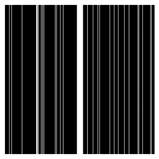
The data were retrospectively sub-sampled for $R=4$ and $R=8$ using random Cartesian masks provided by the fastMRI challenge. The sub-sampling masks were produced by first sampling a fraction of the low frequencies or the ACS region (8% when $R=4$ and 4% when $R=8$) and then randomly sampling up to the level of acceleration $R$. An example of each mask is depicted in Fig. 9.

(a) $R=4$ with 8% of ACS region.

(b) $R=8$ with 4% of ACS region.

Figure 9: Random Cartesian sub-sampling masks.

B.3 Comparison & Ablation Study

We employed a RecurrentVarNet with $T=8$ time-steps, 92 filters for the hidden state $\mathbf{h}_{t}$, and $n_{l}=3$. For comparisons we used:

• A U-Net with 32, 64, 128, 256 convolution filters in each scale.

• An E2EVarNet with 6 layers and 16, 32, 64, 128 filters for the scales of the U-Net regularizer.

• An XPDNet with 6 iterations and 5 primal and 5 dual layers with U-Nets for the primal and dual models.

• A RIM with 8 time-steps and 64 features.

For the ablation study we employed a RecurrentVarNet with $T=6$ time-steps, 128 filters for $\mathbf{h}_{t}$, and $n_{l}=2$.

All models were trained on four NVIDIA RTX A6000 GPUs. The RecurrentVarNet with $T=8$ and the XPDNet were trained for 120k iterations, while the rest of the aforementioned models were trained for 180k iterations.

Note that for our experiments on the fastMRI dataset we used a lower number of parameters than for those on the Calgary Campinas dataset due to the fact that the fastMRI slices have approximately $6\times$ more pixels and, hence, require approximately $6\times$ more GPU memory.

Quantitative results

Model	Metrics
	$R=4$			$R=8$
	SSIM $\uparrow$	pSNR $\uparrow$	NMSE $\downarrow$	SSIM $\uparrow$	pSNR $\uparrow$	NMSE $\downarrow$
Zero-Filled	0.813	30.77	0.039	0.708	26.21	0.096
U-Net	0.943	37.09	0.012	0.922	34.41	0.021
E2EVarNet	0.959	40.83	0.005	0.940	37.35	0.011
XPDNet	0.958	40.93	0.005	0.941	37.83	0.010
RIM	0.957	40.84	0.005	0.938	37.36	0.011
RecurrentVarNet	0.960	41.28	0.005	0.941	37.69	0.010
RecurrentVarNet (ablation)	0.959	40.95	0.005	0.938	37.31	0.011

Table 3: Quantitative evaluation using three evaluation metrics for two acceleration factors $R\,=\,4,\,8$ on the fastMRI AXT1 test set.

In Tab. 3 are reported the average evaluation metrics obtained on the test set for both acceleration factors.

Qualitative results

In Fig. 10 are visualized reconstructed slices with the RSS method from one sample from the test set for $R=4$.

Figure 10: Reconstructed slice from the fastMRI AXT1 test set along with zoomed-in regions of interest using an acceleration factor of $R\,=\,4$. (a) Ground Truth, (b) Zero-filled reconstruction, (c) U-Net, (d) End-to-End Variational Network, (e) XPDNet, (f) Recurrent Inference Machine, (g) Ours: Recurrent Variational Network, (h) Recurrent Variational Network (ablation).

References

- [1] Jure Zbontar, Florian Knoll, Anuroop Sriram, Tullie Murrell, Zhengnan Huang, Matthew J. Muckley, Aaron Defazio, Ruben Stern, Patricia Johnson, Mary Bruno, Marc Parente, Krzysztof J. Geras, Joe Katsnelson, Hersh Chandarana, Zizhao Zhang, Michal Drozdzal, Adriana Romero, Michael Rabbat, Pascal Vincent, Nafissa Yakubova, James Pinkerton, Duo Wang, Erich Owens, C. Lawrence Zitnick, Michael P. Recht, Daniel K. Sodickson, and Yvonne W. Lui. fastmri: An open dataset and benchmarks for accelerated mri, 2019.
- [2] David J. Larkman and Rita Gouveia Nunes. Parallel magnetic resonance imaging. Physics in medicine and biology, 52 7:R15–55, 2007.
- [3] Klaas Pruessmann. Encoding and reconstruction in parallel mri. NMR in biomedicine, 19:288–99, 05 2006.
- [4] Michael Lustig and John Pauly. Spirit: Iterative self-consistent parallel imaging reconstruction from arbitrary k-space. Magnetic resonance in medicine : official journal of the Society of Magnetic Resonance in Medicine / Society of Magnetic Resonance in Medicine, 64:457–71, 08 2010.
- [5] Michael Lustig, David Donoho, and John M. Pauly. Sparse mri: The application of compressed sensing for rapid mr imaging. Magnetic Resonance in Medicine, 58(6):1182–1195, 2007.
- [6] D.L. Donoho. Compressed sensing. IEEE Transactions on Information Theory, 52(4):1289–1306, 2006.
- [7] Ricardo Otazo, Li Feng, Hersh Chandarana, Tobias Block, Leon Axel, and Daniel K. Sodickson. Combination of compressed sensing and parallel imaging for highly-accelerated dynamic mri. In 2012 9th IEEE International Symposium on Biomedical Imaging (ISBI), pages 980–983, 2012.
- [8] Martin Uecker, Peng Lai, M. J. Murphy, Patrick Virtue, Michael Elad, John M. Pauly, Shreyas S. Vasanawala, and Michael Lustig. Espirit—an eigenvalue approach to autocalibrating parallel mri: Where sense meets grappa. Magnetic Resonance in Medicine, 71, 2014.
- [9] Angshul Majumdar and Rabab K. Ward. Iterative estimation of mri sensitivity maps and image based on sense reconstruction method (isense). Concepts in Magnetic Resonance Part A, 40A(6):269–280, 2012.
- [10] Klaas P. Pruessmann, Markus Weiger, Markus B. Scheidegger, and Peter Boesiger. Sense: Sensitivity encoding for fast mri. Magnetic Resonance in Medicine, 42(5):952–962, 1999.
- [11] Mark Griswold, Peter Jakob, Robin Heidemann, Mathias Nittka, Vladimir Jellus, Jianmin Wang, Berthold Kiefer, and Axel Haase. Generalized autocalibrating partially parallel acquisitions (grappa). Magnetic resonance in medicine : official journal of the Society of Magnetic Resonance in Medicine / Society of Magnetic Resonance in Medicine, 47:1202–10, 06 2002.
- [12] Daniel K. Sodickson and Warren J. Manning. Simultaneous acquisition of spatial harmonics (smash): Fast imaging with radiofrequency coil arrays. Magnetic Resonance in Medicine, 38(4):591–603, 1997.
- [13] John N. Morelli, Val M. Runge, Fei Ai, Ulrike Attenberger, Lan Vu, Stuart H. Schmeets, Wolfgang R. Nitz, and John E. Kirsch. An image-based approach to understanding the physics of mr artifacts. RadioGraphics, 31(3):849–866, 2011. PMID: 21571661.
- [14] U. Grenander, H. Cramér, and Karreman Mathematics Research Collection. Probability and Statistics: The Harald Cramér Volume. Wiley publications in statistics. Almqvist & Wiksell, 1959.
- [15] C.E. Shannon. Communication in the presence of noise. Proceedings of the IRE, 37(1):10–21, 1949.
- [16] Aurélien Bustin, Niccolo Fuin, Rene Botnar, and Claudia Prieto. From compressed-sensing to artificial intelligence-based cardiac mri reconstruction. Frontiers in Cardiovascular Medicine, 7:17, 02 2020.
- [17] Matthew J. Muckley, Bruno Riemenschneider, Alireza Radmanesh, Sunwoo Kim, Geunu Jeong, Jingyu Ko, Yohan Jun, Hyungseob Shin, Dosik Hwang, Mahmoud Mostapha, and et al. Results of the 2020 fastmri challenge for machine learning mr image reconstruction. IEEE Transactions on Medical Imaging, 40(9):2306–2317, Sep 2021.
- [18] Youssef Beauferris, Jonas Teuwen, Dimitrios Karkalousos, Nikita Moriakov, Matthan Caan, George Yiasemis, Lívia Rodrigues, Alexandre Lopes, Hélio Pedrini, Letícia Rittner, Maik Dannecker, Viktor Studenyak, Fabian Gröger, Devendra Vyas, Shahrooz Faghih-Roohi, Amrit Kumar Jethi, Jaya Chandra Raju, Mohanasankar Sivaprakasam, Mike Lasby, Nikita Nogovitsyn, Wallace Loos, Richard Frayne, and Roberto Souza. Multi-coil mri reconstruction challenge – assessing brain mri reconstruction models and their generalizability to varying coil configurations, 2021.
- [19] Taejoon Eo, Yohan Jun, Taeseong Kim, Jinseong Jang, Ho-Joon Lee, and Dosik Hwang. Kiki-net: cross-domain convolutional neural networks for reconstructing undersampled magnetic resonance images. Magnetic Resonance in Medicine, 80(5):2188–2201, 2018.
- [20] Zaccharie Ramzi, Philippe Ciuciu, and Jean-Luc Starck. Xpdnet for mri reconstruction: an application to the 2020 fastmri challenge, 2021.
- [21] Anuroop Sriram, Jure Zbontar, Tullie Murrell, Aaron Defazio, C. Lawrence Zitnick, Nafissa Yakubova, Florian Knoll, and Patricia Johnson. End-to-end variational networks for accelerated mri reconstruction, 2020.
- [22] Kai Lønning, Patrick Putzky, Jan-Jakob Sonke, Liesbeth Reneman, Matthan W.A. Caan, and Max Welling. Recurrent inference machines for reconstructing heterogeneous mri data. Medical Image Analysis, 53:64–78, 2019.
- [23] Yohan Jun, Hyungseob Shin, Taejoon Eo, and Dosik Hwang. Joint deep model-based mr image and coil sensitivity reconstruction network (joint-icnet) for fast mri. In Proceedings of the IEEE/CVF Conference on Computer Vision and Pattern Recognition (CVPR), pages 5270–5279, June 2021.
- [24] Kerstin Hammernik, Teresa Klatzer, Erich Kobler, Michael P Recht, Daniel K Sodickson, Thomas Pock, and Florian Knoll. Learning a variational network for reconstruction of accelerated mri data, 2017.
- [25] Patrick Putzky and Max Welling. Recurrent inference machines for solving inverse problems, 2017.
- [26] Erik G. Larsson, Deniz Erdogmus, Rui Yan, Jose C. Principe, and Jeffrey R. Fitzsimmons. Snr-optimality of sum-of-squares reconstruction for phased-array magnetic resonance imaging. Journal of Magnetic Resonance, 163(1):121–123, 2003.
- [27] Xiaofang Liu, Wenlong Xu, and Xiuzi Ye. The ill-posed problem and regularization in parallel magnetic resonance imaging. In 2009 3rd International Conference on Bioinformatics and Biomedical Engineering, pages 1–4, 2009.
- [28] Jari Kaipio and Erkki Somersalo. Statistical and Computational Inverse Problems. Springer, Dordrecht, 2005.
- [29] Pengyue Zhang, Fusheng Wang, Wei Xu, and Yu Li. Multi-channel generative adversarial network for parallel magnetic resonance image reconstruction in k-space. In Alejandro F. Frangi, Julia A. Schnabel, Christos Davatzikos, Carlos Alberola-López, and Gabor Fichtinger, editors, Medical Image Computing and Computer Assisted Intervention – MICCAI 2018, pages 180–188, Cham, 2018. Springer International Publishing.
- [30] Mehmet Akçakaya, Steen Moeller, Sebastian Weingärtner, and Kâmil Uğurbil. Scan-specific robust artificial-neural-networks for k-space interpolation (raki) reconstruction: Database-free deep learning for fast imaging. Magnetic Resonance in Medicine, 81(1):439–453, 2019.
- [31] Tae Hyung Kim, Pratyush Garg, and Justin P. Haldar. Loraki: Autocalibrated recurrent neural networks for autoregressive mri reconstruction in k-space, 2019.
- [32] Jonas Adler and Ozan Oktem. Learned primal-dual reconstruction. IEEE Transactions on Medical Imaging, 37(6):1322–1332, Jun 2018.
- [33] Roberto Souza, Mariana Bento, Nikita Nogovitsyn, Kevin J. Chung, R. Marc Lebel, and Richard Frayne. Dual-domain cascade of u-nets for multi-channel magnetic resonance image reconstruction, 2019.
- [34] Emre Cakir, Giambattista Parascandolo, Toni Heittola, Heikki Huttunen, and Tuomas Virtanen. Convolutional recurrent neural networks for polyphonic sound event detection. IEEE/ACM Transactions on Audio, Speech, and Language Processing, 25(6):1291–1303, Jun 2017.
- [35] Fisher Yu and Vladlen Koltun. Multi-scale context aggregation by dilated convolutions, 2016.
- [36] Guilin Liu, Kevin J. Shih, Ting-Chun Wang, Fitsum A. Reda, Karan Sapra, Zhiding Yu, Andrew Tao, and Bryan Catanzaro. Partial convolution based padding, 2018.
- [37] Zhou Wang, A.C. Bovik, H.R. Sheikh, and E.P. Simoncelli. Image quality assessment: from error visibility to structural similarity. IEEE Transactions on Image Processing, 13(4):600–612, 2004.
- [38] Adam Paszke, Sam Gross, Francisco Massa, Adam Lerer, James Bradbury, Gregory Chanan, Trevor Killeen, Zeming Lin, Natalia Gimelshein, Luca Antiga, Alban Desmaison, Andreas Kopf, Edward Yang, Zachary DeVito, Martin Raison, Alykhan Tejani, Sasank Chilamkurthy, Benoit Steiner, Lu Fang, Junjie Bai, and Soumith Chintala. Pytorch: An imperative style, high-performance deep learning library. In Advances in Neural Information Processing Systems 32, pages 8024–8035. Curran Associates, Inc., 2019.
- [39] George Yiasemis, Nikita Moriakov, Dimitrios Karkalousos, Matthan Caan, and Jonas Teuwen. Direct: Deep image reconstruction toolkit. https://github.com/directgroup/direct, 2021.
- [40] Roberto Souza, Oeslle Lucena, Julia Garrafa, David Gobbi, Marina Saluzzi, Simone Appenzeller, Leticia Rittner, Richard Frayne, and Roberto Lotufo. An open, multi-vendor, multi-field-strength brain mr dataset and analysis of publicly available skull stripping methods agreement. NeuroImage, 170, 08 2017.
- [41] Priya Goyal, Piotr Dollár, Ross Girshick, Pieter Noordhuis, Lukasz Wesolowski, Aapo Kyrola, Andrew Tulloch, Yangqing Jia, and Kaiming He. Accurate, large minibatch sgd: Training imagenet in 1 hour, 2018.
- [42] Alain Horé and Djemel Ziou. Image quality metrics: Psnr vs. ssim. In 2010 20th International Conference on Pattern Recognition, pages 2366–2369, 2010.
- [43] Attilio Poli and Mario Cirillo. On the use of the normalized mean square error in evaluating dispersion model performance. Atmospheric Environment. Part A. General Topics, 27:2427–2434, 10 1993.