Improving Transferability of Representations
via Augmentation-Aware Self-Supervision

Abstract

Recent unsupervised representation learning methods have shown to be effective in a range of vision tasks by learning representations invariant to data augmentations such as random cropping and color jittering. However, such invariance could be harmful to downstream tasks if they rely on the characteristics of the data augmentations, e.g., location- or color-sensitive. This is not an issue just for unsupervised learning; we found that this occurs even in supervised learning because it also learns to predict the same label for all augmented samples of an instance. To avoid such failures and obtain more generalizable representations, we suggest to optimize an auxiliary self-supervised loss, coined AugSelf, that learns the difference of augmentation parameters (e.g., cropping positions, color adjustment intensities) between two randomly augmented samples. Our intuition is that AugSelf encourages to preserve augmentation-aware information in learned representations, which could be beneficial for their transferability. Furthermore, AugSelf can easily be incorporated into recent state-of-the-art representation learning methods with a negligible additional training cost. Extensive experiments demonstrate that our simple idea consistently improves the transferability of representations learned by supervised and unsupervised methods in various transfer learning scenarios. The code is available at https://github.com/hankook/AugSelf.

1 Introduction

Unsupervised representation learning has recently shown a remarkable success in various domains, e.g., computer vision [1, 2, 3], natural language [4, 5], code [6], reinforcement learning [7, 8, 9], and graphs [10]. The representations pretrained with a large number of unlabeled data have achieved outstanding performance in various downstream tasks, by either training task-specific layers on top of the model while freezing it or fine-tuning the entire model.

In the vision domain, the recent state-of-the-art methods [1, 2, 11, 12, 13] learn representations to be invariant to a pre-defined set of augmentations. The choice of the augmentations plays a crucial role in representation learning [2, 14, 15, 16]. A common choice is a combination of random cropping, horizontal flipping, color jittering, grayscaling, and Gaussian blurring. With this choice, learned representations are invariant to color and positional information in images; in other words, the representations lose such information.

On the contrary, there have also been attempts to learn representations by designing pretext tasks that keep such information in augmentations, e.g., predicting positional relations between two patches of an image [17], solving jigsaw puzzles [18], or predicting color information from a gray image [19]. These results show the importance of augmentation-specific information for representation learning, and inspire us to explore the following research questions: when is learning invariance to a given set of augmentations harmful to representation learning? and, how to prevent the loss in the recent unsupervised learning methods?

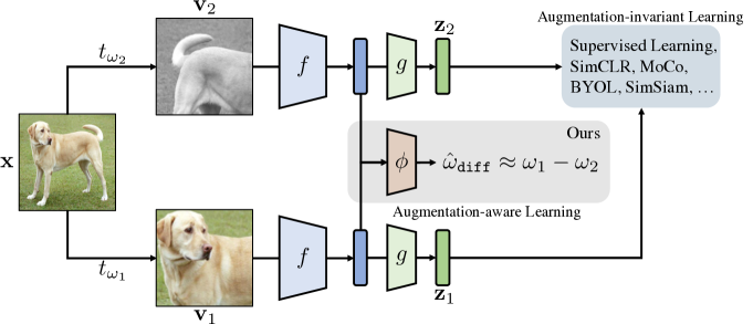
Figure 1: Illustration of the proposed method, AugSelf, that learns augmentation-aware information by predicting the difference between two augmentation parameters $\omega_{1}$ and $\omega_{2}$. Here, $\mathbf{x}$ is an original image, $\mathbf{v}=t_{\omega}(\mathbf{x})$ is an augmented sample by an augmentation $t_{\omega}$, $f$ is a feature extractor such as ResNet [20], and $g$ is a classifier for supervised learning or a projection MLP head for the recent unsupervised learning methods [1, 2, 12, 13].

Contribution. We first found that learning representations with an augmentation-invariant objective might hurt its performance in downstream tasks that rely on information related to the augmentations. For example, learning invariance against strong color augmentations forces the representations to contain less color information (see Figure 2(a)). Hence, it degrades the performance of the representations in color-sensitive downstream tasks such as the Flowers classification task [21] (see Figure 2(b)).

To prevent this information loss and obtain more generalizable representations, we propose an auxiliary self-supervised loss, coined AugSelf, that learns the difference of augmentation parameters between the two augmented samples (or views) as shown in Figure 1. For example, in the case of random cropping, AugSelf learns to predict the difference of cropping positions of two randomly cropped views. We found that AugSelf encourages the self-supervised representation learning methods, such as SimCLR [2] and SimSiam [13], to preserve augmentation-aware information (see Figure 2(a)) that could be useful for downstream tasks. Furthermore, AugSelf can easily be incorporated into the recent unsupervised representation learning methods [1, 2, 12, 13] with a negligible additional training cost, which is for training an auxiliary prediction head $\phi$ in Figure 1.

Somewhat interestingly, we also found that optimizing the auxiliary loss, AugSelf, can even improve the transferability of representations learned under the standard supervised representation learning scenarios [22]. This is because supervised learning also forces invariance, i.e., assigns the same label, for all augmented samples (of the same instance), and AugSelf can help to keep augmentation-aware knowledge in the learned representations.

We demonstrate the effectiveness of AugSelf under extensive transfer learning experiments: AugSelf improves (a) two unsupervised representation learning methods, MoCo [1] and SimSiam [13], in 20 of 22 tested scenarios; (b) supervised pretraining in 9 of 11 (see Table 1). Furthermore, we found that AugSelf is also effective under few-shot learning setups (see Table 2).

Remark that learning augmentation-invariant representations has been a common practice for both supervised and unsupervised representation learning frameworks, while the importance of augmentation-awareness is less emphasized. We hope that our work could inspire researchers to rethink the under-explored aspect and provide a new angle in representation learning.

2 Preliminaries: Augmentation-invariant representation learning

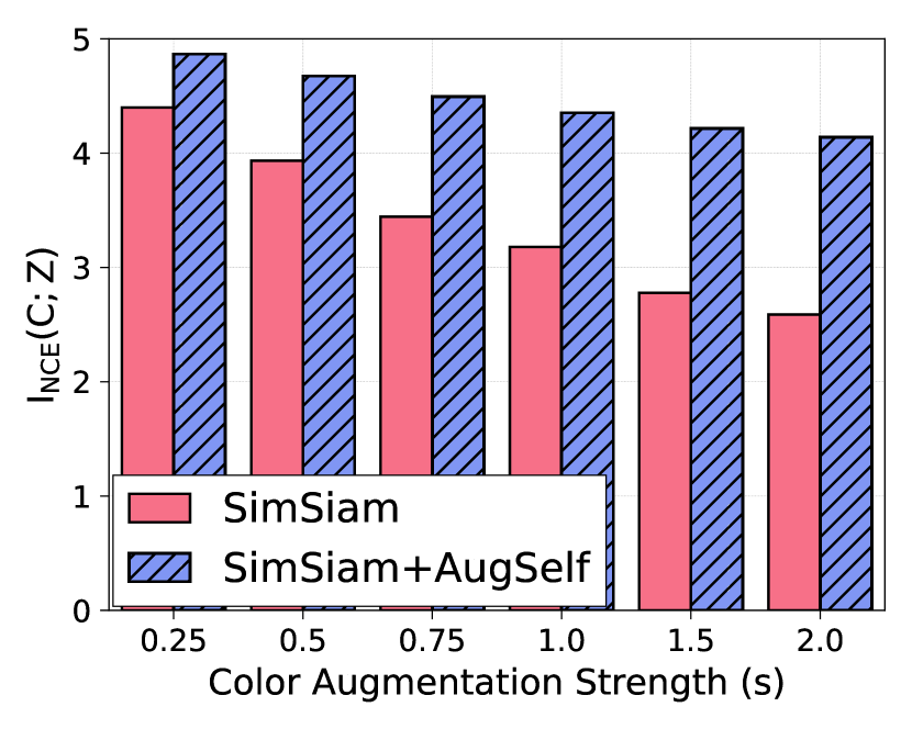
(a) Mutual information

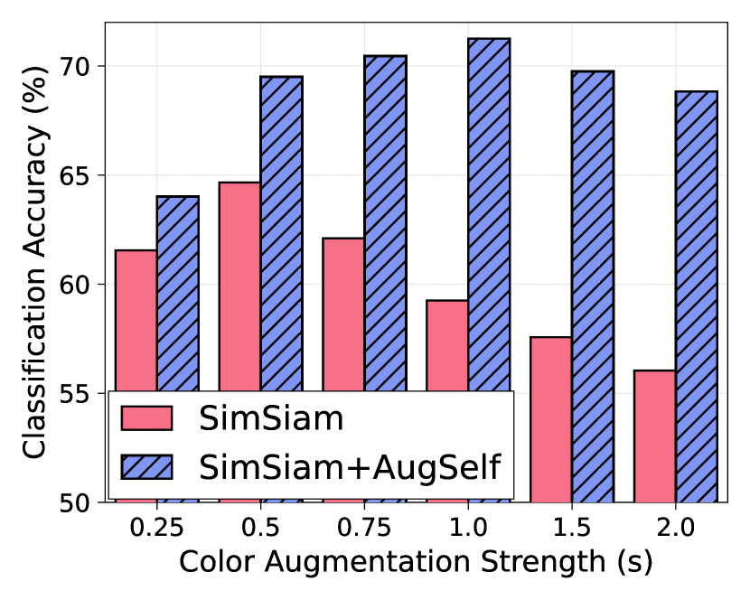
(b) STL10$\rightarrow$Flowers

(c) STL10$\rightarrow$Food

Figure 2: (a) Changes of mutual information, i.e., $I_{\tt NCE}(C;\mathbf{z})$, between color information $C(\mathbf{x})$ and the representation $\mathbf{z}=f(\mathbf{x})$ pretrained on STL10 [23] with varying the color jittering strength $s$. The pretrained representations are evaluated in color-sensitive benchmarks, (b) Flowers [21] and (c) Food [24], by the linear evaluation protocol [25].

In this section, we review the recent unsupervised representation learning methods [1, 2, 11, 12, 13] that learn representations by optimizing augmentation-invariant objectives. Formally, let $\mathbf{x}$ be an image, $t_{\omega}$ be an augmentation function parameterized by an augmentation parameter $\omega$, $\mathbf{v}=t_{\omega}(\mathbf{x})$ be the augmented sample (or view) of $\mathbf{x}$ by $t_{\omega}$, and $f$ be a CNN feature extractor, such as ResNet [20]. Generally speaking, the methods encourage the representations $f(\mathbf{v}_{1})$ and $f(\mathbf{v}_{2})$ to be invariant to the two randomly augmented views $\mathbf{v}_{1}=t_{\omega_{1}}(\mathbf{x})$ and $\mathbf{v}_{2}=t_{\omega_{2}}(\mathbf{x})$, i.e., $f(\mathbf{v}_{1})\approx f(\mathbf{v}_{2})$ for $\omega_{1},\omega_{2}\sim\Omega$ where $\Omega$ is a pre-defined augmentation parameter distribution. We now describe the recent methods one by one briefly. For simplicity, we here omit the projection MLP head $g(\cdot)$ which is widely used in the methods (see Figure 1).

Instance contrastive learning approaches [1, 2, 26] minimize the distance between an anchor $f(t_{\omega_{1}}(\mathbf{x}))$ and its positive sample $f(t_{\omega_{2}}(\mathbf{x}))$, while maximizing the distance between the anchor $f(t_{\omega_{1}}(\mathbf{x}))$ and its negative sample $f(t_{\omega_{3}}(\mathbf{x}^{\prime}))$. Since contrastive learning performance depends on the number of negative samples, a memory bank [26], a large batch [2], or a momentum network with a representation queue [1] has been utilized.

Clustering approaches [11, 27, 28] encourage two representations $f(t_{\omega_{1}}(\mathbf{x}))$ and $f(t_{\omega_{2}}(\mathbf{x}))$ to be assigned into the same cluster, in other words, the distance between them will be minimized.

Negative-free methods [12, 13] learn to predict the representation $f(\mathbf{v}_{1})$ of a view $\mathbf{v}_{1}=t_{\omega_{1}}(\mathbf{x})$ from another view $\mathbf{v}_{2}=t_{\omega_{2}}(\mathbf{x})$. For example, SimSiam [13] minimizes $\lVert h(f(\mathbf{v}_{2}))-\mathtt{sg}(f(\mathbf{v}_{1}))\rVert_{2}^{2}$ where $h$ is an MLP and $\mathtt{sg}$ is the stop-gradient operation. In these methods, if $h$ is optimal, then $h(f(\mathbf{v}_{2}))=\mathbb{E}_{\omega_{1}\sim\Omega}[f(\mathbf{v_{1}})]$; thus, the expectation of the objective can be rewritten as $\mathrm{Var}_{\omega\sim\Omega}(f(\mathbf{v}))$. Therefore, the methods can be considered as learning invariance with respect to the augmentations.

Supervised learning approaches [22] also learn augmentation-invariant representations. Since they often maximize $\exp(\mathbf{c}^{\top}_{y}f(t(\mathbf{x})))/\sum_{y^{\prime}}\exp(\mathbf{c}^{\top}_{y^{\prime}}f(t(\mathbf{x})))$ where $\mathbf{c}_{y}$ is the prototype vector of the label $y$, $f(t(\mathbf{x}))$ is concentrated to $\mathbf{c}_{y}$, i.e., $\mathbf{c}_{y}\approx f(t_{\omega_{1}}(\mathbf{x}))\approx f(t_{\omega_{2}}(\mathbf{x}))$.

These approaches encourage representations $f(\mathbf{x})$ to contain shared (i.e., augmentation-invariant) information between $t_{\omega_{1}}(\mathbf{x})$ and $t_{\omega_{2}}(\mathbf{x})$ and discard other information [15]. For example, if $t_{\omega}$ changes color information, then to satisfy $f(t_{\omega_{1}}(\mathbf{x}))=f(t_{\omega_{2}}(\mathbf{x}))$ for any $\omega_{1},\omega_{2}\sim\Omega$, $f(\mathbf{x})$ will be learned to contain no (or less) color information. To verify this, we pretrain ResNet-18 [20] on STL10 [29] using SimSiam [13] with varying the strength $s$ of the color jittering augmentation. To measure the mutual information between representations and color information, we use the InfoNCE loss [30]. We here simply encode color information as RGB color histograms of an image. As shown in Figure 2(a), using stronger color augmentations leads to color-relevant information loss. In classification on Flowers [21] and Food [24], which is color-sensitive, the learned representations containing less color information result in lower performance as shown in Figure 2(b) and 2(c), respectively. This observation emphasizes the importance of learning augmentation-aware information in transfer learning scenarios.

3 Auxiliary augmentation-aware self-supervision

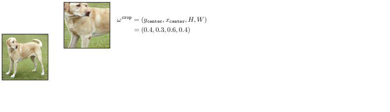
Figure 3: Examples of the commonly-used augmentations and their parameters $\omega^{\mathtt{aug}}$.

In this section, we introduce auxiliary augmentation-aware self-supervision, coined AugSelf, which encourages to preserve augmentation-aware information for generalizable representation learning. To be specific, we add an auxiliary self-supervision loss, which learns to predict the difference between augmentation parameters of two randomly augmented views, into existing augmentation-invariant representation learning methods [1, 2, 11, 12, 13]. We first describe a general form of our auxiliary loss, and then specific forms for various augmentations. For conciseness, let $\theta$ be the collection of all parameters in the model.

Since an augmentation function $t_{\omega}$ is typically a composition of different types of augmentations, the augmentation parameter $\omega$ can be written as $\omega=(\omega^{\mathtt{aug}})_{\mathtt{aug}\in\mathcal{A}}$ where $\mathcal{A}$ is the set of augmentations used in pretraining (e.g., $\mathcal{A}=\{\mathtt{crop},\mathtt{flip}$}), and $\omega^{\mathtt{aug}}$ is an augmentation-specific parameter (e.g., $\omega^{\mathtt{crop}}$ decides how to crop an image). Then, given two randomly augmented views $\mathbf{v}_{1}=t_{\omega_{1}}(\mathbf{x})$ and $\mathbf{v}_{2}=t_{\omega_{2}}(\mathbf{x})$, the AugSelf objective is as follows:

$$\mathcal{L}_{\mathtt{AugSelf}}(\mathbf{x},\omega_{1},\omega_{2};\theta)=\sum\nolimits_{\mathtt{aug}\in\mathcal{A}_{\mathtt{AugSelf}}}\mathcal{L}_{\mathtt{aug}}\big{(}\phi_{\theta}^{\mathtt{aug}}(f_{\theta}(\mathbf{v}_{1}),f_{\theta}(\mathbf{v}_{2})),\omega^{\mathtt{aug}}_{\mathtt{diff}}\big{)},$$

where $\mathcal{A}_{\mathtt{AugSelf}}\subseteq\mathcal{A}$ is the set of augmentations for augmentation-aware learning, $\omega^{\mathtt{aug}}_{\mathtt{diff}}$ is the difference between two augmentation-specific parameters $\omega_{1}^{\mathtt{aug}}$ and $\omega_{2}^{\mathtt{aug}}$, $\mathcal{L}_{\mathtt{aug}}$ is an augmentation-specific loss, and $\phi_{\theta}^{\mathtt{aug}}$ is a 3-layer MLP for $\omega_{\mathtt{diff}}^{\mathtt{aug}}$ prediction. This design allows us to incorporate AugSelf into the recent state-of-the-art unsupervised learning methods [1, 2, 11, 12, 13] with a negligible additional training cost. For example, the objective of SimSiam [13] with AugSelf can be written as $\mathcal{L}_{\mathtt{total}}(\mathbf{x},\omega_{1},\omega_{2};\theta)=\mathcal{L}_{\mathtt{SimSiam}}(\mathbf{x},\omega_{1},\omega_{2};\theta)+\lambda\cdot\mathcal{L}_{\mathtt{AugSelf}}(\mathbf{x},\omega_{1},\omega_{2};\theta),$ where $\lambda$ is a hyperparameter for balancing losses. Remark that the total objective $\mathcal{L}_{\mathtt{total}}$ encourages the shared representation $f(\mathbf{x})$ to learn both augmentation-invariant and augmentation-aware features. Hence, the learned representation $f(\mathbf{x})$ also can be useful in various downstream (e.g., augmentation-sensitive) tasks.

In this paper, we mainly focus on the commonly-used augmentations in the recent unsupervised representation learning methods [1, 2, 11, 12, 13]: random cropping, random horizontal flipping, color jittering, and Gaussian blurring; however, we remark that different types of augmentations can be incorporated into AugSelf (see Section 4.2). In the following, we elaborate on the details of $\omega^{\mathtt{aug}}$ and $\mathcal{L}_{\mathtt{aug}}$ for each augmentation. The examples of $\omega^{\mathtt{aug}}$ are illustrated in Figure 3.

Random cropping. The random cropping is the most popular augmentation in vision tasks. A cropping parameter $\omega^{\mathtt{crop}}$ contains the center position and cropping size. We normalize the values by the height and width of the original image $\mathbf{x}$, i.e., $\omega^{\mathtt{crop}}\in[0,1]^{4}$. Then, we use $\ell_{2}$ loss for $\mathcal{L}_{\mathtt{crop}}$ and set $\omega_{\mathtt{diff}}^{\mathtt{crop}}=\omega^{\mathtt{crop}}_{1}-\omega^{\mathtt{crop}}_{2}$.

Random horizontal flipping. A flipping parameter $\omega^{\mathtt{flip}}\in\{0,1\}$ indicates the image is horizontally flipped or not. Since it is discrete, we use the binary cross-entropy loss for $\mathcal{L}_{\mathtt{flip}}$ and set $\omega_{\mathtt{diff}}^{\mathtt{flip}}=\mathbbm{1}[{\omega^{\mathtt{flip}}_{1}=\omega^{\mathtt{flip}}_{2}}]$.

Color jittering. The color jittering augmentation adjusts brightness, contrast, saturation, and hue of an input image in a random order. For each adjustment, its intensity is uniformly sampled from a pre-defined interval. We normalize all intensities into $[0,1]$, i.e., $\omega^{\mathtt{color}}\in[0,1]^{4}$. Similarly to cropping, we use $\ell_{2}$ loss for $\mathcal{L}_{\mathtt{color}}$ and set $\omega^{\mathtt{color}}_{\mathtt{diff}}=\omega^{\mathtt{color}}_{1}{-}\omega^{\mathtt{color}}_{2}$.

Gaussian blurring. This blurring operation is widely used in unsupervised representation learning. The Gaussian filter is constructed by a single parameter, standard deviation $\sigma=\omega^{\mathtt{blur}}$. We also normalize the parameter into $[0,1]$. Then, we use $\ell_{2}$ loss for $\mathcal{L}_{\mathtt{blur}}$ and set $\omega^{\mathtt{blur}}_{\mathtt{diff}}=\omega^{\mathtt{blur}}_{1}{-}\omega^{\mathtt{blur}}_{2}$.

4 Experiments

Setup. We pretrain the standard ResNet-18 [20] and ResNet-50 on STL10 [23] and ImageNet100 [31, 32], respectively. We use two recent unsupervised representation learning methods as baselines for pretraining: a contrastive method, MoCo v2 [1, 14], and a non-contrastive method, SimSiam [13]. For STL10 and ImageNet100, we pretrain networks for $200$ and $500$ epochs with a batch size of $256$, respectively. For supervised pretraining, we pretrain ResNet-50 for $100$ epochs with a batch size of $128$ on ImageNet100. For augmentations, we use random cropping, flipping, color jittering, grayscaling, and Gaussian blurring following Chen and He [13]. In this section, our AugSelf predicts random cropping and color jittering parameters, i.e., $\mathcal{A}_{\mathtt{AugSelf}}=\{\mathtt{crop},\mathtt{color}\}$, unless otherwise stated. We set $\lambda=1.0$ for STL10 and $\lambda=0.5$ for ImageNet100. The other details and the sensitivity analysis to the hyperparameter $\lambda$ are provided in Appendix F and B, respectively. For ablation study (Section 4.2), we only use STL10-pretrained models.

Table 1: Linear evaluation accuracy (%) of ResNet-50 [20] and ResNet-18 pretrained on ImageNet100 [31, 32] and STL10 [23], respectively. Bold entries are the best of each baseline.

Method	CIFAR10	CIFAR100	Food	MIT67	Pets	Flowers	Caltech101	Cars	Aircraft	DTD	SUN397
ImageNet100-pretrained ResNet-50
SimSiam	86.89	66.33	61.48	65.75	74.69	88.06	84.13	48.20	48.63	65.11	50.60
+ AugSelf (ours)	88.80	70.27	65.63	67.76	76.34	90.70	85.30	47.52	49.76	67.29	52.28
MoCo v2	84.60	61.60	59.37	61.64	70.08	82.43	77.25	33.86	41.21	64.47	46.50
+ AugSelf (ours)	85.26	63.90	60.78	63.36	73.46	85.70	78.93	37.35	39.47	66.22	48.52
Supervised	86.16	62.70	53.89	52.91	73.50	76.09	77.53	30.61	36.78	61.91	40.59
+ AugSelf (ours)	86.06	63.77	55.84	54.63	74.81	78.22	77.47	31.26	38.02	62.07	41.49
STL10-pretrained ResNet-18
SimSiam	82.35	54.90	33.99	39.15	44.90	59.19	66.33	16.85	26.06	42.57	29.05
+ AugSelf (ours)	82.76	58.65	41.58	45.67	48.42	72.18	72.75	21.17	33.17	47.02	34.14
MoCo v2	81.18	53.75	33.69	39.01	42.34	61.01	64.15	16.09	26.63	41.20	28.50
+ AugSelf (ours)	82.45	57.17	36.91	41.67	43.80	66.96	66.02	17.53	28.02	45.21	30.93

4.1 Main results

Table 2: Few-shot classification accuracy (%) with 95% confidence intervals averaged over 2000 episodes on FC100 [33], CUB200 [34], and Plant Disease [35]. $(N,K)$ denotes $N$-way $K$-shot tasks. Bold entries are the best of each group.

	FC100		CUB200		Plant Disease
Method	(5, 1)	(5, 5)	(5, 1)	(5, 5)	(5, 1)	(5, 5)
ImageNet100-pretrained ResNet-50
SimSiam	36.19±0.36	50.36±0.38	45.56±0.47	62.48±0.48	75.72±0.46	89.94±0.31
+ AugSelf (ours)	39.37±0.40	55.27±0.38	48.08±0.47	66.27±0.46	77.93±0.46	91.52±0.29
MoCo v2	31.67±0.33	43.88±0.38	41.67±0.47	56.92±0.47	65.73±0.49	84.98±0.36
+ AugSelf (ours)	35.02±0.36	48.77±0.39	44.17±0.48	57.35±0.48	71.80±0.47	87.81±0.33
Supervised	33.15±0.33	46.59±0.37	46.57±0.48	63.69±0.46	68.95±0.47	88.77±0.30
+ AugSelf (ours)	34.70±0.35	48.89±0.38	47.58±0.48	65.31±0.45	70.82±0.46	89.77±0.29
STL10-pretrained ResNet-18
SimSiam	36.72±0.35	51.49±0.36	37.97±0.43	50.61±0.45	58.13±0.50	75.98±0.40
+ AugSelf (ours)	40.68±0.39	56.26±0.38	41.60±0.42	56.33±0.44	62.85±0.49	81.14±0.37
MoCo v2	35.69±0.34	49.26±0.36	37.62±0.42	50.71±0.44	57.87±0.48	75.98±0.40
+ AugSelf (ours)	39.66±0.39	55.58±0.39	38.33±0.41	51.93±0.44	60.78±0.50	78.76±0.38

Linear evaluation in various downstream tasks. We evaluate the pretrained networks in downstream classification tasks on 11 datasets: CIFAR10/100 [29], Food [24], MIT67 [36], Pets [37], Flowers [21], Caltech101 [38], Cars [39], Aircraft [40], DTD [41], and SUN397 [42]. They contain roughly 1k$\sim$70k training images. We follow the linear evaluation protocol [25]. The detailed information of datasets and experimental settings are described in Appendix E and G, respectively. Table 1 shows the transfer learning results in the various downstream tasks. Our AugSelf consistently improves (a) the recent unsupervised representation learning methods, SimSiam [13] and MoCo [13], in 10 out of 11 downstream tasks; and (b) supervised pretraining in 9 out of 11 downstream tasks. These consistent improvements imply that our method encourages to learn more generalizable representations.

Few-shot classification. We also evaluate the pretrained networks on various few-shot learning benchmarks: FC100 [33], Caltech-UCSD Birds (CUB200) [43], and Plant Disease [35]. Note that CUB200 and Plant Disease benchmarks require low-level features such as color information of birds and leaves, respectively, to detect their fine-grained labels. They are widely used in cross-domain few-shot settings [44, 45]. For few-shot learning, we perform logistic regression using the frozen representations $f(\mathbf{x})$ without fine-tuning. Table 2 shows the few-shot learning performance of 5-way 1-shot and 5-way 5-shot tasks. As shown in the table, our AugSelf improves the performance of SimSiam [13] and MoCo [1] in all cases with a large margin. For example, for plant disease detection [35], we obtain up to 6.07% accuracy gain in 5-way 1-shot tasks. These results show that our method is also effective in such transfer learning scenarios.

Comparison with LooC. Recently, Xiao et al. [16] propose LooC that learns augmentation-aware representations via multiple augmentation-specific contrastive learning objectives. Table 3 shows head-to-head comparisons under the same evaluation setup following Xiao et al. [16]. As shown in the table, our AugSelf has two advantages over LooC: (a) AugSelf requires the same number of augmented samples compared to the baseline unsupervised representation learning methods while LooC requires more, such that AugSelf does not increase the computational cost; (b) AugSelf can be incorporated with non-contrastive methods e.g., SimSiam [13], and SimSiam with AugSelf outperforms LooC in all cases.

Table 3: Linear evaluation accuracy (%) under the same setup following Xiao et al. [16]. The augmentations in the brackets of LooC [16] indicate which augmentation-aware information is learned. $N$ is the number of required augmented samples for each instance, that reflects the effective training batch size. ^∗ indicates that the numbers are reported in [16]. The numbers in the brackets show the accuracy gains compared to each baseline.

Method	$N$	ImageNet100	CUB200	Flowers (5-shot)	Flowers (10-shot)
MoCo∗ [1]	2	81.0	36.7	67.9±0.5	77.3±0.1
LooC∗ [16] (color)	3	81.1 (+0.1)	40.1 (+3.4)	68.2±0.6 (+0.3)	77.6±0.1 (+0.3)
LooC∗ [16] (rotation)	3	80.2 (-0.8)	38.8 (+2.1)	70.1±0.4 (+2.2)	79.3±0.1 (+2.0)
LooC∗ [16] (color, rotation)	4	79.2 (-1.8)	39.6 (+2.9)	70.9±0.3 (+3.0)	80.8±0.2 (+3.5)
MoCo [1]	2	81.0	32.2	78.5±0.3	81.2±0.3
MoCo [1] + AugSelf (ours)	2	82.4 (+1.4)	37.0 (+4.8)	81.7±0.2 (+3.2)	84.5±0.2 (+3.3)
SimSiam [13]	2	81.6	38.4	83.6±0.3	85.9±0.2
SimSiam [13] + AugSelf (ours)	2	82.6 (+1.0)	45.3 (+6.9)	86.4±0.2 (+2.8)	88.3±0.1 (+2.4)

Method	Error
SimSiam	0.00462
+ AugSelf (ours)	0.00335
MoCo	0.00487
+ AugSelf (ours)	0.00429
Supervised	0.00520
+ AugSelf (ours)	0.00473

Table 4: $\ell_{2}$ errors of bounding box predictions on CUB200.

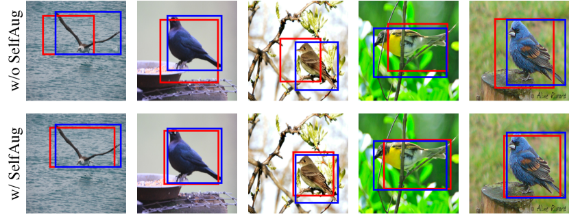
Figure 4: Examples of bounding box predictions on CUB200. Blue and red boxes are ground-truth and model prediction, respectively.

Object localization. We also evaluate representations in an object localization task (i.e., bounding box prediction) that requires positional information. We experiment on CUB200 [46] and solve linear regression using representations pretrained by SimSiam [13] without or with our method. Table 4 reports $\ell_{2}$ errors of bounding box predictions and Figure 4 shows the examples of the predictions. These results demonstrate that AugSelf is capable of learning positional information.

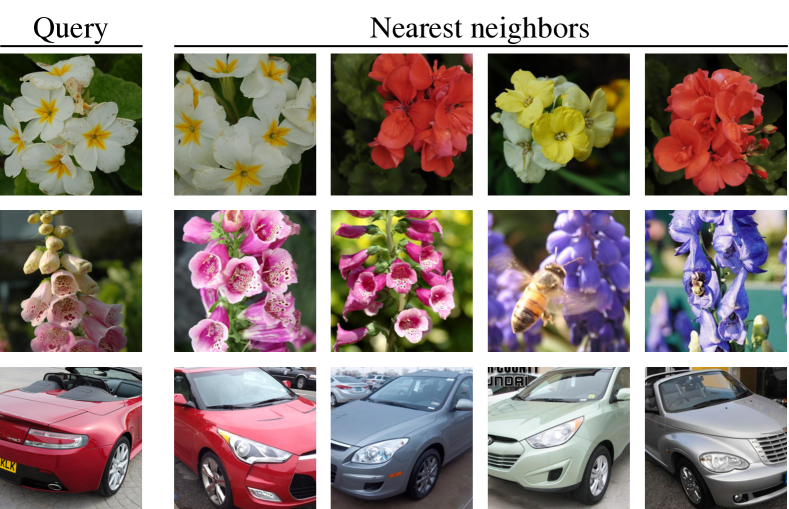
(a) SimSiam

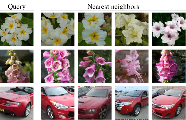
(b) SimSiam + AugSelf (ours)

Figure 5: Top-4 nearest neighbors based on the cosine similarity using representations $f(\mathbf{x})$ learned by (a) SimSiam [13] or (b) SimSiam with AugSelf (ours).

Retrieval. Figure 5 shows the retrieval results using pretrained models. For this experiment, we use the Flowers [21] and Cars [39] datasets and find top-4 nearest neighbors based on the cosine similarity between representations $f(\mathbf{x})$ where $f$ is the pretrained ResNet-50 on ImageNet100. As shown in the figure, the representations learned by AugSelf are more color-sensitive.

4.2 Ablation study

Table 5: Linear evaluation accuracy (%) of ResNet-18 [20] pretrained by each augmentation prediction task without other methods such as SimSiam [13]. We report SimSiam [13] results as reference. Bold entries are larger than the random initialization.

Pretraining objective	STL10	CIFAR10	CIFAR100	Food	MIT67	Pets	Flowers
Random Init	42.72	47.45	23.73	11.54	12.29	12.94	26.06
$\mathcal{L}_{\mathtt{crop}}$	68.28	70.78	43.44	22.26	26.17	27.68	38.21
$\mathcal{L}_{\mathtt{flip}}$	46.45	53.80	24.89	9.69	11.99	10.71	13.04
$\mathcal{L}_{\mathtt{color}}$	61.14	63.39	40.38	28.02	25.35	24.49	54.42
$\mathcal{L}_{\mathtt{blur}}$	48.26	46.60	20.44	8.73	11.87	13.07	17.20
SimSiam [13]	85.19	82.35	54.90	33.99	39.15	44.90	59.19

Table 6: Linear evaluation accuracy (%) of ResNet-18 [20] pretrained by SimSiam [13] with various combinations of our augmentation prediction tasks. Bold entries are the best of each task.

$\mathcal{A}_{\mathtt{AugSelf}}$	STL10	CIFAR10	CIFAR100	Food	MIT67	Pets	Flowers
$\emptyset$	85.19	82.35	54.90	33.99	39.15	44.90	59.19
$\{\mathtt{crop}\}$	85.98	82.82	55.78	35.68	43.21	47.10	62.05
$\{\mathtt{color}\}$	85.55	82.90	58.11	40.32	43.56	47.85	71.08
$\{\mathtt{crop},\mathtt{color}\}$	85.70	82.76	58.65	41.58	45.67	48.42	72.18

Effect of augmentation prediction tasks. We first evaluate the proposed augmentation prediction tasks one by one without incorporating invariance-learning methods. More specifically, we pretrain $f_{\theta}$ using only $\mathcal{L}_{\mathtt{aug}}$ for each $\mathtt{aug}\in\{\mathtt{crop},\mathtt{flip},\mathtt{color},\mathtt{blur}\}$. Remark that training objectives are different but we use the same set of augmentations. Table 5 shows the transfer learning results in various downstream tasks. We observe that solving horizontal flipping and Gaussian blurring prediction tasks results in worse or similar performance to a random initialized network in various downstream tasks, i.e., the augmentations do not contain task-relevant information. However, solving random cropping and color jittering prediction tasks significantly outperforms the random initialization in all downstream tasks. Furthermore, surprisingly, the color jittering prediction task achieves competitive performance in the Flowers [21] dataset compared to a recent state-of-the-art method, SimSiam [13]. These results show that augmentation-aware information are task-relevant and learning such information could be important in downstream tasks.

Based on the above observations, we incorporate random cropping and color jittering prediction tasks into SimSiam [13] when pretraining. More specifically, we optimize $\mathcal{L}_{\mathtt{SimSiam}}+\lambda_{\mathtt{crop}}\mathcal{L}_{\mathtt{crop}}+\lambda_{\mathtt{color}}\mathcal{L}_{\mathtt{color}}$ where $\lambda_{\mathtt{crop}},\lambda_{\mathtt{color}}\in\{0,1\}$. The transfer learning results are reported in Table 6. As shown in the table, each self-supervision task improves SimSiam consistently (and often significantly) in various downstream tasks. For example, the color jittering prediction task improves SimSiam by 6.33% and 11.89% in Food [24] and Flowers [21] benchmarks, respectively. When incorporating both tasks simultaneously, we achieve further improvements in almost all the downstream tasks. Furthermore, as shown in Figure 2, our AugSelf preserves augmentation-aware information as much as possible; hence our gain is consistent regardless of the strength of color jittering augmentation.

Table 7: Transfer learning accuracy (%) of ResNet-18 [20] pretrained by SimSiam [13] with or without our AugSelf using strong augmentations. $\mathtt{C}$, $\mathtt{J}$, $\mathtt{R}$ and $\mathtt{S}$ denote cropping, color jittering, rotation and solarization prediction tasks, respectively. Bold entries are the best of each augmentation.

Strong Aug.	$\mathcal{A}_{\mathtt{AugSelf}}$	STL10	CIFAR10	CIFAR100	Food	MIT67	Pets	Flowers
None	$\emptyset$	85.19	82.35	54.90	33.99	39.15	44.90	59.19
	$\{\mathtt{C},\mathtt{J}\}$	85.70	82.76	58.65	41.58	45.67	48.42	72.18
Rotation	$\emptyset$	80.11	77.78	50.24	36.40	36.39	41.43	61.77
	$\{\mathtt{C},\mathtt{J}\}$	81.85	79.93	57.27	43.04	41.32	47.30	72.52
	$\{\mathtt{C},\mathtt{J},\mathtt{R}\}$	82.67	80.71	58.28	43.28	44.48	46.65	72.94
Solarization	$\emptyset$	86.32	81.08	52.50	32.59	41.29	44.76	58.79
	$\{\mathtt{C},\mathtt{J}\}$	86.03	82.64	57.94	40.29	46.67	48.81	71.43
	$\{\mathtt{C},\mathtt{J},\mathtt{S}\}$	85.91	82.63	58.18	40.17	45.57	49.02	71.43

Different augmentations. We confirm that our method can allow to use other strong augmentations: rotation, which rotates an image by $0^{\circ}$, $90^{\circ}$, $180^{\circ}$, $270^{\circ}$ degrees randomly; and solarization, which inverts each pixel value when the value is larger than a randomly sampled threshold. Based on the default augmentation setting, i.e., $\mathcal{A}_{\mathtt{AugSelf}}=\{\mathtt{crop},\mathtt{color}\}$, we additionally apply each augmentation with a probability of $0.5$. We also evaluate the effectiveness of augmentation prediction tasks for rotation and solarization. Note that we formulate the rotation prediction as a 4-way classification task (i.e., $\omega^{\mathtt{rot}}_{\mathtt{diff}}\in\{0,1,2,3\}$) and the solarization prediction as a regression task (i.e., $\omega^{\mathtt{sol}}_{\mathtt{diff}}\in[-1,1]$). As shown in Table 7, we obtain consistent gains across various downstream tasks even if stronger augmentations are applied. Furthermore, in the case of rotation, we observe that our augmentation prediction task tries to prevent the performance degradation from learning invariance to rotations. For example, in CIFAR100 [29], the baseline loses 4.66% accuracy (54.90%$\rightarrow$50.24%) when using rotations, but ours does only 0.37% (58.65%$\rightarrow$58.28%). These results show that our AugSelf is less sensitive to the choice of augmentations. We believe that this robustness would be useful in future research on representation learning with strong augmentations.

Table 8: Linear evaluation accuracy in augmentation-aware pretext tasks.

Method	Rotation	Color perm
SimSiam	59.11	24.66
+ AugSelf	64.61	60.49

Solving geometric and color-related pretext tasks. To validate that our AugSelf is capable of learning augmentation-aware information, we try to solve two pretext tasks requiring the information: 4-way rotation ($0^{\circ}$, $90^{\circ}$, $180^{\circ}$, $270^{\circ}$) and 6-way color channel permutation (RGB, RBG, $\ldots$, BGR) classification tasks. We note that the baseline (SimSiam) and our method (SimSiam+AugSelf) do not observe rotated or color-permuted samples in the pretraining phase. We train a linear classifier on top of pretrained representation without finetuning for each task. As reported in Table 8, our AugSelf solves the pretext tasks well even without their prior knowledge in pretraining; these results validate that our method learns augmentation-aware information.

Compatibility with other methods. While we mainly focus on SimSiam [13] and MoCo [1] in the previous section, our AugSelf can be incorporated into other unsupervised learning methods, SimCLR [2], BYOL [12], and SwAV [11]. Table 9 shows the consistent and significant gains by AugSelf across all methods and downstream tasks.

Table 9: Transfer learning accuracy (%) of various unsupervised learning frameworks with and without our AugSelf framework. Bold entries indicates the best for each baseline method.

Method	AugSelf (ours)	STL10	CIFAR10	CIFAR100	Food	MIT67	Pets	Flowers
		84.87	78.93	48.94	31.97	36.82	43.18	56.20
SimCLR [2]	✓	84.99	80.92	53.64	36.21	40.62	46.51	64.31
		86.73	82.66	55.94	37.30	42.78	50.21	66.89
BYOL [12]	✓	86.79	83.60	59.66	42.89	46.17	52.45	74.07
		82.21	81.60	52.00	29.78	36.69	37.68	53.01
SwAV [11]	✓	82.57	82.00	55.10	33.16	39.13	40.74	61.69

5 Related work

Self-supervised pretext tasks. For visual representation learning without labels, various pretext tasks have been proposed in literature [17, 18, 19, 47, 48, 49, 50, 51] by constructing self-supervision from an image. For example, Doersch et al. [17], Noroozi and Favaro [18] split the original image $\mathbf{x}$ into $3\times 3$ patches and then learn visual representations by predicting relations between the patch locations. Instead, Zhang et al. [19], Larsson et al. [48] construct color prediction tasks by converting colorful images to gray ones. Zhang et al. [51] propose a similar task requiring to predict one subset of channels (e.g., depth) from another (e.g., RGB values). Meanwhile, Gidaris et al. [47], Qi et al. [49], Zhang et al. [50] show that solving affine transformation (e.g., rotation) prediction tasks can learn high-level representations. These approaches often require specific preprocessing procedures (e.g., $3\times 3$ patches [17, 18], or specific affine transformations [49, 50]). In contrast, our AugSelf can be working with common augmentations such as random cropping and color jittering. This advantage allows us to incorporate AugSelf to the recent state-of-the-art frameworks like SimCLR [2] while not increasing the computational cost. Furthermore, we emphasize that our contribution is not only to construct AugSelf, but also finding on the importance of learning augmentation-aware representations together with the existing augmentation-invariant approaches.

Augmentations for unsupervised representation learning. Chen et al. [2], Tian et al. [15] found that the choice of augmentations plays a critical role in contrastive learning. Based on this finding, many unsupervised learning methods [1, 2, 11, 12, 13] have used similar augmentations (e.g., cropping and color jittering) and then achieved outstanding performance in ImageNet [31]. Tian et al. [15] discuss a similar observation to ours that the optimal choice of augmentations is task-dependent, but they focus on finding the optimal choice for a specific downstream task. However, in the pretraining phase, prior knowledge of downstream tasks could be not available. In this case, we need to preserve augmentation-aware information in representations as much as possible for unknown downstream tasks. Recently, Xiao et al. [16] propose a contrastive method for learning augmentation-aware representations. This method requires additional augmented samples for each augmentation; hence, the training cost increases with respect to the number of augmentations. Furthermore, the method is specialized to contrastive learning only, and is not attractive to be used for non-contrastive methods like BYOL [12]. In contrast, our AugSelf does not suffer from these issues as shown in Table 3 and 9.

6 Discussion and conclusion

To improve the transferability of representations, we propose AugSelf, an auxiliary augmentation-aware self-supervision method that encourages representations to contain augmentation-aware information that could be useful in downstream tasks. Our idea is to learn to predict the difference between augmentation parameters of two randomly augmented views. Through extensive experiments, we demonstrate the effectiveness of AugSelf in various transfer learning scenarios. We believe that our work would guide many research directions for unsupervised representation learning and transfer learning.

Limitations. Even though our method provides large gains when we apply it to popular data augmentations like random cropping, it might not be applicable to some specific data augmentation, where it is non-trivial to parameterize augmentation such as GAN-based one [52]. Hence, an interesting future direction would be to develop an augmentation-agnostic way that does not require to explicitly design augmentation-specific self-supervision. Even for this direction, we think that our idea of learning the relation between two augmented samples could be used, e.g., constructing contrastive pairs between the relations.

Negative societal impacts. Self-supervised training typically requires a huge training cost (e.g., training MoCo v2 [14] for 1000 epochs requires 11 days on 8 V100 GPUs), a large network capacity (e.g., GPT3 [5] requires 175 billion parameters), therefore it raises environmental issues such as carbon generation [53]. Hence, efficient training methods [54] or distilling knowledge to a smaller network [55] would be required to ameliorate such environmental problems.

Appendix A Trade-off between augmentation invariance and awareness

We first emphasize that we want $f(\mathbf{x})$ to learn both augmentation-invariant and augmentation-aware information (or features) in the input $\mathbf{x}$. To this end, we train $g$ and $\phi$ to extract each information from $f(\mathbf{x})$, respectively; in other words, we want the functions $g(f(t_{1}(\mathbf{x})))$ and $\phi(f(t_{1}(\mathbf{x})),f(t_{2}(\mathbf{x})))$ to be invariant and variant with respect to the augmentation $t_{1}$ (and $t_{2}$), respectively. Here, if the shared network $f$ has a limited capacity (e.g., few parameters or dimension), the two training objectives (for $g$ and $\phi$) may interfere with each other, i.e., $f(\mathbf{x})$ might become less invariant (or contain less augmentation-invariant information). However, our choice $f$ of deep neural networks (DNNs) in our experiments does not suffer from the issue (i.e., DNNs are highly expressive), so our goal is achievable with a negligible loss of augmentation-invariant information. To support this, we compute the cosine similarity between representations from augmented and original samples, i.e., $\mathtt{CS}=\mathbb{E}_{\mathbf{x}\sim\mathcal{D},t\sim\mathcal{T}}[\mathtt{sim}(g\circ f(t(\mathbf{x})),g\circ f(\mathbf{x}))]$. Note that this metric becomes higher as the representation $g(f(\mathbf{x}))$ is more invariant to the augmentation $t\sim\mathcal{T}$. We here use STL10-pretrained models. Table 10 shows that AugSelf does not significantly change the cosine similarity $\mathtt{CS}$; in other words, AugSelf is not harmful to the augmentation-invariant objective.

Table 10: The invariance metric, $\mathtt{CS}=\mathbb{E}_{\mathbf{x}\sim\mathcal{D},t\sim\mathcal{T}}[\mathtt{sim}(g\circ f(t(\mathbf{x})),g\circ f(\mathbf{x}))]$, with 95% confidence intervals over 80k random samples in the STL10 test split [23]. Higher values mean $f(\mathbf{x})$ is more invariant to the augmentations $\mathcal{T}$.

AugSelf (ours)	SimSiam [13]	BYOL [12]	SimCLR [2]	MoCo [1]
	0.9263±0.0005	0.9555±0.0004	0.9378±0.0006	0.9274±0.0006
✓	0.9250±0.0006	0.9453±0.0004	0.9385±0.0005	0.9280±0.0006

Appendix B Hyperparameter sensitivity analysis

We simply use the same value of $\lambda$, e.g., $\lambda=1$ for STL10 experiments, across different augmentations and different downstream tasks. One can find a better hyperparameter by tuning it on each augmentation and each downstream task, but we do not make much effort to tune it as our method is not too sensitive to hyperparameters. We here provide the sensitivity analysis to the hyperparameter $\lambda$ with varying $\lambda\in\{0.5,1.0,2.0\}$ under the STL10 pretraining setup. Table 11 shows that the overall transfer learning performance is not too sensitive to $\lambda$ and AugSelf clearly improves the performance in all the cases over the baseline (i.e., $\lambda=0$).

Table 11: Linear evaluation accuracy (%) of ResNet-18 [20] pretrained by SimSiam [13] and our AugSelf with varying the hyperparameter $\lambda$.

Pretraining objective	$\lambda$	STL10	CIFAR10	CIFAR100	Food	MIT67	Pets	Flowers	Avg
$\mathcal{L}_{\mathtt{SimSiam}}$	$0.0$	85.19	82.35	54.90	33.99	39.15	44.90	59.19	57.09
$\mathcal{L}_{\mathtt{SimSiam}}+\lambda\mathcal{L}_{\mathtt{crop}}$	$0.5$	85.50	82.81	55.50	35.19	42.79	45.94	61.24	58.42
	$1.0$	85.98	82.82	55.78	35.68	43.21	47.10	62.05	58.95
	$2.0$	86.36	82.41	55.29	36.18	41.91	47.43	62.28	58.84
$\mathcal{L}_{\mathtt{SimSiam}}+\lambda\mathcal{L}_{\mathtt{color}}$	$0.5$	85.66	83.75	58.58	39.39	42.61	47.15	70.05	61.03
	$1.0$	85.55	82.90	58.11	40.32	43.56	47.85	71.08	61.34
	$2.0$	84.79	82.56	58.89	40.69	43.41	46.79	71.93	61.29
$\mathcal{L}_{\mathtt{SimSiam}}+\lambda(\mathcal{L}_{\mathtt{crop}}+\mathcal{L}_{\mathtt{color}})$	$0.5$	86.07	82.67	57.72	39.92	43.88	48.86	70.93	61.43
	$1.0$	85.70	82.76	58.65	41.58	45.67	48.42	72.18	62.14
	$2.0$	84.56	83.08	59.49	41.72	44.50	49.04	72.35	62.11

Appendix C Fine-tuning experiments

We fine-tune ImageNet100-pretrained models using a fine-tuning strategy, L2SP [56]. Following Xuhong et al. [56], we use the same set fo hyperparameters, i.e., $\beta=0.01$, $\alpha\in\{0.001,0.01,0.1,1\}$, and $lr\in\{0.005,0.01,0.02\}$. We evaluate the fine-tuning accuracy on five benchmarks, MIT67 [36], CUB200 [34], Food [24], Stanford Dogs [57], and Caltech256 [58]. Table 12 shows the effectiveness of our AugSelf in the fine-tuning scenarios.

Table 12: Fine-tuning accuracy (%) averaged over 5 trials with 95% confidence intervals.

Method	MIT67	CUB200	Food	Standford Dogs	Caltech256
SimSiam	67.69±0.48	67.59±0.41	66.66±0.36	69.34±0.29	52.37±0.45
+ AugSelf (ours)	69.31±0.56	70.22±0.66	70.19±0.18	70.26±0.20	54.66±0.07

Appendix D Robustness under perturbations

We also evaluate the robustness of the learned representations by our method. To this end, we use two types of robustness metrics: (1) adversarial robustness using the single-step fast gradient sign method (FGSM) [59] and (2) robustness to common corruptions, especially weather (fog, frost, and snow) corruptions, proposed by [60]. We here use supervised models trained on ImageNet100 for generating adversarial samples. Table 13 shows the classification accuracy on ImageNet100 under the two types of perturbations.

Table 13: Classification accuracy (%) under various perturbations.

		FGSM			Weather corruption
Method	Clean	$\epsilon=1/255$	$\epsilon=2/255$	$\epsilon=4/255$	Fog	Frost	Snow
SimSiam	85.60	32.48	22.80	17.70	57.53	53.96	43.85
+ AugSelf (ours)	85.40	32.90	21.60	16.64	57.42	53.97	45.65

We observe that our AugSelf does not significantly affect the robustness of learned representations. This result is somewhat interesting because the representations learned with AugSelf are more sensitive to diverse information than those without AugSelf. Since improving the adversarial robustness of self-supervised learning is an ongoing topic [61, 62], we believe that incorporating the idea with our framework would be an interesting research direction.

Appendix E Datasets

Table 14 summarizes detailed descriptions of (a) pretraining datasets, (c) linear evaluation benchmarks, and (c) few-shot learning benchmarks. For linear evaluation benchmarks, we randomly choose validation samples in the training split for each dataset when the validation split is not officially provided. For few-shot benchmarks, we use the meta-test split for FC100 [33], and whole datasets for CUB200 [34] and Plant Disease [35]. The evaluation details are described in Section G.

Table 14: Dataset information.

Category	Dataset	# of classes	Training	Validation	Test	Metric
(a) Pretraining	STL10 [23]	10	105000	-	-	-
	ImageNet100 [31, 32]	1000	126689	-	-	-
(b) Linear evaluation	STL10 [23]	10	4500	500	8000	Top-1 accuracy
	CIFAR10 [29]	10	45000	5000	10000	Top-1 accuracy
	CIFAR100 [29]	100	45000	5000	10000	Top-1 accuracy
	Food [24]	101	68175	7575	25250	Top-1 accuracy
	MIT67 [36]	67	4690	670	1340	Top-1 accuracy
	Pets [37]	37	2940	740	3669	Mean per-class accuracy
	Flowers [21]	102	1020	1020	6149	Mean per-class accuracy
	Caltech101 [38]	101	2525	505	5647	Mean Per-class accuracy
	Cars [39]	196	6494	1650	8041	Top-1 accuracy
	Aircraft [40]	100	3334	3333	3333	Mean Per-class accuracy
	DTD (split 1) [41]	47	1880	1880	1880	Top-1 accuracy
	SUN397 (split 1) [42]	397	15880	3970	19850	Top-1 accuracy
(c) Few-shot	FC100 [33]	20	-	-	12000	Average accuracy
	CUB200 [34]	200	-	-	11780	Average accuracy
	Plant Disease [35]	38	-	-	54305	Average accuracy

Appendix F Pretraining setup

F.1 ImageNet100 pretraining

We pretrain the standard ResNet-50 [20] architecture in the ImageNet100 [31, 32] dataset for $500$ training epochs using SimSiam [13] and MoCo [1] methods. We use a batch size of $256$ and a cosine learning rate schedule without restarts [63]. Note that the pretraining setups are the same as they officially used for ImageNet pretraining described in [13, 1, 14]. In multi-GPU experiments, we use the synchronized batch normalization following Chen and He [13]. When incorporating our AugSelf into the methods, we use $\lambda=0.5$ and $\mathcal{A}_{\mathtt{AugSelf}}=\{\mathtt{crop},\mathtt{color}\}$. Note that SimSiam [13] and MoCo [1] requires 32 and 29 hours on a single RTX3090 4-GPU machine, respectively.

SimSiam [13]. We use a learning rate $0.05$ and a weight decay of $0.0001$. We use a 3-layer projection MLP head $g(\cdot)$ with a hidden dimension of $2048$ and an output dimension of $2048$. We use a batch normalization [64] at the last layer in the projection MLP. We use a 2-layer prediction MLP head $h(\cdot)$ with a hidden dimension of $512$ and no batch normalization at the last layer in the prediction MLP. When optimizing the prediction MLP, we use a constant learning rate schedule following Chen and He [13].

MoCo [1]. We use a learning rate $0.03$ and a weight decay of $0.0001$. Following an advanced version of MoCo [14, MoCo v2], we use a 2-layer projection MLP head $g(\cdot)$ with a hidden dimension of 2048 and an output dimension of $128$. We use a batch normalization [64] at only the hidden layer. We also use a temperature scaling parameter of $0.2$, an exponential moving average parameter of $0.999$, and a queue size of $65536$.

F.2 STL10 pretraining

We pretrain the standard ResNet-18 [20] architecture in the STL10 [23] dataset. For all methods, we use the same optimization scheme: stochastic gradient descent (SGD) with a learning rate of $0.03$, a batch size of $256$, a weight decay of $0.0005$, a momentum of $0.9$. The learning rate follows a cosine decay schedule without restarts [63]. When incorporating our AugSelf into the methods, we use $\lambda=1.0$ and $\mathcal{A}_{\mathtt{AugSelf}}=\{\mathtt{crop},\mathtt{color}\}$, unless otherwise stated. We now describe method-specific hyperparameters one by one in the following.

SimCLR [2]. We use a 2-layer projection MLP head $g(\cdot)$ with a hidden dimension of $512$ and an output dimension of $128$. We do not use a batch normalization [64] at the last layer in the MLP. We use a temperature scaling parameter of $0.2$ in contrastive learning.

MoCo [1]. We use an advanced version of MoCo [14, MoCo v2] with the same projection MLP architecture as SimCLR used. Other hyperparameters are the same as the ImageNet100 setup described in Section F.1.

BYOL [12]. Following Grill et al. [12], we use a 2-layer projection MLP head $g(\cdot)$ with a hidden dimension of $4096$ and an output dimension of $256$. We do not use a batch normalization [64] at the last layer in the MLP. We use the same architecture for the prediction MLP head $h(\cdot)$. The exponential moving average parameter is increased starting from $0.996$ to $1.0$ with a cosine schedule following Grill et al. [12].

SimSiam [13]. We use a 2-layer projection MLP with a hidden dimension of $2048$ and an output dimension of $2048$. Other hyperparameters are the same as the ImageNet100 setup described in Section F.1.

SwAV [11]. We use a 2-layer projection MLP head $g(\cdot)$ with a hidden dimension of $2048$ and an output dimension of $128$ without batch normalization [64] at the last layer in the MLP. We use $100$ prototypes, a smoothness factor of $\epsilon=0.05$ and a temperature scaling parameter of $\tau=0.1$. We do not use the multi-resolution cropping technique and the additional queue storing previous batches for simplicity.

F.3 Augmentations

In this section, we describe augmentations using PyTorch [65] notations in the following. Note that we use random cropping, flipping, color jittering, grayscale, and Gaussian blurring unless otherwise stated.

• RandomResizedCrop. The scale of cropping is randomly sampled from $[0.2,1.0]$. The cropped images are resized to $96\times 96$ and $224\times 224$ for STL10 [23] and ImageNet [31] pretraining, respectively.

• RandomHorizontalFlip. This operation is randomly applied with a probability of $0.5$.

• ColorJitter. The maximum strengths of brightness, contrast, saturation and hue factors are $0.4$, $0.4$, $0.4$ and $0.1$, respectively. This operation is randomly applied with a probability of $0.8$. In Section 2, we adjust the strengths by multiplying a strength factor $s$, i.e., $s>1$ means stronger color jittering than the default configuration while $s<1$ means weaker color jittering.

• RandomGrayscale. This operation is randomly applied with a probability of $0.2$.

• GaussianBlur. The standard deviation is randomly sampled from $[0.1,2.0]$. The kernel size is $9\times 9$ and $23\times 23$ for STL10 [23] and ImageNet [31] pretraining, respectively. This operation is randomly applied with a probability of $0.5$.

• Rotation. This rotates an image by $0^{\circ},90^{\circ},180^{\circ},270^{\circ}$ randomly. This operation is randomly applied with a probability of $0.5$ after the default geometric augmentations are applied.

• Solarization. This inverts each pixel value when the value is larger than a randomly sampled threshold. Formally, for an uniformly sampled threshold $\delta\sim U(0,1)$,

  $$x_{\mathtt{new}}^{(i,j)}\leftarrow\mathbbm{1}[x_{\mathtt{old}}^{(i,j)}<\delta]x_{\mathtt{old}}^{(i,j)}+\mathbbm{1}[x_{\mathtt{old}}^{(i,j)}\geq\delta](1-x_{\mathtt{old}}^{(i,j)}),$$

  for all pixels $(i,j)$. This operation is randomly applied with a probability of $0.5$ right after ColorJitter is applied.

Appendix G Evaluation protocol

Linear evaluation benchmarks. We follow the same linear transfer evaluation protocol [2, 12, 25]; we train linear classifiers upon the frozen features extracted from $224\times 224$ (or $96\times 96$ for STL10 pretraining) center-cropped images without data augmentation. To be specific, images are first resized to $224$ pixels along the shorter side, and then cropped by $224\times 224$ at the center of the images. Then, we minimize the $\ell_{2}$-regularized cross-entropy objective using L-BFGS. The regularization parameter is selected from a range of 45 logarithmically spaced values from $10^{-6}$ to $10^{5}$ using the validation split. After selecting the best hyperparameter, we train again the linear classifier using both training and validation splits and then report the test accuracy using the model. Note that we set the maximum number of iterations in L-BFGS as $5000$ and use the previous solution as an initial point (i.e., warm start) for the next step.

Few-shot benchmarks. For evaluating representations in few-shot benchmarks, we simply perform logistic regression using the frozen representations $f(\mathbf{x})$ and $N{\times}K$ support samples without fine-tuning and data augmentation in a $N$-way $K$-shot episode.

Object localization. For predicting bounding box information (i.e., top left coordinates and sizes of bounding boxes), we simply perform linear regression⁷ using the frozen representations $f(\mathbf{x})$ and all training samples in CUB200 [34] without fine-tuning and data augmentation.

References

- He et al. [2020] Kaiming He, Haoqi Fan, Yuxin Wu, Saining Xie, and Ross Girshick. Momentum contrast for unsupervised visual representation learning. In Proceedings of the IEEE/CVF Conference on Computer Vision and Pattern Recognition, pages 9729–9738, 2020.
- Chen et al. [2020a] Ting Chen, Simon Kornblith, Mohammad Norouzi, and Geoffrey Hinton. A simple framework for contrastive learning of visual representations. In Proceedings of International Conference on Machine Learning, pages 1597–1607. PMLR, 2020a.
- Han et al. [2020] Tengda Han, Weidi Xie, and Andrew Zisserman. Self-supervised co-training for video representation learning. In Advances in Neural Information Processing Systems, 2020.
- Devlin et al. [2018] Jacob Devlin, Ming-Wei Chang, Kenton Lee, and Kristina Toutanova. Bert: Pre-training of deep bidirectional transformers for language understanding. arXiv preprint arXiv:1810.04805, 2018.
- Brown et al. [2020] Tom B Brown, Benjamin Mann, Nick Ryder, Melanie Subbiah, Jared Kaplan, Prafulla Dhariwal, Arvind Neelakantan, Pranav Shyam, Girish Sastry, Amanda Askell, et al. Language models are few-shot learners. In Advances in Neural Information Processing Systems, 2020.
- Feng et al. [2020] Zhangyin Feng, Daya Guo, Duyu Tang, Nan Duan, Xiaocheng Feng, Ming Gong, Linjun Shou, Bing Qin, Ting Liu, Daxin Jiang, et al. CodeBERT: A pre-trained model for programming and natural languages. In Proceedings of the Conference on Empirical Methods in Natural Language Processing: Findings, pages 1536–1547, 2020.
- Anand et al. [2019] Ankesh Anand, Evan Racah, Sherjil Ozair, Yoshua Bengio, Marc-Alexandre Côté, and R Devon Hjelm. Unsupervised state representation learning in atari. In Advances in Neural Information Processing Systems, pages 8769–8782, 2019.
- Stooke et al. [2021] Adam Stooke, Kimin Lee, Pieter Abbeel, and Michael Laskin. Decoupling representation learning from reinforcement learning. In Proceedings of International Conference on Machine Learning, 2021.
- Laskin et al. [2020] Michael Laskin, Aravind Srinivas, and Pieter Abbeel. CURL: Contrastive unsupervised representations for reinforcement learning. In Proceedings of International Conference on Machine Learning, pages 5639–5650, 2020.
- Hassani and Khasahmadi [2020] Kaveh Hassani and Amir Hosein Khasahmadi. Contrastive multi-view representation learning on graphs. In Proceedings of International Conference on Machine Learning, pages 4116–4126, 2020.
- Caron et al. [2020] Mathilde Caron, Ishan Misra, Julien Mairal, Priya Goyal, Piotr Bojanowski, and Armand Joulin. Unsupervised learning of visual features by contrasting cluster assignments. In Advances in Neural Information Processing Systems, 2020.
- Grill et al. [2020] Jean-Bastien Grill, Florian Strub, Florent Altché, Corentin Tallec, Pierre H Richemond, Elena Buchatskaya, Carl Doersch, Bernardo Avila Pires, Zhaohan Daniel Guo, Mohammad Gheshlaghi Azar, et al. Bootstrap Your Own Latent: A new approach to self-supervised learning. arXiv preprint arXiv:2006.07733, 2020.
- Chen and He [2020] Xinlei Chen and Kaiming He. Exploring simple siamese representation learning. arXiv preprint arXiv:2011.10566, 2020.
- Chen et al. [2020b] Xinlei Chen, Haoqi Fan, Ross Girshick, and Kaiming He. Improved baselines with momentum contrastive learning. arXiv preprint arXiv:2003.04297, 2020b.
- Tian et al. [2020] Yonglong Tian, Chen Sun, Ben Poole, Dilip Krishnan, Cordelia Schmid, and Phillip Isola. What makes for good views for contrastive learning? In Advances in Neural Information Processing Systems, pages 6827–6839, 2020.
- Xiao et al. [2021] Tete Xiao, Xiaolong Wang, Alexei A Efros, and Trevor Darrell. What should not be contrastive in contrastive learning. In International Conference on Learning Representations, 2021.
- Doersch et al. [2015] Carl Doersch, Abhinav Gupta, and Alexei A Efros. Unsupervised visual representation learning by context prediction. In Proceedings of the IEEE International Conference on Computer Vision, pages 1422–1430, 2015.
- Noroozi and Favaro [2016] Mehdi Noroozi and Paolo Favaro. Unsupervised learning of visual representations by solving jigsaw puzzles. In Proceedings of the European Conference on Computer Vision, pages 69–84. Springer, 2016.
- Zhang et al. [2016] Richard Zhang, Phillip Isola, and Alexei A Efros. Colorful image colorization. In Proceedings of the European Conference on Computer Vision, pages 649–666. Springer, 2016.
- He et al. [2016] Kaiming He, Xiangyu Zhang, Shaoqing Ren, and Jian Sun. Deep residual learning for image recognition. In Proceedings of the IEEE Conference on Computer Vision and Pattern Recognition, pages 770–778, 2016.
- Nilsback and Zisserman [2008] Maria-Elena Nilsback and Andrew Zisserman. Automated flower classification over a large number of classes. In Proceedings of the Indian Conference on Computer Vision, Graphics and Image Processing, pages 722–729. IEEE, 2008.
- Sharif Razavian et al. [2014] Ali Sharif Razavian, Hossein Azizpour, Josephine Sullivan, and Stefan Carlsson. Cnn features off-the-shelf: an astounding baseline for recognition. In Proceedings of the IEEE Conference on Computer Vision and Pattern Recognition Workshops, pages 806–813, 2014.
- Coates et al. [2011] Adam Coates, Andrew Ng, and Honglak Lee. An analysis of single-layer networks in unsupervised feature learning. In Proceedings of the International Conference on Artificial Intelligence and Statistics, pages 215–223. JMLR Workshop and Conference Proceedings, 2011.
- Bossard et al. [2014] Lukas Bossard, Matthieu Guillaumin, and Luc Van Gool. Food-101 – mining discriminative components with random forests. In Proceedings of the European Conference on Computer Vision, 2014.
- Kornblith et al. [2019] Simon Kornblith, Jonathon Shlens, and Quoc V Le. Do better imagenet models transfer better? In Proceedings of the IEEE/CVF Conference on Computer Vision and Pattern Recognition, pages 2661–2671, 2019.
- Wu et al. [2018] Zhirong Wu, Yuanjun Xiong, Stella X Yu, and Dahua Lin. Unsupervised feature learning via non-parametric instance discrimination. In Proceedings of the IEEE Conference on Computer Vision and Pattern Recognition, pages 3733–3742, 2018.
- Caron et al. [2018] Mathilde Caron, Piotr Bojanowski, Armand Joulin, and Matthijs Douze. Deep clustering for unsupervised learning of visual features. In Proceedings of the European Conference on Computer Vision, pages 132–149, 2018.
- Asano et al. [2020] Yuki Markus Asano, Christian Rupprecht, and Andrea Vedaldi. Self-labelling via simultaneous clustering and representation learning. In International Conference on Learning Representations, 2020.
- Krizhevsky et al. [2009] Alex Krizhevsky, Geoffrey Hinton, et al. Learning multiple layers of features from tiny images. Technical report, University of Toronto, 2009.
- Oord et al. [2018] Aaron van den Oord, Yazhe Li, and Oriol Vinyals. Representation learning with contrastive predictive coding. arXiv preprint arXiv:1807.03748, 2018.
- Russakovsky et al. [2015] Olga Russakovsky, Jia Deng, Hao Su, Jonathan Krause, Sanjeev Satheesh, Sean Ma, Zhiheng Huang, Andrej Karpathy, Aditya Khosla, Michael Bernstein, et al. Imagenet large scale visual recognition challenge. International Journal of Computer Vision, 115(3):211–252, 2015.
- Tian et al. [2019] Yonglong Tian, Dilip Krishnan, and Phillip Isola. Contrastive multiview coding. arXiv preprint arXiv:1906.05849, 2019.
- Oreshkin et al. [2018] Boris Oreshkin, Pau Rodríguez López, and Alexandre Lacoste. Tadam: Task dependent adaptive metric for improved few-shot learning. In Advances in Neural Information Processing Systems, pages 721–731, 2018.
- Wah et al. [2011] C. Wah, S. Branson, P. Welinder, P. Perona, and S. Belongie. The Caltech-UCSD Birds-200-2011 Dataset. Technical Report CNS-TR-2011-001, California Institute of Technology, 2011.
- Mohanty et al. [2016] Sharada P Mohanty, David P Hughes, and Marcel Salathé. Using deep learning for image-based plant disease detection. Frontiers in plant science, 7:1419, 2016.
- Quattoni and Torralba [2009] Ariadna Quattoni and Antonio Torralba. Recognizing indoor scenes. In Proceedings of the IEEE Conference on Computer Vision and Pattern Recognition, pages 413–420. IEEE, 2009.
- Parkhi et al. [2012] Omkar M Parkhi, Andrea Vedaldi, Andrew Zisserman, and CV Jawahar. Cats and dogs. In Proceedings of the IEEE Conference on Computer Vision and Pattern Recognition, pages 3498–3505. IEEE, 2012.
- Fei-Fei et al. [2004] Li Fei-Fei, Rob Fergus, and Pietro Perona. Learning generative visual models from few training examples: An incremental bayesian approach tested on 101 object categories. In Conference on Computer Vision and Pattern Recognition Workshop, pages 178–178. IEEE, 2004.
- Krause et al. [2013] Jonathan Krause, Michael Stark, Jia Deng, and Li Fei-Fei. 3d object representations for fine-grained categorization. In 4th International IEEE Workshop on 3D Representation and Recognition (3dRR-13), Sydney, Australia, 2013.
- Maji et al. [2013] Subhransu Maji, Esa Rahtu, Juho Kannala, Matthew Blaschko, and Andrea Vedaldi. Fine-grained visual classification of aircraft. arXiv preprint arXiv:1306.5151, 2013.
- Cimpoi et al. [2014] Mircea Cimpoi, Subhransu Maji, Iasonas Kokkinos, Sammy Mohamed, and Andrea Vedaldi. Describing textures in the wild. In Proceedings of the IEEE Conference on Computer Vision and Pattern Recognition, pages 3606–3613, 2014.
- Xiao et al. [2010] Jianxiong Xiao, James Hays, Krista A Ehinger, Aude Oliva, and Antonio Torralba. SUN database: Large-scale scene recognition from abbey to zoo. In IEEE Computer Society Conference on Computer Vision and Pattern Recognition, pages 3485–3492. IEEE, 2010.
- Cubuk et al. [2020] Ekin D Cubuk, Barret Zoph, Jonathon Shlens, and Quoc V Le. RandAugment: Practical automated data augmentation with a reduced search space. In Proceedings of the IEEE/CVF Conference on Computer Vision and Pattern Recognition Workshops, pages 702–703, 2020.
- Chen et al. [2019] Wei-Yu Chen, Yen-Cheng Liu, Zsolt Kira, Yu-Chiang Frank Wang, and Jia-Bin Huang. A closer look at few-shot classification. In International Conference on Learning Representations, 2019.
- Guo et al. [2020] Yunhui Guo, Noel C Codella, Leonid Karlinsky, James V Codella, John R Smith, Kate Saenko, Tajana Rosing, and Rogerio Feris. A broader study of cross-domain few-shot learning. In Proceedings of the European Conference on Computer Vision, 2020.
- Van Horn et al. [2015] Grant Van Horn, Steve Branson, Ryan Farrell, Scott Haber, Jessie Barry, Panos Ipeirotis, Pietro Perona, and Serge Belongie. Building a bird recognition app and large scale dataset with citizen scientists: The fine print in fine-grained dataset collection. In Proceedings of the IEEE Conference on Computer Vision and Pattern Recognition, pages 595–604, 2015.
- Gidaris et al. [2018] Spyros Gidaris, Praveer Singh, and Nikos Komodakis. Unsupervised representation learning by predicting image rotations. In International Conference on Learning Representations, 2018.
- Larsson et al. [2016] Gustav Larsson, Michael Maire, and Gregory Shakhnarovich. Learning representations for automatic colorization. In Proceedings of the European Conference on Computer Vision, pages 577–593. Springer, 2016.
- Qi et al. [2019] Guo-Jun Qi, Liheng Zhang, Chang Wen Chen, and Qi Tian. AVT: Unsupervised learning of transformation equivariant representations by autoencoding variational transformations. In Proceedings of the IEEE/CVF International Conference on Computer Vision, pages 8130–8139, 2019.
- Zhang et al. [2019] Liheng Zhang, Guo-Jun Qi, Liqiang Wang, and Jiebo Luo. AET vs. AED: Unsupervised representation learning by auto-encoding transformations rather than data. In Proceedings of the IEEE/CVF Conference on Computer Vision and Pattern Recognition, pages 2547–2555, 2019.
- Zhang et al. [2017] Richard Zhang, Phillip Isola, and Alexei A Efros. Split-brain autoencoders: Unsupervised learning by cross-channel prediction. In Proceedings of the IEEE Conference on Computer Vision and Pattern Recognition, pages 1058–1067, 2017.
- Sandfort et al. [2019] Veit Sandfort, Ke Yan, Perry J Pickhardt, and Ronald M Summers. Data augmentation using generative adversarial networks (cyclegan) to improve generalizability in ct segmentation tasks. Scientific reports, 9(1):1–9, 2019.
- Schwartz et al. [2019] Roy Schwartz, Jesse Dodge, Noah A Smith, and Oren Etzioni. Green ai. arXiv preprint arXiv:1907.10597, 2019.
- Wang et al. [2021] Guangrun Wang, Keze Wang, Guangcong Wang, Phillip HS Torr, and Liang Lin. Solving inefficiency of self-supervised representation learning. arXiv preprint arXiv:2104.08760, 2021.
- Fang et al. [2021] Zhiyuan Fang, Jianfeng Wang, Lijuan Wang, Lei Zhang, Yezhou Yang, and Zicheng Liu. SEED: Self-supervised distillation for visual representation. In International Conference on Learning Representations, 2021.
- Xuhong et al. [2018] LI Xuhong, Yves Grandvalet, and Franck Davoine. Explicit inductive bias for transfer learning with convolutional networks. In International Conference on Machine Learning, pages 2825–2834. PMLR, 2018.
- Khosla et al. [2011] Aditya Khosla, Nityananda Jayadevaprakash, Bangpeng Yao, and Li Fei-Fei. Novel dataset for fine-grained image categorization. In First Workshop on Fine-Grained Visual Categorization, IEEE Conference on Computer Vision and Pattern Recognition, Colorado Springs, CO, June 2011.
- Griffin et al. [2007] Gregory Griffin, Alex Holub, and Pietro Perona. Caltech-256 object category dataset. 2007.
- Goodfellow et al. [2015] Ian J Goodfellow, Jonathon Shlens, and Christian Szegedy. Explaining and harnessing adversarial examples. In International Conference on Learning Representations, 2015.
- Hendrycks and Dietterich [2019] Dan Hendrycks and Thomas Dietterich. Benchmarking neural network robustness to common corruptions and perturbations. In International Conference on Learning Representations, 2019.
- Kim et al. [2020] Minseon Kim, Jihoon Tack, and Sung Ju Hwang. Adversarial self-supervised contrastive learning. In Advances in Neural Information Processing Systems, 2020.
- Ho and Vasconcelos [2020] Chih-Hui Ho and Nuno Vasconcelos. Contrastive learning with adversarial examples. In Advances in Neural Information Processing Systems, 2020.
- Loshchilov and Hutter [2017] Ilya Loshchilov and Frank Hutter. SGDR: Stochastic gradient descent with warm restarts. In International Conference on Learning Representations, 2017.
- Ioffe and Szegedy [2015] Sergey Ioffe and Christian Szegedy. Batch normalization: Accelerating deep network training by reducing internal covariate shift. In Proceedings of International Conference on Machine Learning, pages 448–456. PMLR, 2015.
- Paszke et al. [2019] Adam Paszke, Sam Gross, Francisco Massa, Adam Lerer, James Bradbury, Gregory Chanan, Trevor Killeen, Zeming Lin, Natalia Gimelshein, Luca Antiga, Alban Desmaison, Andreas Kopf, Edward Yang, Zachary DeVito, Martin Raison, Alykhan Tejani, Sasank Chilamkurthy, Benoit Steiner, Lu Fang, Junjie Bai, and Soumith Chintala. PyTorch: An imperative style, high-performance deep learning library. In Advances in Neural Information Processing Systems, pages 8026–8037, 2019.