Unbiased Risk Estimation in the Normal Means Problem via Coupled Bootstrap Techniques

Abstract

We study a new method for estimating the risk of an arbitrary estimator of the mean vector in the classical normal means problem. The key idea is to generate two auxiliary data vectors, by adding carefully constructed normal noise vectors to the original data. We then train the estimator of interest on the first auxiliary vector and test it on the second. In order to stabilize risk estimate, we average this procedure over multiple draws of the synthetic noise. A key aspect of this coupled bootstrap approach is that it delivers an unbiased estimate of risk under no assumptions on the estimator of the mean vector, albeit for a slightly “harder” version of the original problem, where the noise variance is inflated. We show that, under the assumptions required for Stein’s unbiased risk estimator (SURE), a limiting version of this estimator recovers SURE exactly. We also analyze a bias-variance decomposition of the error of our risk estimator, to elucidate the effects of the variance of the auxiliary noise and the number of bootstrap samples on the accuracy of the estimator. Lastly, we demonstrate that our coupled bootstrap risk estimator performs quite favorably in simulated experiments and in a denoising example.

1 Introduction

Risk estimation is a central topic in both classical statistical decision theory and modern statistical machine learning. To fix notation, we consider the classical normal means problem, where we observe a data vector $Y=(Y_{1},\ldots,Y_{n})\in\mathbb{R}^{n}$ distributed according to:

$$Y\sim N(\theta,\sigma^{2}I_{n}),$$ (1)

with $\theta\in\mathbb{R}^{n}$ an unknown parameter to be estimated. The marginal error variance $\sigma^{2}>0$ is assumed to be known, and $I_{n}$ denotes the $n\times n$ identity matrix. An estimator in the context of this problem is simply a measurable function $g:\mathbb{R}^{n}\to\mathbb{R}^{n}$ that, from $Y$, produces an estimate $\hat{\theta}=g(Y)$ of the mean vector $\theta\in\mathbb{R}^{n}$. Given a loss function $L:\mathbb{R}^{n}\times\mathbb{R}^{n}\to\mathbb{R}$, the risk of $g$ is defined by its expected loss to $\theta$,

$$\mathrm{Risk}(g)=\mathbb{E}[L(\theta,g(Y))].$$ (2)

In what follows, without further specification, we work under quadratic loss, so that the above becomes:

$$\mathrm{Risk}(g)=\mathbb{E}\|\theta-g(Y)\|_{2}^{2}=\mathbb{E}\bigg{[}\sum_{i=1}^{n}(\hat{\theta}_{i}-g_{i}(Y))^{2}\bigg{]},$$ (3)

with $g_{i}$ denoting the $i$th component function of $g$. In the discussion, we return to a more general setting and consider (2) in the case of loss functions defined by a Bregman divergence.

In this work, we study a method that we call the coupled bootstrap to estimate the risk of a given function $g$ as in (3). Before introducing the details of our method, in order to better contextualize our contributions, we introduce and descibe related estimators from the literature that are aimed at solving the same problem. (We believe that the insights we develop in describing these other estimators are themselves nontrivial, and contribute to understanding them in their own right.)

1.1 Prediction error, fixed-X regression

Under quadratic loss (and with known $\sigma^{2}$), estimating risk in (3) is equivalent to estimating prediction error, the expected loss between $g(Y)$ and an independent copy of $Y$, as these two quantities are related via

$$\mathbb{E}\|\tilde{Y}-g(Y)\|_{2}^{2}=\mathrm{Risk}(g)+n\sigma^{2},\quad\text{where $\tilde{Y}\sim N(\theta,\sigma^{2}I_{n})$, independent of $Y$}.$$ (4)

An important special case of the normal means problem in which a focus on prediction error is particularly common is fixed-X regression: here $Y\in\mathbb{R}^{n}$ is viewed as a response vector that comes with a feature matrix $X\in\mathbb{R}^{n\times p}$ (i.e., the $i$th row of $X$ is a feature vector associated with $Y_{i}$), and $g$ typically performs a kind of regression of $Y$ on $X$. In treating this as a normal means problem of the form (1), note that we are treating $X$ as fixed (nonrandom); and furthermore, by measuring prediction error as in (4), we are treating $X$ as a common feature matrix that we use across both training and testing sets (i.e., $\tilde{Y}$ is a new vector of response values, but observed at the same features as $Y$).

Much of the classical literature on prediction error estimation in statistics falls in the fixed-X regression setting, with, e.g., Mallow’s Cp (Mallows, 1973) being a seminal early contribution in this area. In some applications of regression, the fixed-X perspective is natural; in other applications, where prediction error is measured with respect to a new feature vector and its associated response value, a random-X perspective is more natural. It is worth being clear at the outset that estimating prediction error in fixed-X regression and random-X regression are not equivalent settings and admit critical differences (see, e.g., Rosset and Tibshirani (2020) for an extended discussion); and therefore, to be clear, the latter does not fall under the umbrella of risk estimation in a standard normal means problem.

To summarize, in this paper, we choose to focus on risk as in (1), (3) for simplicity, but as the above discussion explains, our results will also translate over to prediction error in (4), and we will move back and forth between the two concepts (risk and prediction error) fluidly.

1.2 Stein’s unbiased risk estimator

One of the most well-known and widely-used risk estimators in the normal means problem is due to Stein (1981). For concreteness, we translate this result into the notation of our paper.

Theorem 1 (Stein 1981).

Let $Y\sim N(\theta,\sigma^{2}I_{n})$. Let $g:\mathbb{R}^{n}\to\mathbb{R}^{n}$ be weakly differentiable, and write $\nabla_{i}g_{j}$ for the weak partial derivative of component function $g_{j}$ with respect to variable $y_{i}$. Assume that $\mathbb{E}\|g(Y)\|_{2}^{2}<\infty$, and $\mathbb{E}|\nabla_{i}g_{i}(Y)|<\infty$, for $i=1,\ldots,n$. Define

$$\mathrm{SURE}(g)=\|Y-g(Y)\|_{2}^{2}+2\sigma^{2}(\nabla\cdot g)(Y)-n\sigma^{2},$$ (5)

with $\nabla\cdot g=\sum_{i=1}^{n}\nabla_{i}g_{i}$ denoting the divergence of $g$. Then the above provides an unbiased estimator of risk: $\mathbb{E}[\mathrm{SURE}(g)]=\mathrm{Risk}(g)$.

The estimator defined in (5) is known as Stein’s unbiased risk estimator (SURE). Ignoring the last term: $-n\sigma^{2}$, a constant not depending on $g$, the first two terms here are the observed training error: $\|Y-g(Y)\|_{2}^{2}$, and a measure of complexity: $2\sigma^{2}(\nabla\cdot g)(Y)$. At the heart of Theorem 1 is a result known as Stein’s formula, which says for weakly differentiable $g$ (Stein, 1981),

$$\frac{1}{\sigma^{2}}\mathrm{Cov}(Y_{i},g_{i}(Y))=\mathbb{E}[\nabla_{i}g_{i}(Y)],\quad i=1,\ldots,n.$$ (6)

Recall that the (effective) degrees of freedom of $g$ is defined by (Hastie and Tibshirani, 1990; Ye, 1998):

$$\mathrm{df}(g)=\frac{1}{\sigma^{2}}\sum_{i=1}^{n}\mathrm{Cov}(Y_{i},g_{i}(Y)).$$ (7)

This measures complexity based on the association (summed over the training set) between each $Y_{i}$ and the corresponding estimate $g_{i}(Y)$ of $\theta_{i}$ (generally speaking, the more complex $g$ is, the greater this association will be). Note that, according to (6), (7), the second term in (5) leverages an unbiased estimator for degrees of freedom: $\mathbb{E}[(\nabla\cdot g)(Y)]=\mathrm{df}(g)$.

1.3 Efron, Breiman, and Ye

For arbitrary $g$, we can always decompose its risk by:

$$\mathrm{Risk}(g)=\mathbb{E}\|Y-g(Y)\|_{2}^{2}+2\sum_{i=1}^{n}\mathrm{Cov}(Y_{i},g_{i}(Y))-n\sigma^{2},$$ (8)

which follows from simple algebra (add and subtract $Y$ inside the expectation in $\mathbb{E}\|\theta-g(Y)\|_{2}^{2}$, and expand the quadratic). This is often referred to as Efron’s covariance decomposition (or Efron’s optimism theorem), after Efron (1975, 1986, 2004). We reiterate that the covariance decomposition in (8) holds for any function $g$. The same is true of the definition of degrees of freedom in (7): it applies to any $g$. In fact, these do not even require normality of the data vector: (7), (8) only require the distribution of $Y$ to be isotropic (i.e., to have a covariance matrix $\sigma^{2}I_{n}$). Meanwhile, Stein’s formula (6), and hence the unbiasedness of SURE (5), only holds for a weakly differentiable $g$, and Gaussian $Y$.

Efron’s covariance decomposition reveals that, to get an unbiased estimator of $\mathrm{Risk}(g)$, we only need an unbiased estimator of the second term: $2\sum_{i=1}^{n}\mathrm{Cov}(Y_{i},g_{i}(Y))$, called the optimism of $g$. This is because the first term, the (expected) training error, clearly yields the observed training error as its unbiased estimator. A natural way to estimate optimism is to use the bootstrap, or more precisely, the parametric bootstrap. This has been pursued by several authors, notably Breiman (1992); Ye (1998); Efron (2004). In the parametric bootstrap, we generate samples

$$Y^{*b}\,|\,Y\sim N(Y,\alpha\sigma^{2}I_{n}),\quad b=1,\ldots,B\;\,\text{(independently)},$$ (9)

for some constant $0<\alpha\leq 1$. We then form the estimates:

$$\widehat{\mathrm{Cov}}_{i}^{*}=\frac{1}{B-1}\sum_{b=1}^{B}(Y_{i}^{*b}-\bar{Y}_{i}^{*})g_{i}(Y^{*b}),\quad i=1,\ldots,n,$$ (10)

where $\bar{Y}_{i}^{*}=\frac{1}{B}\sum_{b=1}^{B}Y^{*b}_{i}$, $i=1,\ldots,n$ are the bootstrap means of the coordinates. Efron (2004) also presents a more general framework in which, instead of (9), we draw bootstrap samples from $N(\check{\theta},\alpha\sigma^{2}I_{n})$, for some seed estimate $\check{\theta}$. As an effort to reduce bias, Efron recommends using a more flexible model for estimating $\check{\theta}$ compared to that for $\hat{\theta}=g(Y)$, where the “ultimate” flexible model (as Efron calls it) reduces to $\check{\theta}=Y$, in (9). This is also the choice made in both Breiman (1992) and Ye (1998).

While there are strong commonalities among the parametric bootstrap proposals of Efron, Breiman, and Ye, all three being centered around (10), there are also noteworthy differences in how these authors use (10) in order to estimate risk. Efron proposes the risk estimator:

$$\mathrm{Efr}_{\alpha}(g)=\|Y-g(Y)\|_{2}^{2}+2\sum_{i=1}^{n}\widehat{\mathrm{Cov}}_{i}^{*}-n\sigma^{2},$$ (11)

whereas Breiman and Ye effectively propose the risk estimator:

$$\mathrm{BY}_{\alpha}(g)=\|Y-g(Y)\|_{2}^{2}+\frac{2}{\alpha}\sum_{i=1}^{n}\widehat{\mathrm{Cov}}_{i}^{*}-n\sigma^{2}.$$ (12)

We say “effectively” here because Breiman and Ye consider a slightly different estimator than that in (12). See Appendix A for details. But for a large number of bootstrap draws $B$, the proposals of Breiman and Ye will behave very similarly to (12), and thus we refer to (12) as the Breiman-Ye (BY) risk estimator.

The difference between (11) and (12) is that in the latter the sum of estimated covariances is scaled by $1/\alpha$. Efron, Breiman, and Ye each generally advocate for choices of $\alpha$ in between 0.6 and 1. For such a large value of $\alpha$, the scaling factor $1/\alpha$ in (12) will not play a huge role. But for small values of $\alpha$—a regime that is of interest in the current paper—this scaling factor will make all the difference.

1.4 What are these bootstrap methods estimating?

The bootstrap methods in (11) and (12) are well-known and widely-used for estimating risk in normal means problems. Efron’s estimator (11) is natural in that it directly uses the parametric bootstrap to estimate optimism: $2\sum_{i=1}^{n}\mathrm{Cov}(Y_{i},g_{i}(Y))$. The BY estimator (12) is arguably equally natural; writing

$$\frac{2}{\alpha}\sum_{i=1}^{n}\widehat{\mathrm{Cov}}_{i}^{*}=2\sigma^{2}\underbrace{\frac{1}{\alpha\sigma^{2}}\sum_{i=1}^{n}\widehat{\mathrm{Cov}}_{i}^{*}}_{\widehat{\mathrm{df}}(g)},$$

we see that it can be motivated from the perspective of estimating degrees of freedom (rather than optimism) via the parametric bootstrap, since the conditional variance of the bootstrap draws (given $Y$) is $\alpha\sigma^{2}$.

Thus on one hand, the estimators (11) and (12) are fairly well-motivated from first principles. But on the other hand, this motivation is based only on the conditional distribution of bootstrap samples (conditional on the data vector $Y$), and the key to their performance would be how these estimators behave marginally over $Y$. Unfortunately, from the marginal perspective, it is not as clear what these estimators are actually targeting. We discuss this for each method separately.

1.4.1 Efron’s Estimator

First, consider Efron’s estimator in (11). Write $Y^{*}$ for a single bootstrap draw, i.e., $Y^{*}\,|\,Y\sim N(Y,\alpha\sigma^{2}I_{n})$. As this estimator treats $Y^{*}$ as the data vector (in place of $Y$), one might suppose that marginally it targets the optimism of $g$, but at an elevated noise level $(1+\alpha)\sigma^{2}$ (instead of $\sigma^{2}$), because $Y^{*}\sim N(\theta,(1+\alpha)\sigma^{2})$. However, its expectation does not really support this claim. To see this, first observe that

$$\mathbb{E}\big{[}\widehat{\mathrm{Cov}}_{i}^{*}\,\big{|}\,Y\big{]}=\mathrm{Cov}\big{(}Y_{i}^{*},g_{i}(Y^{*})\,\big{|}\,Y\big{)}.$$

Here we simply used the fact that an empirical covariance computed from i.i.d. samples of a pair of random variables is unbiased for their covariance (everything here being conditional on $Y$). Next observe that, by the law of total covariance,

$$\sum_{i=1}^{n}\mathrm{Cov}(Y_{i}^{*},g_{i}(Y^{*}))=\underbrace{\sum_{i=1}^{n}\mathbb{E}\big{[}\mathrm{Cov}\big{(}Y_{i}^{*},g_{i}(Y^{*})\,\big{|}\,Y\big{)}\big{]}}_{A_{\alpha}}\,+\,\underbrace{\sum_{i=1}^{n}\mathrm{Cov}(Y_{i},g_{i}(Y^{*}))}_{B_{\alpha}},$$ (13)

where for each summand in the second term we used $\mathrm{Cov}(\mathbb{E}[Y_{i}^{*}\,|\,Y],\mathbb{E}[g_{i}(Y^{*})\,|\,Y])=\mathrm{Cov}(Y_{i},g_{i}(Y^{*}))$, which follows from a short calculation. Therefore Efron’s method delivers a covariance term that has a marginal expectation:

$$\mathbb{E}\bigg{[}\sum_{i=1}^{n}\widehat{\mathrm{Cov}}_{i}^{*}\bigg{]}=\mathbb{E}\bigg{[}\sum_{i=1}^{n}\mathrm{Cov}\big{(}Y_{i}^{*},g_{i}(Y^{*})\,\big{|}\,Y\big{)}\bigg{]},$$ (14)

which only captures a part of the optimism of $g$ at the elevated noise level $(1+\alpha)\sigma^{2}$, labeled $A_{\alpha}$ in (13), and not a second part, labeled $B_{\alpha}$ in (13).

Based on this, we can reason that for small $\alpha$, the bootstrap estimator $\sum_{i=1}^{n}\widehat{\mathrm{Cov}}_{i}^{*}$ will typically be badly biased for the noise-elevated covariance $\sum_{i=1}^{n}\mathrm{Cov}(Y_{i}^{*},g_{i}(Y^{*}))$, and hence also badly biased for the original covariance $\sum_{i=1}^{n}\mathrm{Cov}(Y_{i},g_{i}(Y))$ (as this will be close to the noise-elevated version). This is because it will be concentrated around $A_{\alpha}$ in (13), which will typically be small in comparison to the second component $B_{\alpha}$ in (13). For example, for a linear smoother $g(Y)=SY$ (for a fixed matrix $S\in\mathbb{R}^{n\times n}$), note that

$$A_{\alpha}=\alpha\sigma^{2}\mathrm{tr}(S)\quad\text{and}\quad B_{\alpha}=\sigma^{2}\mathrm{tr}(S),$$ (15)

and the latter term will dominate for small $\alpha$. Similar arguments hold for locally linear $g$ (well-approximated by its first-order Taylor expansion).

Meanwhile, for moderate $\alpha$, the estimator $\sum_{i=1}^{n}\widehat{\mathrm{Cov}}_{i}^{*}$ can have low bias for $\sum_{i=1}^{n}\mathrm{Cov}(Y_{i},g_{i}(Y))$ (this is the original covariance and not the noise-elevated version, which will be generally larger for moderate $\alpha$), if we are able to choose $\alpha$ such that $A_{\alpha}\approx\sum_{i=1}^{n}\mathrm{Cov}(Y_{i},g_{i}(Y))$. For linear smoothers, as we can see from (15), we simply need to take $\alpha=1$. In general, however, it will not be at all clear how to choose $\alpha$ appropriately, as it will be unclear how $A_{\alpha}$ behaves with $\alpha$. More broadly, for any given value of $\alpha$ in hand, it is not clear precisely what is being targeted in (14), and thus, not clear precisely what risk is being estimated by (11).

1.4.2 Breiman-Ye Estimator

Now, consider the BY estimator in (12). By the same calculations as in the last case, we see that the BY method uses a covariance term with marginal expectation:

$$\frac{1}{\alpha}\mathbb{E}\bigg{[}\sum_{i=1}^{n}\widehat{\mathrm{Cov}}_{i}^{*}\bigg{]}=\frac{1}{\alpha}\mathbb{E}\bigg{[}\sum_{i=1}^{n}\mathrm{Cov}\big{(}Y_{i}^{*},g_{i}(Y^{*})\,\big{|}\,Y\big{)}\bigg{]}.$$ (16)

The sum above only captures one part of the optimism at the elevated noise level $(1+\alpha)\sigma^{2}$, labeled $A_{\alpha}$ in (13), but the sum is also inflated by division by $\alpha\leq 1$. This inflation makes the behavior of the BY method more subtle than that of Efron’s method. We seek to choose $\alpha$ so that $A_{\alpha}/\alpha\approx\sum_{i=1}^{n}\mathrm{Cov}(Y_{i},g_{i}(Y))$, yet it is unclear whether this means that we should choose $\alpha$ to be small or large.

The case of a linear smoother $g(Y)=SY$ is encouraging: recalling (15), we have $A_{\alpha}/\alpha=\sigma^{2}\mathrm{tr}(S)$, which is equal to $\sum_{i=1}^{n}\mathrm{Cov}(Y_{i},g_{i}(Y))$ for any value of $\alpha$. Of course, in general we will not be so lucky, and varying $\alpha$ will vary $A_{\alpha}/\alpha$, hence vary what we are targeting in (16). This brings us to the same general difficulty with the BY estimator as in the last case: for any given choice of $\alpha$, it is unclear what quantity is actually being estimated by $\frac{1}{\alpha}\sum_{i=1}^{n}\widehat{\mathrm{Cov}}_{i}^{*}$, and thus, unclear precisely what risk is being estimated by (12).

1.5 Proposed estimator

The main proposal in this paper is a new estimator for the risk of an arbitrary function $g$, based on bootstrap draws as in (9). The key motivation for our estimator is that, for any $\alpha$, it will be unbiased for an intuitive, explicit target: the risk of $g$ but at the elevated noise level of $(1+\alpha)\sigma^{2}$, which we denote by

$$\mathrm{Risk}_{\alpha}(g)=\mathbb{E}\|\theta-g(Y_{\alpha})\|_{2}^{2},\quad\text{where $Y_{\alpha}\sim N(\theta,(1+\alpha)\sigma^{2}I_{n})$}.$$ (17)

To accomplish this, we take an approach that departs in two notable ways from prior work (Efron, Breiman, and Ye). First, we do not use Efron’s covariance decomposition (8), and do not frame the problem in terms of directly estimating optimism (or degrees of freedom); this circumvents the need to estimate a covariance with the bootstrap (and as such, avoids challenges due to the law of total covariance (13)). Second, coupled with each bootstrap draw in (9), we carefully generate another bootstrap draw that is marginally independent from it (giving us a total of $2B$ draws).

In particular, we generate samples according to:

$$\begin{gathered}\omega^{b}\sim N(0,\sigma^{2}I_{n}),\quad b=1,\ldots,B\;\,\text{(independently)},\\ Y^{*b}=Y+\sqrt{\alpha}\omega^{b},\quad,Y^{\dagger{b}}=Y-\omega^{b}/\sqrt{\alpha},\quad b=1,\ldots,B,\end{gathered}$$ (18)

for some constant $0<\alpha\leq 1$, and based on these samples, we define the risk estimator:

$$\mathrm{CB}_{\alpha}(g)=\frac{1}{B}\sum_{b=1}^{B}\Big{(}\|Y^{\dagger{b}}-g(Y^{*b})\|^{2}_{2}-\|\omega^{b}\|_{2}^{2}/\alpha\Big{)}-n\sigma^{2}.$$ (19)

The intuition here is that each pair $(Y^{*b},Y^{\dagger{b}})$ comprises two independent samples from a normal distribution with mean $\theta$, and hence each squared error term $\|Y^{\dagger{b}}-g(Y^{*b})\|_{2}^{2}$ imitates the prediction error incurred by $g(Y)$ at a new copy of $Y$. Together, the remaining terms $-\|\omega^{b}\|_{2}^{2}/\alpha$ (in each summand) and $-n\sigma^{2}$ adjust for the fact that $Y^{*b}$ and $Y^{\dagger{b}}$ have different variances, and bring us from the prediction scale to the risk scale (recall (4)). In this paper, we refer to (19) as the coupled bootstrap (CB) risk estimator.

In (19), as $g$ is applied to a noise-elevated draw $Y^{*b}$ that has mean $\theta$ and variance $(1+\alpha)\sigma^{2}$, one might conjecture that we are targeting risk (or prediction error) at the noise-elevated level $(1+\alpha)\sigma^{2}$. Later, when we give a more detailed motivation for the construction of the CB estimator (19), we will prove that this is indeed true, i.e., we prove that $\mathbb{E}[\mathrm{CB}_{\alpha}(g)]=\mathrm{Risk}_{\alpha}(g)$. This is a strong property, and it holds without any assumptions on $g$ whatsoever.

1.6 Summary of contributions

The following is a summary of our main contributions and an outline for this paper.

• In Section 2, we examine basic properties of the CB risk estimator, which includes proving that for any $g$ and any $\alpha$, the CB estimator is unbiased for $\mathrm{Risk}_{\alpha}(g)$.

• In Section 3, we study the behavior of the CB estimator as $B\to\infty$ and $\alpha\to 0$, and prove that under the same smoothness assumptions on $g$ as those in Stein (1981) (to guarantee unbiasedness of SURE; recall Theorem 1), the limiting CB estimator recovers SURE exactly.

• In Section 4, we analyze the bias and variance (quantifying their dependence on $\alpha$ and other problem parameters) of the CB estimator when it is viewed as an estimator of $\mathrm{Risk}(g)$, the original risk. Insights from this include a recommendation to choose the number of bootstrap draws $B$ to scale with $1/\alpha$, for small $\alpha$, in order to control the variance of the CB estimator.

• In Section 5, we compare the CB estimator to the existing bootstrap methods (Efron and BY) for risk estimation in simulations. We find that the CB estimator generally performs favorably, particularly so when $g$ is unstable.

• In Section 6, we conclude with a discussion, and give an extension of our coupled bootstrap framework to the setting of structured errors (i.e., a non-isotropic covariance in (1)), as well as extensions to other loss functions and distributions.

1.7 Related work

Risk (or prediction error) estimation is a well-studied topic and has a rich history in statistics. What follows is by no means comprehensive, but is a selective review of papers that are most related to our paper, apart from Breiman (1992); Ye (1998); Efron (2004), which have already been discussed in some detail.

In a sense, covariance penalties originated in the work of Akaike (1973) and Mallows (1973), who focused on classical likelihood-based models and fixed-X linear regression, respectively. Stein (1981) greatly extended the scope of models under consideration (or in our notation, functions $g$ whose risk is to be estimated) with SURE, which applies broadly to models whose predictions vary smoothly with respect to the input data $Y$; recall Theorem 1. Stein’s work has had a huge impact in both statistics and signal processing, and SURE is now a central tool in wavelet modeling, image denoising, penalized regression, low-rank matrix factorization, and other areas; see, e.g., Donoho and Johnstone (1995); Cai (1999); Johnstone (1999); Blu and Luisier (2007); Zou et al. (2007); Zou and Yuan (2008); Tibshirani and Taylor (2011, 2012); Candes et al. (2013); Ulfarsson and Solo (2013a, b); Wang and Morel (2013); Krishnan and Seelamantula (2014).

A downside of SURE is that it cannot be applied to various models of interest (e.g., tree-based methods, certain variable selection methods, and so on), as it requires $g$ to be weakly differentiable, which is generally violated when $g$ is discontinuous. Meanwhile, even when SURE is applicable, it is often highly nontrivial to (analytically) calculate the Stein divergence $\nabla\cdot g$; in fact, the key contribution in many of the papers given in the last set of references is that the authors were able to calculate this divergence for an interesting class of models (e.g., wavelet thresholding, total variation denoising, lasso regression, and so on).

These shortcomings of SURE are well-known. Extensions of SURE to accommodate discontinuities in $g$ were derived in Tibshirani (2015); Mikkelsen and Hansen (2018); see also Tibshirani and Rosset (2019). While useful in some contexts, these extensions are generally far more complicated (and harder to compute) than SURE. On the computational side, Ramani et al. (2008) proposed a Monte Carlo method for approximating SURE that only requires evaluating $g$ (and not its partial derivatives). This has since become quite popular in the signal processing community, see, e.g., Chatterjee and Milanfar (2009); Lingala et al. (2011); Metzler et al. (2016); Soltanayev and Chun (2018) for applications of this idea and follow-up work.

As it turns out, the Monte Carlo SURE approach of Ramani et al. (2008) is precisely the same as the bootstrap method of Breiman (1992). It is thus also highly related to the work of Ye (1998), and essentially equivalent to what we call the BY risk estimator in (12); recall the discussion in Section 1.3. It seems that Ramani et al. were unaware of the past work of Breiman and Ye. That being the case, their work provided an important new perspective on this methodology: they show that for infinite bootstrap samples ($B=\infty$) and with appropriate smoothness conditions on $g$, Monte Carlo SURE (and thus the BY estimator in (12)) converges to SURE in (5) as $\alpha\to 0$. Breiman and Ye, on their part, seemed unaware of this connection, as they both cautioned against choosing small values of $\alpha$, advocating for choices of $\alpha$ upwards of 0.5.

We finish by mentioning the recent work of Tian (2020), which inspired us to pursue the current paper. Tian proposed the coupled bootstrap scheme in (18) (albeit with $B=1$) to estimate the fixed-X regression error of prediction rules that perform feature selection in a linear model (including discontinuous ones such as best subset selection). Their focus was different than ours; they focused on the working linear model (where $g$ is linear map once we condition on a model selection event), and on finer-grained estimation targets (such as the prediction error conditional on a model selection event).

2 Basic properties

In this section, we investigate basic properties of the CB estimator in (19), beginning with its unbiasedness for the noise-elevated risk in (17).

2.1 Unbiasedness for noise-elevated target

The unbiasedness of CB estimator for the appropriate noise-elevated risk stems from a simple “three-point” formula under squared error loss. Here and subsequently, we use $\langle a,b\rangle=a^{\mathsf{T}}b$ for vectors $a,b$.

Proposition 1.

Let $U,V,W\in\mathbb{R}^{n}$ be independent random vectors. Then for any $g$,

$$\mathbb{E}\|V-g(U)\|_{2}^{2}-\mathbb{E}\|W-g(U)\|_{2}^{2}=\mathbb{E}\|V\|_{2}^{2}-\mathbb{E}\|W\|_{2}^{2}+2\langle\mathbb{E}[g(U)],\mathbb{E}[W]-\mathbb{E}[V]\rangle.$$ (20)

In particular, if $\mathbb{E}[V]=\mathbb{E}[W]$ and $U,V$ are i.i.d., then

$$\mathbb{E}\|V-g(U)\|_{2}^{2}=\mathbb{E}\|W-g(U)\|_{2}^{2}+\mathbb{E}\|U\|_{2}^{2}-\mathbb{E}\|W\|_{2}^{2}.$$ (21)

Proof.

The first statement (20) simply follows from expanding the quadratic terms and using independence of $U,V,W$. The second (21) follows from the first statement by noting that if $\mathbb{E}[V]=\mathbb{E}[W]$, then the last term on the right-hand side in (20) is zero, and if $U,V$ are i.i.d., then the first term is $\mathbb{E}\|U\|_{2}^{2}$. ∎

The statements in Proposition 1 are the result of somewhat trivial algebraic manipulations. Nonetheless, they are useful observations: to recap, the second display (21) says that given a random vector $U$, if we can generate another random vector $W$ that is independent of $U$ and shares the same mean (importantly, we do not require it to be i.i.d.), then we can unbiasedly estimate the predicion error (or risk) of $g$ applied to $U$.

This is the basis for the CB risk estimator. By carefully adding and substracting noise to $Y$, we generate a pair of random vectors $(U,W)=(Y^{*b},Y^{\dagger{b}})$ that are independent of each other and have a common mean $\theta$. Then we pivot slightly from the original problem and now seek to estimate the risk of $g$ when it is applied to $U$, which has marginal distribution $N(\theta,(1+\alpha)\sigma^{2})$. For this task, we have a simple unbiased estimator, following (21).

Corollary 1.

Let $Y\sim N(\theta,\sigma^{2}I_{n})$. Then for any $g$, any $\alpha>0$, and any $B\geq 1$, the CB estimator defined by (18), (19) is unbiased for the noise-elevated risk in (17): $\mathbb{E}[\mathrm{CB}_{\alpha}(g)]=\mathrm{Risk}_{\alpha}(g)$.

Proof.

For each $b$, note that $Y^{*b},Y^{\dagger{b}}$ are independent since they are jointly normal and uncorrelated:

$$\mathrm{Cov}(Y+\sqrt{\alpha}\omega^{b},Y-\omega^{b}/\sqrt{\alpha}) =\mathrm{Cov}(Y,Y)+(\sqrt{\alpha}-1/\sqrt{\alpha})\mathrm{Cov}(Y,\omega^{b})-\mathrm{Cov}(\omega^{b},\omega^{b})$$

$$=n\sigma^{2}+0-n\sigma^{2}$$

$$=0.$$

They also clearly have the same mean, thus we can apply (21) with $V=\tilde{Y}^{*b},U=Y^{*b},W=Y^{\dagger{b}}$, where $\tilde{Y}^{*b}$ is an independent copy of $Y^{*b}$. This shows that

$$\|Y^{\dagger{b}}-g(Y^{*b})\|^{2}_{2}+\|Y^{*b}\|_{2}^{2}-\|Y^{\dagger{b}}\|_{2}^{2}$$ (22)

is unbiased for $\mathbb{E}\|\tilde{Y}^{*b}-g(Y^{*b})\|_{2}^{2}$. Now, note that we can replace $\|Y^{*b}\|_{2}^{2}-\|Y^{\dagger{b}}\|_{2}^{2}$ in the above display by anything with the same expectation, $n\sigma^{2}(\alpha-1/\alpha)$, and the result will still be unbiased for $\mathbb{E}\|\tilde{Y}^{*b}-g(Y^{*b})\|_{2}^{2}$. One such option is

$$\|Y^{\dagger{b}}-g(Y^{*b})\|^{2}_{2}+n\sigma^{2}\alpha-\|\omega^{b}\|_{2}^{2}/\alpha,$$ (23)

and equivalently, after subtracting off $n\sigma^{2}(1+\alpha)$,

$$\|Y^{\dagger{b}}-g(Y^{*b})\|^{2}_{2}-\|\omega^{b}\|_{2}^{2}/\alpha-n\sigma^{2}$$

is unbiased for $\mathrm{Risk}_{\alpha}(g)$ in (17). The CB estimator in (19), being an average of such terms over $b=1,\ldots,B$, is therefore also unbiased for $\mathrm{Risk}_{\alpha}(g)$. ∎

Remark 1.

In Proposition 1, we require that $U,W$ are independent so that we can factorize $\mathbb{E}\langle g(U),W\rangle=\langle\mathbb{E}[g(U)],\mathbb{E}[W]\rangle$ in (20), and hence cancel out this term with $\langle\mathbb{E}[g(U)],\mathbb{E}[V]\rangle$, when $\mathbb{E}[V]=\mathbb{E}[W]$, to achieve (21). This is the only reason that we require a normal data model $Y\sim N(\theta,\sigma^{2}I_{n})$ for the unbiasedness result in Corollary 1; we can construct $U=Y^{*b},W=Y^{\dagger{b}}$ to be uncorrelated, but it is only under normality that this will imply independence.

When $g(Y)=SY$ is linear, if $U,W$ are merely uncorrelated then we still get the desired factorization:

$$\mathbb{E}\langle SU,W\rangle=\mathbb{E}\mathrm{tr}(SUW^{\mathsf{T}})=\mathrm{tr}(S\mathbb{E}[UW^{\mathsf{T}}])=\mathrm{tr}(S\mathbb{E}[U]\mathbb{E}[W]^{\mathsf{T}})=\langle S\mathbb{E}[U],\mathbb{E}[W]\rangle,$$

so the unbiasedness result in Corollary 1 still holds under the weaker conditions: $\mathbb{E}[Y]=\theta,\mathrm{Cov}(Y)=\sigma^{2}I_{n}$.

Remark 2.

As alluded to in the proof of the proposition, various options are available in the construction of the CB estimator; starting from (22), we can replace the two rightmost terms in this expression by anything that has the same mean. One might wonder why we therefore do not just use the exact mean itself, $n\sigma^{2}(\alpha-1/\alpha)$, to define the risk estimator; as we discuss later (see Remark 8 after Proposition 5), this not a good choice, as it would lead to a much larger variance for the risk estimator when $\alpha$ is small.

2.2 Smoothness of noise-elevated target

Now that we have shown that $\mathrm{CB}_{\alpha}(g)$ is unbiased for $\mathrm{Risk}_{\alpha}(g)$, it is natural to ask whether $\mathrm{Risk}_{\alpha}(g)$ will generally be close to the original target of interest $\mathrm{Risk}(g)$. Our next result provides a basic answer to this question: we show that if $g$ satisfies a certain moment condition, then the map $\alpha\mapsto\mathrm{Risk}_{\alpha}(g)$ is continuous on an interval containing $\alpha=0$. In fact, if $g$ satisfies a certain $k$th order moment condition, then this map is $k$ times continuously differentiable around $\alpha=0$.

Proposition 2.

For $\alpha\geq 0$, let $\mathrm{Risk}_{\alpha}(g)$ be as defined in (17). If, for some $\beta>0$ and integer $k\geq 0$,

$$\mathbb{E}\big{[}\|g(Y_{\beta})\|_{2}^{2}\|Y_{\beta}-\theta\|_{2}^{2m}\big{]}<\infty,\quad m=0,\ldots,k,$$

where recall $Y_{\alpha}\sim N(\theta,(1+\alpha)\sigma^{2}I_{n})$, then the map $\alpha\mapsto\mathrm{Risk}_{\alpha}(g)$ has $k$ continuous derivatives on $[0,\beta)$.

The proof is not conceptually difficult but a bit technical and deferred to Appendix B. It is worth noting that Proposition 2 shows $\mathrm{Risk}_{\alpha}(g)$ is continuous in $\alpha$ under only a moment condition, and not a continuity condition, on $g$. Intuitively, it is reasonable to expect that continuity of $g$ would not be needed, as evaluating the risk of $g$ at an inflated noise level $(1+\alpha)\sigma^{2}$ is akin to mollifying $g$, i.e., convolving it with a Gaussian kernel of bandwidth $\alpha\sigma^{2}$, which renders the result smooth even if $g$ was nonsmooth to begin with.

3 Noiseless limit

Here we study the infinite-bootstrap version of the CB estimator, $\mathrm{CB}_{\alpha}^{\infty}(g)=\lim_{B\to\infty}\mathrm{CB}_{\alpha}(g)$. Equivalently (by the law of large numbers), we can define this via an expectation over $\omega$, $\mathrm{CB}_{\alpha}^{\infty}(g)=\mathbb{E}[\mathrm{CB}_{\alpha}(g)\,|\,Y]$, i.e.,

$$\mathrm{CB}_{\alpha}^{\infty}(g)=\mathbb{E}\big{[}\|Y^{\dagger}-g(Y^{*})\|_{2}^{2}-\|\omega\|_{2}^{2}/\alpha\,\big{|}\,Y\big{]}-n\sigma^{2}.$$ (24)

where $\omega,Y^{*},Y^{\dagger}$ denote a triplet sampled as in (18). Adding and subtract $Y$ in the first quadratic term, and expanding, we get

$$\mathrm{CB}_{\alpha}^{\infty}(g)=\mathbb{E}\big{[}\|Y-g(Y+\sqrt{\alpha}\omega)\|_{2}^{2}\,\big{|}\,Y\big{]}+\frac{2}{\sqrt{\alpha}}\mathbb{E}\big{[}\langle\omega,g(Y+\sqrt{\alpha}\omega)\rangle\,\big{|}\,Y\big{]}-n\sigma^{2},$$ (25)

where we used the fact that the inner product of $\omega$ and $Y$ has zero conditional expectation.

Our particular interest in this section is the behavior of $\mathrm{CB}_{\alpha}^{\infty}(g)$ as $\alpha\to 0$, which we call the noiseless limit (referring here to the amount of auxiliary noise). The key is the middle term in (25). Under a moment condition on $g$, the first term will converge the observed training error $\|Y-g(Y)\|_{2}^{2}$, by an argument similar to that used for Proposition 2. As for the middle term in (25), Ramani et al. (2008) show that if $g$ admits a well-defined second-order Taylor expansion, then this same term converges to a (scaled) divergence evaluated at $Y$: $2\sigma^{2}(\nabla\cdot g)(Y)$. Note that, in this case, the limit of $\mathrm{CB}^{\infty}_{\alpha}(g)$ as $\alpha\to 0$ is precisely SURE in (5).

In fact, as Ramani et al. also note, the middle term in (25) converges to $2\sigma^{2}(\nabla\cdot g)(Y)$ even if $g$ is only weakly differentiable. (They do not consider this extended case in their main paper, and refer to an online supplement for details.) For completeness, we give a self-contained proof of our next result in Appendix C.

Theorem 2.

Assume the conditions of Theorem 1 (Stein’s result), but with the moment conditions holding at an elevated noise level: $\mathbb{E}\|g(Y_{\beta})\|_{2}^{2}<\infty$ and $\mathbb{E}|\nabla_{i}g_{i}(Y_{\beta})|<\infty$, for $i=1,\ldots,n$, and some $\beta>0$. Then the infinite-bootstrap version (24) of the CB estimator (equivalently, the formulation in (25)) satisfies

$$\lim_{\alpha\to 0}\mathrm{CB}_{\alpha}^{\infty}(g)=\|Y-g(Y)\|^{2}_{2}+2\sigma^{2}(\nabla\cdot g)(Y)=\mathrm{SURE}(g),\quad\text{almost surely}.$$ (26)

Therefore, by Stein’s result, the noiseless limit of $\mathrm{CB}_{\alpha}^{\infty}(g)$ is unbiased for $\mathrm{Risk}(g)$.

Remark 3.

Recall that a real-valued function $f:\mathbb{R}^{n}\to\mathbb{R}$ is called weakly differentiable, with weak partial derivatives $\nabla_{i}f$, $i=1,\ldots,n$, provided that for each compactly supported and continuously differentiable test function $\phi:\mathbb{R}^{n}\to\mathbb{R}$, it holds that

$$\int f(x)\nabla_{i}\phi(x)\,dx=-\int\nabla_{i}f(x)\phi(x)\,dx,\quad i=1,\ldots,n.$$ (27)

Equivalently (e.g., Theorem 4.21 of Evans and Gariepy (2015)), a real-valued function is weakly differentiable if it is absolutely continuous on almost every line segment parallel to the coordinate axes.

Meanwhile, a vector-valued function $g:\mathbb{R}^{n}\to\mathbb{R}^{n}$ is called weakly differentiable if each of its component functions $g_{i}$, $i=1,\ldots,n$ are. Equivalently, by the aforementioned “absolute continuity on lines” formulation of weak differentiability, this means that for each $i=1,\ldots,n$ and $j=1,\ldots,n$,

$$y_{i}\mapsto g_{j}(y)\;\,\text{is absolutely continuous on compact subsets of $\mathbb{R}$, for almost every $y_{-i}\in\mathbb{R}^{n-1}$},$$

where $y_{-i}$ denotes the vector $y$ with the $i$th component removed. This is a stronger condition than what is really required in Theorems 1 or 2. Each result in fact only requires that for each $i=1,\ldots,n$,

$$y_{i}\mapsto g_{i}(y)\;\,\text{is absolutely continuous on compact subsets of $\mathbb{R}$, for almost every $y_{-i}\in\mathbb{R}^{n-1}$}.$$

Effectively, each component function $g_{i}$ only needs to be weakly differentiable with respect to the $i$th variable (not all of the other variables), for almost every choice of $y_{-i}\in\mathbb{R}^{n-1}$. While this is technically weaker than weak differentiability, it is also harder to explain, and not clear whether this distinction is all that meaningful. For simplicity, we thus state the assumption as weak differentiability of $g$ in both Theorems 1 and 2.

Remark 4.

The limiting result in (26) also holds for the infinite-bootstrap version of the BY estimator in (12), which is the estimator studied in Ramani et al. (2008) (as we mentioned in Section 1.7, these authors seemed to be unaware of the prior work of Breiman and Ye, and independently proposed the same estimator). In fact, the infinite-bootstrap formulation of the CB estimator given in (25), $\mathrm{BY}_{\alpha}^{\infty}(g)=\mathbb{E}[\mathrm{BY}_{\alpha}(g)\,|\,Y]$, can be expressed as

$$\mathrm{BY}_{\alpha}^{\infty}(g)=\|Y-g(Y)\|_{2}^{2}+\frac{2}{\sqrt{\alpha}}\mathbb{E}\big{[}\langle\omega,g(Y+\sqrt{\alpha}\omega)\rangle\,\big{|}\,Y\big{]}-n\sigma^{2},$$ (28)

which is very similar to the analogous representation (25) for the infinite-bootstrap CB estimator. From this $B=\infty$ perspective, the only difference between the estimators (25) and (28) is the first term; and as $\alpha\to 0$, the first term in (25) will converge to that in (28) if $\mathbb{E}\|g(Y)\|_{2}^{2}<\infty$ (even for nonsmooth $g$).

Remark 5.

The fact that SURE can be recreated as a certain limiting case of the CB estimator is of course reassuring, as the former is one of the most celebrated and well-studied ideas in risk estimation in the normal means model. When $g$ is weakly differentiable but its divergence is not analytically tractable, using the CB estimator for small but nonzero $\alpha>0$ (which can be seen as employing a particular numerical approximation scheme for the divergence) is appealing, because we know that it should behave similarly to SURE for small enough $\alpha>0$; and yet for any $\alpha>0$, we know that it targets the noise-elevated risk $\mathrm{Risk}_{\alpha}(g)$.

Remark 6.

What happens in the limit when $g$ is not weakly differentiability? While it still may be the case that the noiseless limit of the infinite-bootstrap CB estimator is SURE, it will no longer be generally true that this noiseless limit is unbiased for $\mathrm{Risk}(g)$, because the unbiasedness of SURE itself requires weak differentiability of $g$. (Of course, the same can be said about the infinite-bootstrap BY estimator, since, as the above remark explains, it has the same limit as $\alpha\to 0$.)

As a simple example, consider the hard-thresholding estimator $g$, which is discontinuous (and not weakly differentiable), with component functions $g_{i}(Y)=Y_{i}\cdot 1\{|Y_{i}|\geq t\}$, $i=1,\ldots,n$, for some fixed $t>0$. In this case, we can check by direct computation (see Appendix D) that

$$\lim_{\alpha\to 0}\,\frac{2}{\sqrt{\alpha}}\mathbb{E}\big{[}\langle\omega,g(y+\sqrt{\alpha}\omega)\rangle\big{]}=2\sigma^{2}\sum_{i=1}^{n}1\{|y_{i}|\geq t\},\quad\text{for almost every $y\in\mathbb{R}^{n}$}.$$ (29)

The right-hand side is again the (scaled) divergence of $g$ evaluated at $y$, which is well-defined for almost every $y$; however, it is known that the divergence does not lead to an unbiased estimate of risk for hard-thresholding, due to the discontinuous nature of this estimator; see, e.g., Tibshirani (2015).

4 Bias and variance

In this section, we analyze a bias-variance decomposition of the mean squared error of $\mathrm{CB}_{\alpha}(g)$ in (19), when we measure its error to the original risk $\mathrm{Risk}(g)$. For any estimator $\hat{R}(g)$ of $\mathrm{Risk}(g)$, recall:

$$\mathbb{E}[\hat{R}(g)-\mathrm{Risk}(g)]^{2}=\underbrace{\big{[}\mathbb{E}[\hat{R}(g)]-\mathrm{Risk}(g)\big{]}^{2}}_{\mathrm{Bias}^{2}(\hat{R}(g))}\,+\,\underbrace{\mathbb{E}\big{[}\hat{R}(g)-\mathbb{E}[\hat{R}(g)]\big{]}^{2}}_{\mathrm{Var}(\hat{R}(g))}.$$

Applying this decomposition to the CB estimator $\mathrm{CB}_{\alpha}(g)$, we get:

$$\mathbb{E}[\mathrm{CB}_{\alpha}(g)-\mathrm{Risk}(g)]^{2}=\underbrace{\big{[}\mathrm{Risk}_{\alpha}(g)-\mathrm{Risk}(g)\big{]}^{2}}_{\mathrm{Bias}^{2}(\mathrm{CB}_{\alpha}(g))}\,+\,\underbrace{\mathbb{E}\big{[}\mathrm{Var}(\mathrm{CB}_{\alpha}(g)\,|\,Y)\big{]}}_{\mathrm{RVar}(\mathrm{CB}_{\alpha}(g))}\,+\,\underbrace{\mathrm{Var}\big{(}\mathbb{E}[\mathrm{CB}_{\alpha}(g)\,|\,Y]\big{)}}_{\mathrm{IVar}(\mathrm{CB}_{\alpha}(g))}.$$ (30)

Here, for the bias term, we used the fact that $\mathrm{CB}_{\alpha}(g)$ is unbiased for the noise-elevated risk $\mathrm{Risk}_{\alpha}(g)$ from Corollary 1; and for the variance term, we used the law of total variance, and denote the two terms that fall out by $\mathrm{RVar}(\mathrm{CB}_{\alpha}(g))$ (expectation of the conditional variance) and $\mathrm{IVar}(\mathrm{CB}_{\alpha}(g))$ (variance of the conditional expectation), which we will call the reducible and irreducible variance of $\mathrm{CB}_{\alpha}(g)$, respectively. This is meant to reflect the effect of the number of bootstrap draws $B$: the reducible variance will shrink as $B$ grows, but the irreducible variance does not depend depend on $B$ at all, and in fact, it can be viewed as the variance of the infinite-bootstrap version of the risk estimator, $\mathrm{CB}_{\alpha}^{\infty}(g)=\mathbb{E}[\mathrm{CB}_{\alpha}(g)\,|\,Y]$.

The goal of this section is to develop a precise understanding of how the individual terms in (30) behave as a function of $\alpha$ and $B$, the two key parameters of the CB estimator that are specified by the user. (We are particularly interested in the behavior for small $\alpha$ and large $B$.)

4.1 Bias

The next result provides an exact expression for $\mathrm{Bias}(\mathrm{CB}_{\alpha}(g))=\mathrm{Risk}_{\alpha}(g)-\mathrm{Risk}(g)$, and some bounds for its magnitude.

Proposition 3.

Assume $\mathbb{E}[\|g(Y_{\beta})\|_{2}^{2}\|Y_{\beta}-\theta\|_{2}^{2m}]<\infty$ for $m=0,1$ and some $\beta>0$. Then for all $\alpha\in[0,\beta)$,

$$\mathrm{Risk}_{\alpha}(g)-\mathrm{Risk}(g)=\int_{0}^{\alpha}\frac{\sqrt{n}}{\sqrt{2}(1+t)}\sqrt{\mathrm{Var}(\|\theta-g(Y_{t})\|_{2}^{2})}\,\mathrm{Cor}\big{(}\|\theta-g(Y_{t})\|_{2}^{2},\|Y_{t}-\theta\|_{2}^{2}\big{)}\,dt.$$ (31)

If $\mathrm{Var}(\|\theta-g(Y_{t})\|_{2}^{2})$ is increasing with $t$ on $[0,\alpha]$, then a simple upper bound is

$$|\mathrm{Risk}_{\alpha}(g)-\mathrm{Risk}(g)|\leq\frac{\sqrt{n}\alpha}{\sqrt{2}}\sqrt{\mathrm{Var}(\|\theta-g(Y_{\alpha})\|_{2}^{2})}.$$ (32)

If in addition $\mathbb{E}[\|g(Y_{\beta})\|_{2}^{4}\|Y_{\beta}-\theta\|_{2}^{2m}]<\infty$ for $m=0,1$, then for all $\alpha\in[0,\beta)$,

$$|\mathrm{Risk}_{\alpha}(g)-\mathrm{Risk}(g)|\leq\frac{\sqrt{n}\alpha}{\sqrt{2}}\sqrt{\mathrm{Var}(\|\theta-g(Y)\|_{2}^{2})}+O(\alpha^{3/2}),$$ (33)

where here and throughout, we use the asymptotic notation $f(\alpha)=O(h(\alpha))$ to mean that there is a constant $C>0$ such that $f(\alpha)\leq Ch(\alpha)$ for small enough $\alpha$.

The proof of Proposition 3 is deferred to Appendix E. The upper bound in (32) shows that the absolute bias has a near-linear decay with $\alpha$, where “near” reflects that $\mathrm{Var}(\|\theta-g(Y_{\alpha})\|_{2}^{2})$ also depends on $\alpha$. Under additional moment conditions on $g$, we see from (33) that the bias indeed decays linearly with $\alpha$. Empirical examples that assess the bias bounds from Proposition 3 are given in Appendix F.

Remark 7.

With regard to the bound in (33), observe that

$$\sqrt{\mathrm{Var}(\|\theta-g(Y)\|_{2}^{2})}\leq\sqrt{\mathbb{E}\|\theta-g(Y)\|_{2}^{4}}\leq\mathrm{Risk}(g),$$ (34)

with the last step holding by Jensen’s inequality, and thus to leading order, we can interpret (33) as providing for us an upper bound on the relative bias:

$$\frac{|\mathrm{Risk}_{\alpha}(g)-\mathrm{Risk}(g)|}{\mathrm{Risk}(g)}\lesssim\frac{\sqrt{n}\alpha}{\sqrt{2}},$$ (35)

where $\lesssim$ means that we omit all terms with a lower-order dependence on $\alpha$. This suggests that to achieve a relative bias of $x$, we should choose $\alpha=\sqrt{2}x/\sqrt{n}$ (e.g., for $x=10\%$, we set $\alpha\approx 14/\sqrt{n}$).

We must note that (35) will be often conservative in practice. This is due to of looseness in the inequality $\sqrt{\mathrm{Var}(\|\theta-g(Y)\|_{2}^{2})}\leq\mathrm{Risk}(g)$ derived in (34), and looseness in the bound $\mathrm{Cor}(\|\theta-g(Y_{t})\|_{2}^{2},\|Y_{t}-\theta\|_{2}^{2})\leq 1$ used to derive (32), (33). For example, when $g(Y)=SY$ and $S$ projects onto a $p$-dimensional linear suspace (as in linear regression), one can check that

$$\sqrt{\mathrm{Var}(\|\theta-g(Y)\|_{2}^{2})}=\sqrt{2p}\sigma^{2}\ll\|\theta-S\theta\|_{2}^{2}+p\sigma^{2}=\mathrm{Risk}(g)\quad\text{when $p\ll n$ (or $\theta$ is far from $S\theta$)},$$

and

$$\mathrm{Cor}\big{(}\|\theta-g(Y_{t})\|_{2}^{2},\|Y_{t}-\theta\|_{2}^{2}\big{)}=\sqrt{p/n}\ll 1\quad\text{when $p\ll n$}.$$

4.2 Reducible variance

The next result gives a simple bound on the reducible variance $\mathrm{RVar}(\mathrm{CB}_{\alpha}(g))$.

Proposition 4.

Assume $\mathbb{E}\|g(Y_{\beta})\|_{2}^{4}<\infty$ for some $\beta>0$. Then for all $\alpha\in(0,\beta)$,

$$\mathrm{RVar}(\mathrm{CB}_{\alpha}(g))=\frac{4\sigma^{2}}{B\alpha}\mathbb{E}\|Y-g(Y)\|_{2}^{2}+O\bigg{(}\frac{1}{B\sqrt{\alpha}}\bigg{)}.$$ (36)

The proof of Proposition 4 is in Appendix E. Empirical examples that investigate the reducible variance and the dominance of the leading term $4\sigma^{2}\mathbb{E}\|Y-g(Y)\|_{2}^{2}/(B\alpha)$ in (36) are given in Appendix F.

Remark 8.

The dependence of the leading term in (36), which scales as $1/\alpha$, is a consequence of a careful construction for the CB estimator. Recall that in Remark 2, we explained that various options are available for the last two terms in (22). One can check that choosing the exact mean $n\sigma^{2}(\alpha-1/\alpha)$ would lead to an estimator that has irreducible variance $2n\sigma^{4}/(B\alpha^{2})+O(1/(B\alpha))$, whose leading term scales as $1/\alpha^{2}$. This is due to the conditional variance of $\|Y^{\dagger}\|_{2}^{2}$ given $Y$, where $Y^{\dagger}=Y-\omega/\sqrt{\alpha}$ is as in (18). Both of the options in (22) and (23) (the second one here being the basis for the CB estimator) substantially improve upon this, bringing down the order of dependence to $1/\alpha$, as they each subtract off a term that effectively cancels out the variation of $\|Y^{\dagger}\|_{2}^{2}$. The differences between (22) and (23) are much less pronounced; the former yields a reducible variance with leading term $4\sigma^{2}\mathbb{E}\|g(Y)\|_{2}^{2}/(B\alpha)$, whereas the latter yields a reducible variance (36) with leading term $4\sigma^{2}\mathbb{E}\|Y-g(Y)\|_{2}^{2}/(B\alpha)$, which can often be smaller. For this reason, we choose to define the CB estimator as in the latter case.

Remark 9.

For the BY estimator in (12), the same arguments as in the proof of Proposition 4 show that, under the same conditions on $g$, the reducible variance satisfies

$$\mathrm{RVar}(\mathrm{BY}_{\alpha}(g))=\frac{4\sigma^{2}}{B\alpha}\mathbb{E}\|g(Y)\|_{2}^{2}+O\bigg{(}\frac{1}{B\sqrt{\alpha}}\bigg{)}.$$ (37)

Note that the order of dependence here is $1/\alpha$, as in the CB estimator. However, the factor $\mathbb{E}\|g(Y)\|_{2}^{2}$ that multiplies the leading order in (37) can often be larger than the factor $\mathbb{E}\|Y-g(Y)\|_{2}^{2}$ in (36) (as just noted at the end of the last remark).

Remark 10.

If we are using risk estimation to choose between models (functions) $g$ and $\tilde{g}$, where each of these satisfy the conditions of Proposition 4, and importantly, we use the same bootstrap draws in (18) for constructing $\mathrm{CB}_{\alpha}(g)$ and $\mathrm{CB}_{\alpha}(\tilde{g})$, then the same arguments as in the proof of Proposition 4 show that

$$\mathrm{RVar}\big{(}\mathrm{CB}_{\alpha}(g)-\mathrm{CB}_{\alpha}(\tilde{g})\big{)}=\frac{4\sigma^{2}}{B\alpha}\mathbb{E}\|g(Y)-\tilde{g}(Y)\|_{2}^{2}+O\bigg{(}\frac{1}{B\sqrt{\alpha}}\bigg{)}.$$ (38)

Note that the factor in $\mathbb{E}\|g(Y)-\tilde{g}(Y)\|_{2}^{2}$ multiplying the leading order in (38) can be even smaller than the factor $\mathbb{E}\|Y-g(Y)\|_{2}^{2}$ in (36), when $g$ and $\tilde{g}$ are similar.

4.3 Irreducible variance

Recalling the expression for the infinite-bootstrap version of the CB estimator in (25), observe that we can always write the irreducible variance, for any $g$ and any $\alpha>0$, as

$$\mathrm{IVar}(\mathrm{CB}_{\alpha}(g))=\mathrm{Var}\bigg{(}\mathbb{E}\big{[}\|Y-g(Y+\sqrt{\alpha}\omega)\|_{2}^{2}\,\big{|}\,Y\big{]}+\frac{2}{\sqrt{\alpha}}\mathbb{E}\big{[}\langle\omega,g(Y+\sqrt{\alpha}\omega)\rangle\,\big{|}\,Y\big{]}\bigg{)}.$$ (39)

The following result studies the behavior of $\mathrm{IVar}(\mathrm{CB}_{\alpha}(g))$ for small $\alpha$, under a suitable condition on $g$.

Proposition 5.

Assume that

$$h(y)=\lim_{\alpha\to 0}\frac{2}{\sqrt{\alpha}}\mathbb{E}[\langle\omega,g(y+\sqrt{\alpha}\omega)\rangle]\quad\text{exists for almost every $y\in\mathbb{R}^{n}$},$$ (40)

and this convergence comes with a dominating function $H$ with $\mathbb{E}[H(Y)]<\infty$ such that

$$\frac{4}{\alpha}\mathbb{E}\big{[}\langle\omega,g(y+\sqrt{\alpha}\omega)\rangle\big{]}^{2}\leq H(y)\quad\text{for almost every $y\in\mathbb{R}^{n}$ and $\alpha\leq\beta$},$$ (41)

for some $\beta>0$. Assume also that $g$ satisfies $\mathbb{E}\|g(Y_{\beta})\|_{2}^{4}<\infty$. Then

$$\mathrm{IVar}(\mathrm{CB}_{\alpha}(g))=\mathrm{Var}\big{(}\|Y-g(Y)\|_{2}^{2}+h(Y)\big{)}+o(1),$$ (42)

where $o(1)$ denotes a term that converges to zero as $\alpha\to 0$.

The proof of Proposition 5 is in Appendix E. Empirical examples that examine the irreducible variance for small $\alpha$ can be found in Appendix F.

Remark 11.

For the BY estimator, recall, its infinite-bootstrap version takes the form (28), which means that its irreducible variance is

$$\mathrm{IVar}(\mathrm{BY}_{\alpha}(g))=\mathrm{Var}\bigg{(}\mathbb{E}[\|Y-g(Y)\|_{2}^{2}]+\frac{2}{\sqrt{\alpha}}\mathbb{E}\big{[}\langle\omega,g(Y+\sqrt{\alpha}\omega)\rangle\,\big{|}\,Y\big{]}\bigg{)}.$$ (43)

This is just as in (39), but in the first term (inside of the variance), we are measuring the error between $Y$ and $g(Y)$, rather than $Y$ and $g$ applied to the noise-elevated data. The result of Proposition 5 carries over to the BY estimator: under (40), (41), and the moment condition on $g$, the same small-$\alpha$ representation in (42) holds for $\mathrm{IVar}(\mathrm{BY}_{\alpha}(g))$. The subtle difference between (39) and (43) can indeed materialize in practice, especially when the estimate $g$ is nonsmooth and unstable. See Figure 2 and the accompanying discussion in Section 5.1.

Remark 12.

As we showed in Theorem 2 (a similar result appears in Ramani et al. (2008)), when $g$ is weakly differentiable and its weak partial derivatives are integrable, the limit in (40) exists, and equals

$$h(y)=\sigma^{2}(\nabla\cdot g)(y)=2\sigma^{2}\sum_{i=1}^{n}\nabla_{i}g_{i}(y),$$

which is the divergence of $g$ (scaled by $2\sigma^{2}$). Furthermore, one can check that condition (41) is implied by squared integrability of the divergence at an elevated noise level: $\mathbb{E}[(\nabla\cdot g)(Y_{\alpha})^{2}]<\infty$ for some $\alpha>0$. The result in (42) then reads

$$\mathrm{IVar}(\mathrm{CB}_{\alpha}(g))=\mathrm{Var}\big{(}\|Y-g(Y)\|_{2}^{2}+2\sigma^{2}(\nabla\cdot g)(Y)\big{)}+o(1),$$

i.e., the irreducible variance of the CB estimator converges to the variance of SURE, as $\alpha\to 0$.

Remark 13.

It is worth emphasizing that the dominating condition in (41) is key: without it, the result in the proposition is not true in general. As an example, consider the hard-thresholding function, which, recall, has components $g_{i}(Y)=Y_{i}\cdot 1\{|Y_{i}|\geq t\}$, $i=1,\ldots,n$. This satisfies the limit condition in (40), where the limiting function $h$ is $2\sigma^{2}\nabla\cdot g$, as in (6). However, in a sense we already know that the limiting irreducible variance of hard-thresholding should not simply be the variance of SURE, due to the bias of SURE for the risk in this case (Tibshirani, 2015). Indeed, a direct calculation (building off that in Appendix D) confirms that (41) fails for the hard-thresholding function.

The importance of the dominating condition (41) raises a natural question: what are the most general conditions under which (41) holds? Can it be met outside of weak differentiability of $g$? As of now, we do not have a good answer to this, and it remains an open question for future work.

4.4 Summary of bias and variance results

	Bias to $\mathrm{Risk}(g)$	Reducible variance	Irreducible variance
CB estimator	$\lesssim\alpha\sqrt{\frac{n}{2}\mathrm{Var}(\|\theta-g(Y)\|_{2}^{2})}$	$\lesssim\frac{4\sigma^{2}}{B\alpha}\mathbb{E}\|Y-g(Y)\|_{2}^{2}$	stable when $g$ is smooth
BY estimator	?	$\lesssim\frac{4\sigma^{2}}{B\alpha}\mathbb{E}\|g(Y)\|_{2}^{2}$	stable when $g$ is smooth

Table 1: Summary of bias and variance results described across Propositions 3–5 and ensuing remarks. Above, $\lesssim$ means that we omit all terms with a lower-order dependence on $\alpha$.

Table 1 summarizes the bias and variance results from this section. We use “stable when $g$ is smooth” for the irreducible variance to reflect the fact that it is not clear in what general settings this will be stable as $\alpha\to 0$, for the CB and BY methods; recall, for either method, the conditions in (40), (41) are sufficient to ensure that the limiting irreducible variance satisfies (39). While these conditions are met (and the limiting irreducible variance is the variance of SURE) in the case of weakly differentiable $g$ (Remark 12), the extent to which these conditions apply beyond weak differentiability remains unclear, and for hard-thresholding as a key non-weakly differentiable example, the second condition fails (Remark 13).

The lack of clarity on the irreducible variance prevents us from reasoning holistically about the behavior of the CB or BY methods in the infinitesimal $\alpha$ regime (beyond the case of smooth $g$). However, practically speaking, for a given data set at hand, we would of course choose $\alpha$ to be small but non-infinitesimal, such as $\alpha=0.01$, or $\alpha=0.05$. This brings us to a primary advantage of the CB estimator in particular, reflected in the first column of the table: it is always unbiased for $\mathrm{Risk}_{\alpha}(g)$, the risk of $g$ at the noise-elevated level of $(1+\alpha)\sigma^{2}$. Therefore, provided that we have a sense—practically, conceptually, or theoretically (first column, see also Remark 7)—that $\mathrm{Risk}_{\alpha}(g)$ is a reasonable target of estimation, we do not have to concern ourselves with the infinitesimal $\alpha$ regime.

5 Experiments

In this section, we study the performance of the CB method empirically. The first two subsections compare the CB and BY estimators in simulations (results for Efron’s method are deferred until the appendix). The third studies the use of the CB estimator for parameter tuning in an image denoising application. Code to reproduce all experimental results in this section is available online at https://github.com/nloliveira/coupled-bootstrap-risk-estimation.

5.1 Comparison of CB and BY

We compare the CB estimator (19) to the BY estimator (12) in simulations, deferring the results for Efron’s estimator (11) to Appendix F (since it is largely outperformed by the BY method in the setups we consider). Throughout, we fix $n=100$ and $p=200$, and generate data $Y\in\mathbb{R}^{n}$ from a linear model with feature matrix $X\in\mathbb{R}^{n\times p}$. At the outset, we draw the entries of $X$ from $N(0,1)$, and we draw the coefficient vector in the linear model $\beta\in\mathbb{R}^{p}$ to have $s$ nonzero entries from $\mathrm{Unif}(-1,1)$. The features $X$ and coefficients $\beta$ are then fixed for all subsequent repetitions of the given simulation. For each repetition $r=1,\ldots,100$, we generate a response vector

$$Y^{(r)}=X\beta+\epsilon^{(r)},$$

where the error vector $\epsilon^{(r)}\in\mathbb{R}^{n}$ has i.i.d. entries from $N(0,\sigma^{2}$), and the error variance $\sigma^{2}$ is chosen to meet a desired signal-to-noise ratio $\mathrm{SNR}=\mathrm{Var}_{n}(X\beta)/\sigma^{2}$ (where $\mathrm{Var}_{n}(\cdot)$ denotes the empirical variance operator on $n$ samples). We then apply each risk estimator (CB or BY) to $Y^{(r)}$, with a particular function $g$, number of bootstrap draws $B$, and auxiliary noise parameter $\alpha$, in order to produce a risk estimate. Finally, we report aggregate results over all repetitions $r=1,\ldots,100$.

The number of bootstrap draws is fixed at $B=100$ throughout. We consider four different functions $g$:

1. ridge regression, with a fixed tuning parameter $\lambda=5$;

2. lasso regression, with a fixed tuning parameter $\lambda=0.31$;

3. forward stepwise regression, with a fixed number of steps $k=2$;

4. lasso regression, with $\lambda$ chosen by cross-validation.

These are implemented by glmnet (Friedman et al., 2010) for ridge and lasso, and bestsubset (Hastie et al., 2020) for forward stepwise. (The particular tuning parameter values for ridge and lasso were chosen because they were close to the middle, roughly speaking, of their effective solution paths. We chose $k=2$ in forward stepwise due to its low computation cost.) It should be noted that the functions $g$ in (a) and (b) are weakly differentiable, but those in (c) and (d) are not. We consider six values for $\alpha$: 0.05, 0.1, 0.2, 0.5, 0.8, and 1.

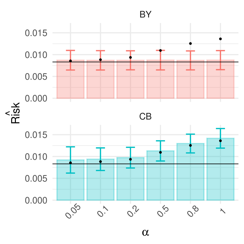
(a) Ridge regression, fixed $\lambda$

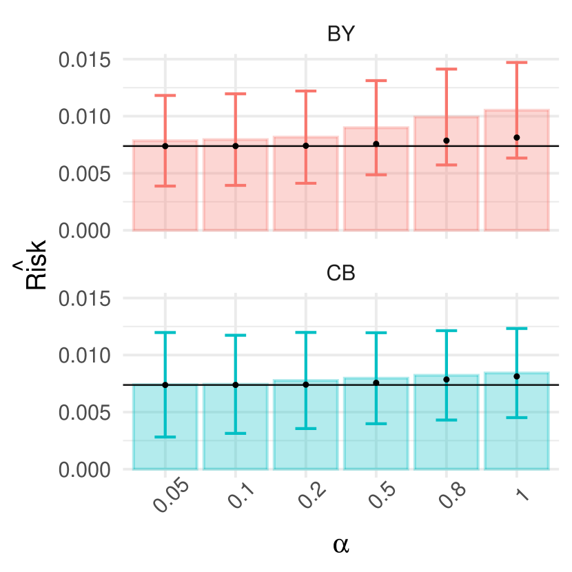
(b) Lasso regression, fixed $\lambda$

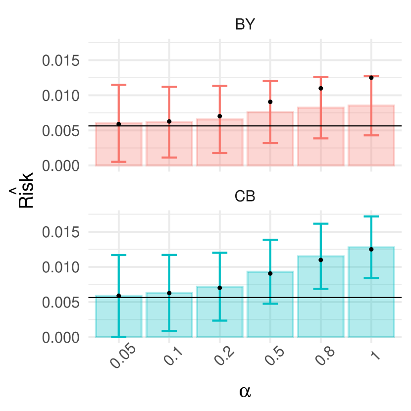
(c) Forward stepwise, fixed $k$

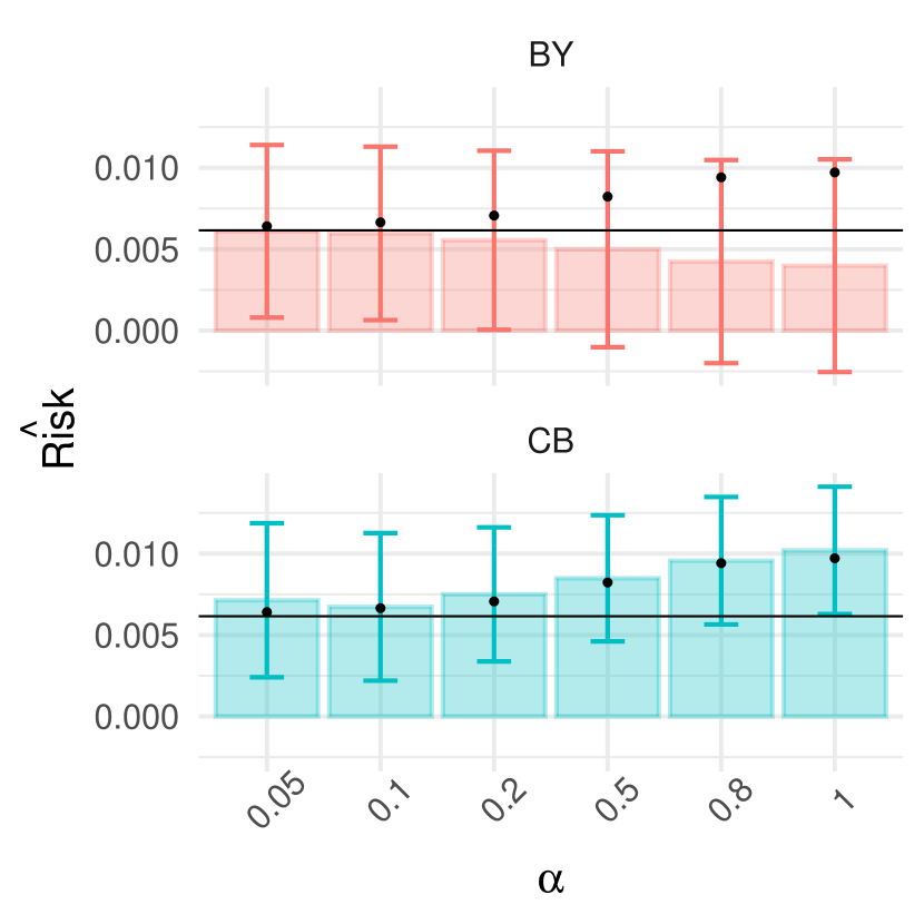
(d) Lasso regression, CV-tuned $\lambda$

Figure 1: Comparison of risk estimators for different functions $g$, when $s=5$ and $\mathrm{SNR}=0.4$.

Figure 1 shows the results for when the underlying linear model has sparsity $s=5$, and $\mathrm{SNR}=0.4$. The figure displays the average risk estimate from each method, CB and BY, as well as standard errors of these risk estimates. Each panel (a)–(d) corresponds to one of the four functions $g$ described above. In each panel, the black horizontal line represents $\mathrm{Risk}(g)$, and the black dots represent $\mathrm{Risk}_{\alpha}(g)$ (which are themselves estimated via Monte Carlo). We can see that, for each function $g$, the CB method is unbiased for $\mathrm{Risk}_{\alpha}(g)$, as expected. Meanwhile, we see that the bias of the BY method varies quite a lot with $g$, having zero, positive, or negative bias, depending on the situation. In panel (a), where $g$ is a linear smoother (ridge), the average BY estimate matches $\mathrm{Risk}(g)$, regardless of $\alpha$, as expected. In (b), where $g$ is nonlinear but is still weakly differentiable (lasso), it overestimates $\mathrm{Risk}_{\alpha}(g)$, and thus also $\mathrm{Risk}(g)$, dramatically so at the larger values of $\alpha$. In panel (c), where $g$ is both nonlinear and nonsmooth (forward stepwise), it underestimates $\mathrm{Risk}_{\alpha}(g)$, and yet it overestimates $\mathrm{Risk}(g)$, for larger $\alpha$; and in (d), where $g$ is again nonlinear and nonsmooth (lasso tuned by cross-validation), it underestimates both $\mathrm{Risk}_{\alpha}(g)$ and $\mathrm{Risk}(g)$ for larger $\alpha$. In summary, there is no single consistent behavior for the bias of $\mathrm{BY}_{\alpha}(g)$ across all scenarios.

While for small $\alpha$, the average BY estimate appears to be empirically close to $\mathrm{Risk}(g)$ in all situations (as does the average CB estimate), we reiterate that there is no guarantee this will be true in general for nonsmooth $g$ (as in panels (c) and (d)). However, the average CB estimate will always be close to $\mathrm{Risk}_{\alpha}(g)$, which will be in turn close to $\mathrm{Risk}(g)$ for small $\alpha$, no matter the smoothness of $g$ (Propositions 2 and 3).

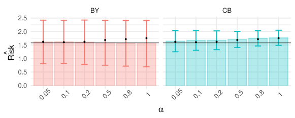
Figure 2: Comparison of risk estimators when $g$ is the lasso tuned by cross-validation, $s=200$, and $\mathrm{SNR}=2$.

In the previous figure, the variability of the BY and CB estimates (reflected in the standard error bars) appears roughly similar throughout. In Figure 2, we demonstrate that this need not be the case in general. By increasing the true sparsity level to $s=200$ (the true linear model is dense) and the signal-to-noise ratio to $\mathrm{SNR}=2$, we see that the BY estimates appear much more volatile than those from CB, when we take $g$ to be the lasso tuned by cross-validation. This holds across all values of $\alpha$. In Appendix F, we show that the larger variance of BY in this setting is due to its irreducible variance, and in particular, just one part of its irreducible variance: comparing (39) and (43), we see that the only difference between the two is the first term (inside the variance). In CB, this is the conditional expectation of the noise-added training error, and in BY, it is the training error itself. When $g$ is unstable, as in the current setting (the use of cross-validation for tuning induces instability into the ultimate prediction function), the latter can be much more variable.

5.2 Degrees of freedom

Recalling Efron’s covariance decomposition (8), and the definition of degrees of freedom (7), it is clear that estimating $\mathrm{Risk}(g)$ and estimating $\mathrm{df}(g)$ are equivalent problems, in the normal means setting. Thus, parallel to the perspective and development used in this paper, where the CB method (19) is crafted as an unbiased estimator of $\mathrm{Risk}_{\alpha}(g)$, the risk of $g$ at the inflated noise level of $(1+\alpha)\sigma^{2}$, we can equivalently view:

$$\widehat{\mathrm{df}}_{\alpha}(g)=\frac{\mathrm{CB}_{\alpha}(g)-\frac{1}{B}\sum_{b=1}^{B}\|Y^{*b}-g(Y^{*b})\|_{2}^{2}+n\sigma^{2}(1+\alpha)}{2\sigma^{2}(1+\alpha)}$$ (44)

as an unbiased estimator of $\mathrm{df}_{\alpha}(g)$, the degrees of freedom of $g$ at the inflated noise level $(1+\alpha)\sigma^{2}$. For the BY method, meanwhile, one can proceed similarly in moving from (12) to an estimator of degrees of freedom (by subtracting off training error and rescaling); however, there is an alternative, more direct estimator that stems from this method, which was the original proposal of Ye (1998), namely:

$$\widetilde{\mathrm{df}}_{\alpha}(g)=\frac{1}{\sigma^{2}\alpha}\sum_{i=1}^{B}\widehat{\mathrm{Cov}}_{i}^{*},$$ (45)

where $\widehat{\mathrm{Cov}}_{i}^{*}$, $i=1,\ldots,n$, are as in (10). While $\widehat{\mathrm{df}}_{\alpha}(g)$ estimates $\mathrm{df}_{\alpha}(g)$ (unbiasedly), it seems that $\widetilde{\mathrm{df}}_{\alpha}(g)$ is designed to directly estimate $\mathrm{df}(g)$ (though not unbiasedly).

In Figure 3, we evaluate the performance of these two degrees of freedom estimators (44), (45) using the same simulation framework as that described in the last subsection, with $s=5$ and $\mathrm{SNR}=2$. We consider two functions $g$: lasso and forward stepwise, and for each, we vary their tuning parameters over their effective ranges. Lastly, we fix $\alpha=0.1$. The figure displays the estimated degrees of freedom from CB (44) or BY (45), against the support size of the underlying fitted sparse regression model (for the lasso, we take this to be the average support size for the given value of $\lambda$ over all 100 repetitions): the bands represent the degrees of freedom estimate plus and minus one standard error, over the 100 repetitions. The true degrees of freedom (itself estimated via Monte Carlo) is shown as a dashed line; note, this is the degrees of freedom $\mathrm{df}(g)$ at the original noise level, not the noise-elevated degrees of freedom $\mathrm{df}_{\alpha}(g)$. We see that both methods provide reasonably accurate estimates of degrees of freedom throughout, albeit slightly biased upwards at various points along the path (support sizes), due to the use of $\alpha=0.1$. Reducing $\alpha$ would reduce the bias, but also increase the variability in the estimates. We also see that the estimates of degrees of freedom from the CB method are just a bit more variable across the lasso path, and most noticeably so at the smallest support sizes.

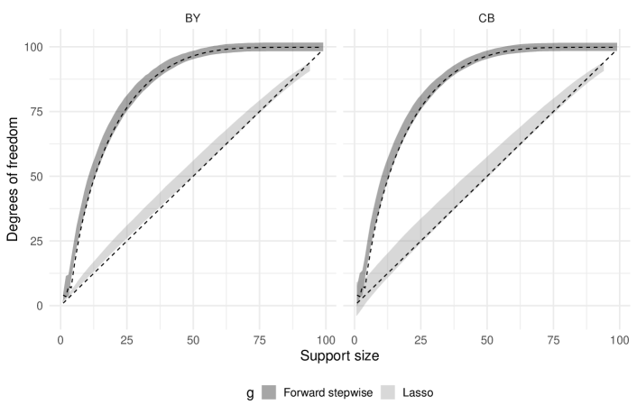
Figure 3: Comparison of degrees of freedom estimators applied to the full forward stepwise and lasso paths, when $s=5$, $\mathrm{SNR}=2$, and $\alpha=0.1$.

5.3 Image denoising

As a last example, we consider using the CB method for tuning parameter selection in image denoising. In image denoising, and signal processing more broadly, SURE has become a central method for risk estimation and parameter tuning (see Section 1.7 for references). We focus on the 2-dimensional fused lasso (Tibshirani et al., 2005; Hoefling, 2010) as an image denoising estimator, as it is weakly differentiable and its divergence can be computed in analytic form (Tibshirani and Taylor, 2011, 2012). This allows us to draw a comparison to SURE, which takes the simple form:

$$\mathrm{SURE}(g)=\|Y-g(Y)\|_{2}^{2}+2\sigma^{2}\big{(}\text{\# of fused groups in $g(Y)$}\big{)}-n\sigma^{2}.$$

To compare the CB estimator (19) and SURE (above) empirically, we use the standard “Lena” image from the image processing literature (leftmost panel of Figure 5), and generate data $Y$ by adding i.i.d. normal noise to each pixel (second from the left in Figure 5). Figure 5 compares SURE (dashed line) and the CB estimator (solid lines) across several values of $\alpha$, each as functions of the underlying tuning parameter $\lambda$ in the 2d fused lasso lasso optimization problem. The true risk is also plotted (dotted line). The primary conclusion is that, for all values of $\alpha$ (even the largest one $\alpha=0.5$), the minimizers of the $\mathrm{CB}_{\alpha}(g)$ curve are all close to that of $\mathrm{SURE}(g)$, which means that the subsequent CB-tuned and SURE-tuned estimates are themselves all quite similar (second to right and rightmost panels of Figure 5). This speaks—informally—to model selection being “easier” than risk estimation in this context, since we can get away with larger values of $\alpha$ and still make the relevant risk comparisons needed in order to accurately select a model (indexed by a tuning parameter).

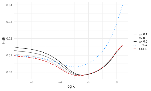
Figure 4: Comparison of the CB estimator and SURE for image denoising.

Figure 5: Original “Lena” image (leftmost), and a noisy version (second from left) used for image denoising. The CB-tuned (second from right, using $\alpha=0.1$) and SURE-tuned (righmost) estimates look very similar.

6 Discussion

In this work, we proposed and studied a coupled bootstrap (CB) method for risk estimation in the standard normal means problem. Our estimator is on one hand similar to bootstrap-based proposals for risk estimation (via a covariance decomposition) in this setting from Breiman (1992); Ye (1998); Efron (2004). On the other hand, it is different in a key way: for any value of the auxiliary (bootstrap) noise parameter $\alpha>0$, the CB estimator is unbiased for $\mathrm{Risk}_{\alpha}(g)$, the risk of the function $g$ in question, when the noise level in the normal means problem is inflated from $\sigma^{2}$ to $(1+\alpha)\sigma^{2}$. We proved that for a weakly differentiable function $g$, the CB estimator (with infinite bootstrap iterations) reduces to SURE as $\alpha\to 0$, just like the Breiman-Ye estimator does in this noiseless limit. However, for nonsmooth $g$, and arbitrary non-infinitesimal $\alpha$, the CB estimator still tracks an intuitively reasonable target: $\mathrm{Risk}_{\alpha}(g)$. Indeed, the unbiasedness of the CB estimator for $\mathrm{Risk}_{\alpha}(g)$ makes no assumptions on $g$ whatsoever. As such, it can be applied to arbitrarily complex functions $g$, including those that use some sort of internal tuning parameter selection mechanism.

Of course, one of the most important practical problems not addressed in the current paper is estimation of the error variance $\sigma^{2}$. In practice, the simplest strategies here tend to be among the most commonly-used, and among the most effective: we could simply estimate $\sigma^{2}$ by using the sample variance of training residuals $Y_{i}-g_{i}(Y)$, $i=1,\ldots,n$ (possibly with a degrees of freedom correction, which can be important for complex models $g$). A study of the impact of estimating $\sigma^{2}$ on risk estimation and model selection is a topic for future work. (For model selection, we may not actually need to estimate $\sigma^{2}$ up to the same degree of accuracy as we would in risk estimation; recall, we have already seen that relative large values of the auxiliary noise level $\alpha>0$ can still result in good model selection performance, in Figure 5.)

Two more extensions of the CB framework that may be of interest for future work are described below.

6.1 Structured errors

Consider, instead of (1), data drawn according to:

$$Y\sim N(\theta,\Sigma),$$ (46)

for a positive definite covariance matrix $\Sigma\in\mathbb{R}^{n\times n}$. In such a structured error setting, it may be of interest to measure loss according to a generalized quadratic norm, thus we introduce the notation $\|x\|_{A}^{2}=x^{\mathsf{T}}A^{-1}x$ for a vector $x$ and positive semidefinite matrix $A$. For example, we may choose to measure loss according to $\|\theta-g(Y)\|_{\Sigma}^{2}$, since the curvature in this loss takes $\Sigma$ into account, just like the negative log-likelihood in the model (46).

We extend the CB estimator so that it applies to an arbitrary positive semidefinite matrix $A$ defining the risk, and an arbitrary positive semidefinite matrix $\Sigma$ in (46). The next result is a straightforward extension of Proposition 1.

Proposition 6.

Let $U,V,W\in\mathbb{R}^{n}$ be independent random vectors. Then for any $g$, and positive semidefinite matrix $A\in\mathbb{R}^{n\times n}$,

$$\mathbb{E}\|V-g(U)\|_{A}^{2}-\mathbb{E}\|W-g(U)\|_{A}^{2}=\mathbb{E}\|V\|_{A}^{2}-\mathbb{E}\|W\|_{A}^{2}+2\langle A^{-1}\mathbb{E}[g(U)],\mathbb{E}[W]-\mathbb{E}[V]\rangle.$$ (47)

In particular, if $\mathbb{E}[V]=\mathbb{E}[W]$ and $U,V$ are i.i.d., then

$$\mathbb{E}\|V-g(U)\|_{A}^{2}=\mathbb{E}\|W-g(U)\|_{A}^{2}+\mathbb{E}\|U\|_{A}^{2}-\mathbb{E}\|W\|_{A}^{2}.$$ (48)

And in turn, the next result is a straightforward extension of Corollary 1.

Corollary 2.

Let $Y\sim N(\theta,\Sigma)$. Given any function $g$, a positive semidefinite matrix $A\in\mathbb{R}^{n\times n}$ that will be used to measure risk, and an auxiliary noise level $\alpha>0$, consider defining a CB estimator according to:

$$\begin{gathered}\omega^{b}\sim N(0,\Sigma),\quad b=1,\ldots,B\;\,\text{(independently)},\\ Y^{*b}=Y+\sqrt{\alpha}\omega^{b},\quad,Y^{\dagger{b}}=Y-\omega^{b}/\sqrt{\alpha},\quad b=1,\ldots,B,\end{gathered}$$ (49)

and:

$$\mathrm{CB}_{A,\alpha}(g)=\frac{1}{B}\sum_{b=1}^{B}\Big{(}\|Y^{\dagger{b}}-g(Y^{*b})\|^{2}_{A}-\|\omega^{b}\|_{A}^{2}/\alpha\Big{)}-\mathrm{tr}(A^{-1}\Sigma).$$ (50)

Then this is unbiased for risk at the noise-elevated level $(1+\alpha)\Sigma$ measured with respect to $A$, i.e.,

$$\mathbb{E}[\mathrm{CB}_{A,\alpha}(g)]=\mathrm{Risk}_{A,\alpha}(g)=\mathbb{E}\|\theta-g(Y_{\alpha})\|_{A}^{2},\quad\text{where $Y_{\alpha}\sim N(\theta,(1+\alpha)\Sigma)$}.$$

Of course, the main challenge in using the extended estimator $\mathrm{CB}_{A,\alpha}(g)$ defined in the above corollary is that it requires knowledge of the full error covariance matrix $\Sigma$. However, in some settings, e.g., time series problems, it may be reasonable to assume that $\Sigma$ or its inverse is highly structured and therefore estimable. It may be interesting to rigorously study how risk estimation is affected by upstream estimation of $\Sigma$ in this and related problem settings.

6.2 Bregman divergence

Lastly, we present a further extension of the simple and yet key results in Proposition 6 underpinning the construction of the CB estimator, to the case in which a Bregman divergence is used to measure error:

$$\mathrm{Err}_{\phi}(g)=\mathbb{E}[D_{\phi}(\tilde{Y},g(Y))],\quad\text{where $\tilde{Y}$ is an i.i.d.\ copy of $Y$}.$$ (51)

Here $D_{\phi}$ is the Bregman divergence with respect to a strictly convex and differentiable function $\phi:\mathbb{R}^{n}\to\mathbb{R}$, which recall is defined by:

$$D_{\phi}(a,b)=\phi(a)-\phi(b)-\langle\nabla\phi(b),a-b\rangle.$$

When $\phi(x)=\|x\|_{2}^{2}$, it is easy to check that

$$D_{\|\cdot\|_{2}^{2}}(a,b)=\|a\|_{2}^{2}-\|b\|_{2}^{2}-2\langle b,a-b\rangle=\|a-b\|_{2}^{2},$$

and hence (51) reduces to prediction error as measured by squared loss in (4). In fact, properties (47), (48) are entirely driven by the above “Bregman representation” of squared error. This immediately leads to the following extension.

Proposition 7.

Let $U,V,W\in\mathbb{R}^{n}$ be independent random vectors. For any $g$, and Bregman divergence $D_{\phi}$,

$$\mathbb{E}[D_{\phi}(V,g(U))]-\mathbb{E}[D_{\phi}(W,g(U))]=\mathbb{E}[\phi(V)]-\mathbb{E}[\phi(W)]+\langle\mathbb{E}[\nabla\phi(U)],\mathbb{E}[W]-\mathbb{E}[V]\rangle.$$ (52)

In particular, if $\mathbb{E}[V]=\mathbb{E}[W]$ and $U,V$ are i.i.d., then

$$\mathbb{E}[D_{\phi}(V,g(U))]=\mathbb{E}[D_{\phi}(W,g(U))]+\mathbb{E}[\phi(U)]-\mathbb{E}[\phi(W)].$$ (53)

Proposition 7 is, in principle, a powerful tool: it provides “one half” of a recipe to move the CB estimator beyond the Gaussian setting, to a setting in which data follows (say) an exponential family distribution and loss is measured by the out-of-sample deviance. This is because for every exponential family distribution, there is a natural function $\phi$ (defined in terms of the log-partition function of the distribution) that makes (51) the deviance.

The “other half” of the recipe needed to arrive at a CB estimator is a mechanism for generating relevant bootstrap draws, as in (49) in the previous subsection. Specifically, for a given problem setting with data $Y$ (exponential family distributed or otherwise) we must be able to design a pair of bootstrap draws $(Y^{*b},Y^{\dagger{b}})$ that adhere to three criteria:

1. $Y^{*b},Y^{\dagger{b}}$ are independent of each other;

2. $\mathbb{E}[Y^{*b}]=\mathbb{E}[Y^{\dagger{b}}]$; and

3. $\mathbb{E}[D_{\phi}(\tilde{Y}^{*b},g(Y^{*b}))]$ is an “interesting” pseudo-target to estimate, where $\tilde{Y}^{*b}$ is an i.i.d. copy of $Y^{*b}$.

Criteria 1 and 2 are straightforward enough to understand, and they should be possible to fulfill in certain exponential family models with various noise augmentation tricks. However, criterion 3 deserves a bit more explanation. With $U=Y^{*b}$, $V=\tilde{Y}^{*b}$, and $W=Y^{\dagger{b}}$, assumed to fulfill criteria 1 and 2, note that (53) says $D_{\phi}(Y^{\dagger{b}},g(Y^{*b}))$ is unbiased for $\mathbb{E}[D_{\phi}(\tilde{Y}^{*b},g(Y^{*b}))]$. That is, we originally wanted to estimate the quantity in (51), and have now pivoted to estimating $\mathbb{E}[D_{\phi}(\tilde{Y}^{*b},g(Y^{*b}))]$ instead.

In the Gaussian setting studied throughout this paper, this meant estimating risk based on data from a Gaussian distribution with the same mean but an inflated noise level. In a more general setting, the noise augmentation strategy used to generate $Y^{*b}$ may in fact bring us outside of the distributional family assumed for the original data $Y$, and it may even alter non-nuisance parameters of the distribution; this would still altogether be fine, as long as $\mathbb{E}[D_{\phi}(\tilde{Y}^{*b},g(Y^{*b}))]$ it still an “interesting” target (i.e., for error assessment or model selection), as per criterion 3.

Acknowledgements

RJT is grateful to Xiaoying Tian for providing the inspiration to work on this project in the first place, and Saharon Rosset for early insightful conversations. NLO was supported by an Amazon Fellowship.

Appendix A More details on Breiman’s and Ye’s estimators

Instead of defining $\widehat{\mathrm{Cov}}_{i}^{*}$, $i=1,\ldots,n$ as in (10), Breiman uses

$$\widehat{\mathrm{Cov}}_{i}^{*}=\frac{1}{B-1}\sum_{b=1}^{B}(Y_{i}^{*b}-Y_{i})g_{i}(Y^{*b}),\quad i=1,\ldots,n,$$

which are just inner products between the noise increments $\{Y_{i}^{*b}-Y_{i}\}_{b=1}^{B}$ and fitted values $\{g_{i}(Y^{*b})\}_{b=1}^{B}$, instead of an empirical covariances.

Furthermore, instead of dividing the whole sum by $\alpha$, Ye divides each summand $\widehat{\mathrm{Cov}}_{i}^{*}$ in (12) by

$$(s^{*}_{i})^{2}=\frac{1}{B-1}\sum_{b=1}^{B}(Y_{i}^{*b}-\bar{Y}_{i}^{*})^{2},$$

the bootstrap estimate of the variance of $Y_{i}$, rather than dividing the entire sum by $\alpha$. In fact, Ye actually formulates his estimator in terms of the slopes from linearly regressing the fitted values $\{g_{i}(Y^{*b})\}_{b=1}^{B}$ onto the noise increments $\{Y_{i}^{*b}-Y_{i}\}_{b=1}^{B}$, but it is equivalent to the form described here.

Appendix B Proof of Proposition 2

The proposition follows from an application of the next lemma, as we can take $f(y)=\|\theta-g(y)\|_{2}^{2}$, and then the moment conditions on $f$ will be implied by those on $\|g\|_{2}^{2}$, via the simple bound $f(y)\leq 2\|\theta\|_{2}^{2}+2\|g(y)\|_{2}^{2}$.

Lemma 1.

For $\alpha\geq 0$, denote $Y_{\alpha}\sim N(\theta,(1+\alpha)\sigma^{2}I_{n})$. Let $f:\mathbb{R}^{n}\to\mathbb{R}$ be a function such that, for some $\beta>0$ and integer $k\geq 0$,

$$\mathbb{E}\big{[}f(Y_{\beta})\|Y_{\beta}-\theta\|_{2}^{2m}\big{]}<\infty,\quad m=0,\ldots,k.$$

Then, the map $\alpha\mapsto\mathbb{E}[f(Y_{\alpha})]$ has $k$ continuous derivatives on $[0,\beta)$.

Proof.

First, we prove that this map is continuous. Fix $\alpha\in[0,\beta)$. Observe that

$$\lim_{t\to\alpha}\mathbb{E}[f(Y_{t})] =\lim_{t\to\alpha}\int\frac{f(y)}{(2\pi(1+t)\sigma^{2})^{n/2}}\exp\bigg{\{}\frac{-\|y-\theta\|^{2}}{2(1+t)\sigma^{2}}\bigg{\}}\,dy$$

$$=\int\lim_{t\to\alpha}\frac{f(y)}{(2\pi(1+t)\sigma^{2})^{n/2}}\exp\bigg{\{}\frac{-\|y-\theta\|^{2}}{2(1+t)\sigma^{2}}\bigg{\}}\,dy$$

$$=\mathbb{E}[f(Y_{\alpha})],$$

where in the second line we used Lebesgue’s dominated convergence theorem (DCT), applicable because the integrand is bounded by

$$\frac{f(y)}{(2\pi\sigma^{2})^{n/2}}\exp\bigg{\{}\frac{-\|y-\theta\|^{2}}{2(1+\alpha)\sigma^{2}}\bigg{\}},$$

which is integrable by assumption. Now for the first derivative, note that

$$\frac{\partial}{\partial\alpha}\mathbb{E}[f(Y_{\alpha})]=-\frac{n}{2(1+\alpha)}\mathbb{E}[f(Y_{\alpha})]+\frac{1}{2\sigma^{2}(1+\alpha)^{2}}\mathbb{E}[f(Y_{\alpha})\|Y_{\alpha}-\theta\|_{2}^{2}],$$

where we used the Leibniz integral rule, applicable because the integrands (when we write these expectations as integrals) are bounded by

$$\frac{f(y)}{(2\pi\sigma^{2})^{n/2}}\|y-\theta\|_{2}^{2m}\exp\bigg{\{}\frac{-\|y-\theta\|^{2}}{2(1+\alpha)\sigma^{2}}\bigg{\}},$$

for $m=0,1$, again integrable by assumption. Another application of DCT proves the derivative in the second to last display is continuous on $[0,\beta)$. For a general number of derivatives $k$, the argument is similar, and the integrability of the dominating functions in the above display, for $m=0,\ldots,k$, ensures that we can apply the Leibniz rule and DCT to argue continuity of the $k$th derivative on $[0,\beta)$. ∎

Appendix C Proof of Theorem 2

C.1 Proof of theorem

Observe that, writing $\mathbb{E}_{\omega}$ for the conditional expectation operator on $Y=y$ (i.e., the operator that integrates over $\omega$),

$$\mathrm{CB}_{\alpha}^{\infty}(g) =\mathbb{E}_{\omega}\big{[}\|y-\omega/\sqrt{\alpha}-g(y+\sqrt{\alpha}\omega)\|_{2}^{2}-\|\omega\|_{2}^{2}/\alpha\big{]}-n\sigma^{2}$$

$$=\underbrace{\vphantom{\frac{2}{\sqrt{\alpha}}}\mathbb{E}_{\omega}\|y-g(y+\sqrt{\alpha}\omega)\|_{2}^{2}}_{a}\,-\,\underbrace{\frac{2}{\sqrt{\alpha}}\mathbb{E}_{\omega}\langle\omega,g(y+\sqrt{\alpha}\omega)\rangle}_{b}-n\sigma^{2}.$$

It is not hard to show that for almost every $y\in\mathbb{R}^{n}$, it holds that $a\to\|y-g(y)\|_{2}^{2}$ as $\alpha\to 0$, by Lemma 3. It remains to study term $b$.

Denote by $\phi_{\mu,\sigma^{2}}$ the density of a Gaussian with mean $\mu$ and variance $\sigma^{2}$. Then,

$$b =\frac{2}{\sqrt{\alpha}}\sum_{i=1}^{n}\mathbb{E}_{\omega_{-i}}\mathbb{E}_{\omega_{i}}[\omega_{i}g_{i}(y+\sqrt{\alpha}\omega)]$$

$$=\frac{2}{\sqrt{\alpha}}\sum_{i=1}^{n}\mathbb{E}_{\omega_{-i}}\int\omega_{i}g_{i}(y+\sqrt{\alpha}\omega)\phi_{0,\sigma^{2}}(\omega_{i})\,d\omega_{i}$$

$$=-\frac{2\sigma^{2}}{\sqrt{\alpha}}\sum_{i=1}^{n}\mathbb{E}_{\omega_{-i}}\int g_{i}(y+\sqrt{\alpha}\omega)\phi^{\prime}_{0,\sigma^{2}}(\omega_{i})\,d\omega_{i}$$

$$=-2\sigma^{2}\sum_{i=1}^{n}\mathbb{E}_{u_{-i}}\int g_{i}(u)\phi^{\prime}_{0,\alpha\sigma^{2}}(u_{i}-y_{i})\,d\omega_{i}$$

$$=2\sigma^{2}\sum_{i=1}^{n}\mathbb{E}_{u_{-i}}\int\nabla_{i}g_{i}(u)\phi_{0,\alpha\sigma^{2}}(u_{i}-y_{i})\,d\omega_{i}$$

$$=2\sigma^{2}\sum_{i=1}^{n}\int\nabla_{i}g_{i}(u)\phi_{0,\alpha\sigma^{2}}(u-y)\,du.$$

The second to last line holds by Lemma 2. Now, by Lemma 3, for almost every $y\in\mathbb{R}^{n}$,

$$\lim_{\alpha\to 0}2\sigma^{2}\sum_{i=1}^{n}\int\nabla_{i}g_{i}(u)\phi_{0,\alpha\sigma^{2}}(u-y)\,du=2\sigma^{2}\sum_{i=1}^{n}\nabla_{i}g_{i}(y),$$

which completes the proof.

C.2 Supporting lemmas

Here we state and prove supporting lemmas for the proof of Theorem 2. The first lemma shows that for a weakly differentiable function, the integration by parts property in (27) still holds when we take the test function to be a normal density (which is continuously differentiable by not compactly supported).

Lemma 2.

If $f:\mathbb{R}\to\mathbb{R}$ is weakly differentiable, with $(f\phi_{\mu,\sigma^{2}})\in L^{1}(\mathbb{R})$ and $(f^{\prime}\phi_{\mu,\sigma^{2}})\in L^{1}(\mathbb{R})$, then

$$\int f(x)\phi^{\prime}_{\mu,\sigma^{2}}(x)\,dx=-\int f^{\prime}(x)\phi_{\mu,\sigma^{2}}(x)\,dx.$$

Proof.

Let $\psi_{n}:\mathbb{R}\to[0,1]$, $n=1,2,3,\ldots$ be a sequence of continuously differentiable functions such that for each $z\in\mathbb{R}$,

$$\lim_{n\to\infty}\psi_{n}(z)=1,\quad\lim_{n\to\infty}\psi_{n}^{\prime}(z)=0,\quad\text{and}\quad|\psi_{n}^{\prime}(z)|\leq C\;\,\text{for $n=1,2,3,\ldots$ and a constant $C<\infty$}.$$

One example of such a sequence is

$$\psi_{n}(z)=1_{(-n,n)}(z)+\exp\bigg{(}-\frac{1}{1-(z-n\mathrm{sign}(z))}\bigg{)}1_{[-n-1,-n]\cup[n,n+1]}(z),\quad n=1,2,3,\ldots.$$

Now let $\xi_{n}(z)=\psi_{n}(z)\phi_{\mu,\sigma^{2}}(z)$. Note that

$$\lim_{n\to\infty}\xi_{n}(z) =\phi_{\mu,\sigma^{2}}(z)\lim_{n\to\infty}\psi_{n}(z)=\phi_{\mu,\sigma^{2}}(z),$$

$$\lim_{n\to\infty}\xi^{\prime}_{n}(z) =\lim_{n\to\infty}\psi^{\prime}_{n}(z)\phi_{\mu,\sigma^{2}}(z)+\phi_{\mu,\sigma^{2}}^{\prime}(z)\lim_{n\to\infty}\psi_{n}(z)=\phi_{\mu,\sigma^{2}}^{\prime}(z).$$

Turning to the result we want to prove,

$$\int f(z)\phi_{\mu,\sigma^{2}}^{\prime}(z)\,dz =\int f(z)\lim_{n\to\infty}\xi^{\prime}_{n}(z)\,dz$$

$$=\lim_{n\to\infty}\int f(z)\xi^{\prime}_{n}(z)\,dz$$

$$=-\lim_{n\to\infty}\int f^{\prime}(z)\xi_{n}(z)\,dz$$

$$=-\int f^{\prime}(z)\lim_{n\to\infty}\xi_{n}(z)\,dz$$

$$=-\int f^{\prime}(z)\phi_{\mu,\sigma^{2}}(z)\,dz.$$

The second and fourth lines here can be verified using Lebesgue’s dominated convergence theorem (DCT), and the third uses (27), applicable because each $\xi_{n}$ is compactly supported. This completes the proof. ∎

The next lemma essentially shows that the notion of a Lebesgue point can be extended to the Gaussian kernel (beyond the uniform kernel, as it is traditionally defined).

Lemma 3 (Adapted from Theorem 1.25 of Stein and Weiss 1971).

Let $\phi:\mathbb{R}^{n}\to\mathbb{R}$ be the Gaussian density with mean zero and identity covariance, and denote $\phi_{\alpha}=\alpha^{-n}\phi(x/\alpha)$. Let $f:\mathbb{R}^{n}\to\mathbb{R}$ be a function such that $(f\phi_{\beta})\in L^{1}(\mathbb{R}^{n})$ for some $\beta>0$. Then, $\lim_{\alpha\to 0}(f*\phi_{\alpha})(x)=f(x)$ for almost every $x\in\mathbb{R}^{n}$.

Proof.

Let $x\in\mathbb{R}^{n}$ be a Lebesgue point of $f$. We will prove that the desired result holds for $x$, which will imply that it holds almost everywhere (because any function in $L^{1}_{\mathrm{loc}}(\mathbb{R}^{n})$ has the property that almost every point is a Lebesgue point; see, e.g., Theorem 1.32 of Evans and Gariepy (2015)).

Fix $\epsilon>0$. By the definition of a Lebesgue point, there exists $\rho>0$ such that

$$\delta^{-n}\int_{\|t\|_{2}\leq\delta}|f(x-t)-f(x)|\,dt\leq C\epsilon,$$ (54)

for all $\delta\in(0,\rho]$ and a constant $C>0$ to be specified later. In what follows, we will show that there exists $\beta>0$ such that $|(f*\phi_{\alpha})(x)-f(x)|\leq\epsilon$ for all $\alpha\in(0,\beta]$. To do so, we decompose

$$|(f*\phi_{\alpha})(x)-f(x)|\leq\underbrace{\bigg{|}\int_{\|t\|_{2}\leq\delta}(f(x-t)-f(x))\phi_{\alpha}(t)\,dt\bigg{|}}_{I_{1}}\,+\,\underbrace{\bigg{|}\int_{\|t\|_{2}>\delta}(f(x-t)-f(x))\phi_{\alpha}(t)\,dt\bigg{|}}_{I_{2}}.$$ (55)

We study each term above separately.

Term $I_{1}$.

Let $g(r)=\int_{\|t\|_{2}=1}|f(x-rt)-f(x)|\,dt$ and $G(r)=\int_{0}^{r}s^{n-1}g(s)\,ds$. Note that (54) translates into the statement

$$G(r)\leq C\epsilon r^{n},$$ (56)

for all $r\in(0,\rho]$.

For notational convenience, we write $\varphi(r)=\phi(u)$ whenever $\|u\|_{2}=r$, where $\varphi$ is the univariate standard normal density. Observe that for any $\delta\leq\rho$,

$$I_{1} \leq\int_{\|t\|_{2}\leq\delta}|f(x-t)-f(x)|\alpha^{-n}\phi(t/\alpha)\,dt$$

$$=\int_{0}^{\delta}r^{n-1}g(r)\alpha^{-n}\varphi(r/\alpha)\,dr$$

$$=G(r)\alpha^{-n}\varphi(r/\alpha)\big{|}_{0}^{\delta}-\alpha^{-n}\int_{0}^{\delta}G(r)\,d(\varphi(r/\alpha))$$

$$\leq C\epsilon(\delta/\alpha)^{n}\varphi(\delta/\alpha)-\alpha^{-n}\int_{0}^{\delta}G(r)\,d(\varphi(r/\alpha))$$

$$=C\epsilon(\delta/\alpha)^{n}\varphi(\delta/\alpha)-\alpha^{-n}\int_{0}^{\delta/\alpha}G(\alpha s)\,d(\varphi(s))$$

$$\leq C\epsilon(\delta/\alpha)^{n}\varphi(\delta/\alpha)+C\epsilon\int_{0}^{\delta/\alpha}s^{n}\,|d(\varphi(s))|$$

$$\leq C\epsilon(c_{n}+m_{n+1}).$$

In the fourth and sixth lines, we used (56). In the last line, we used the fact the map $z\mapsto z^{n}\varphi(z)$ attains a maximum of $c_{n}=\sqrt{n}^{n}\phi(\sqrt{n})$ at $z=\sqrt{n}$, as well as the bound $\int_{0}^{\delta/\alpha}s^{n}\,|d(\varphi(s))|\leq\int_{0}^{\infty}s^{n+1}\varphi(s)\,ds\leq m_{n+1}$, where $m_{n+1}$ uncentered, absolute moment of order $n+1$ of the standard normal distribution. By choosing $C\leq 1/(2(c_{n}+m_{n+1}))$, we see that $I_{1}\leq\epsilon/2$ for any $\delta\leq\rho$, and any $\alpha>0$.

Term $I_{2}$.

Consider

$$I_{2}=\underbrace{\int_{\|t\|_{2}\geq\delta}|f(x-t)|\phi_{\alpha}(t)\,dt}_{I_{21}}\,+\,\underbrace{|f(x)|\int_{\|t\|_{2}\geq\delta}\phi_{\alpha}(t)\,dt}_{I_{22}}.$$

Clearly

$$\lim_{\alpha\to 0}I_{22}=|f(x)|\lim_{\alpha\to 0}\int_{\|u\|_{2}\geq\delta/\alpha}\phi(u)\,du=0,$$

so there exists $\beta_{1}>0$ such that for $\alpha\leq\beta_{1}$, we have $I_{22}\leq\epsilon/4$. As for $I_{21}$, we have

$$\lim_{\alpha\to 0}I_{21}=\lim_{\alpha\to 0}\int_{\|t\|_{2}\geq\delta}|f(x-t)|\phi_{\alpha}(t)\,dt=\int_{\|t\|_{2}\geq\delta}\lim_{\alpha\to 0}|f(x-t)|\phi_{\alpha}(t)\,dt=0,$$

where the interchange between integration and the limit as $\alpha\to 0$ can be shown using DCT. Thus there is $\beta_{2}>0$ such that for $\alpha\leq\beta_{2}$, we have $I_{21}<\epsilon/4$.

Completing the proof.

Putting the above parts together, we get that $I_{1}+I_{2}\leq\epsilon/2+\epsilon/4+\epsilon/4=\epsilon$, for all $\delta\leq\rho$ and $\alpha\leq\beta=\min\{\beta_{1},\beta_{2}\}$. Recalling (55), this gives the desired result and completes the proof. ∎

Appendix D Noiseless limit for hard-thresholding

The limit in question is that of

$$\frac{2}{\sqrt{\alpha}}\sum_{i=1}^{n}\mathbb{E}\big{[}\omega_{i}(y_{i}+\sqrt{\alpha}\omega_{i})\cdot 1\{|y_{i}+\sqrt{\alpha}\omega_{i}|>t\}\big{]}$$

as $\alpha\to 0$. Inspecting term $i$,

$$\mathbb{E}\big{[}\omega_{i}(y_{i}+\sqrt{\alpha}\omega_{i})\cdot 1\{|y_{i}+\sqrt{\alpha}\omega_{i}|>t\}\big{]} =\frac{y}{\sqrt{\alpha}}\Bigg{(}\mathbb{E}\bigg{[}\omega_{i}\cdot 1\bigg{\{}\omega_{i}\leq-\frac{t+y_{i}}{\sqrt{\alpha}}\bigg{\}}\bigg{]}+\mathbb{E}\bigg{[}\omega_{i}\cdot 1\bigg{\{}\omega_{i}\geq\frac{t-y_{i}}{\sqrt{\alpha}}\bigg{\}}\bigg{]}\Bigg{)}+{}$$

$$\qquad\mathbb{E}\bigg{[}\omega_{i}^{2}\cdot 1\bigg{\{}\omega_{i}\leq-\frac{t+y_{i}}{\sqrt{\alpha}}\bigg{\}}\bigg{]}+\mathbb{E}\bigg{[}\omega_{i}^{2}\cdot 1\bigg{\{}\omega_{i}\geq\frac{t-y_{i}}{\sqrt{\alpha}}\bigg{\}}\bigg{]}.$$

To compute the above, we recall the identities, for $Z\sim N(0,\tau^{2})$,

$$\mathbb{E}\big{[}Z\cdot 1\{Z\leq a\}\big{]} =-\tau\phi(a/\tau),$$

$$\mathbb{E}\big{[}Z\cdot 1\{Z\geq b\}\big{]} =\tau\phi(b/\tau),$$

$$\mathbb{E}\big{[}Z^{2}\cdot 1\{Z\leq a\}\big{]} =-\tau a\phi(a/\tau)+\tau^{2}\Phi(a/\tau),$$

$$\mathbb{E}\big{[}Z^{2}\cdot 1\{Z\geq b\}\big{]} =\tau b\phi(b/\tau)+\tau^{2}\bar{\Phi}(b/\tau),$$

where $\phi$ and $\Phi$ denote the standard normal density and distribution function, respectively, and $\bar{\Phi}=1-\Phi$ the standard normal survival function. Thus we find that the second to last display equals

$$\mathbb{E}\big{[}\omega_{i}(y_{i}+\sqrt{\alpha}\omega_{i})\cdot 1\{|y_{i}+\sqrt{\alpha}\omega_{i}|>t\}\big{]}$$

$$=\frac{\sigma y_{i}}{\sqrt{\alpha}}\bigg{[}-\phi\bigg{(}\frac{t+y_{i}}{\sqrt{\alpha}\sigma}\bigg{)}+\phi\bigg{(}\frac{t-y_{i}}{\sqrt{\alpha}\sigma}\bigg{)}\bigg{]}+\frac{\sigma}{\sqrt{\alpha}}\bigg{[}(t+y_{i})\phi\bigg{(}\frac{t+y_{i}}{\sqrt{\alpha}\sigma}\bigg{)}+(t-y_{i})\phi\bigg{(}\frac{t-y_{i}}{\sqrt{\alpha}\sigma}\bigg{)}\bigg{]}+{}$$

$$\qquad\sigma^{2}\bigg{[}\Phi\bigg{(}\frac{-t-y_{i}}{\sqrt{\alpha}\sigma}\bigg{)}+\bar{\Phi}\bigg{(}\frac{t-y_{i}}{\sqrt{\alpha}\sigma}\bigg{)}\bigg{]}$$

$$=\frac{\sigma t}{\sqrt{\alpha}}\bigg{[}\phi\bigg{(}\frac{t+y_{i}}{\sqrt{\alpha}\sigma}\bigg{)}+\phi\bigg{(}\frac{t-y_{i}}{\sqrt{\alpha}\sigma}\bigg{)}\bigg{]}+\sigma^{2}\bigg{[}\Phi\bigg{(}\frac{-y_{i}-t}{\sqrt{\alpha}\sigma}\bigg{)}+\Phi\bigg{(}\frac{y_{i}-t}{\sqrt{\alpha}\sigma}\bigg{)}\bigg{]}$$

$$\to\sigma^{2}1\{|y_{i}|>t\},\quad\text{for $y_{i}\not=\pm t$},\vphantom{\bigg{[}\bigg{]}}$$

where the last line is the limit as $\alpha\to 0$. In other words, we have shown

$$\lim_{\alpha\to 0}\frac{2}{\sqrt{\alpha}}\sum_{i=1}^{n}\mathbb{E}\big{[}\omega_{i}(y_{i}+\sqrt{\alpha}\omega_{i})\cdot 1\{|y_{i}+\sqrt{\alpha}\omega_{i}|>t\}\big{]}=2\sigma^{2}\sum_{i=1}^{n}1\{|y_{i}|>t\}\quad\text{for $y_{i}\not=\pm t$, $i=1,\ldots,n$},$$

which proves (29).

Appendix E Proof of bias and variance results

E.1 Proof of Proposition 3

Under the given assumptions on $g$, the map $\alpha\to\mathrm{Risk}_{\alpha}(g)$ is continuously differentiable, and as shown in the proof of Proposition 2, we can use the Leibniz integral rule, to compute for $t\in[0,\alpha)$,

$$\frac{\partial}{\partial t}\mathrm{Risk}_{t}(g) =\frac{1}{2(1+t)}\mathbb{E}\bigg{[}\|\theta-g(Y_{t})\|_{2}^{2}\bigg{(}\frac{\|Y_{t}-\theta\|_{2}^{2}}{\sigma^{2}(1+t)}-n\bigg{)}\bigg{]}$$

$$=\frac{1}{2(1+t)}\mathrm{Cov}\bigg{(}\|\theta-g(Y_{t})\|_{2}^{2},\frac{\|Y_{t}-\theta\|_{2}^{2}}{\sigma^{2}(1+t)}\bigg{)}$$

$$=\frac{\sqrt{n}}{\sqrt{2}(1+t)}\sqrt{\mathrm{Var}(\|\theta-g(Y_{t})\|_{2}^{2})}\,\mathrm{Cor}\big{(}\|\theta-g(Y_{t})\|_{2}^{2},\|Y_{t}-\theta\|_{2}^{2}\big{)},$$

where in the second line we used the fact that $\|Y_{t}-\theta\|_{2}^{2}/(\sigma^{2}(1+t))\sim\chi_{n}^{2}$ and thus has mean $n$, and in the third line we used that its variance is $2n$. Applying the fundamental theorem of calculus gives the result in (31). The bound in (32) is obtained by bounding the correlation (between $\|\theta-g(Y_{t})\|_{2}^{2}$ and $\|Y_{t}-\theta\|_{2}^{2}$) by 1, and then using the assumed monotonicity of the resulting integrand.

For the second bound, in (33), observe that under the additional (higher-order) moment conditions on $g$, the map $\alpha\mapsto\mathrm{Var}(\|\theta-g(Y_{\alpha})\|_{2}^{2})$ is continuously differentiable on $[0,\beta)$ by an application of Lemma 1. Thus we get $\mathrm{Var}(\|\theta-g(Y_{\alpha})\|_{2}^{2})=\mathrm{Var}(\|\theta-g(Y)\|_{2}^{2})+O(\alpha)$ (say, by the fundamental theorem of calculus), which, along with the simple inequality $\sqrt{a+b}\leq\sqrt{a}+\sqrt{b}$ for $a,b\geq 0$, gives the desired result.

E.2 Proof of Proposition 4

Let $\omega,Y^{*},Y^{\dagger}$ denote a triplet as in (18), hence $Y^{*}=Y+\sqrt{\alpha}\omega$ and $Y^{\dagger}=Y-\omega/\sqrt{\alpha}$. Consider

$$\mathbb{E}\big{[}\mathrm{Var}(\mathrm{CB}_{\alpha}(g)\,|\,Y)\big{]}=\frac{1}{B}\mathbb{E}\big{[}\mathrm{Var}\big{(}\|Y^{\dagger}-g(Y^{*})\|_{2}^{2}-\|\omega\|_{2}^{2}/\alpha\,\big{|}\,Y\big{)}\big{]},$$

where we used the independence of the bootstrap samples across $b=1,\ldots,B$. We can therefore study the reducible variance for a single bootstrap draw, and then for the final result, we simply need to divide by $B$. To this end, let $a=(2/\sqrt{\alpha})\langle\omega,Y-g(Y^{*})\rangle$, $b=\|Y-g(Y^{*})\|_{2}^{2}$, and write $\mathbb{E}_{\omega},\mathrm{Var}_{\omega},\mathrm{Cov}_{\omega}$ for the expectation, variance, and covariance operators conditional on $Y$. Then

$$\mathrm{Var}\big{(}\|Y^{\dagger}-g(Y^{*})\|_{2}^{2}-\|\omega\|_{2}^{2}/\alpha\,\big{|}\,Y\big{)} =\mathrm{Var}\big{(}\|Y^{\dagger}-Y+Y-g(Y^{*})\|_{2}^{2}-\|\omega\|_{2}^{2}/\alpha\,\big{|}\,Y\big{)}$$

$$=\mathrm{Var}\big{(}\|Y-g(Y^{*})\|_{2}^{2}-(2/\sqrt{\alpha})\langle\omega,Y-g(Y^{*})\rangle\,\big{|}\,Y\big{)}$$

$$=\mathrm{Var}_{\omega}(a)+\mathrm{Var}_{\omega}(b)-2\mathrm{Cov}_{\omega}(ab).$$

The first term in the previous line $\mathrm{Var}_{\omega}(a)$ will end up having the dominant dependence on $\alpha$, since by the law of total variance,

$$\mathbb{E}[\mathrm{Var}_{\omega}(b)]=\mathbb{E}\big{[}\mathrm{Var}_{\omega}\big{(}\|Y-g(Y^{*})\|_{2}^{2}\,\big{|}\,Y\big{)}\big{]}\leq\mathrm{Var}(\|Y-g(Y^{*})\|_{2}^{2}),$$

and the right-hand side above is continuous in $\alpha$ over $[0,\beta)$, by the condition $\mathbb{E}\|g(Y_{\beta})\|_{2}^{4}<\infty$ and Lemma 1, which means $\mathbb{E}[\mathrm{Var}_{\omega}(b)]\leq\mathrm{Var}(\|Y-g(Y)\|_{2}^{2})+O(\alpha)$. Thus it remains to study $\mathrm{Var}_{\omega}(a)$. Introducing more notation, $c=(2/\sqrt{\alpha})\langle\omega,Y-g(Y)\rangle$ and $d=(2/\sqrt{\alpha})\langle\omega,g(Y)-g(Y^{*})\rangle$, observe that

$$\mathrm{Var}_{\omega}(a)=\mathrm{Var}_{\omega}(c)+\mathrm{Var}_{\omega}(d)+2\mathrm{Cov}_{\omega}(cd).$$

Once again, the first term here will have the dominant dependence on $\alpha$, as

$$\mathrm{Var}_{\omega}(d)\leq\mathbb{E}_{\omega}[d^{2}]\leq\frac{4}{\alpha}n\sigma^{2}\mathbb{E}_{\omega}\|g(Y)-g(Y^{*})\|_{2}^{2},$$

and the last factor on the right-hand side, after integrating over $Y$, satisfies $\mathbb{E}\|g(Y)-g(Y^{*})\|_{2}^{2}=O(\alpha)$ from another application of Lemma 1. Finally,

$$\mathrm{Var}_{\omega}(c)=\frac{4n\sigma^{2}}{\alpha}\|Y-g(Y)\|_{2}^{2},$$

and integrating with respect to $Y$, then dividing by $B$, gives the desired result in (36).

E.3 Proof of Proposition 5

Observe that (39) equals, for $a=[\mathbb{E}\|Y-g(Y+\sqrt{\alpha}\omega)\|_{2}^{2}]^{2}$ and $b=[\mathbb{E}\langle\omega,g(Y+\sqrt{\alpha}\omega)\rangle]^{2}/\alpha$,

$$\int\bigg{(}\Big{(}\mathbb{E}\|y-g(y+\sqrt{\alpha}\omega)\|_{2}^{2}+(2/\sqrt{\alpha})\mathbb{E}\big{[}\langle\omega,g(y+\sqrt{\alpha}\omega)\rangle\big{]}\Big{)}^{2}-(a+b)\bigg{)}\frac{1}{(2\pi\sigma^{2})^{n/2}}\exp\bigg{\{}\frac{-\|y-\theta\|^{2}}{2\sigma^{2}}\bigg{\}}\,dy.$$

Abbreviating $\phi_{\theta,\sigma^{2}I_{n}}(y)=(2\pi\sigma^{2})^{-n/2}\exp(-\|y-\theta\|^{2}/(2\sigma^{2}))$, the integrand above is bounded by

$$2\mathbb{E}\|y-g(y+\sqrt{\alpha}\omega)\|_{2}^{4}\,\phi_{\theta,\sigma^{2}I_{n}}(y)+\frac{8}{\alpha}\mathbb{E}\big{[}\langle\omega,g(y+\sqrt{\alpha}\omega)\rangle\big{]}^{2}\phi_{\theta,\sigma^{2}I_{n}}(y).$$

Note that the second term is dominated by $2H(y)\phi_{\theta,\sigma^{2}I_{n}}(y)$, due to (41), which is integrable by assumption ($\mathbb{E}[H(Y)]<\infty$). The first term above is dominated by

$$4\|y\|_{2}^{2}\,\phi_{\theta,\sigma^{2}I_{n}}(y)+4\mathbb{E}\|g(y+\sqrt{\alpha}\omega)\|_{2}^{4}\,\phi_{\theta,\sigma^{2}I_{n}}(y),$$

which is also integrable by assumption ($\mathbb{E}\|g(Y_{\beta})\|_{2}^{4}<\infty$). Using Lebesgue’s dominated convergence theorem (DCT) and (40) completes the proof.

Appendix F Additional experiments

F.1 Bias

We study the bias empirically, and investigate the tightness of the bound in (33) in Proposition 3. Under the simulation setup described in Section 5, with $s=5$ and $\mathrm{SNR}=2$, Figure 6 displays the true bias (computed via Monte Carlo) and (33) each as functions of $\alpha$, when $g$ is forward stepwise regression estimator at different steps along its path: $k=3$, 10, and 90. We see that, within each panel, the bias decreases approximately linearly with $\alpha$, meaning the linear rate of decay in the bound (33) is roughly accurate. However, the slope in the bound is too large, and loosest when $g$ is defined by the smallest number of steps along the path. This is consistent with the fact that bound (33) is based on applying the inequality $\mathrm{Cor}(\|\theta-g(Y_{t})\|_{2}^{2},\|Y_{t}-\theta\|_{2}^{2})\leq 1$ to the integrand in (31). This inequality is generally tightest when $g(Y_{t})=Y_{t}$, which occurs at $k=100$ steps (overfitting), and loosest at the beginning of the path.

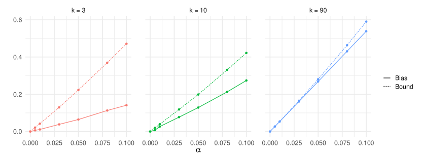
Figure 6: Comparison of the true bias and the bound in (33) for forward stepwise regression with $k=3$, 10, and 90 steps. The simulation setup is as in Section 5 with $s=5$ and $\mathrm{SNR}=2$.

F.2 Reducible variance

Now we examine the reducible variance empirically, and compare the bound in (36) in Proposition 4. We again use the simulation setup from Section 5, with $s=5$ and $\mathrm{SNR}=2$, with Figure 7 displays contour plots of the true reducible variance (computed via Monte Carlo) and the dominant term in (36) as functions of $B$ and $\alpha$, when $g$ is the lasso estimator with $\lambda=0.31$. The two panels appear qualitatively quite similar, confirming that the dominant term in (36) indeed captures the right dependence of the reducible variance on $B,\alpha$. (Note that each panel is given its own color scale, which means that any potential looseness in the constant multiplying $1/(B\alpha)$ in the bound (36) is not being reflected.)

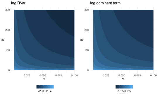
Figure 7: Comparison of the true reducible variance and the bound in (36) for the lasso with $\lambda=0.31$. The simulation setup is as in Section 5 with $s=5$ and $\mathrm{SNR}=2$.

F.3 Irreducible variance

Lastly, we examine the behavior of the irreducible variance and its components empirically. Following (39), observe that we can write

$$\mathrm{IVar}(\mathrm{CB}_{\alpha}(g))=\underbrace{\mathrm{Var}\big{(}\mathbb{E}\big{[}\|Y-g(Y+\sqrt{\alpha}\omega)\|_{2}^{2}\,\big{|}\,Y\big{]}\big{)}}_{\mathrm{IVar}_{1}}+\underbrace{\mathrm{Var}\bigg{(}\frac{2}{\sqrt{\alpha}}\mathbb{E}\big{[}\langle\omega,g(Y+\sqrt{\alpha}\omega)\rangle\,\big{|}\,Y\big{]}\bigg{)}}_{\mathrm{IVar}_{2}}+{}\\ \underbrace{2\mathrm{Cov}\bigg{(}\mathbb{E}\big{[}\|Y-g(Y+\sqrt{\alpha}\omega)\|_{2}^{2}\,\big{|}\,Y\big{]},\frac{2}{\sqrt{\alpha}}\mathbb{E}\big{[}\langle\omega,g(Y+\sqrt{\alpha}\omega)\rangle\,\big{|}\,Y\big{]}\bigg{)}}_{\mathrm{Cov}_{1,2}}.$$

We can similarly define analogous components for $\mathrm{IVar}_{1},\mathrm{IVar}_{2},\mathrm{Cov}_{1,2}$ for $\mathrm{IVar}(\mathrm{BY}_{\alpha}(g))$ in (43). Note that between the CB and BY estimators, $\mathrm{IVar}_{2}$ is shared (equal), but $\mathrm{IVar}_{1}$ and $\mathrm{Cov}_{1,2}$ are different: where BY uses the original training error $\|Y-g(Y)\|_{2}^{2}$, CB substitutes the conditional expectation of the noise-added training error $\mathbb{E}[\|Y-g(Y+\sqrt{\alpha}\omega)\|_{2}^{2}\,|\,Y]$.

Figure 8 plots these three components of the irreducible variance for BY and CB (computed via Monte Carlo), under the same simulation setup as that from Figure 2. The figure also plots the reducible variance for reference. We can see that the main contributor to the large variance exhibited by BY in comparison to CB in Figure 2 is in fact the first component of the irreducible variance $\mathrm{IVar}_{1}$. This is intuitive, because for an unstable function $g$ (such as the one in the current simulation), the observed training error can have a high degree of variability, but taking a conditional expectation over a noise-adding process acts as a kind of regularization, reducing this variability greatly.

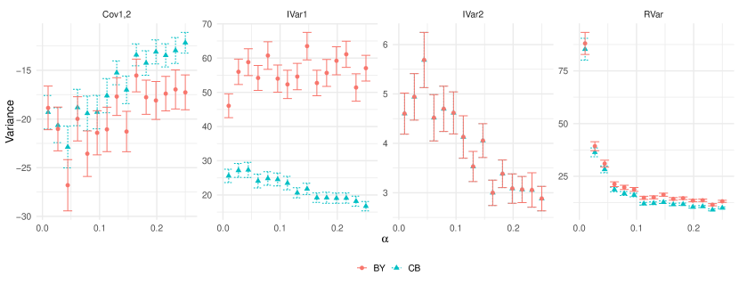
Figure 8: Comparison of the irreducible variance, broken down into its three main components, and also the reducible varaince, for the BY and CB estimators, under the same simulation setup as that in Figure 2.

References

• Akaike (1973) Hirotogu Akaike. Information theory and an extension of the maximum likelihood principle. In Second International Symposium on Information Theory, pages 267–281, 1973.
• Blu and Luisier (2007) Thierry Blu and Florian Luisier. The SURE-LET approach to image denoising. IEEE Transactions on Image Processing, 16(11):2778–2786, 2007.
• Breiman (1992) Leo Breiman. The little bootstrap and other methobds for dimensionality selection in regression: X-fixed prediction error. Journal of the American Statistical Association, 87(419):738–754, 1992.
• Cai (1999) T. Tony Cai. Adaptive wavelet estimation: A block thresholding and oracle inequality approach. Annals of Statistics, 27(3):898–924, 1999.
• Candes et al. (2013) Emmanuel J. Candes, Carlos M. Sing-Long, and Joshua D. Trzasko. Unbiased risk estimates for singular value thresholding and spectral estimators. IEEE Transactions on Signal Processing, 61(19):4643–4657, 2013.
• Chatterjee and Milanfar (2009) Priyam Chatterjee and Peyman Milanfar. Clustering-based denoising with locally learned dictionaries. IEEE Transactions on Image Processing, 18(7):1438–1451, 2009.
• Donoho and Johnstone (1995) David L. Donoho and Iain M. Johnstone. Adapting to unknown smoothness via wavelet shrinkage. Journal of the American Statistical Association, 90(432):1200–1224, 1995.
• Efron (1975) Bradley Efron. Defining the curvature of a statistical problem (with applications to second order efficiency). Annals of Statistics, 3(6):1189–1242, 1975.
• Efron (1986) Bradley Efron. How biased is the apparent error rate of a prediction rule? Journal of the American Statistical Association, 81(394):461–470, 1986.
• Efron (2004) Bradley Efron. The estimation of prediction error: Covariance penalties and cross-validation. Journal of the American Statistical Association, 99(467):619–632, 2004.
• Evans and Gariepy (2015) Lawrence C. Evans and Ronald F. Gariepy. Measure theory and fine properties of functions. CRC Press, 2015. Revised edition.
• Friedman et al. (2010) Jerome Friedman, Trevor Hastie, and Robert Tibshirani. Regularization paths for generalized linear models via coordinate descent. Journal of Statistical Software, 33(1):1–22, 2010.
• Hastie and Tibshirani (1990) Trevor Hastie and Robert Tibshirani. Generalized Additive Models. Chapman & Hall, 1990.
• Hastie et al. (2020) Trevor Hastie, Robert Tibshirani, and Ryan J. Tibshirani. Best subset, forward stepwise, or lasso? Analysis and recommendations based on extensive comparisons. Statistical Science, 35(4):579–592, 2020.
• Hoefling (2010) Holger Hoefling. A path algorithm for the fused lasso signal approximator. Journal of Computational and Graphical Statistics, 19(4):984–1006, 2010.
• Johnstone (1999) Iain M. Johnstone. Wavelet shrinkage for correlated data and inverse problems: Adaptivity results. Statistica Sinica, 9:51–83, 1999.
• Krishnan and Seelamantula (2014) Sunder R. Krishnan and Chandra S. Seelamantula. On the selection of optimum Savitzky-Golay filters. IEEE Transactions on Signal Processing, 61(2):380–391, 2014.
• Lingala et al. (2011) Sajan Goud Lingala, Yue Hu, Edward DiBella, and Mathews Jacob. Accelerated dynamic MRI exploiting sparsity and low-rank structure: k-t SLR. IEEE Transactions on Medical Imaging, 30(5):1042–1054, 2011.
• Mallows (1973) Colin Mallows. Some comments on $C_{p}$. Technometrics, 15(4):661–675, 1973.
• Metzler et al. (2016) Christopher A. Metzler, Arian Maleki, and Richard G. Baraniuk. From denoising to compressed sensing. IEEE Transactions on Information Theory, 62(9):5117–5144, 2016.
• Mikkelsen and Hansen (2018) Frederik Riis Mikkelsen and Niels Richard Hansen. Degrees of freedom for piecewise Lipschitz estimators. Annales de l’Institut Henri Poincaré Probabilités et Statistiques, 54(2):819–841, 2018.
• Ramani et al. (2008) Sathish Ramani, Thierry Blu, and Michael Unser. Monte-Carlo SURE: A black-box optimization of regularization parameters for general denoising algorithms. IEEE Transactions on Image Processing, 17(9):1540–1554, 2008.
• Rosset and Tibshirani (2020) Saharon Rosset and Ryan J. Tibshirani. From fixed-X to random-X regression: Bias-variance decompositions, covariance penalties, and prediction error estimation. Journal of the American Statistical Association, 15(529):138–151, 2020.
• Soltanayev and Chun (2018) Shakarim Soltanayev and Se Young Chun. Training deep learning based denoisers without ground truth data. In Advances in Neural Information Processing Systems, 2018.
• Stein (1981) Charles Stein. Estimation of the mean of a multivariate normal distribution. Annals of Statistics, 9(6):1135–1151, 1981.
• Stein and Weiss (1971) Elias M. Stein and Guido Weiss. Introduction to Fourier Analysis on Euclidean Spaces. Princeton University Press, 1971.
• Tian (2020) Xiaoying Tian. Prediction error after model search. Annals of Statistics, 48(2):763–784, 2020.
• Tibshirani et al. (2005) Robert Tibshirani, Michael Saunders, Saharon Rosset, Ji Zhu, and Keith Knight. Sparsity and smoothness via the fused lasso. Journal of the Royal Statistical Society: Series B, 67(1):91–108, 2005.
• Tibshirani (2015) Ryan J. Tibshirani. Degrees of freedom and model search. Statistica Sinica, 25(3):1265–1296, 2015.
• Tibshirani and Rosset (2019) Ryan J. Tibshirani and Saharon Rosset. Excess optimism: How biased in the apparent error rate of a SURE-tuned prediction rule? Journal of the American Statistical Association, 114(526):697–712, 2019.
• Tibshirani and Taylor (2011) Ryan J. Tibshirani and Jonathan Taylor. The solution path of the generalized lasso. Annals of Statistics, 39(3):1335–1371, 2011.
• Tibshirani and Taylor (2012) Ryan J. Tibshirani and Jonathan Taylor. Degrees of freedom in lasso problems. Annals of Statistics, 40(2):1198–1232, 2012.
• Ulfarsson and Solo (2013a) Magnus O. Ulfarsson and Victor Solo. Tuning parameter selection for nonnegative matrix factorization. In Proceedings of the IEEE International Conference on Acoustics, Speech and Signal Processing, 2013a.
• Ulfarsson and Solo (2013b) Magnus O. Ulfarsson and Victor Solo. Tuning parameter selection for underdetermined reduced-rank regression. IEEE Signal Processing Letters, 20(9):881–884, 2013b.
• Wang and Morel (2013) Yi-Qing Wang and Jean-Michel Morel. SURE guided gaussian mixture image denoising. SIAM Journal of Imaging Sciences, 6(2):999–1034, 2013.
• Ye (1998) Jianming Ye. On measuring and correcting the effects of data mining and model selection. Journal of the American Statistical Association, 93(441):120–131, 1998.
• Zou and Yuan (2008) Hui Zou and Ming Yuan. Regularized simultaneous model selection in multiple quantiles regression. Computational Statistics and Data Analysis, 52(12):5296–5304, 2008.
• Zou et al. (2007) Hui Zou, Trevor Hastie, and Robert Tibshirani. On the “degrees of freedom" of the lasso. Annals of Statistics, 35(5):2173–2192, 2007.