Abstract

We study the effects of a magnetic field on the chaotic dynamics of a string with endpoints on the boundary of an asymptotically AdS₅ space with black hole. We study Poincaré sections and compute the Lyapunov exponents for the string perturbed from the static configuration, for two different orientations, with position of the endpoints on the boundary orthogonal and parallel to the magnetic field. We find that the magnetic field stabilizes the string dynamics, with the largest Lyapunov exponent remaining below the Maldacena-Shenker-Stanford bound.

1 Introduction

The aim of this paper is to study the effect of a constant and uniform magnetic field on the chaotic behavior of a suspended string in a gravitational background. Among others, one purpose is to scrutinize the stabilization role of the magnetic field for different orientations of the string. The study follows the tests, carried out using holographic methods, of the Maldacena-Shenker-Stanford (MSS) bound [1]. This conjectures, under general conditions, that for a thermal quantum system at temperature $T$ some out-of-time-ordered correlation functions involving Hermitian operators have an exponential time dependence in determined time intervals. The dependence is characterized by the exponent $\lambda$, and for such an exponent an upper bound (written in units where $\hbar=1$ and $k_{B}=1$) holds:

$$\lambda\leqslant 2\pi T.$$ (1)

The correlation functions are related to thermal expectation values of the squared commutator of two Hermitian operators at a time separation $t$, which quantify the effect of one operator on measurements of the other one at a later time.

The MSS bound has been inspired by the observation that in nature the black holes (BH) are the fastest “scramblers”: the time needed for a system near a BH horizon to loose information depends logarithmically on the number of the system degrees of freedom [2, 3]. Connections between chaotic quantum systems and gravity have been investigated in [4, 5, 6, 7]. In a holographic framework, a relation has been worked out between the size of the operators of the quantum theory on the boundary, which are involved in the temporal evolution of the perturbation, and the momentum of a particle falling in the bulk [8, 9].

Holographic methods have been used to challenge the MSS bound (1). In such studies the quantum system is conjectured to be a $4d$ boundary theory dual to an AdS₅ gravity theory with a black hole [10, 11, 12]. Several investigations are described in [13, 14, 15, 16]. Some studies concern strings hanging in the bulk with endpoints on the boundary, which are the holographic dual of a static quark-antiquark pair [17, 18, 19, 20]. In such systems $\lambda$ is the Lyapunov exponent characterizing the chaotic behavior of the fluctuations around the static string configuration [21, 22, 23]. The studies include the case of quantum systems characterized by a global $U(1)$ symmetry, and show that the chemical potential stabilizes the chaotic dynamics [24].

It is interesting to consider the role of an external magnetic field on the chaotic behaviour of the string. The magnetic field is relevant in different contexts, including heavy-ion collisions or condensed matter problems such as the Quantum Hall Effect and superconductivity at high temperatures. A general gravity dual for such systems should include a magnetic field [25, 26, 27, 28, 29]. The backreaction of an external magnetic field modifies the geometry of the $5d$ spacetime, the metric of which is determined by the Einstein equations. As a result, an anisotropy is introduced in the spatial directions. Moreover, in a finite temperature system the relation between the position of the black-hole horizon, the source of chaos in the $5d$ geometry, and temperature, involved in the MSS relation in the boundary theory, is modified by the magnetic field.

In this paper we aim at studying how the background magnetic field affects chaos for the hanging string, how this depends on the string orientation, and if the MSS bound is satisfied.

2 Geometry with a magnetic field

In the gauge/gravity duality, a $4d$ boundary gauge theory at finite temperature is dual to a gravity theory in AdS₅ with a black hole. A magnetic field is introduced in the holographic framework by a $U(1)$ gauge field $F_{MN}$ which modifies the $5d$ geometry. The metric is determined solving the Einstein equations:

$$R_{MN}-\frac{1}{2}g_{MN}(R+12)-T_{MN}=0$$ (2)

with the $5d$ stress-energy tensor

$$T_{MN}=2\,(g^{AB}F_{MA}F_{NB}-\frac{1}{4}g_{MN}F^{2})\,.$$ (3)

For a constant magnetic field $B$ in the $x_{3}$ direction $F$ is given by $F=B\,dx^{1}\wedge dx^{2}$, hence the only nonvanishing components are $F_{12}=-F_{21}=B$. The Einstein equations have been solved perturbatively in the low-$B$ and high temperature limits in Refs.[30, 31, 32]. The result for the line element, having the general expression

$$ds^{2}=g_{tt}dt^{2}+g_{11}(dx^{1})^{2}+g_{22}(dx^{2})^{2}+g_{33}(dx^{3})^{2}+g_{rr}dr^{2}$$ (4)

with $r>r_{h}$, reads:

$$g_{tt}=-r^{2}f(r),\quad g_{11}=g_{22}=r^{2}h(r),\quad g_{33}=r^{2}q(r),\quad g_{rr}=\frac{1}{r^{2}f(r)}.$$ (5)

The metric functions are [32]:

$$f(r) = 1-\frac{2B^{2}}{3r^{4}}\log r+\frac{f_{4}}{r^{4}}$$ (6)

$$q(r) = 1-\frac{2B^{2}}{3r^{4}}\log r$$ (7)

$$h(r) = 1+\frac{B^{2}}{3r^{4}}\log r\,.$$ (8)

The magnetic field breaks rotational invariance, hence $g_{22}\neq g_{33}$. The geometry has a horizon, the position of which $r_{h}$ is found requiring $f(r_{h})=0$. This gives $\displaystyle f_{4}=-r_{h}^{4}+\frac{2}{3}\,B^{2}\log(r_{h})$ and the blackening function $f(r)$:

$$f(r)=1-\frac{r_{h}^{4}}{r^{4}}-\frac{2B^{2}}{3r^{4}}\log{\frac{r}{r_{h}}}.$$ (9)

The Hawking temperature $T$ depends on the magnetic field:

$$T=\frac{r_{h}}{\pi}\left(1-\frac{B^{2}}{6r_{h}^{4}}\right)\,.$$ (10)

The metric given in terms of the functions (6)-(8) is obtained for large bulk coordinate $r$ and low $B$, and it is important to reckon the minimum value of $r$ and the largest value of $B$ for which it is a good approximation of Eqs. (2),(3) and (5). In Fig. 1 the differences between the metric functions $f(r)$, $q(r)$ and $h(r)$ in (6)-(8) and the corresponding ones computed for low $B$ in [30, 31] and used in [33] are depicted setting $r=1.1$ and varying $B$. The comparison shows that the largest deviation between the two expressions of the metric, resulting from the different approximations in determining the solution of the Einstein equations, is in the function $q$. For larger values of the coordinate $r$ the deviations are smaller.

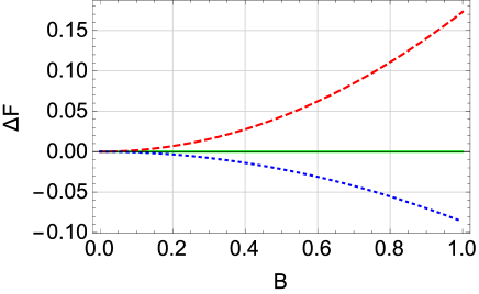
Figure 1: For $F$ one of the metric functions $f(r=1.1)$ (green line), $q(r=1.1)$ (red dashed line) and $h(r=1.1)$ (blue dotted line), $\Delta F$ is the difference between each function in Eqs. (6)-(8) and the corresponding one computed in Ref.[30, 31, 33], for $r_{h}=1$ and varying the magnetic field $B$.

In Fig. 2 the differences between the metric functions in (6)-(8) and the ones obtained by a numerical solution of the Einstein equations are depicted for the same value $r=1.1$, varying the magnetic field $B$. The numerical solutions are obtained imposing as boundary conditions for $r\to\infty$ the asymptotic expansion in (6)-(8), plus additional terms up to $\mathcal{O}(1/r^{8}$). The parameter $f_{4}$ in the asymptotic functions is fixed imposing $f(r_{h})=0$. The deviations between (6)-(8) and those in Refs.[30, 31, 33] are larger because in such references different conditions for $q(r_{h})$ and $h(r_{h})$ are imposed.

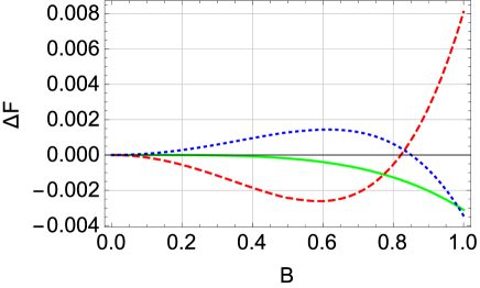
Figure 2: For $F$ one of the metric functions $f(r=1.1)$ (green line), $q(r=1.1)$ (red dashed line) and $h(r=1.1)$ (blue dotted line), $\Delta F$ is the difference between each function in (6)-(8) and the one numerically computed from the Einstein equations, for $r_{h}=1$ and varying the magnetic field $B$.

In view of this comparison, in our study the magnetic field is increased up to $B=1$. For the radial coordinate $r$, setting the horizon position $r_{h}=1$ in all our study, we consider $r\geqslant 1.1$.

3 String profile in the gravitational background

We consider a string described by the functions $r(t,\ell)$ and $x_{i}(t,\ell)$, with fixed endpoints on the AdS boundary $r\to\infty$. We consider two configurations, $i=1$ and $i=3$. In the former (latter) configuration the string endpoints lie on a line orthogonal (parallel) to the magnetic field. $(t,\ell)$ are the worldsheet coordinates, with $\ell$ the proper distance measured along the string. In the probe approximation we ignore the backreaction to the metric (4)-(8).

The string dynamics is governed by the Nambu-Goto (NG) action:

$$\mathcal{S}=-\frac{1}{2\pi\alpha^{\prime}}\int dt\,d\ell\,\sqrt{-h}\,,$$ (11)

where $\alpha^{\prime}$ is the string tension and $h$ is the determinant of the induced metric $h_{ij}=g_{MN}\frac{\partial X^{M}}{\partial\xi_{i}}\frac{\partial X^{N}}{\partial\xi_{j}}$, with $\xi_{i,j}$ the worldsheet coordinates and $g$ the metric tensor (5). In the static case the action reads:

$$\mathcal{S}=-\frac{T}{2\pi\alpha^{\prime}}\int d\ell\,\sqrt{|g_{tt}g_{ii}{\acute{x}_{i}}^{2}+g_{tt}g_{rr}{\acute{r}}^{2}|}\,,$$ (12)

where $\acute{x}$ denotes the derivative with respect to $\ell$. $x_{i}$ is a cyclic coordinate, so its conjugate momentum

$$\frac{\partial\mathcal{L}}{\partial\acute{x}_{i}}=-\frac{T}{2\pi\alpha^{\prime}}\frac{|g_{tt}|g_{ii}{\acute{x}_{i}}}{\sqrt{|g_{tt}|g_{ii}{\acute{x}_{i}}^{2}+|g_{tt}|g_{rr}{\acute{r}}^{2}}}$$ (13)

is a constant of motion. Denoting with $r(\ell=0)=r_{0}$ the position of the tip of the string in the bulk, i.e. the point where $\displaystyle\frac{dr}{dx_{i}}\Big{|}_{\ell=0}=0$, we have:

$$\frac{\sqrt{|g_{tt}|}g_{ii}{\acute{x}_{i}}}{\sqrt{g_{ii}{\acute{x}_{i}}^{2}+g_{rr}{\acute{r}}^{2}}}=\left.\sqrt{|g_{tt}|g_{ii}}\right|_{\ell=0}\,.$$ (14)

Moreover, from the condition

$$d\ell^{2}=g_{ii}\,dx_{i}^{2}+g_{rr}\,dr^{2}$$ (15)

the equations determining the string profile can be obtained:

$$\acute{x}=\pm\frac{\sqrt{-g_{tt}(r_{0})g_{ii}(r_{0})}}{\sqrt{-g_{tt}}g_{ii}}$$ (16)

$$\acute{r}=\pm\frac{\sqrt{-g_{tt}g_{ii}+g_{tt}(r_{0})g_{ii}(r_{0})}}{\sqrt{-g_{tt}g_{ii}g_{rr}}}\,.$$ (17)

We set as boundary conditions that the string endpoints lie on the AdS₅ boundary at $x_{i}=\pm L/2$. The minimum value $r_{0}$ of the coordinate $r$ is reached at $x_{i}=0$ (or $\ell=0$). $L$ and $r_{0}$ are related, since

$$L=2\int_{r_{0}}^{\infty}dr\,\Bigg{(}\frac{g_{ii}(r)}{g_{rr}(r)}\left(\frac{g_{tt}(r)g_{ii}(r)}{g_{tt}(r_{0})g_{ii}(r_{0})}-1\right)\Bigg{)}^{-\frac{1}{2}}\,.$$ (18)

The function $L(r_{0})$ with $B=1$ is plotted in Fig. 3. It has a maximum separating unstable strings (red dotted line in the figure), corresponding to positive energies, from metastable (blue dashed line) and stable strings (black solid line) corresponding to negative energies [24]. In the following we focus on the unstable string solutions, varying the magnetic field in the range $B\leqslant 1$.

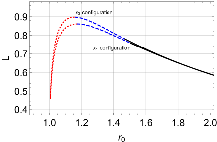
Figure 3: Distance between the string endpoints on the boundary vs the position of the tip of the string, obtained using Eq. (18) with $r_{h}=1$ and $B=1$, for the two string configurations.

4 Perturbing the static solution

To observe the onset of chaos the static solution of the string near the black-hole horizon must be perturbed by a small time-dependent effect.

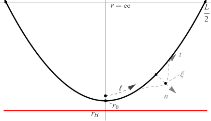
Figure 4: Static string profile, and perturbation $\xi(t,\ell)$ along the direction orthogonal to the string in each point having coordinate $\ell$.

We introduce a perturbation of the string along the orthogonal direction at each point with coordinate $\ell$ in the $r-x$ plane, for both the $x=x_{1}$ and $x=x_{3}$ configurations [21, 24]. The perturbation is depicted in Fig. 4. Considering the unit vector $n^{M}=(0,n^{x},0,0,n^{r})$ orthogonal to $t^{M}$, we have:

$$g_{rr}(r)\left({n}{{}^{r}}\right)^{2}+g_{xx}(r)\left({n}{{}^{x}}\right)^{2} = 1$$ (19)

$$\acute{r}\left(\ell\right)g_{rr}\left(r\right)\,n^{r}+\acute{x}\left(\ell\right)g_{xx}\left(r\right)\,n^{x} = 0\,.$$ (20)

For an outward perturbation as in Fig. 4 the solution for the components $n^{x}$ and $n^{r}$ is

$${n^{x}}(\ell)=\sqrt{\frac{g_{rr}}{g_{xx}}}\;\acute{r}(\ell)\quad\text{,}\quad{n}{{}^{r}}(\ell)=-\sqrt{\frac{g_{xx}}{g_{rr}}}\;\acute{x}(\ell)\quad.$$ (21)

The time-dependent perturbation $\xi\left(t,\ell\right)$ modifies $r$ and $x$:

$$r\left(t,\ell\right) = r_{BG}\left(\ell\right)+\xi\left(t,\ell\right)n^{r}\left(\ell\right),$$

$$x\left(t,\ell\right) = x_{BG}\left(\ell\right)+\xi\left(t,\ell\right)n^{x}\left(\ell\right),$$

where $r_{BG}\left(\ell\right)$ and $x_{BG}\left(\ell\right)$ are the static solutions obtained integrating Eqs. (16) and (17).

To describe the dynamics of the small perturbation, we expand the metric function around the static solution $r_{BG}(\ell)$ to the third order in $\xi\left(t,\ell\right)$. To this order in $\xi$ the NG action comprises a quadratic and a cubic term. The quadratic term has the form:

$$S^{\left(2\right)}=\frac{1}{2\pi\alpha^{\prime}}\int\mathrm{d}t\int_{-\infty}^{\infty}\mathrm{d}\ell\left(C_{tt}^{x_{i}}\dot{\xi}^{2}+C_{\ell\ell}^{x_{i}}\acute{\xi}^{2}+C_{00}^{x_{i}}\xi^{2}\right)\qquad\qquad(i=1,3)$$ (22)

for the two chosen string orientations. $C_{tt}^{x_{i}}$, $C_{\ell\ell}^{x_{i}}$ and $C_{00}^{x_{i}}$ depend on $\ell$. For the geometry in Eq. (4) with metric functions $f(r)$, $h(r)$ and $q(r)$ the coefficients $C_{tt}^{x_{i}}$, $C_{\ell\ell}^{x_{i}}$ and $C_{00}^{x_{i}}$ read:

$$C_{tt}^{x_{i}}\left(\ell\right) =\frac{1}{2r_{BG}\sqrt{f\left(r_{BG}\right)}},$$ (23)

$$C_{\ell\ell}^{x_{i}}\left(\ell\right) =-\frac{1}{4C_{tt}^{x_{i}}\left(\ell\right)},$$

$$C_{00}^{x_{1}}\left(\ell\right) =\frac{1}{8r_{BG}^{3}f(r_{BG})^{3/2}h(r_{BG})^{2}}\Big{(}\bigl{(}r_{0}^{4}f(r_{0})h(r_{0})\bigl{(}2r_{BG}^{2}h(r_{BG})f^{\prime}(r_{BG})^{2}$$

$$+2f(r_{BG})^{2}\bigl{(}4h(r_{BG})+r_{BG}h^{\prime}(r_{BG})\bigr{)}+r_{BG}f(r_{BG})\bigl{(}r_{BG}f^{\prime}(r_{BG})h^{\prime}(r_{BG})$$

$$+2h(r_{BG})\bigl{(}f^{\prime}(r_{BG})-r_{BG}f^{\prime\prime}(r_{BG})\bigr{)}\bigr{)}\bigr{)}-r_{BG}^{4}f(r_{BG})^{2}\bigl{(}2r_{BG}h(r_{BG})f^{\prime}(r_{BG})$$

$$\bigl{(}2h(r_{BG})+r_{BG}h^{\prime}(r_{BG})\bigr{)}+f(r_{BG})\bigl{(}8h(r_{BG})^{2}-r_{BG}^{2}h^{\prime}(r_{BG})^{2}$$

$$+2r_{BG}h(r_{BG})\bigl{(}4h^{\prime}(r_{BG})+r_{BG}h^{\prime\prime}(r_{BG})\bigr{)}\bigr{)}\bigr{)}\Bigr{)}.$$

$C_{00}^{x_{3}}$ has the same expression of $C_{00}^{x_{1}}$, with the metric function $h(r)$ replaced by $q(r)$. The coefficients depend on $\ell$ through $r_{BG}\left(\ell\right)$. The metric functions $f(r)$, $h(r)$ and $q(r)$ are defined in Eqs. (6)-(8).

The equation of motion from the action (22) is

$$\qquad\qquad C_{tt}^{x_{i}}\,\ddot{\xi}+\partial_{\ell}\left(C_{\ell\ell}^{x_{i}}\acute{\xi}\right)-C_{00}^{x_{i}}\,\xi=0\qquad\qquad\qquad(i=1,3).$$ (24)

Factorizing $\xi\left(t,\ell\right)=\xi\left(\ell\right)e^{i\omega t}$ it corresponds to the Sturm-Liouville equation

$$\partial_{\ell}\left(C_{\ell\ell}^{x_{i}}\,\acute{\xi}\right)-C_{00}^{x_{i}}\,\xi=\omega^{2}C_{tt}^{x_{i}}\,\xi\,\,,$$ (25)

with $W(\ell)=-C_{tt}^{x_{i}}(\ell)$ the weight function. We solve Eq. (25) for different values of $B$. Since we are interested in unstable configurations we set $r_{0}=1.1$ near the horizon, and impose the boundary conditions $\xi\left(\ell\right)\xrightarrow{\ell\rightarrow\pm\infty}0$. The two lowest lying eigenvalues $\omega_{0}^{2}$ and $\omega_{1}^{2}$, obtained varying $B$ for the two different string configurations, are collected in Table 1. The corresponding eigenfunctions $\xi\left(\ell\right)=e_{0}\left(\ell\right)$ and $\xi\left(\ell\right)=e_{1}\left(\ell\right)$, for one configuration of the string, are depicted in Fig. 5.

$x_{1}$ configuration				$x_{3}$ configuration
$B$	$\omega_{0}^{2}$	$\omega_{1}^{2}$		$B$	$\omega_{0}^{2}$	$\omega_{1}^{2}$
0	-1.370	7.638		0	-1.370	7.638
0.3	-1.327	7.531		0.3	-1.317	7.548
0.6	-1.202	7.213		0.6	-1.166	7.278
0.9	-1.004	6.694		0.9	-0.932	6.823
1	-0.923	6.478		1	-0.841	6.629

Table 1: Eigenvalues $\omega_{0}^{2}$ and $\omega_{1}^{2}$ of Eq. (25) for $r_{0}=1.1$ and varying $B$, for the two string configurations.

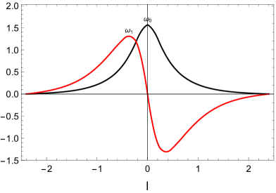
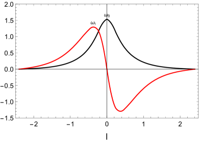
Figure 5: Eigenfunctions $e_{0}\left(\ell\right)$ (black line) and $e_{1}\left(\ell\right)$ (red line) of Eq. (25), for $r_{0}=1.1$ and $B=0$ (left), $B=0.6$ (right panel).

Negative eigenvalues corrispond to unstable systems. Considering the results in Table 1, we conclude that the effect of $B$ is to stabilize the system, since $\omega_{0}^{2}$ increases with $B$. The effect of the magnetic field $B$ is stronger for the string in the $x_{3}$ direction, parallel to the magnetic field, hence the magnetic field stabilizes the system in the $x_{3}$ configuration more than in the $x_{1}$ configuration.

To observe the chaotic behaviour we study the contribution of the third order terms in $\xi$ in the action. Up to a surface term, the expression is

$$S^{\left(3\right)}=\frac{1}{2\pi\alpha^{\prime}}\int\mathrm{d}t\int_{-\infty}^{\infty}\mathrm{d}\ell\bigg{\{}D_{0}\,\xi^{3}+D_{1}^{x_{i}}\,\xi\acute{\xi}^{2}+D_{2}^{x_{i}}\,\xi\dot{\xi}^{2}\bigg{\}}\,\,,$$ (26)

with $D_{0,1,2}^{x_{i}}$ functions of $\ell$. Expanding the perturbation in terms of the first two eigenfunctions $e_{0}$ and $e_{1}$,

$$\xi\left(t,\ell\right)=c_{0}\left(t\right)e_{0}\left(\ell\right)+c_{1}\left(t\right)e_{1}\left(\ell\right),$$ (27)

the time dependence of the perturbation is encoded in the coefficients $c_{0}(t)$ and $c_{1}(t)$. With this form of $\xi(t,\ell)$ we have:

$$S^{\left(3\right)}=$$

$$\frac{1}{2\pi\alpha^{\prime}}\int\mathrm{d}t\int_{-\infty}^{\infty}\mathrm{d}\ell\Big{[}\Big{(}D_{0}^{x_{i}}\,e_{0}^{3}+D_{1}^{x_{i}}\,e_{0}\acute{e}_{0}^{2}\Big{)}c_{0}^{3}\left(t\right)+\Big{(}3D_{0}^{x_{i}}\,e_{0}e_{1}^{2}+D_{1}^{x_{i}}\left(2\acute{e}_{0}e_{1}\acute{e}_{1}+e_{0}\acute{e}_{1}^{2}\right)\Big{)}c_{0}c_{1}^{2}$$

$$+D_{2}^{x_{i}}\Big{(}e_{0}e_{1}^{2}c_{0}\dot{c}_{1}^{2}+e_{0}^{3}e_{1}^{2}c_{0}\dot{c}_{0}^{2}+2e_{0}e_{1}^{2}\dot{c}_{0}c_{1}\dot{c}_{1}\Big{)}\Big{]}.$$ (28)

The action for $c_{0}(t)$ and $c_{1}(t)$ is obtained by the sum $S^{(2)}+S^{(3)}$, integrating over $\ell$:

$$S^{(2)}+S^{(3)}=\frac{1}{2\pi\alpha^{\prime}}\int\mathrm{d}t\Big{[}\sum_{n=0,1}\left(\dot{c}_{n}^{2}-\omega_{n}^{2}c_{n}^{2}\right)+K_{1}^{x_{i}}c_{0}^{3}+K_{2}^{x_{i}}c_{0}c_{1}^{2}+K_{3}^{x_{i}}c_{0}\dot{c}_{0}^{2}+K_{4}^{x_{i}}c_{0}\dot{c}_{1}^{2}+K_{5}^{x_{i}}\dot{c}_{0}c_{1}\dot{c}_{1}\Big{]}.$$ (29)

In Eqs. (26)-(29) the index is $i=1$ or $i=3$. The coefficients $K_{1,\dots,5}^{x_{i}}$ depend on $r_{0}$ and $B$. They are collected in Tab. 2 for $r_{0}=1.1$ and different values of $B$, for the two string configurations.

$x_{1}$ configuration
	$B$	$K_{1}$	$K_{2}$	$K_{3}$	$K_{4}$	$K_{5}$
	0	11.36	21.72	10.58	3.37	6.73
	0.3	10.89	21.17	10.50	3.36	6.72
	0.6	9.57	19.56	10.24	3.33	6.67
	0.9	7.63	17.05	9.83	3.29	6.58
	1	6.90	16.05	9.65	3.27	6.55
$x_{3}$ configuration
	$B$	$K_{1}$	$K_{2}$	$K_{3}$	$K_{4}$	$K_{5}$
	0	11.36	21.72	10.58	3.37	6.73
	0.3	10.97	21.22	10.52	3.37	6.74
	0.6	9.85	19.76	10.32	3.38	6.77
	0.9	8.16	17.44	9.99	3.41	6.81
	1	7.50	16.50	9.85	3.41	6.83

Table 2: $K_{i}$ coefficients in Eq. (29) for the two string configurations, for $r_{0}=1.1$ and varying the magnetic field $B$.

The potential described by Eq. (29) has a trap for the unstable string configurations. We are interested in the motion of $c_{0}$ and $c_{1}$ in the trap. In some regions of the potential the kinetic term is negative. As shown in [21, 24], it is useful to replace $c_{0,1}\to\tilde{c}_{0,1}$ in the action, with $c_{0}=\tilde{c}_{0}+\alpha_{1}\tilde{c}_{0}^{2}+\alpha_{2}\tilde{c}_{1}^{2}$ and $c_{1}=\tilde{c}_{1}+\alpha_{3}\tilde{c}_{0}\tilde{c}_{1}$, neglecting $\mathcal{O}\left(\tilde{c}_{i}^{4}\right)$ terms, setting the constants $\alpha_{i}$ ensuring the positivity of the kinetic term. We set $\alpha_{1}=-2$, $\alpha_{2}=-0.5$ and $\alpha_{3}=-1$. This replacement stretches the potential and stabilizes the time evolution of the system. The dynamics is not affected, and a chaotic behaviour shows up also in the transformed system.

5 Poincaré sections and Lyapunov exponents

The onset of chaos is displayed by the Poincaré sections. We construct the sections defined by $\tilde{c}_{1}\left(t\right)=0$ and $\dot{\tilde{c}}_{1}\left(t\right)\geqslant 0$ for bounded orbits within the trap in the potential. For $r_{0}=1.1$ and increasing $B$ the sections are depicted in Fig. 6. For $\tilde{c}_{0}$ near zero the orbits are scattered points which depend on the initial conditions. Increasing $B$ the points in the sections form more regular paths, showing that the effect of switching on the magnetic field is to mitigate the chaotic behavior.

         

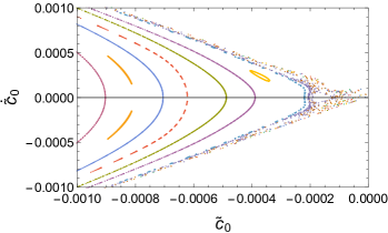
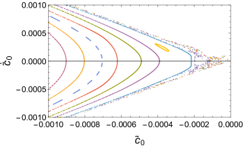
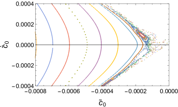
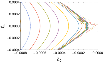
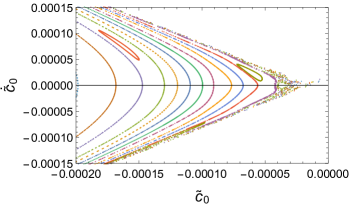
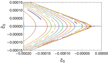
Figure 6: Poincaré sections for a perturbed string in the $x_{1}$ (left column) and $x_{3}$ configurations (right column). The initial conditions are changed with fixed energy $E=10^{-5}$ and $r_{0}=1.1$. The magnetic field is increased from $B=0.3$ (top row) to $B=0.6$ (middle row) and $B=1$ (bottom row). The sections correspond to $\tilde{c}_{1}=0$ and $\dot{\tilde{c}}_{1}\geqslant 0$.

In Fig. 6 we observe that when the string is along $x_{3}$ we need to go closer to $\tilde{c}_{0}=0$, closer to the horizon, to observe chaos. This confirms the observation that the strongest stabilization effect of the magnetic field is in the $x_{3}$ configuration.

For a better understanding of the amount of chaos we evaluate the Lyapunov exponents. Such exponents in the four dimensional $c_{0}$, $c_{1}$ phase-space can be computed for different values of $B$ using the numerical method described in [34]. The results are shown in Fig. 7.

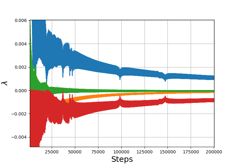
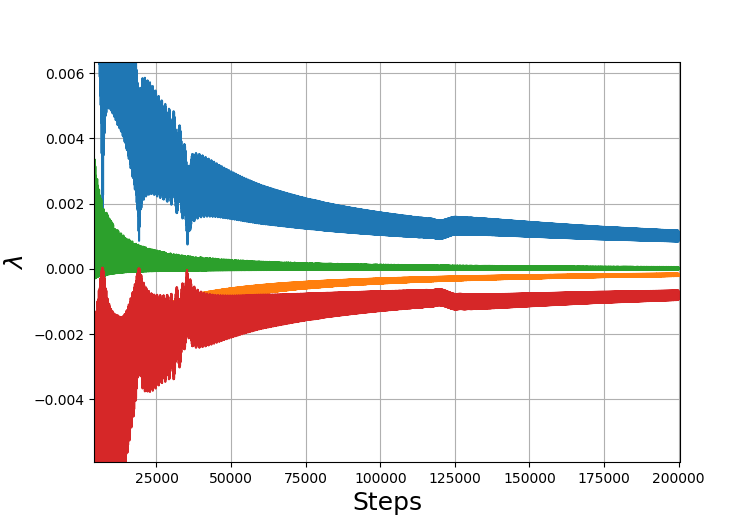
Figure 7: Convergency plots of the four Lyapunov exponents for a string along $x_{1}$, with $r_{0}=1.1$ and $B=0.3$ (right panel), $B=0.6$ (left panel). $2\times 10^{5}$ time steps are shown. For the initial conditions, the energy is set to $E=10^{-5}$ together with $\tilde{c}_{0}=-0.0002$, $\dot{\tilde{c}}_{0}=0$, $\tilde{c}_{1}=0.0011$.

The convergency plot is a damped oscillating function. The value of the largest Lyapunov exponent can be extrapolated fitting the maximum in each oscillation and considering $t\to+\infty$. The values obtained from the fit decrease as $B$ increases, as shown in Fig. 8: the effect of the magnetic field is to soften the dependence on the initial conditions, making the string less chaotic. In the numerical procedure it is checked that the sum of the Lyapunov exponents vanishes at large $t$.

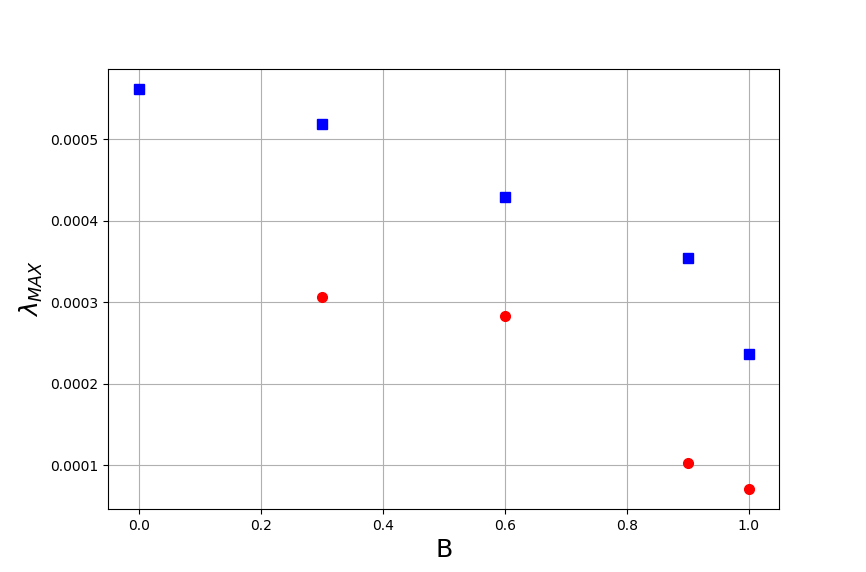
Figure 8: Largest Lyapunov exponent $\lambda_{MAX}$ versus $B$ for $r_{0}=1.1$. The results for the $x_{1}$ (blue points) and $x_{3}$ string configurations (red points) are shown.

In Fig. 8 the results for the two configurations are compared. For the same values of $B$ and $r_{0}$, so at the same distance from the BH horizon, smaller Lyapunov exponents are found in the $x_{3}$ configuration.

The Poincaré plots show that chaos is produced in the proximity of the BH horizon, and that the string dynamics is less chaotic if the magnetic field increases. This is confirmed by the largest Lyapunov exponent. The effect of the BH horizon can be observed looking at the first steps of the Lyapunov convergency plots shown in Fig. 9. In the early times, as long as the system is inside a region near $\tilde{c}_{0}\sim 0$, the exponents approach a nearly constant value. When the system is far from the origin, they begin to oscillate and drop to a lower asymptotic value shown in Fig. 7. This early time behavior is observed when in general the trajectory crosses a chaotic region of the phase-space. If initial conditions are of a trajectory that does not come close to the origin, such a behavior is not observed. For the time evolution of the convergency plots stopped before the plateaux start decreasing, higher values of the largest Lyapunov exponents with respect to the asymptotic ones in Fig. 8 would be found. The snapshot of the time evolution near the BH horizon shown in Fig. 9 further shows that the BH horizon is the source of chaos. The role of the magnetic field to stabilize the system is also displayed by the early time behaviour.

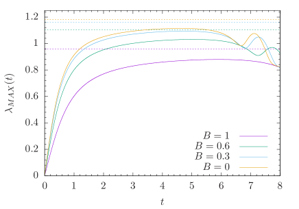
Figure 9: Early time convergency plots of the largest Lyapunov exponent, for the $x_{1}$ configuration, $r_{0}=1.1$ and $B$ indicated in the legend. The energy is set to $E=10^{-5}$, with the initial conditions $\tilde{c}_{0}=-0.0002$, $\dot{\tilde{c}}_{0}=0$ and $\tilde{c}_{1}=0.0011$. The dashed lines show the largest Lyapunov exponents at the saddle point discussed in Sec. 6.

6 Analysis of the saddle point

In the previous section we have computed the Lyapunov exponents of an extended bounded orbit in the phase space, and we have obtained positive values for the largest Lyapunov exponents proving that the system is chaotic. In order to complete the analysis of Lyapunov exponents and challenge the MSS bound, in this section we compute the Lyapunov exponents at the unstable fixed point. However, we remark that the sign of the largest Lyapunov exponent at the fixed point only indicates the stability of that point (it is positive for unstable fixed points), but it carries no information about the dynamics of the whole system and cannot be used to argue if the system is chaotic.

The evolution of the system governed by the action in Eq. (29) is dictated by the equation $\dot{\vec{x}}=\vec{F}$, with $\vec{x}=(\tilde{c}_{0},\dot{\tilde{c}}_{0},\tilde{c}_{1},\dot{\tilde{c}}_{1})$. There are two fixed points where $\vec{F}=0$: a stable fixed point corresponding to the local minimum of the potential obtained from Eq. (29), and an unstable fixed point corresponding to the saddle point of the potential, shown in Fig. 10 for a set of parameters.

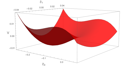
Figure 10: Potential obtained from Eq. (29) for $B=1$.

If an unstable unperturbed string is chosen as solution of Eqs. (16)-(17), for the energy $E=0$ the unstable fixed point is at $\vec{x}=(0,0,0,0)$. At a fixed point the formula defining the Lyapunov exponents gets simpler [34], and they can be computed analytically as the real part of the eigenvalues of the Jacobian matrix of $\vec{F}$. At the point $(0,0,0,0)$ this Jacobian reads:

$$J=\left(\begin{array}[]{cccc}0&-\omega_{0}^{2}&0&0\\ 1&0&0&0\\ 0&0&0&-\omega_{1}^{2}\\ 0&0&1&0\end{array}\right)\,,$$ (30)

and its eigenvalues are $(-i\sqrt{\omega_{0}^{2}},i\sqrt{\omega_{0}^{2}},-i\sqrt{\omega_{1}^{2}},i\sqrt{\omega_{1}^{2}})$. Hence, the Lyapunov exponents vanish for $\omega_{i}^{2}>0$, as for stable solutions. Fig. 11 shows the largest Lyapunov exponents $\lambda_{MAX}=\sqrt{-\omega_{0}^{2}}$ at the fixed point $(0,0,0,0)$, for $B=1$ and varying $r_{0}$. In Fig. 12 the exponents are plotted as a function of $B$ for $r_{0}=1.1$. The values of the Lyapunov exponent at this point are large, but they remain below the MSS bound $\lambda_{MSS}=2r_{h}\left(1-\frac{B^{2}}{6r_{h}^{4}}\right)$ (dashed line in the plots) when the string tip gets close to the black hole horizon, $r_{0}\to r_{h}$. As a final check, in Fig. 13 it is shown that the Lyapunov exponents computed at the fixed point $(0,0,0,0)$ by the numerical procedure of Ref. [34] used in the previous section, are equal to the analytical ones $(\sqrt{-\omega_{0}^{2}},-\sqrt{-\omega_{0}^{2}},0,0)$.

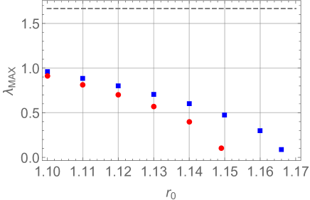
Figure 11: Largest Lyapunov exponent at the unstable fixed point $(0,0,0,0)$, as a function of $r_{0}$, for $B=1$. The blue (red) points refer to the $x_{1}$ ($x_{3}$) string configuration. The dashed line shows the MSS bound in Eq. (1): $\displaystyle\lambda_{MSS}=2r_{h}\left(1-\frac{B^{2}}{6r_{h}^{4}}\right)$.

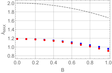
Figure 12: Largest Lyapunov exponent computed at the unstable fixed point $(0,0,0,0)$ as a function of $B$ for $r_{0}=1.1$. The symbols are as in Fig. 11.

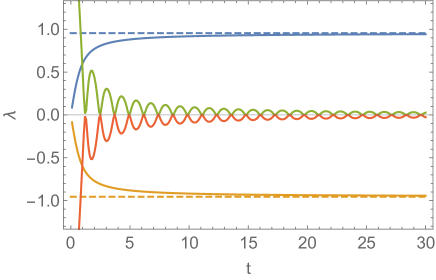
Figure 13: Convergency plot of the Lyapunov exponents for $r_{0}=1.1$ and $B=1$ computed at the unstable fixed point $(0,0,0,0)$. The horizontal lines correspond to the analytical values of the nonvanishing Lyapunov exponents $\sqrt{-\omega_{0}^{2}}$ (top dashed blue line) and $-\sqrt{-\omega_{0}^{2}}$ (bottom dashed orange line).

7 Conclusions

Our investigation of a suspended string in a gravitational background with a black hole, the holographic dual of the heavy quark-antiquark system in a thermal environment, confirms the MSS bounds (1) also in the case of a uniform and constant magnetic field. The system becomes less chaotic increasing $B$. The anisotropy effect in two different orientations of the string is found. This conclusion is analogous to the one obtained for different geometries, namely AdS-RN [24], as well as studying the charged particle motion in such a kind of background [35]. Chaos has been observed in the Poincaré plots, characterized by scattered points in the region close to the black-hole horizon, and quantitatively described computing the Lyapunov exponents, finding that the largest one verifies the MSS bound. The stabilization effect of the magnetic field is stronger for the string endpoints lying on a line parallel to the field, keeping the black-hole horizon and the position of the tip of the string fixed. The largest Lyapunov exponents are below the MSS bound also at the fixed unstable point of the potential describing the perturbed string approaching the horizon.

Acknowledgements. We thank F. De Fazio and S. Nicotri for discussions. This study has been carried out within the INFN project (Iniziativa Specifica) QFT-HEP.

References

- [1] J. Maldacena, S. H. Shenker, and D. Stanford, A bound on chaos, JHEP 08 (2016) 106, [arXiv:1503.01409].
- [2] Y. Sekino and L. Susskind, Fast Scramblers, JHEP 10 (2008) 065, [arXiv:0808.2096].
- [3] L. Susskind, Addendum to Fast Scramblers, arXiv:1101.6048.
- [4] S. H. Shenker and D. Stanford, Black holes and the butterfly effect, JHEP 03 (2014) 067, [arXiv:1306.0622].
- [5] S. H. Shenker and D. Stanford, Stringy effects in scrambling, JHEP 05 (2015) 132, [arXiv:1412.6087].
- [6] A. Kitaev, Hidden correlations in the Hawking radiation and thermal noise, Breakthrough Prize Fundamental Physics Symposium, 11/10/2014, KITP seminar (2014).
- [7] J. Polchinski, Chaos in the black hole S-matrix, arXiv:1505.08108.
- [8] L. Susskind, Why do Things Fall?, arXiv:1802.01198.
- [9] A. R. Brown, H. Gharibyan, A. Streicher, L. Susskind, L. Thorlacius, and Y. Zhao, Falling Toward Charged Black Holes, Phys. Rev. D 98 (2018), no. 12 126016, [arXiv:1804.04156].
- [10] J. M. Maldacena, Wilson loops in large N field theories, Phys. Rev. Lett. 80 (1998) 4859–4862, [hep-th/9803002].
- [11] E. Witten, Anti-de Sitter space and holography, Adv. Theor. Math. Phys. 2 (1998) 253, [hep-th/9802150].
- [12] S. Gubser, I. R. Klebanov, and A. M. Polyakov, Gauge theory correlators from noncritical string theory, Phys. Lett. B 428 (1998) 105–114, [hep-th/9802109].
- [13] J. de Boer, E. Llabrs, J. F. Pedraza, and D. Vegh, Chaotic strings in AdS/CFT, Phys. Rev. Lett. 120 (2018), no. 20 201604, [arXiv:1709.01052].
- [14] S. Dalui, B. R. Majhi, and P. Mishra, Presence of horizon makes particle motion chaotic, Phys. Lett. B 788 (2019) 486–493, [arXiv:1803.06527].
- [15] S. Dalui and B. R. Majhi, Near horizon local instability and quantum thermality, Phys. Rev. D 102 (2020), no. 12 124047, [arXiv:2007.14312].
- [16] D. S. Ageev, Butterflies dragging the jets: on the chaotic nature of holographic QCD, arXiv:2105.04589.
- [17] S. D. Avramis, K. Sfetsos, and K. Siampos, Stability of strings dual to flux tubes between static quarks in N = 4 SYM, Nucl. Phys. B 769 (2007) 44–78, [hep-th/0612139].
- [18] R. E. Arias and G. A. Silva, Wilson loops stability in the gauge/string correspondence, JHEP 01 (2010) 023, [arXiv:0911.0662].
- [19] C. Nunez, M. Piai, and A. Rago, Wilson Loops in string duals of Walking and Flavored Systems, Phys. Rev. D 81 (2010) 086001, [arXiv:0909.0748].
- [20] L. Bellantuono, P. Colangelo, F. De Fazio, F. Giannuzzi, and S. Nicotri, Quarkonium dissociation in a far-from-equilibrium holographic setup, Phys. Rev. D 96 (2017), no. 3 034031, [arXiv:1706.04809].
- [21] K. Hashimoto, K. Murata, and N. Tanahashi, Chaos of Wilson Loop from String Motion near Black Hole Horizon, Phys. Rev. D 98 (2018), no. 8 086007, [arXiv:1803.06756].
- [22] T. Ishii, K. Murata, and K. Yoshida, Fate of chaotic strings in a confining geometry, Phys. Rev. D 95 (2017), no. 6 066019, [arXiv:1610.05833].
- [23] T. Akutagawa, K. Hashimoto, K. Murata, and T. Ota, Chaos of QCD string from holography, Phys. Rev. D 100 (2019), no. 4 046009, [arXiv:1903.04718].
- [24] P. Colangelo, F. De Fazio, and N. Losacco, Chaos in a system at finite temperature and baryon density, Phys. Rev. D 102 (2020), no. 7 074016, [arXiv:2007.06980].
- [25] R. Critelli, R. Rougemont, S. I. Finazzo, and J. Noronha, Polyakov loop and heavy quark entropy in strong magnetic fields from holographic black hole engineering, Phys. Rev. D 94 (2016), no. 12 125019, [arXiv:1606.09484].
- [26] A. Ballon-Bayona, J. P. Shock, and D. Zoakos, Magnetic catalysis and the chiral condensate in holographic QCD, JHEP 10 (2020) 193, [arXiv:2005.00500].
- [27] I. Y. Aref’eva, K. Rannu, and P. Slepov, Holographic model for heavy quarks in anisotropic hot dense QGP with external magnetic field, JHEP 07 (2021) 161, [arXiv:2011.07023].
- [28] I. Y. Aref’eva, K. Rannu, and P. Slepov, Energy Loss in Holographic Anisotropic Model for Heavy Quarks in External Magnetic Field, arXiv:2012.05758.
- [29] I. Y. Aref’eva, K. Rannu, and P. S. Slepov, Anisotropic solutions for a holographic heavy-quark model with an external magnetic field, Teor. Mat. Fiz. 207 (2021), no. 1 44–57.
- [30] E. D’Hoker and P. Kraus, Magnetic Brane Solutions in AdS, JHEP 10 (2009) 088, [arXiv:0908.3875].
- [31] E. D’Hoker and P. Kraus, Charged Magnetic Brane Solutions in AdS (5) and the fate of the third law of thermodynamics, JHEP 03 (2010) 095, [arXiv:0911.4518].
- [32] D. Li, M. Huang, Y. Yang, and P.-H. Yuan, Inverse Magnetic Catalysis in the Soft-Wall Model of AdS/QCD, JHEP 02 (2017) 030, [arXiv:1610.04618].
- [33] N. R. F. Braga, Y. F. Ferreira, and L. F. Ferreira, Configuration entropy and stability of bottomonium radial excitations in a plasma with magnetic fields, arXiv:2110.04560.
- [34] M. Sandri, Numerical calculation of lyapunov exponents, Mathematica Journal 6 (1996), no. 3 78–84.
- [35] D. S. Ageev and I. Y. Aref’eva, When things stop falling, chaos is suppressed, JHEP 01 (2019) 100, [arXiv:1806.05574].