Exploring smoking-gun signals
of the Schwinger mechanism in QCD

Abstract

In QCD, the Schwinger mechanism endows the gluons with an effective mass through the dynamical formation of massless bound-state poles that are longitudinally coupled. The presence of these poles affects profoundly the infrared properties of the interaction vertices, inducing crucial modifications to their fundamental Ward identities. Within this general framework, we present a detailed derivation of the non-Abelian Ward identity obeyed by the pole-free part of the three-gluon vertex in the soft-gluon limit, and determine the smoking-gun displacement that the onset of the Schwinger mechanism produces to the standard result. Quite importantly, the quantity that describes this distinctive feature coincides formally with the bound-state wave function that controls the massless pole formation. Consequently, this signal may be computed in two independent ways: by solving an approximate version of the pertinent Bethe-Salpeter integral equation, or by appropriately combining the elements that enter in the aforementioned Ward identity. For the implementation of both methods we employ two- and three-point correlation functions obtained from recent lattice simulations, and a partial derivative of the ghost-gluon kernel, which is computed from the corresponding Schwinger-Dyson equation. Our analysis reveals an excellent coincidence between the results obtained through either method, providing a highly nontrivial self-consistency check for the entire approach. When compared to the null hypothesis, where the Schwinger mechanism is assumed to be inactive, the statistical significance of the resulting signal is estimated to be three standard deviations.

I Introduction

The systematic study of the fundamental $n$-point correlation (Green’s) functions, such as propagators and vertices, forms an essential element in the ongoing quest for unraveling the nonperturbative properties and underlying dynamical mechanisms of QCD Marciano and Pagels (1978). In recent years, this challenging problem has been tackled by means of approaches formulated in the continuum, such as the Schwinger-Dyson equations (SDEs) Roberts and Williams (1994); Alkofer and von Smekal (2001); Fischer (2006); Roberts (2008); Binosi and Papavassiliou (2009); Binosi et al. (2015); Cloet and Roberts (2014); Aguilar et al. (2016a); Binosi et al. (2016, 2017); Huber (2020) or the functional renormalization group Pawlowski et al. (2004); Pawlowski (2007); Cyrol et al. (2018a); Corell et al. (2018); Blaizot et al. (2021), in conjunction with numerous gauge-fixed lattice simulations Cucchieri and Mendes (2007, 2008, 2010); Bogolubsky et al. (2007, 2009); Oliveira and Silva (2009); Oliveira and Bicudo (2011); Maas (2013); Boucaud et al. (2012); Oliveira and Silva (2012). This intense activity has delivered new insights on the nature and phenomenology of the strong interactions and has broadened our basic understanding of non-Abelian gauge theories Maris and Roberts (1997, 2003); Braun et al. (2010); Eichmann et al. (2009); Cloet et al. (2009); Boucaud et al. (2008); Eichmann et al. (2010); Fister and Pawlowski (2013); Meyer and Swanson (2015); Eichmann et al. (2016); Sanchis-Alepuz et al. (2018); Alkofer et al. (2019); Gao et al. (2018); Souza et al. (2020); Xu et al. (2019); Aguilar et al. (2019a); Huber et al. (2020); Roberts and Schmidt (2020); Roberts (2020); Horak et al. (2021); Roberts (2021).

In this context, the characteristic feature of infrared saturation displayed by the gluon propagator has attracted particular attention, being often linked with the emergence of a mass gap in the gauge sector of QCD Smit (1974); Cornwall (1982); Bernard (1982, 1983); Donoghue (1984); Mandula and Ogilvie (1987); Cornwall and Papavassiliou (1989); Wilson et al. (1994); Philipsen (2002); Aguilar et al. (2003); Aguilar and Natale (2004); Aguilar and Papavassiliou (2006); Aguilar et al. (2008); Fischer et al. (2009); Tissier and Wschebor (2010); Binosi et al. (2012); Serreau and Tissier (2012); Peláez et al. (2014); Aguilar et al. (2016b). This property has been explored both in large-volume simulations Cucchieri and Mendes (2007, 2008); Bogolubsky et al. (2007, 2009); Oliveira and Silva (2009); Oliveira and Bicudo (2011); Cucchieri and Mendes (2010), and in various functional approaches Aguilar et al. (2008); Fischer et al. (2009); Binosi et al. (2012); Serreau and Tissier (2012); Tissier and Wschebor (2010); Aguilar et al. (2016b); Peláez et al. (2014); Dudal et al. (2008); Rodríguez-Quintero (2011); Pennington and Wilson (2011); Meyers and Swanson (2014); Siringo (2016); Cyrol et al. (2018b), and is rather general, manifesting itself in the Landau gauge, away from it Cucchieri et al. (2009, 2010); Bicudo et al. (2015); Epple et al. (2008); Campagnari and Reinhardt (2010); Aguilar et al. (2017); Glazek et al. (2017), and in the presence of dynamical quarks Bowman et al. (2007); Kamleh et al. (2007); Ayala et al. (2012); Aguilar et al. (2013, 2020a). In general terms, the scalar form factor, $\Delta(q^{2})$, of the gluon propagator reaches a finite nonvanishing value in the deep infrared, and the gluon mass, $m$, is identified as $\Delta^{-1}(0)=m^{2}$.

One of the nonperturbative mechanisms put forth in order to explain this special behavior of the gluon propagator is based on a non-Abelian extension of the well-known Schwinger mechanism Schwinger (1962a, b). According to the fundamental observation underlying this mechanism, if the self-energy develops a pole at zero momentum transfer ($q^{2}=0$), then the corresponding vector meson (gluon) acquires a mass, even if the gauge symmetry forbids a mass term at the level of the fundamental Lagrangian Schwinger (1962a, b); Jackiw and Johnson (1973); Eichten and Feinberg (1974).

The precise implementation of this idea at the level of the SDE describing the momentum evolution of $\Delta(q^{2})$ requires the inclusion of longitudinally coupled massless poles at the level of the fundamental interaction vertices of the theory Aguilar et al. (2012); Ibañez and Papavassiliou (2013); Binosi and Papavassiliou (2018); Aguilar et al. (2018); Binosi and Papavassiliou (2018); Eichmann et al. (2021). These poles are produced as massless bound state excitations, whose formation is governed by a special set of Bethe-Salpeter equations (BSEs) Aguilar et al. (2012); Ibañez and Papavassiliou (2013); Aguilar et al. (2018); Binosi and Papavassiliou (2018). In addition, their presence is crucial for maintaining intact the form of the Slavnov-Taylor identities (STIs) Taylor (1971); Slavnov (1972) satisfied by the corresponding vertices. Since the fully dressed vertices enter in the diagrammatic expansion of the gluon SDE, their massless poles end up triggering the Schwinger mechanism, enabling a completely dynamical generation of an effective gluon mass Aguilar et al. (2012); Binosi et al. (2012); Ibañez and Papavassiliou (2013); Aguilar et al. (2018); Binosi and Papavassiliou (2018).

It is clearly important to further scrutinize the dynamical picture described above, and identify certain characteristic properties that would corroborate its validity and discriminate it from alternative dynamical scenarios. In the present work we explore a distinctive signal of the non-Abelian Schwinger mechanism, which is intimately connected with the three-gluon vertex, and has the advantage of being reliably calculable by means of well-established inputs, such as two- and three-point correlation functions obtained from large-volume lattice simulations.

The pivotal ideas underlying this study may be summarized as follows. The massless poles are longitudinally coupled, and therefore drop out from “on-shell” observables Jackiw and Johnson (1973); Cornwall and Norton (1973); Eichten and Feinberg (1974); Poggio et al. (1975); Smit (1974), or from the transversely projected vertices employed in lattice simulations  Cucchieri et al. (2006, 2008); Athenodorou et al. (2016); Duarte et al. (2016); Boucaud et al. (2018); Aguilar et al. (2020a), where only the pole-free part of the corresponding vertex survives. Nonetheless, the imprint of the poles is invariably encoded into the pole-free part, as may be seen by considering the Ward identity (WI) that this latter part satisfies, namely the limit of the STI as the gluon momentum in the channel of the pole is taken to zero.

Since the poles contribute nontrivially to the STIs, the corresponding WI involves the standard building blocks (e.g., propagators) and a residual contribution with a nontrivial momentum dependence, which is directly related to the Schwinger mechanism. As a result, in that kinematic limit, the relevant form factor of the pole-free part of the vertex is displaced with respect to the case where the Schwinger mechanism is absent.

The above considerations become particularly relevant in the case of the three-gluon vertex, because the form factor of its pole-free part has been evaluated rather accurately in recent lattice simulations Boucaud et al. (2003, 2004); Aguilar et al. (2021a). As a result, the displacement originating from the onset of the Schwinger mechanism, to be denoted by ${\mathbb{C}}(r^{2})$, may be calculated by appropriately combining this form factor with all other constituents that enter into the WI of the three-gluon vertex; all of them are available from lattice simulations, with the exception of a particular partial derivative, denoted by ${\cal W}(r^{2})$, related to the ghost-gluon kernel that appears in the STI Aguilar et al. (2020b, 2021b).

The importance of the calculation put forth above becomes particularly transparent when an additional theoretical ingredient is taken into account. Specifically, as will become clear in the main body of the article, ${\mathbb{C}}(r^{2})$ coincides exactly with the wave function amplitude of the massless bound state poles associated with the three-gluon vertex Aguilar et al. (2012); Ibañez and Papavassiliou (2013); Aguilar et al. (2018); Binosi and Papavassiliou (2018). Thus, the form of ${\mathbb{C}}(r^{2})$ is determined from an entirely different procedure, namely as the solution of the BSE mentioned earlier. This solution, in turn, serves as a benchmark of our analysis, in the sense that signals emerging from the WI treatment are expected to be qualitatively compatible with the ${\mathbb{C}}(r^{2})$ obtained from the BSE Aguilar et al. (2012); Ibañez and Papavassiliou (2013); Aguilar et al. (2018); Binosi and Papavassiliou (2018).

Our numerical analysis reveals that the ${\mathbb{C}}(r^{2})$ constructed by putting together all the ingredients of the WI deviates markedly from zero, showing an impressive resemblance to the results obtained from the corresponding BSE. On the average, the signal obtained is $3.1\sigma$ away from the null hypothesis value, ${\mathbb{C}}(r^{2})=0$, which corresponds to the absence of the Schwinger mechanism. Moreover, for momenta $r\geq 2$ GeV the deviation of the signal from ${\mathbb{C}}(r^{2})=0$ exceeds the $5\sigma$, owing to a characteristic peak of ${\mathbb{C}}(r^{2})$ in the vicinity of $2$ GeV, and to the fact that the error bars assigned to the lattice points get reduced as one moves away from the deep infrared region.

Let us finally mention that the principal uncertainty associated with the WI determination originates from the computation of the function ${\cal W}(r^{2})$, which is not available from lattice simulations, and has been approximated by a truncated version of the SDE of the ghost-gluon kernel. As was explained in Aguilar et al. (2021b), the simulation of this function on the lattice is theoretically conceivable, but practically rather cumbersome.

The article is organized as follows. In Sec. II we explain in an Abelian context how the presence of longitudinally coupled massless poles modifies the form of the WI satisfied by the pole-free part of a vertex. In Sec. III we derive the corresponding WI for the pole-free part of the three-gluon vertex, introducing the displacement function ${\mathbb{C}}(r^{2})$. Then, in Sec. IV we express ${\mathbb{C}}(r^{2})$ in terms of the three-gluon form factor, the gluon propagator and its derivative, the ghost dressing function, and the function ${\cal W}(r^{2})$. Next, in Sec. V we present the BSE determination of ${\mathbb{C}}(r^{2})$. In Sec. VI we use lattice inputs for the components of the WI in order to determine the form of ${\mathbb{C}}(r^{2})$, and compare it to the corresponding result obtained from the BSE. Finally, in Sec. VII we present our discussion and conclusions. In addition, certain topics have been relegated to three Appendices: Appendix A contains technical details of the BSE treatment, in Appendix B we discuss the SDE-based determination of ${\cal W}(r^{2})$, while in Appendix C we collect the fits employed in our numerical analysis.

II Ward identities in the presence of massless poles

In this section we focus on the modifications induced to the form of the WIs when the vertices involved contain longitudinally coupled massless poles, which is one of the trademarks of the Schwinger mechanism at the level of the vertices.

In general, the derivation of the WI from the corresponding Takahashi identity, or, in general, from a given STI, involves a Taylor expansion around the contracting momentum Aguilar et al. (2016b). In the case of a function of a single variable, $f((p+q)^{2})$, such as a propagator, the Taylor expansion proceeds through the elementary formula ($q\to 0$)

$$f((p+q)^{2}) = f(p^{2})+q^{\alpha}\,\frac{\partial f(p^{2})}{\partial p^{\alpha}}+{\cal O}(q^{2})$$ (1)

$$= f(p^{2})+2(q\cdot p)\,\frac{\partial f(p^{2})}{\partial p^{2}}+{\cal O}(q^{2})\,.$$

For a function $f(q,r,p)$, with $q+r+p=0$, such as a three-particle vertex or kernel, the Taylor expansion around $q=0$ (and $p=-r$) gives

$$f(q,r,p)=f(0,r,-r)+q^{\alpha}\left[\frac{\partial f(q,r,p)}{\partial q^{\alpha}}\right]_{q=0}+{\cal O}(q^{2})\,.$$ (2)

Note that if the $f(q,r,p)=-f(q,p,r)$, as happens in the case of the term associated with the massless pole in the $q$ channel (see below), then $f(0,r,-r)=0$.

In order to fix the ideas, we employ a vertex with reduced tensorial structure, which obeys an Abelian STI. In particular, we consider one of the typical vertices of the background field method (BFM) DeWitt (1967); Honerkamp (1972); ’t Hooft (1971); Kallosh (1974); Kluberg-Stern and Zuber (1975); Abbott (1981); Shore (1981); Abbott et al. (1983), namely the $B(q){\bar{c}}(r)c(p)$ vertex, where $B$ denotes the background gluon and ${\bar{c}}$ ($c$) the anti-ghost (ghost) fields. Due to the residual invariance of the action under background gauge transformations, this vertex satisfies an Abelian STI that relates it to the inverse ghost propagator. Specifically, suppressing the gauge coupling $g$ and the color factor $f^{abc}$, and denoting the remainder of the vertex by $\widetilde{\Gamma}_{\alpha}(q,r,p)$, we have Aguilar and Papavassiliou (2006); Binosi and Papavassiliou (2009)

$$q^{\alpha}\widetilde{\Gamma}_{\alpha}(q,r,p)={D}^{-1}(p^{2})-{D}^{-1}(r^{2})\,,$$ (3)

where the ghost propagator is given by $D^{ab}(q^{2})=i\delta^{ab}D(q^{2})$. Note that, at tree level, $\widetilde{\Gamma}_{\!0}^{\alpha}(q,r,p)=(r-p)^{\alpha}$.

At this point we will assume that the Schwinger mechanism is inactive, such that the form factors comprising $\widetilde{\Gamma}_{\alpha}(q,r,p)$ do not contain poles. In that case, one may carry out the Taylor expansion of both sides of Eq. (3) according to Eqs. (1) and (2). Specifically, the left hand-side (l.h.s) of Eq. (3) yields

$$[{\rm l.h.s}]=q^{\alpha}\widetilde{\Gamma}_{\alpha}(0,r,-r)\,+{\cal O}(q^{2})\,,$$ (4)

while the right hand-side (r.h.s) is simply given by

$$[{\rm r.h.s}]=q^{\alpha}\frac{\partial{D}^{-1}(r^{2})}{\partial r^{\alpha}}\,+{\cal O}(q^{2})\,.$$ (5)

Then, equating the coefficients of the terms linear in $q^{\alpha}$ on both sides, one obtains the simple, QED-like relation Aguilar et al. (2016b)

$$\widetilde{\Gamma}_{\alpha}(0,r,-r)=\,\frac{\partial{D}^{-1}(r^{2})}{\partial r^{\alpha}}\,.$$ (6)

Finally, at the level of the single form factor comprising $\widetilde{\Gamma}_{\alpha}(0,r,-r)$, namely

$$\widetilde{\Gamma}_{\alpha}(0,r,-r)=\widetilde{\cal A}(r^{2})r_{\alpha}\,,$$ (7)

we obtain directly from Eq. (6) Aguilar et al. (2016b)

$$\widetilde{\cal A}(r^{2})=2\frac{\partial{D}^{-1}(r^{2})}{\partial r^{2}}\,.$$ (8)

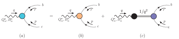
Figure 1: ($a$): Compact diagrammatic representation of the vertices $\widetilde{{\rm{I}}\!\Gamma}_{\alpha}(q,r,p)$ ($B$ gluon) and ${\rm{I}}\!\Gamma_{\alpha}(q,r,p)$ ($Q$ gluon); ($b$) the pole-free parts, $\widetilde{\Gamma}_{\alpha}(q,r,p)$ and $\Gamma_{\alpha}(q,r,p)$; ($c$) the pole parts, ${\widetilde{V}}_{\alpha}(q,r,p)$ and ${V}_{\alpha}(q,r,p)$. The black circle denotes the “transition amplitude”, describing the mixing of the gluon with a massless excitation; its detailed diagrammatic content may be found in Ibañez and Papavassiliou (2013).

Let us now turn the Schwinger mechanism on, and denote the resulting full vertex by $\widetilde{\rm{I}}\!\Gamma_{\alpha}(q,r,p)$. The vertex $\widetilde{\rm{I}}\!\Gamma_{\alpha}(q,r,p)$, diagrammatically represented in Fig. 1, is comprised by two distinct pieces,

$$\widetilde{{\rm{I}}\!\Gamma}_{\alpha}(q,r,p)=\widetilde{\Gamma}_{\alpha}(q,r,p)+{\widetilde{V}}_{\alpha}(q,r,p),$$ (9)

where $\widetilde{\Gamma}_{\alpha}(q,r,p)$ contains all pole-free contributions, while the pole term ${\widetilde{V}}_{\alpha}(q,r,p)$ has the general form Jackiw and Johnson (1973); Cornwall and Norton (1973); Eichten and Feinberg (1974); Poggio et al. (1975); Smit (1974),

$${\widetilde{V}}_{\alpha}(q,r,p)=\frac{q_{\alpha}}{q^{2}}{\widetilde{C}}(q,r,p)\,.$$ (10)

We emphasize that the pole-free terms $\widetilde{\Gamma}_{\alpha}(q,r,p)$ are different when the Schwinger mechanism is turned on or off. In particular, the infrared finiteness of the gluon propagator affects the behavior of all other Green’s function, due to its nontrivial interconnection with them imposed by the corresponding coupled SDEs. A typical qualitative example of the type of modifications that the emergence of a gluonic mass scale induces to one-loop contributions is the conversion of “unprotected” logarithms into “protected” ones, according to $\ln({q^{2}}/{\mu^{2}})\to\ln[(q^{2}+m^{2})/{\mu^{2}}]$ Aguilar et al. (2014); Athenodorou et al. (2016).

Evidently, combining Eqs. (9) and (10) we get

$$q^{\alpha}\widetilde{{\rm{I}}\!\Gamma}_{\alpha}(q,r,p)=q^{\alpha}\widetilde{\Gamma}_{\alpha}(q,r,p)+\widetilde{C}(q,r,p)\,;$$ (11)

thus, the contraction by $q^{\alpha}$ cancels the massless pole in $q^{2}$.

We next assume that the Becchi-Rouet-Stora-Tyutin (BRST) symmetry Becchi et al. (1976); Tyutin (1975) of the theory remains intact as the Schwinger mechanism becomes operational. In particular, the STIs satisfied by the elementary vertices are assumed to retain their standard form, but now being realized through the nontrivial participation of the massless pole terms Eichten and Feinberg (1974); Poggio et al. (1975); Smit (1974); Cornwall (1982); Papavassiliou (1990); Aguilar et al. (2008); Binosi et al. (2012); Aguilar et al. (2016b). For a variety of perspectives related to the BRST symmetry in the presence of a mass gap, see, e.g.,  Alkofer and von Smekal (2001); Fischer et al. (2009); Alkofer and Alkofer (2011); Capri et al. (2015), and references therein.

Accordingly, the full $\widetilde{{\rm{I}}\!\Gamma}_{\alpha}(q,r,p)$ satisfies, as before, precisely Eq. (3), namely

$$q^{\alpha}\widetilde{{\rm{I}}\!\Gamma}_{\alpha}(q,r,p)={D}^{-1}(p^{2})-{D}^{-1}(r^{2})\,,$$ (12)

where $D(q^{2})$ is the ghost propagator in the presence of the Schwinger mechanism. For the same reasons described above for the case of $\widetilde{\Gamma}_{\alpha}(q,r,p)$, $D(q^{2})$ also differs from the corresponding quantity when the Schwinger mechanism is not operational.

Then, using Eq. (11), we obtain for the pole-free part

$$q^{\alpha}\widetilde{\Gamma}_{\alpha}(q,r,p)=\left[D^{-1}(p^{2})-D^{-1}(r^{2})\right]\,-\widetilde{C}(q,r,p)\,.$$ (13)

The WI obeyed by $\widetilde{\Gamma}_{\alpha}(q,r,p)$ may be derived again by means of a Taylor expansion, since, after the contraction by $q^{\alpha}$, all terms appearing in the STI of Eq. (13) contain no poles, as $q\to 0$. In particular,

$$q^{\alpha}\widetilde{\Gamma}_{\alpha}(0,r,-r)=\widetilde{C}(0,r,-r)+q^{\alpha}\left\{\frac{\partial{D}^{-1}(r^{2})}{\partial r^{\alpha}}-\left[\frac{\partial\widetilde{C}(q,r,p)}{\partial q^{\alpha}}\right]_{q=0}\right\}\,+{\cal O}(q^{2})\,.$$ (14)

The comparison between Eqs. (14) and (5) reveals that the only zeroth-order contribution, namely $\widetilde{C}(0,r,-r)$, must vanish,

$$\widetilde{C}(0,r,-r)=0\,.$$ (15)

Note that the result of Eq. (15) may be independently obtained from the property $\widetilde{C}(q,r,p)=-\widetilde{C}(q,p,r)$, which follows directly from the general ghost-antighost symmetry of the $B(q){\bar{c}}(r)c(p)$ vertex.

Then, the matching of the terms linear in $q$ yields the WI

$$\widetilde{\Gamma}_{\alpha}(0,r,-r)=\frac{\partial{D}^{-1}(r^{2})}{\partial r^{\alpha}}-\underbrace{\left[\frac{\partial\widetilde{C}(q,r,p)}{\partial q^{\alpha}}\right]_{q=0}}_{\rm WI\,\,displacement}\,,$$ (16)

which, when compared to that of Eq. (6), is “displaced” by the partial derivative of the form factor associated with the pole term.

In order to determine the displaced analogue of Eq. (8), we set

$$\left[\frac{\partial\widetilde{C}(q,r,p)}{\partial q^{\alpha}}\right]_{q=0}\!\!\!\!\!=2r_{\alpha}\,{\widetilde{\mathcal{C}}}(r^{2})\,,\qquad{\widetilde{\mathcal{C}}}(r^{2}):=\left[\frac{\partial\widetilde{C}(q,r,p)}{\partial p^{2}}\right]_{q=0}\,,$$ (17)

and obtain immediately from Eqs. (7) and (16)

$$\widetilde{\cal A}(r^{2})=2\left[\frac{\partial{D}^{-1}(r^{2})}{\partial r^{2}}-\,{\widetilde{\mathcal{C}}}(r^{2})\right]\,.$$ (18)

Note that the displacement of the WI exemplified above becomes especially relevant within the framework that combines the pinch-technique (PT) Cornwall (1982); Cornwall and Papavassiliou (1989); Pilaftsis (1997); Binosi and Papavassiliou (2009) with the BFM, known as “PT-BFM scheme” Aguilar and Papavassiliou (2006); Binosi and Papavassiliou (2008). In particular, the action of terms such as ${\widetilde{\mathcal{C}}}(r^{2})$ is instrumental for the evasion of a powerful nonperturbative cancellation that operates at the level of the gluon SDE Aguilar and Papavassiliou (2010), which would otherwise enforce the result $\Delta^{-1}(0)=0$. In fact, the contribution of the ghost loop to the nonvanishing $\Delta^{-1}(0)$, to be denoted by $\Delta_{\rm gh}^{-1}(0)$, is given by Aguilar et al. (2016b)

$$\Delta_{\rm gh}^{-1}(0)\sim\int\!\!d^{4}k\,k^{2}D^{2}(k^{2}){\widetilde{\mathcal{C}}}(k^{2})\,.$$ (19)

Let us finally point out that the displacement associated with the conventional ghost-gluon vertex ${\rm{I}}\!\Gamma_{\alpha}(q,r,p)$ [see Fig. 1], to be denoted by ${\mathcal{C}}(r^{2})$ [see Eq. (65)], is related to ${\widetilde{\mathcal{C}}}(r^{2})$ by the simple relation

$${\mathcal{C}}(r^{2})=F(0)\,{\widetilde{\mathcal{C}}}(r^{2})\,.$$ (20)

The demonstration of Eq. (20) relies on the “background-quantum identity” that relates $\widetilde{\rm{I}}\!\Gamma_{\alpha}(q,r,p)$ and ${\rm{I}}\!\Gamma_{\alpha}(q,r,p)$ Binosi and Papavassiliou (2002, 2009); details will be presented elsewhere.

III Three-gluon vertex and its Ward identity displacement

In this section we consider the case of the three-gluon vertex in the conventional Landau gauge. If this vertex develops longitudinally coupled massless poles, its pole-free part satisfies a displaced WI, whose derivation is the focal point of this section.

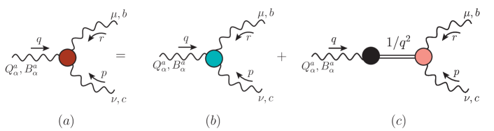
Figure 2: ($a$): Compact diagrammatic representation of the vertices $\widetilde{{\rm{I}}\!\Gamma}_{\alpha\mu\nu}(q,r,p)$ ($B$ gluon) and ${\rm{I}}\!\Gamma_{\alpha\mu\nu}(q,r,p)$ ($Q$ gluon); ($b$) the pole-free parts, ${\widetilde{\Gamma}}_{\alpha\mu\nu}(q,r,p)$ and $\Gamma_{\alpha\mu\nu}(q,r,p)$; ($c$) the pole parts, ${\widetilde{V}}_{\alpha\mu\nu}(q,r,p)$ and ${V}_{\alpha\mu\nu}(q,r,p)$.

Before commencing, we introduce the gluon propagator, $\Delta^{ab}_{\mu\nu}(q)=-i\delta^{ab}\Delta_{\mu\nu}(q)$; in the Landau gauge that we employ in this work, it is given by the completely transverse form

$$\Delta_{\mu\nu}(q)=\Delta(q^{2}){P}_{\mu\nu}(q)\,,\qquad{P}_{\mu\nu}(q):=g_{\mu\nu}-q_{\mu}q_{\nu}/{q^{2}}\,.$$ (21)

In addition, we will use the ghost dressing function, $F(q^{2})$, related to the ghost propagator by $F(q^{2})=q^{2}D(q^{2})$. Furthermore, we define the two tensorial structures

$${P}_{\mu^{\prime}}^{\mu}(r){P}_{\nu^{\prime}}^{\nu}(-r):={\cal T}_{\mu^{\prime}\nu^{\prime}}^{\mu\nu}(r)\,,\qquad\lambda_{\mu\nu\alpha}(r):=2r_{\alpha}P_{\mu\nu}(r)\,,$$ (22)

and the tree-level three-gluon vertex, $\Gamma_{\!0}^{\alpha\mu\nu}(q,r,p)$, as

$$\Gamma_{\!0}^{\alpha\mu\nu}(q,r,p)=(q-r)^{\nu}g^{\alpha\mu}+(r-p)^{\alpha}g^{\mu\nu}+(p-q)^{\mu}g^{\nu\alpha}\,,$$ (23)

where the gauge coupling $g$ and the color factor $f^{abc}$ were suppressed.

In order for the Schwinger mechanism to be activated, the full three-gluon vertex, to be denoted by ${\rm{I}}\!\Gamma^{abc}_{\alpha\mu\nu}(q,r,p)=gf^{abc}{\rm{I}}\!\Gamma_{\alpha\mu\nu}(q,r,p)$, is written as (see Fig. 2)

$${\rm{I}}\!\Gamma_{\alpha\mu\nu}(q,r,p)=\Gamma_{\alpha\mu\nu}(q,r,p)+V_{\alpha\mu\nu}(q,r,p)\,,$$ (24)

where $\Gamma_{\alpha\mu\nu}(q,r,p)$ is the pole-free component, while $V_{\alpha\mu\nu}(q,r,p)$ contains longitudinally coupled poles, i.e.,   it assumes the general form

$$V_{\alpha\mu\nu}(q,r,p)=\left(\frac{q_{\alpha}}{q^{2}}\right)C_{\mu\nu}(q,r,p)+\left(\frac{r_{\mu}}{r^{2}}\right)A_{\alpha\nu}(q,r,p)+\left(\frac{p_{\nu}}{p^{2}}\right)B_{\alpha\mu}(q,r,p)\,.$$ (25)

For the particular kinematic limit that we will eventually consider in the present work ($q\to 0$), we only require the tensorial decomposition of the term $C_{\mu\nu}(q,r,p)$ in Eq. (25), given by

$$C_{\mu\nu}(q,r,p)=C_{1}\,g_{\mu\nu}+C_{2}\,r_{\mu}r_{\nu}+C_{3}\,p_{\mu}p_{\nu}+C_{4}\,r_{\mu}p_{\nu}+C_{5}\,p_{\mu}r_{\nu}\,,$$ (26)

where $C_{i}:=C_{i}(q,r,p)$.

Due to its special form given by Eq. (25), $V_{\alpha\mu\nu}(q,r,p)$ satisfies the crucial condition

$${P}_{\alpha^{\prime}}^{\alpha}(q){P}_{\mu^{\prime}}^{\mu}(r){P}_{\nu^{\prime}}^{\nu}(p)V_{\alpha\mu\nu}(q,r,p)=0\,,$$ (27)

and, consequently, it drops out from the typical lattice observables involving the transversely projected three-gluon vertex [see Eqs. (50) and (74)].

The full vertex ${\rm{I}}\!\Gamma_{\alpha\mu\nu}(q,r,p)$ satisfies the STI

$$q^{\alpha}{\rm{I}}\!\Gamma_{\alpha\mu\nu}(q,r,p)=F(q^{2})\left[\Delta^{-1}(p^{2})P_{\nu}^{\sigma}(p)H_{\sigma\mu}(p,q,r)-\Delta^{-1}(r^{2})P_{\mu}^{\sigma}(r)H_{\sigma\nu}(r,q,p)\right]\,;$$ (28)

analogous expressions are obtained when contracting by $r^{\mu}$ or $p^{\nu}$. Note that the ghost-gluon kernel, $H^{abc}_{\nu\mu}(q,p,r)=-gf^{abc}H_{\nu\mu}(q,p,r)$, defined in Fig. 10, enters in the STI nontrivially; for the nonperturbative structure of its relevant form factors, see Aguilar et al. (2019b). In addition, we point out that the $H_{\sigma\mu}(p,q,r)$ and $H_{\sigma\nu}(r,q,p)$ also contain massless poles in the $r_{\mu}$ and $p_{\nu}$ channels, respectively, which are completely eliminated by the transverse projections in Eq. (32).

It is clear from Eqs. (24) and (26) that

$${P}_{\mu^{\prime}}^{\mu}(r){P}_{\nu^{\prime}}^{\nu}(p)\left[q^{\alpha}{\rm{I}}\!\Gamma_{\alpha\mu\nu}(q,r,p)\right]={P}_{\mu^{\prime}}^{\mu}(r){P}_{\nu^{\prime}}^{\nu}(p)[q^{\alpha}\Gamma_{\alpha\mu\nu}(q,r,p)+C_{\mu\nu}(q,r,p)]\,,$$ (29)

while, from the STI of Eq. (28)

$${P}_{\mu^{\prime}}^{\mu}(r){P}_{\nu^{\prime}}^{\nu}(p)\left[q^{\alpha}{\rm{I}}\!\Gamma_{\alpha\mu\nu}(q,r,p)\right]={P}_{\mu^{\prime}}^{\mu}(r){P}_{\nu^{\prime}}^{\nu}(p)\,F(q^{2})\,{R}_{\nu\mu}(p,q,r)\,,$$ (30)

where

$${R}_{\nu\mu}(p,q,r):=\Delta^{-1}(p^{2})H_{\nu\mu}(p,q,r)-\Delta^{-1}(r^{2})H_{\mu\nu}(r,q,p)\,.$$ (31)

Then, equating the right-hand sides of Eqs. (29) and (30) we obtain

$$q^{\alpha}\left[{P}_{\mu^{\prime}}^{\mu}(r){P}_{\nu^{\prime}}^{\nu}(p)\Gamma_{\alpha\mu\nu}(q,r,p)\right]={P}_{\mu^{\prime}}^{\mu}(r){P}_{\nu^{\prime}}^{\nu}(p)\left[\,F(q^{2})\,{R}_{\nu\mu}(p,q,r)-C_{\mu\nu}(q,r,p)\right]\,.$$ (32)

Due to the presence of the projectors ${P}_{\mu^{\prime}}^{\mu}(r){P}_{\nu^{\prime}}^{\nu}(p)$, it is clear from Eq. (26) that only the terms $C_{1}g_{\mu\nu}$ and $C_{5}\,p_{\mu}r_{\nu}$ contribute to $C_{\mu\nu}(q,r,p)$. Note, however, that since ${P}_{\mu^{\prime}}^{\mu}(r){P}_{\nu^{\prime}}^{\nu}(p)C_{5}\,p_{\mu}r_{\nu}={P}_{\mu^{\prime}}^{\mu}(r){P}_{\nu^{\prime}}^{\nu}(p)C_{5}\,q_{\mu}q_{\nu}$, this term is subleading, i.e., of order ${\cal O}(q^{2})$, when the limit $q\to 0$ is taken.

We next proceed with the implementation of the limit $q\to 0$. In particular, as was done in the previous section, we carry out the Taylor expansion of both sides of Eq. (32) around $q=0$, and collect terms linear in $q$.

The computation of the l.h.s. of Eq. (32) is immediate: using Eq. (22), we have

$$[{\rm l.h.s}]=q^{\alpha}{\cal T}_{\mu^{\prime}\nu^{\prime}}^{\mu\nu}(r)\Gamma_{\alpha\mu\nu}(0,r,-r)+{\cal O}(q^{2})\,.$$ (33)

The computation of the r.h.s. of Eq. (32) is considerably more complicated. We start by noticing that, to lowest order in $q$, only the term $C_{1}(q,r,p)g_{\mu\nu}$ survives. In addition, since it is clear from Eq. (31) that ${R}_{\nu\mu}(-r,0,r)=0$, the vanishing of the zeroth order contribution imposes the condition

$$C_{1}(0,r,-r)=0\,,$$ (34)

in exact analogy to Eq. (15).

Thus, the r.h.s. of Eq. (32) becomes

$$[{\rm r.h.s}]=q^{\alpha}\,{\cal T}_{\mu^{\prime}\nu^{\prime}}^{\mu\nu}(r)F(0)\left[\frac{\partial R_{\nu\mu}(p,q,r)}{\partial q^{\alpha}}\right]_{\!q=0}\!\!\!\!\!-q^{\alpha}\,{P}_{\mu^{\prime}\nu^{\prime}}(r)\left[\frac{\partial C_{1}(q,r,p)}{\partial q^{\alpha}}\right]_{\!q=0}\!\!\!\!\!+{\cal O}(q^{2})\,.$$ (35)

In order to compute the first partial derivative in Eq. (35), we exploit the fact that, in the Landau gauge, the ghost-gluon kernel may be cast in the form Ibañez and Papavassiliou (2013); Aguilar et al. (2020b)

$$H_{\nu\mu}(p,q,r)={\widetilde{Z}}_{1}g_{\nu\mu}+q^{\rho}K_{\nu\mu\rho}(p,q,r)\,,\qquad H_{\mu\nu}(r,q,p)={\widetilde{Z}}_{1}g_{\mu\nu}+q^{\rho}K_{\mu\nu\rho}(r,q,p)\,,$$ (36)

where the kernels $K$ do not contain poles as $q\to 0$. Moreover, ${\widetilde{Z}}_{1}$ is the finite constant renormalizing $H_{\nu\mu}(p,q,r)$ in the “asymmetric” momentum subtraction (MOM) scheme, employed in the lattice simulation of Athenodorou et al. (2016); Aguilar et al. (2020a); its numerical value, estimated in Aguilar et al. (2021c), is ${\widetilde{Z}}_{1}\approx 0.95$.

Then, to lowest order in $q$,

$$\left[\frac{\partial H_{\nu\mu}(p,q,r)}{\partial q^{\alpha}}\right]_{q=0}\!\!\!\!\!\!=K_{\nu\mu\alpha}(-r,0,r)\,,\qquad\left[\frac{\partial H_{\mu\nu}(r,q,p)}{\partial q^{\alpha}}\right]_{q=0}\!\!\!\!\!\!=K_{\mu\nu\alpha}(r,0,-r)\,.$$ (37)

Consider next the tensor decomposition of $K_{\mu\nu\alpha}(r,0,-r)$ Aguilar et al. (2020b),

$$K_{\mu\nu\alpha}(r,0,-r)={K}(r^{2})g_{\mu\nu}r_{\alpha}+\cdots\,,$$ (38)

where the ellipses denote terms proportional to $g_{\nu\alpha}r_{\mu}$, $g_{\mu\alpha}r_{\nu}$, and $r_{\alpha}r_{\mu}r_{\nu}$, which get annihilated by contraction with ${\cal T}_{\mu^{\prime}\nu^{\prime}}^{\mu\nu}(r)$. Clearly, ${\cal T}_{\mu^{\prime}\nu^{\prime}}^{\mu\nu}(r)K_{\nu\mu\alpha}(-r,0,r)=-{\cal T}_{\mu^{\prime}\nu^{\prime}}^{\mu\nu}(r)K_{\mu\nu\alpha}(r,0,-r)$.

Then, it is straightforward to demonstrate that

$${\cal T}_{\mu^{\prime}\nu^{\prime}}^{\mu\nu}(r)\left[\frac{\partial{R}_{\nu\mu}(p,q,r)}{\partial q^{\alpha}}\right]_{\!q=0}\!\!\!\!\!\!=\lambda_{\mu^{\prime}\nu^{\prime}\alpha}(r)\left\{\widetilde{Z}_{1}[\Delta^{-1}(r^{2})]^{\prime}-{K}(r^{2})\Delta^{-1}(r^{2})\right\}\,,$$ (39)

where the “prime” denotes differentiation with respect to $r^{2}$.

As for the second partial derivative in Eq. (35), applying the chain rule we have

$$\left[\frac{\partial C_{1}(q,r,p)}{\partial q^{\alpha}}\right]_{q=0}\!\!\!\!\!\!=2r_{\alpha}{\mathbb{C}}(r^{2})\,,\qquad{\mathbb{C}}(r^{2}):=\left[\frac{\partial C_{1}(q,r,p)}{\partial p^{2}}\right]_{q=0}\,,$$ (40)

such that

$$P_{\mu^{\prime}\nu^{\prime}}(r)\left[\frac{\partial C_{1}(q,r,p)}{\partial q^{\alpha}}\right]_{q=0}\!\!\!\!\!\!=\lambda_{\mu^{\prime}\nu^{\prime}\alpha}(r){\mathbb{C}}(r^{2})\,,$$ (41)

and, therefore, Eq. (35) becomes

$$[{\rm r.h.s}]=q^{\alpha}\lambda_{\mu^{\prime}\nu^{\prime}\alpha}(r)\left[F(0)\left\{\widetilde{Z}_{1}[\Delta^{-1}(r^{2})]^{\prime}-{K}(r^{2})\Delta^{-1}(r^{2})\right\}-{\mathbb{C}}(r^{2})\right]+{\cal O}(q^{2})\,.$$ (42)

The final step is to equate the terms linear in $q$ that appear in Eqs. (33) and (42), to obtain the WI

$${\cal T}_{\mu^{\prime}\nu^{\prime}}^{\mu\nu}(r)\Gamma_{\alpha\mu\nu}(0,r,-r)=\lambda_{\mu^{\prime}\nu^{\prime}\alpha}(r)\left[F(0)\left\{\widetilde{Z}_{1}[\Delta^{-1}(r^{2})]^{\prime}-{K}(r^{2})\Delta^{-1}(r^{2})\right\}-{\mathbb{C}}(r^{2})\right]\,.$$ (43)

Thus, the inclusion of the term $V_{\alpha\mu\nu}(q,r,p)$ in the vertex of Eq. (24) leads ultimately to the displacement of the WI satisfied by the pole-free part $\Gamma_{\alpha\mu\nu}(q,r,p)$, by an amount given by the special function ${\mathbb{C}}(r^{2})$. Evidently, if ${\mathbb{C}}(r^{2})=0$ one recovers the WI in the absence of the Schwinger mechanism.

We end this section with some remarks related to the PT-BFM scheme. Note that if the gauge field carrying the momentum $q$ is a background gluon instead of a quantum one (see Fig. 2), then the corresponding three-gluon vertex, $\widetilde{\Gamma}_{\alpha\mu\nu}(q,r,p)$, satisfies a simplified version of the WI in Eq. (43), where $F\to 1$, $\widetilde{Z}_{1}\to 1$, and ${K}(r^{2})\to 0$, i.e.,

$${\cal T}_{\mu^{\prime}\nu^{\prime}}^{\mu\nu}(r)\widetilde{\Gamma}_{\alpha\mu\nu}(0,r,-r)=\lambda_{\mu^{\prime}\nu^{\prime}\alpha}(r)\left[[\Delta^{-1}(r^{2})]^{\prime}-\widetilde{\mathbb{C}}(r^{2})\right]\,.$$ (44)

As has been demonstrated in Aguilar et al. (2016b), the contribution of the gluon loops to the nonvanishing $\Delta^{-1}(0)$, to be denoted by $\Delta_{\rm gl}^{-1}(0)$, is controlled by $\widetilde{\mathbb{C}}(r^{2})$,

$$\Delta_{\rm gl}^{-1}(0)\sim\int\!\!d^{4}k\,k^{2}\Delta^{2}(k^{2})\left[1-6\pi\alpha_{s}C_{\rm A}Y(k^{2})\right]\widetilde{\mathbb{C}}(k^{2})\,,$$ (45)

where $\alpha_{s}:=g^{2}/4\pi$, $C_{\mathrm{A}}$ is the Casimir eigenvalue of the adjoint representation [$N$ for $SU(N)$], and $Y(k^{2})$ represents a particular one-loop correction (see, e.g., Fig. 3 in  Aguilar et al. (2016b)). Evidently, Eq. (45) is the exact analogue of Eq. (19). The total mass, identified with $\Delta^{-1}(0)$, is obtained by summing up Eqs. (45) and (19).

Finally, the relation between $\widetilde{\mathbb{C}}(r^{2})$ and ${\mathbb{C}}(r^{2})$ is given by

$${\mathbb{C}}(r^{2})=F(0)\,\widetilde{\mathbb{C}}(r^{2})\,,$$ (46)

in exact analogy to Eq. (20).

IV Displacement function in terms of lattice quantities

In this section we establish a crucial connection between the l.h.s. of Eq. (43) and the results of recent lattice simulations. This, in turn, will allow us to relate the characteristic ingredient of the Schwinger mechanism, namely ${\mathbb{C}}(r^{2})$, to quantities obtained directly from lattice QCD. The advantage of such a connection is that the lattice is intrinsically “blind” to particular field theoretic constructs (such as the Schwinger mechanism), furnishing results obtained through the model-independent functional averaging over gauge-field configurations.

We start our analysis by considering the pole-free part $\Gamma_{\alpha\mu\nu}(q,r,p)$ of the three-gluon vertex, in the kinematic limit of interest, $q\to 0$. Given that only a single momentum ($r$) is available, the general tensorial decomposition of $\Gamma_{\alpha\mu\nu}(0,r,-r)$ is given by

$$\Gamma_{\alpha\mu\nu}(0,r,-r)=2{\cal A}_{1}(r^{2})\,r_{\alpha}g_{\mu\nu}+{\cal A}_{2}(r^{2})(r_{\mu}g_{\nu\alpha}+r_{\nu}g_{\mu\alpha})+{\cal A}_{3}(r^{2})\,r_{\alpha}r_{\mu}r_{\nu}\,,$$ (47)

where the form factors ${\cal A}_{i}(r^{2})$ may diverge at most logarithmically as $r\to 0$, but do not contain stronger singularities. At tree level, we have that

$$\Gamma_{\!0}^{\alpha\mu\nu}(0,r,-r)=2\,r^{\alpha}g^{\mu\nu}-(r^{\mu}g^{\nu\alpha}+r^{\nu}g^{\mu\alpha})\,,$$ (48)

corresponding to ${\cal A}_{1}^{(0)}(r^{2})=1$, ${\cal A}_{2}^{(0)}(r^{2})=-1$, and ${\cal A}_{3}^{(0)}(r^{2})=0$.

It is then elementary to derive from Eq. (47) that

$${\cal T}_{\mu^{\prime}\nu^{\prime}}^{\mu\nu}(r)\Gamma_{\alpha\mu\nu}(0,r,-r)={\cal A}_{1}(r^{2})\lambda_{\mu^{\prime}\nu^{\prime}\alpha}(r)\,.$$ (49)

We next establish a connection between the form factor ${\cal A}_{1}(r^{2})$ and the projection of the three-gluon vertex studied in the lattice simulations of Parrinello (1994); Alles et al. (1997); Parrinello et al. (1998); Boucaud et al. (1998); Cucchieri et al. (2006, 2008); Duarte et al. (2016); Sternbeck et al. (2017); Vujinovic and Mendes (2019); Boucaud et al. (2018); Aguilar et al. (2020a, 2021a). Specifically, after appropriate amputation of the external legs, the lattice quantity $\mathit{L}_{{sg}}(r^{2})$ is given by

$$\mathit{L}_{{sg}}(r^{2}) = \frac{\Gamma_{\!0}^{\alpha\mu\nu}(q,r,p)P_{\alpha\alpha^{\prime}}(q)P_{\mu\mu^{\prime}}(r)P_{\nu\nu^{\prime}}(p){\rm{I}}\!\Gamma^{\alpha^{\prime}\mu^{\prime}\nu^{\prime}}(q,r,p)}{\rule[0.0pt]{0.0pt}{12.80365pt}\;{\Gamma_{\!0}^{\alpha\mu\nu}(q,r,p)P_{\alpha\alpha^{\prime}}(q)P_{\mu\mu^{\prime}}(r)P_{\nu\nu^{\prime}}(p)\Gamma_{\!0}^{\alpha^{\prime}\mu^{\prime}\nu^{\prime}}(q,r,p)}}\rule[0.0pt]{0.0pt}{14.22636pt}\Bigg{|}_{\begin{subarray}{c}\!\!q\to 0\\ p\to-r\end{subarray}}\,.$$ (50)

Now, by virtue of Eq. (27), it is clear that the term $V^{\alpha^{\prime}\mu^{\prime}\nu^{\prime}}(q,r,p)$ associated with the poles drops out from Eq. (50) in its entirety, amounting effectively to the replacement ${\rm{I}}\!\Gamma^{\alpha^{\prime}\mu^{\prime}\nu^{\prime}}(q,r,p)\to\Gamma^{\alpha^{\prime}\mu^{\prime}\nu^{\prime}}(q,r,p)$.

Then, the numerator, ${\cal N}$, and denominator, ${\cal D}$, of the fraction on the r.h.s. of Eq. (50), after employing Eqs. (47) and (48), become

$${\cal N}=4(d-1)[r^{2}-(r\cdot q)^{2}/q^{2}]{\cal A}_{1}(r^{2})\,,\qquad{\cal D}=4(d-1)[r^{2}-(r\cdot q)^{2}/q^{2}]\,.$$ (51)

Evidently, the path-dependent contribution contained in the square bracket drops out when forming the ratio ${\cal N}/{\cal D}$, and Eq. (50) yields the important relation

$$\mathit{L}_{{sg}}(r^{2})={\cal A}_{1}(r^{2})\,.$$ (52)

Combining Eqs. (49) and (52), we get

$${\cal T}_{\mu^{\prime}\nu^{\prime}}^{\mu\nu}(r)\Gamma_{\alpha\mu\nu}(0,r,-r)=\mathit{L}_{{sg}}(r^{2})\lambda_{\mu^{\prime}\nu^{\prime}\alpha}(r)\,.$$ (53)

At this point, after substitution of Eq. (53) into Eq. (43), we arrive at

$${\mathbb{C}}(r^{2})=F(0)\left\{\widetilde{Z}_{1}[\Delta^{-1}(r^{2})]^{\prime}-{K}(r^{2})\Delta^{-1}(r^{2})\right\}-\mathit{L}_{{sg}}(r^{2})\,.$$ (54)

The final step consists in passing the result of Eq. (54) from Minkowski to Euclidean space, following the standard conversion rules. Specifically, we set $r^{2}=-r_{{\scriptscriptstyle\rm E}}^{2}$, with $r^{2}_{{\scriptscriptstyle\rm E}}>0$ the positive square of an Euclidean four-vector, and use

$$\Delta_{{\scriptscriptstyle\rm E}}(r^{2}_{{\scriptscriptstyle\rm E}})= -\Delta(-r^{2}_{{\scriptscriptstyle\rm E}})\,,\qquad F_{{\scriptscriptstyle\rm E}}(r^{2}_{{\scriptscriptstyle\rm E}})= F(-r^{2}_{{\scriptscriptstyle\rm E}})\,,$$

$$\mathit{L}_{{sg}}^{{\scriptscriptstyle\rm E}}(r^{2}_{{\scriptscriptstyle\rm E}})= \mathit{L}_{{sg}}(-r^{2}_{{\scriptscriptstyle\rm E}})\,,\qquad{\mathbb{C}}_{{\scriptscriptstyle\rm E}}(r^{2}_{{\scriptscriptstyle\rm E}})= -{\mathbb{C}}(-r^{2}_{{\scriptscriptstyle\rm E}})\,.$$ (55)

In what follows we suppress the indices “${\rm E}$” to avoid notational clutter.

Then, Eq. (54) is converted to

$${\mathbb{C}}(r^{2})=\mathit{L}_{{sg}}(r^{2})+F(0)\left\{{K}(r^{2})\Delta^{-1}(r^{2})-\widetilde{Z}_{1}[\Delta^{-1}(r^{2})]^{\prime}\right\}\,,$$ (56)

which is one of the central results of this article.

Finally, it is convenient to introduce the dimensionless function ${\cal W}(r^{2})$, defined as

$${K}(r^{2})=-\frac{{\cal W}(r^{2})}{r^{2}}\,,$$ (57)

thus casting Eq. (58) into the form

$${\mathbb{C}}(r^{2})=\mathit{L}_{{sg}}(r^{2})-F(0)\left\{\frac{{\cal W}(r^{2})}{r^{2}}\Delta^{-1}(r^{2})+\widetilde{Z}_{1}[\Delta^{-1}(r^{2})]^{\prime}\right\}\,,$$ (58)

which will be employed in the numerical evaluation given in Sec. VI.

V Dynamical determination of the displacement function

In this section we elaborate on the determination of ${\mathbb{C}}(r^{2})$ from the BSEs that describe the dynamical formation of massless colored bound states; the analysis is based on the derivations given in Aguilar et al. (2012, 2018), adapted to the present context. Note that this procedure determines also the analogue of ${\widetilde{\mathcal{C}}}(r^{2})$, introduced in Sec. II, for the case of the conventional ghost-gluon vertex, to be denoted by ${\mathcal{C}}(r^{2})$.

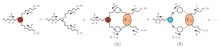
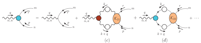
Figure 3: The coupled system of inhomogeneous BSEs for the three-gluon and ghost-gluon vertices, ${\rm{I}}\!\Gamma^{\alpha\mu\nu}(q,r,p)$ and ${\rm{I}}\!\Gamma^{\alpha}(q,r,p)$, respectively. Circles represent full propagators or vertices, while the orange ellipses correspond to four-point scattering kernels, ${\cal K}_{ij}$. The omitted diagrams contain five-point scattering kernels, associated with fully-dressed four-gluon vertices with incoming momentum $q$, which are neglected in our truncation scheme.

The starting point of this study is the BS version of the SDEs that govern the momentum evolution of the three-gluon vertex, ${\rm{I}}\!\Gamma_{\alpha\mu\nu}(q,r,p)$, and of the conventional ghost-gluon vertex, ${\rm{I}}\!\Gamma_{\alpha}(q,r,p)$, shown in Fig. 3. In particular, we replace (inside the loops) the tree-level vertices (with incoming momentum $q$) by their fully-dressed counterparts, modifying the corresponding multiparticle kernels ${\cal K}_{ij}$ accordingly, to avoid overcounting (see e.g., Fig. 7 of Aguilar et al. (2012)). The main advantage of this conversion is that various vertex renormalization constants, which otherwise would appear explicitly multiplying the corresponding diagrams, are naturally absorbed by the additional dressed vertices. Note that, in order to simplify the pertinent set of SDEs, we omit from our analysis the fully-dressed four-gluon vertices (with incoming momentum $q$), whose impact is expected to be subleading Williams et al. (2016); Huber (2020).

In what follows, we will introduce a longitudinally coupled massless pole also in the ghost-gluon vertex ${\rm{I}}\!\Gamma_{\alpha}(q,r,p)$, casting it into a form analogous to Eq. (9), and diagrammatically represented in Fig. 1, where the incoming gluon is $Q^{a}_{\alpha}$ . In particular, we set

$${\rm{I}}\!\Gamma_{\alpha}(q,r,p)=\Gamma_{\alpha}(q,r,p)+V_{\alpha}(q,r,p),$$ (59)

where $\Gamma_{\alpha}(r,p,q)$ denotes the pole-free component, while

$$V_{\alpha}(q,r,p)=\frac{q_{\alpha}}{q^{2}}C(q,r,p)\,,$$ (60)

describes the pole multiplied by the associated form factor.

Then, the BSEs of Fig. 3 may be written schematically as

$${\rm{I}}\!\Gamma^{\alpha\mu\nu}(q,r,p) = \Gamma_{\!0}^{\alpha\mu\nu}(q,r,p)-\frac{ig^{2}C_{\rm A}}{2}\int_{k}{\rm{I}}\!\Gamma^{\alpha\beta\gamma}(q,k,-s)\Delta_{\beta\rho}(k)\Delta_{\gamma\sigma}(s){\cal K}_{11}^{\mu\nu\sigma\rho}(r,p,s,-k)$$

$$+ig^{2}C_{\rm A}\int_{k}{\rm{I}}\!\Gamma^{\alpha}(q,k,-s)D(k^{2})D(s^{2}){\cal K}_{12}^{\mu\nu}(r,p,s,-k)\,,$$

$${\rm{I}}\!\Gamma^{\alpha}(q,r,p) = \Gamma_{\!0}^{\alpha}(q,r,p)-\frac{ig^{2}C_{\rm A}}{2}\int_{k}{\rm{I}}\!\Gamma^{\alpha\beta\gamma}(q,k,-s)\Delta_{\beta\rho}(k)\Delta_{\gamma\sigma}(s){\cal K}_{21}^{\sigma\rho}(r,p,s,-k)$$ (61)

$$-\frac{ig^{2}C_{\rm A}}{2}\int_{k}{\rm{I}}\!\Gamma^{\alpha}(q,k,-s)D(k^{2})D(s^{2}){\cal K}_{22}(r,p,s,-k)\,,$$

where $\Gamma_{\!0}^{\alpha}(q,r,p)=r^{\alpha}$ is the tree level ghost-gluon vertex, $s:=k+q$, and we introduce the notation

$$\int_{k}:=\frac{1}{(2\pi)^{4}}\int\!\!d^{4}k\,,$$ (62)

for the integral measure. In Eq. (62), the use of a symmetry-preserving regularization scheme is implicitly assumed.

Next, we decompose the vertices in Eq. (61) according to Eqs. (24) and (59). Given that ${\rm{I}}\!\Gamma_{\alpha\mu\nu}(q,r,p)$ contains poles in all channels, $q_{\alpha}$, $r_{\mu}$, and $p_{\nu}$, we isolate the pole in $q_{\alpha}$ by contracting the first line of Eq. (61) with $P^{\mu\delta}(r)P^{\nu}_{\delta}(p)$. Then, using Eqs. (25) and (26) we find that

$$P^{\mu\delta}(r)P^{\nu}_{\delta}(p)V_{\alpha\mu\nu}(q,r,p)=\frac{q_{\alpha}}{q^{2}}P^{\mu\delta}(r)P^{\nu}_{\delta}(p)\left[g_{\mu\nu}C_{1}(q,r,p)+q_{\mu}q_{\nu}C_{5}(q,r,p)\right]\,,$$ (63)

so that the only pole terms on the l.h.s. of Eq. (61) are those containing $C_{1}$ and $C_{5}$. In addition, due to the transversality of the Landau gauge gluon propagator, Eq. (63) [with $q\to q$, $r\to k$, and $p\to-s$] can be used inside the integral of diagram ($a$); again, only $C_{1}(q,k,-s)$ and $C_{5}(q,k,-s)$ survive. Exactly the same situation is reproduced inside diagram ($c$).

The following step is to multiply Eq. (61) by $q^{2}$ and expand around $q=0$. In doing so, we recall Eqs. (34) and (40), and the analogous relations for $C(q,r,p)$, namely

$$C(0,r,-r)=0\,,$$ (64)

and

$$\left[\frac{\partial C(q,r,p)}{\partial q^{\alpha}}\right]_{q=0}\!\!\!\!\!=2r_{\alpha}\,{\mathcal{C}}(r^{2})\,,\qquad{\mathcal{C}}(r^{2}):=\left[\frac{\partial C(q,r,p)}{\partial p^{2}}\right]_{q=0}\!\!\!\!\!\,.$$ (65)

Then, as $q\to 0$, the term proportional to $C_{5}$ in Eq. (63) is of higher order in $q$ and drops out.

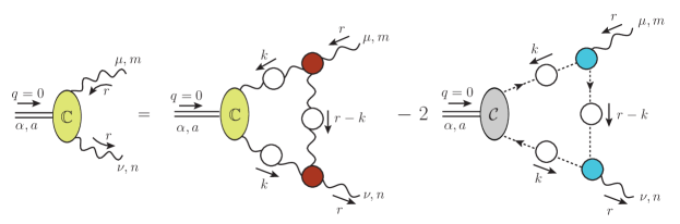
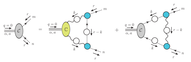
Figure 4: The coupled system of BSEs governing the evolution of ${\mathbb{C}}(r^{2})$ and ${\mathcal{C}}(r^{2})$.

Consequently, we obtain a set of homogeneous equations involving only ${\mathbb{C}}(r^{2})$ and ${\mathcal{C}}(r^{2})$. Specifically, we find

$$3(q\cdot r){\mathbb{C}}(r^{2}) = -\frac{ig^{2}C_{\rm A}}{2}\int_{k}(q\cdot k){\mathbb{C}}(k^{2})\Delta^{2}(k^{2})P_{\rho\sigma}(k)P_{\mu\nu}(r){\cal K}_{11}^{\mu\nu\sigma\rho}(r,-r,k,-k)$$

$$+ig^{2}C_{\rm A}\int_{k}(q\cdot k)\,{\mathcal{C}}(k^{2})D^{2}(k^{2})P_{\mu\nu}(r){\cal K}_{12}^{\mu\nu}(r,-r,k,-k)\,,$$

$$(q\cdot r)\,{\mathcal{C}}(r^{2}) = -\frac{ig^{2}C_{\rm A}}{2}\int_{k}(q\cdot k)\,{\mathbb{C}}(k^{2})\Delta^{2}(k^{2})P_{\sigma\rho}(k){\cal K}_{21}^{\sigma\rho}(r,-r,k,-k)$$ (66)

$$-\frac{ig^{2}C_{\rm A}}{2}\int_{k}(q\cdot k)\,{\mathcal{C}}(k^{2})D^{2}(k^{2}){\cal K}_{22}(r,-r,k,-k)\,,$$

where we have used $P^{\mu}_{\mu}(r)=3$. Finally, the remaining common factor of $q$ can be eliminated straightforwardly, by making use of the basic formula

$$\int_{k}(q\cdot k)\,F(k,r)=\frac{(q\cdot r)}{r^{2}}\int_{k}(r\cdot k)\,F(k,r)\,.$$ (67)

Finally, we approximate the four-point scattering kernels ${\cal K}_{ij}$ by their one-particle exchange diagrams (see e.g., Figs. 4 and 5 of Aguilar et al. (2018)), thus reducing the BSEs governing ${\mathbb{C}}(r^{2})$ and ${\mathcal{C}}(r^{2})$ to the form shown in Fig. 4; the corresponding algebraic expressions are given in Eq. (76).

We observe that the system of integral equations reached in Eq. (66) is the (approximate) BSE that governs the formation of massless colored bound states ($q^{2}=0$), as announced. Thus, the function ${\mathbb{C}}(r^{2})$, connected with the displacement of the WI in Eq. (58), emerges naturally as the wave function associated with the pole formation of a colored two-gluon bound state.

We point out that, in addition to the lattice propagators given in Appendix C, the numerical evaluation of the BSEs requires information on various form factors of the pole-free vertices $\Gamma_{\alpha\mu\nu}(q,r,p)$ and $\Gamma_{\alpha}(q,r,p)$; for details, see Appendix A.

We emphasize that, due to the homogeneity and linearity of Eq. (76), the overall scale of the solution is undetermined: the multiplication of a given solution by an arbitrary real constant yields another solution. For the purposes of the present work, this ambiguity was resolved by matching the BSE prediction for ${\mathbb{C}}(r^{2})$ to the result obtained from the WI in the next section. The solutions found for ${\mathbb{C}}(r^{2})$ and ${\mathcal{C}}(r^{2})$ after the implementation of this scale-fixing procedure, denoted as ${\mathbb{C}}_{\star}(r^{2})$ and ${\mathcal{C}}_{\star}(r^{2})$, respectively, are shown in Fig. 5. Note that ${\mathbb{C}}_{\star}(r^{2})$ is considerably larger in magnitude than ${\mathcal{C}}_{\star}(r^{2})$, in agreement with the original study presented in Aguilar et al. (2018).

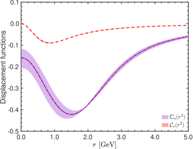
Figure 5: The solutions for ${\mathbb{C}}_{\star}(r^{2})$ (purple dot-dashed) and ${\mathcal{C}}_{\star}(r^{2})$ (red dashed) obtained from the coupled BSE system of Eq. (76). The origin of the error bands is the propagation of the error associated with $\mathit{L}_{{sg}}(r^{2})$, used to calibrate the three-gluon vertex inputs. The band of ${\mathcal{C}}_{\star}(r^{2})$ turns out to be very thin and barely visible.

VI Displacement function from the Ward identity

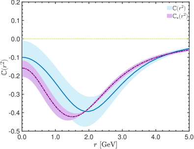
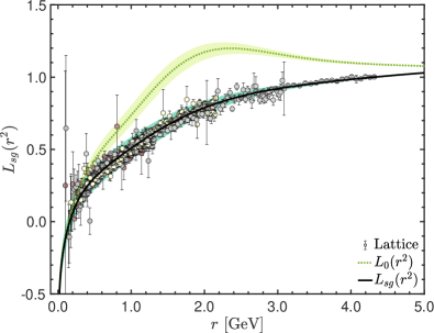
Figure 6: Left: ${\mathbb{C}}(r^{2})$ obtained from Eq. (58) (blue continuous curve) compared to the BSE prediction, ${\mathbb{C}}_{\star}(r^{2})$, based on Eq. (76) (purple dot-dashed). Right: Lattice data of Aguilar et al. (2021a) for $\mathit{L}_{{sg}}(r^{2})$ (points), compared to the fit of Eq. (106) (black continuous), and the null hypothesis prediction, $\mathit{L}_{0}(r^{2})$, of Eq. (68) (green dotted). The band around $\mathit{L}_{{sg}}(r^{2})$ is delimited by the functions $\mathit{L}_{{sg}}^{\pm}(r^{2})$ of Eq. (107).

We next determine the signal for ${\mathbb{C}}(r^{2})$ that emerges from the corresponding WI, and discuss its statistical significance with respect to the null hypothesis, namely the case where ${\mathbb{C}}(r^{2})$ would vanish identically.

To that end, we substitute on the r.h.s. of Eq. (58) appropriate expressions for all quantities appearing there. In particular, we employ physically motivated fits to lattice results for the gluon propagator, the ghost dressing function, and $\mathit{L}_{{sg}}(r^{2})$, given in Appendix C. Instead, the function ${\cal W}(r^{2})$ is computed from its own SDE, as described in Appendix B; the resulting ${\cal W}(r^{2})$ is shown as the blue solid line and error band in the right panel of Fig. 11.

The outcome of this operation is clearly nonvanishing: the resulting ${\mathbb{C}}(r^{2})$ is shown in the left panel of Fig. 6 as the blue continuous curve, which is distinctly separated from the null hypothesis case, indicated by the green dotted line. The blue band surrounding the central result indicates the errors assigned to ${\mathbb{C}}(r^{2})$, through the propagation of the corresponding errors associated with the ingredients entering on the r.h.s. of Eq. (58).

In the same figure we plot the ${\mathbb{C}}_{\star}(r^{2})$ of Fig. 5, in order to facilitate the direct comparison. We observe an excellent agreement in the overall shapes of ${\mathbb{C}}_{\star}(r^{2})$ and ${\mathbb{C}}(r^{2})$. Their main difference is the position and depth of the minimum: for ${\mathbb{C}}(r^{2})$ we have $r_{{\scriptscriptstyle\rm min}}=1.95\begin{subarray}{c}+0.07\\ -0.10\end{subarray}\,$ and ${\mathbb{C}}(r_{{\scriptscriptstyle\rm min}}^{2})=-0.39\pm 0.08$, while for ${\mathbb{C}}_{\star}(r^{2})$ we find $r_{{\scriptscriptstyle\rm min}}=1.50\begin{subarray}{c}+0.12\\ -0.13\end{subarray}\,$ and ${\mathbb{C}}_{\star}(r_{{\scriptscriptstyle\rm min}}^{2})=-0.42\pm 0.02$.

In order to provide an estimate of the statistical significance of the above signal, we find it advantageous to recast our analysis in terms of the quantity $\mathit{L}_{{sg}}(r^{2})$, thus capitalizing on the detailed error analysis applied to the lattice data of Aguilar et al. (2021a). Specifically, from the WI of Eq. (58) we will determine the form that $\mathit{L}_{{sg}}(r^{2})$ would have if the null hypothesis were true, and quantify its deviation from the actual lattice data.

Thus, setting ${\mathbb{C}}(r^{2})=0$ into Eq. (58), we obtain the null hypothesis prediction for $\mathit{L}_{{sg}}(r^{2})$, which we denote by $\mathit{L}_{0}(r^{2})$, given by

$$\mathit{L}_{0}(r^{2})=F(0)\left\{\frac{{\cal W}(r^{2})\Delta^{-1}(r^{2})}{r^{2}}+\widetilde{Z}_{1}\left[\Delta^{-1}(r^{2})\right]^{\prime}\right\}\,.$$ (68)

Substituting on the r.h.s. of Eq. (68) the same ingredients as before, we obtain the $\mathit{L}_{0}(r^{2})$ shown as the green dotted line on the right panel of Fig. 6. The green band enveloping $\mathit{L}_{0}(r^{2})$ captures the error propagated from ${\cal W}(r^{2})$; it is obtained by using as inputs into Eq. (68) the curves delimiting the blue band in the right panel of Fig. 11.

The results shown in Fig. 6 demonstrate that the statistical error of the lattice cannot account for the discrepancy between $\mathit{L}_{{sg}}(r^{2})$ and $\mathit{L}_{0}(r^{2})$; evidently, the null hypothesis is strongly disfavored.

In order to quantify the above statement, we adopt the following procedure.

(i) At every data point, denoted by the index $i$ and located at the momentum $r_{i}$, we consider the standard error in the lattice data for $\mathit{L}_{{sg}}$, denoted by $\rho_{i}$, and the propagated error in the null hypothesis prediction, $\mathit{L}_{0}(r_{i})$, denoted by $\tau_{i}$, as shown in the inset of the left panel of Fig. 7.

(ii) These errors are found to be correlated. Specifically, when using a higher $\mathit{L}_{{sg}}(r^{2})$ as input in Eq. (68), we obtain a lower $\mathit{L}_{0}(r^{2})$. Hence, the total error, denoted by $\sigma_{i}$, is given by $\sigma_{i}:=\rho_{i}+\tau_{i}$. Note that the $\sigma_{i}$ so defined is larger than the corresponding errors combined in quadrature, i.e., $\sqrt{\rho_{i}^{2}+\tau_{i}^{2}}$, which would be appropriate if the $\rho_{i}$ and $\tau_{i}$ were independent.

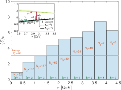
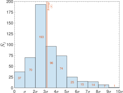
Figure 7: Left: $\langle\,{\delta}\,\rangle_{k}$, the average standard deviation of all point belonging to the $k$-th bin of momentum, plotted as a function of the momentum $r$. The inset describes the definition of the local individual deviations $\rho_{i}$ and $\tau_{i}$, which are combined in a total correlated error $\sigma_{i}=\rho_{i}+\tau_{i}$, valid for any given point, as described in the text, items (i) - (iii). Right: The distribution of all available points into bins of a given standard deviation. In both figures, the orange line represents the total average, $\langle\,\delta\,\rangle=3.1\sigma$.

(iii) Next, we measure the distance $\Delta L_{i}:=|\mathit{L}_{0}(r_{i}^{2})-\mathit{L}_{{sg}}(r_{i}^{2})|$, also shown in the inset of the left panel of Fig. 7, and then divide it by the corresponding total error, $\sigma_{i}$. The resulting ratio, ${\delta}_{i}:=\Delta L_{i}/\sigma_{i}$, measures the point-by-point deviation between the two curves, computed in units of the $\sigma$ (standard deviation) assigned to every given data point.

(iv) The entire momentum range considered, [$0,4.5$] GeV, is divided into nine equal bins of length $0.5$ GeV; thus, the $k$-th bin is defined as the interval [$0.5\,(k-1),0.5\,k$] GeV, $k=1,\cdots,9$. In addition, we denote by $N_{k}$ the total number of points in the $k$-th bin; we have $N_{k}=(52,167,157,69,40,24,10,7,6)$, accounting for a total of $N=532$ lattice points.

(v) Then, we compute the average value of the ratio ${\delta}_{i}$ within the $k$-th bin, and denote the answer by $\langle\,{\delta}\,\rangle_{k}$, namely

$$\langle\,{\delta}\,\rangle_{k}=\frac{1}{N_{k}}\sum_{i=n_{k}+1}^{n_{k}+N_{k}}\!\!{\delta}_{i}\,,\qquad\mathrm{with}\,\,\,\,n_{k}=\sum_{\ell=1}^{k-1}N_{\ell}\,.$$ (69)

(vi) Finally, the total average, $\langle\,\delta\,\rangle$, is defined as

$$\langle\,{\delta}\,\rangle=\frac{1}{N}\sum_{i=1}^{N}{\delta}_{i}\,,$$ (70)

and furnishes a measure of the global deviation between the signal [$\mathit{L}_{{sg}}(r^{2})$] and the null hypothesis [$\mathit{L}_{0}(r^{2})$] curves.

The outcome of this procedure is displayed in the left panel of Fig. 7, where the quantity $\langle\,{\delta}\,\rangle_{k}$, obtained at step (v), is plotted for each bin. The value of $\langle\,{\delta}\,\rangle$, computed at step (vi), is $\langle\,{\delta}\,\rangle=3.1$, and is marked by the orange horizontal line.

As we can observe, the values of $\langle\,{\delta}\,\rangle_{k}$ for the bins with $r>1.5$ GeV are considerably higher than $\langle\,\delta\,\rangle$. In fact, for $r>2$ GeV the value of the corresponding $\langle\,{\delta}\,\rangle_{k}$ exceeds $5\sigma$; however, the available points in this interval are relatively few. The sizable signal found above $2$ GeV may be understood as follows. First, near $2$ GeV, the lattice curve $\mathit{L}_{{sg}}$ is the farthest away from its null hypothesis counterpart, $\mathit{L}_{0}$, leading to large values for the $\Delta L_{i}$ [see (iii)] in that region. Second, for $r>3$ GeV, the $\mathit{L}_{{sg}}(r^{2})$ and $\mathit{L}_{0}(r^{2})$ approach each other; nevertheless, since the lattice error bars become very small in the UV, a rather strong signal emerges.

We next consider the distribution of all available points into bins of a given standard deviation, regardless of the momentum assigned to each point. The length of each bin is one $\sigma$, the $j$-th bin ($j=1,...10$) contains all points whose standard deviation lies in the interval $[j-1,\,j]\sigma$, and we denote the number of these points by ${\widetilde{N}}_{j}$. The result of this grouping is shown in the right panel of Fig. 7. We observe that, the largest number of points (193) is contained in the $[2-3]\sigma$ bin, while 133 points, corresponding to $25\%$ of the total number, are at or above the $5\sigma$ significance level. The average of $3.1\sigma$ is denoted by the orange vertical line.

Given that the truncation error in ${\cal W}(r^{2})$ is the main uncertainty in our analysis, we end this section by considering two interesting limiting cases associated with this function.

First, given the clear proximity between ${\mathbb{C}}(r^{2})$ and ${\mathbb{C}}_{\star}(r^{2})$, shown in the left panel of Fig. 6, it is tempting to ask whether a small modification in the shape of ${\cal W}(r^{2})$ could make ${\mathbb{C}}(r^{2})$ and ${\mathbb{C}}_{\star}(r^{2})$ agree perfectly.

To that end we substitute ${\cal W}(r^{2})\to{{\cal W}}_{\star}(r^{2})$ and ${\mathbb{C}}(r^{2})\to{\mathbb{C}}_{\star}(r^{2})$ in Eq. (58) to obtain the function ${{\cal W}}_{\star}(r^{2})$ necessary to reproduce ${\mathbb{C}}_{\star}(r^{2})$. Specifically,

$${{\cal W}}_{\star}(r^{2})=r^{2}\Delta(r^{2})\left\{\frac{\mathit{L}_{{sg}}(r^{2})-{\mathbb{C}}_{\star}(r^{2})}{F(0)}-\widetilde{Z}_{1}\left[\Delta^{-1}(r^{2})\right]^{\prime}\right\}\,.$$ (71)

The ${{\cal W}}_{\star}(r^{2})$ resulting from Eq. (71) is shown as the purple dot-dashed curve and the associated error band in Fig. 8, where it is compared to the SDE result for ${\cal W}(r^{2})$. Indeed, we observe that a minor adjustment in the shape of ${\cal W}(r^{2})$ would bring ${\mathbb{C}}(r^{2})$ and ${\mathbb{C}}_{\star}(r^{2})$ to a perfect agreement.

Second, it is instructive to consider what would happen if the null hypothesis were valid, and all resulting mismatches were to be absorbed exclusively into a modification of ${\cal W}(r^{2})$, to be denoted by ${{\cal W}}_{0}(r^{2})$.

Setting ${\mathbb{C}}(r^{2})=0$ and ${\cal W}(r^{2})\to{{\cal W}}_{0}(r^{2})$ into Eq. (58), we obtain

$${{\cal W}}_{0}(r^{2})=r^{2}\Delta(r^{2})\left\{\frac{\mathit{L}_{{sg}}(r^{2})}{F(0)}-\widetilde{Z}_{1}\left[\Delta^{-1}(r^{2})\right]^{\prime}\right\}\,.$$ (72)

In Fig. 8 we show ${{\cal W}}_{0}(r^{2})$ as the green dotted curve. The band around it represents the propagated error of the lattice $\mathit{L}_{{sg}}(r^{2})$; it is obtained by substituting $\mathit{L}_{{sg}}(r^{2})$ in Eq. (72) by the $\mathit{L}_{{sg}}^{\pm}(r^{2})$ of Eq. (107).

We note that the ${\cal W}(r^{2})$ obtained from the SDE (blue solid curve) is comfortably separated from ${{\cal W}}_{0}(r^{2})$. In fact, our attempts to obtain solutions of the SDE in the vicinity of ${{\cal W}}_{0}(r^{2})$ have been unavailing.

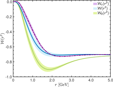
Figure 8: Direct comparison between the SDE result for ${\cal W}(r^{2})$ (blue continuous) and the ${{\cal W}}_{\star}(r^{2})$ (purple dot-dashed) that imposes the equality between the ${\mathbb{C}}(r^{2})$ obtained from the WI and the BSE. Also shown is the ${{\cal W}}_{0}(r^{2})$ that corresponds to the null hypothesis (green dotted). The bands around each curve correspond to the propagated errors from the lattice $\mathit{L}_{{sg}}(r^{2})$.

VII Discussion and Conclusions

In the present work we have investigated in detail a characteristic feature that is intimately linked with the onset of the Schwinger mechanism in QCD, and the ensuing emergence of an effective gluon mass scale. The action of this mechanism relies on the inclusion of massless longitudinal poles in the fundamental vertices of the theory, which participate nontrivially in the realization of the corresponding STIs. This, in turn causes a distinct displacement to the WI satisfied by the pole-free part of the vertices involved, quantified by the function ${\mathbb{C}}(r^{2})$, which is formally identical to the bound-state wave function that governs the dynamical formation of the massless poles. We have computed ${\mathbb{C}}(r^{2})$ for the case of the three-gluon vertex in two distinct ways: by solving the corresponding BSE and by appropriately combining the ingredients appearing in the non-Abelian WI. In both cases we have relied predominantly on results obtained from lattice simulations, with the exception of the special function ${\cal W}(r^{2})$, which was determined from an SDE. The results found for ${\mathbb{C}}(r^{2})$ are clearly nonvanishing and in excellent mutual agreement, providing additional support to the details of the general dynamical picture put forth in a series of articles. In particular, the dual r$\hat{\textrm{o}}$le played by ${\mathbb{C}}(r^{2})$ is especially noteworthy, hinting towards deeper connections that have yet to be unraveled.

It is important to stress that the computation of the null hypothesis, presented in Sec. VI, proceeds by assuming that all inputs of Eq. (68) retain their known form; in particular, salient features, such as the saturation of the gluon propagator and the ghost dressing function, persist unaltered. In that sense, this specific implementation probes the compatibility between the lattice results and the absence of a displacement in the non-Abelian WI of the three-gluon vertex. Seen from this point of view, one might state that this particular possibility is excluded at the level of $3.1\sigma$.

As mentioned in Appendix A, the value of $\alpha_{s}$ that corresponds to the eigenvalue of the system is $\alpha_{s}=0.63$, which is considerably different from the value $\alpha_{s}=0.27$ found within the “asymmetric” MOM scheme that we employ. The discrepancy may be interpreted as a truncation artifact, given that the corresponding BSE kernels has been approximated by their one-particle exchange diagrams, as depicted in Fig. 4. In addition, the expressions employed for the fully dressed vertices comprising these kernels contain a certain amount of uncertainty. Quite interestingly, a preliminary numerical exploration indicates that minor modifications of the kernel affect the value of $\alpha_{s}$ considerably, without practically modifying the form of the solution found for ${\mathbb{C}}_{\star}(r^{2})$ and ${\mathcal{C}}_{\star}(r^{2})$. This observation suggests that, while the decrease of $\alpha_{s}$ towards its MOM value may require a more refined knowledge of the corresponding BSE kernels, the obtained solutions should be considered as fairly reliable.

The proximity between the ${\cal W}(r^{2})$, computed in Appendix B, and the ${{\cal W}}_{\star}(r^{2})$ obtained from Eq. (71), suggest that minor modifications of the inputs used for the SDE of Eq. (87) might lead to an even better coincidence. In this context, it is interesting to point out that the determination of the transverse form factors $Y_{i}$ (see item (iii) in Appendix B) is subject to a considerable uncertainty, originating from the approximations implemented to the complicated SDE satisfied by the three-gluon vertex (Fig. 6 in Aguilar et al. (2021a)). Given the relevance of ${\cal W}(r^{2})$ for the systematic scrutiny of the Schwinger mechanism, as exposed in the present work, it may be worthwhile revisiting this particular computation.

As mentioned below Eq. (28), the Schwinger mechanism induces poles also in the ghost-gluon kernel, $H_{\mu\nu}(r,q,p)$. This may be understood qualitatively by considering the diagrams ($d_{1}$) and ($d_{2}$) in Fig. 10: the fully-dressed ghost-gluon and three-gluon vertices (with Lorentz index $\nu$ and incoming momentum $p$) contain poles, which are transmitted to the form factors of $H_{\mu\nu}(r,q,p)$ associated with the tensorial structures $p_{\nu}p_{\mu}$ and $p_{\nu}r_{\mu}$. It would be important to compute in detail the pole structure of $H_{\mu\nu}(r,q,p)$, especially in view of the STI $r^{\mu}H_{\mu\nu}(r,q,p)=\Gamma_{\nu}(p,r,q)$, which links nontrivially the form factors of $H_{\mu\nu}(p,r,q)$ and $\Gamma_{\mu}(p,r,q)$, in general, and the corresponding pole terms, in particular. Specifically, one may explore how accurately the appropriate combination of pole terms coming from $H_{\mu\nu}(p,r,q)$ will reproduce the corresponding term contained in $\Gamma_{\mu}(p,r,q)$. We hope to undertake such a study in the near future.

The scale ambiguity associated with the BSE amplitudes ${\mathbb{C}}(r^{2})$ and ${\mathcal{C}}(r^{2})$ results in from considering only the leading order terms of the BSEs in an expansion around $q=0$, which furnishes homogeneous linear equations. In general kinematics, however, the presence of inhomogeneous terms in the BSEs resolves this ambiguity. As such, the scales of ${\mathbb{C}}(r^{2})$ and ${\mathcal{C}}(r^{2})$ can be fixed by taking the $q=0$ limit of the solution of the corresponding inhomogeneous BSEs, treated beyond leading order in $q$. In the context of conventional bound states, this procedure is well understood Nakanishi (1969) and explicit scale-setting equations have been derived, which are sometimes referred to as “canonical normalization condition” Maris and Roberts (1997); Blank and Krassnigg (2011). It is our intention to pursue this point in an upcoming study, and settle dynamically the scale of the corresponding solutions.

Appendix A Technical details on the BSE system

In this Appendix we present details related to the numerical treatment of the BSE system formed by ${\mathbb{C}}(r^{2})$ and ${\mathcal{C}}(r^{2})$, shown in Fig. 4.

For the Bose symmetric three-gluon vertex appearing in the diagrams of Fig. 4 we employ the tensor basis of Ball-Chiu Ball and Chiu (1980); Aguilar et al. (2019c),

$$\Gamma^{\alpha\mu\nu}(q,r,p)=\sum_{i=1}^{10}X_{i}(q,r,p)\ell_{i}^{\alpha\mu\nu}+\sum_{i=1}^{4}Y_{i}(q,r,p)t_{i}^{\alpha\mu\nu}\,,$$ (73)

where the explicit form of the basis tensors $\ell_{i}^{\alpha\mu\nu}$ and $t_{i}^{\alpha\mu\nu}$ is given in Eqs. (3.4) and (3.6) of Aguilar et al. (2019c). At tree level, $X_{1}^{(0)}=X_{4}^{(0)}=X_{7}^{(0)}=1$, while all other $X_{i}^{(0)}$ and $Y_{i}^{(0)}$ vanish.

It is convenient to introduce the transversely projected vertex, $\overline{\Gamma}_{\alpha\mu\nu}(q,r,p)$, defined as

$$\overline{\Gamma}_{\,\alpha\mu\nu}(q,r,p):=P^{\alpha^{\prime}}_{\alpha}(q)P^{\mu^{\prime}}_{\mu}(r)P^{\nu^{\prime}}_{\nu}(p)\Gamma_{\alpha^{\prime}\mu^{\prime}\nu^{\prime}}(q,r,p)\,.$$ (74)

Similarly, the tensorial decomposition of the vertex $\Gamma_{\mu}(q,r,p)$ is given by

$$\Gamma_{\mu}(q,r,p)=r_{\mu}B_{1}(r,p,q)+q_{\mu}B_{2}(r,p,q)\,;$$ (75)

at tree level, $B_{1}^{(0)}=1$ and $B_{2}^{(0)}=0$. The ghost-anti-ghost symmetry of $\Gamma_{\mu}(q,r,p)$ in the Landau gauge implies that $B_{1}(r,p,q)=B_{1}(p,r,q)$.

Next, we pass to Euclidean space and employ spherical coordinates. For convenience, we define the variables $x:=r^{2}$, $y:=k^{2}$, and $u:=(r-k)^{2}=x+y-2\sqrt{xy}c_{\phi}$, with $\phi$ denoting the angle between the momenta $k$ and $r$, while $s_{\phi}:=\sin\phi$, $c_{\phi}:=\cos\phi$. Furthermore, we parametrize scalar form factors, such as $B_{1}(q,r,p)$, in terms of the squares of their first two arguments and the angle between them, e.g., $B_{1}(-r,k,r-k)\to B_{1}(x,y,\pi-\phi)$. Then, the final set of BSEs reads

$${\mathbb{C}}(x) = \lambda\left[\int_{0}^{\infty}\!\!\!dy\,y\sqrt{xy}\Delta^{2}(y){\mathbb{C}}(y)\int_{0}^{\pi}\!\!\!d\phi s_{\phi}^{2}c_{\phi}\Delta(u){\cal N}(x,y,u)\right.$$

$$\left.\hskip 56.9055pt-2\int_{0}^{\infty}\!\!\!dy\sqrt{\frac{y}{x}}F^{2}(y){\mathcal{C}}(y)\int_{0}^{\pi}\!\!\!d\phi s_{\phi}^{4}c_{\phi}\frac{F(u)}{u}B_{1}^{2}(u,y,\chi)\right]\,,$$

$${\mathcal{C}}(x) = 3\lambda\left[\int_{0}^{\infty}\!\!\!dy\,y\sqrt{xy}\Delta^{2}(y){\mathbb{C}}(y)\int_{0}^{\pi}\!\!\!d\phi s_{\phi}^{4}c_{\phi}\frac{F(u)}{u}B_{1}^{2}(x,u,\theta)\right.$$ (76)

$$\left.\hskip 56.9055pt+\int_{0}^{\infty}\!\!\!dy\sqrt{xy}F^{2}(y){\mathcal{C}}(y)\int_{0}^{\pi}\!\!\!d\phi s^{4}_{\phi}c_{\phi}\frac{\Delta(u)}{u}B_{1}^{2}(x,y,\pi-\phi)\right]\,.$$

In the above equation,

$$\lambda:=\frac{\alpha_{s}C_{\rm A}}{12\pi^{2}}\,,$$ (77)

where $\alpha_{s}:=g^{2}/4\pi$. The angles $\chi$ and $\theta$ are given by

$$\chi=\cos^{-1}\left(\frac{\sqrt{x}\cos\phi-\sqrt{y}}{\sqrt{u}}\right)\,,\qquad\theta=\cos^{-1}\left(\frac{\sqrt{y}\cos\phi-\sqrt{x}}{\sqrt{u}}\right)\,.$$ (78)

Finally,

$${\cal N}(x,y,u):=-\frac{1}{x}\left[\overline{\Gamma}_{\,\alpha\beta\gamma}(-r,k,r-k)\overline{\Gamma}^{\,\alpha\beta\gamma}(-r,k,r-k)\right]_{\rm E}\,,$$ (79)

where the subscript “E” indicates that Eq. (79) is to be converted to Euclidean coordinates.

The ${\cal N}(x,y,u)$ of Eq. (79) can be written in terms of the form factors $X_{i}$ and $Y_{i}$ of Eq. (73); note that the $X_{i}$ with $i=2,5,8,10$ drop out, because they are annihilated by the transverse projection in Eq. (74).

Then, we obtain

$${\cal N}(x,y,u) = \frac{s^{2}_{\phi}}{2u^{2}x^{2}y}\left\{uT_{1}\left[T_{1}\left((u-x-y)^{2}+2xy\right)+4xy(T_{2}+T_{3})+4T_{4}(u-x-y)\right]\right.$$

$$+xT_{2}\left[T_{2}\left((u-x+y)^{2}+2uy)\right)+4uyT_{3}-4T_{4}(u-x+y)\right]$$

$$\left.+yT_{3}\left[T_{3}\left((u+x-y)^{2}+2ux\right)-4T_{4}(u+x-y)\right]+4T_{4}^{2}(u+x+y)\right\}\,,$$

where

$$T_{1} = -u(X_{1}-X_{4}-X_{7}+xyY_{1})-x(X_{1}-X_{4}+X_{7}-2yX_{3})-y(X_{1}+X_{4}-X_{7})\,,$$

$$T_{2} = u(X_{1}-X_{4}-X_{7}+2yX_{6}-xyY_{2})+x(X_{1}-X_{4}+X_{7})-y(X_{1}+X_{4}-X_{7})\,,$$

$$T_{3} = u(X_{1}-X_{4}-X_{7}+2xX_{9}-xyY_{3})-x(X_{1}-X_{4}+X_{7})+y(X_{1}+X_{4}-X_{7})\,,$$

$$T_{4} = \frac{1}{2}\left\{u^{2}(X_{1}-X_{4}-X_{7})-(x-y)\left[x(X_{1}-X_{4}+X_{7})-y(X_{1}+X_{4}-X_{7})\right]\right.$$ (81)

$$\left.+2u\left[x(X_{7}-yY_{4})+yX_{4}\right]\right\}\,,$$

and we suppress the functional dependence $X_{i}\equiv X_{i}(x,y,\pi-\phi)$ and $Y_{j}\equiv Y_{j}(x,y,\pi-\phi)$.

For the numerical evaluation of Eq. (76), in addition to the lattice propagators given in Appendix C, we need $B_{1}$, together with all $X_{i}$ and $Y_{i}$ that comprise ${\cal N}(x,y,u)$, in general kinematics. These form factors are obtained as follows:

(i) For the $B_{1}$ we employ recent results (see Fig. 6 of Aguilar et al. (2021c)), obtained from an SDE analysis that uses as inputs lattice data that have been cured from volume and discretization artifacts.

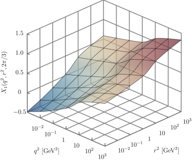
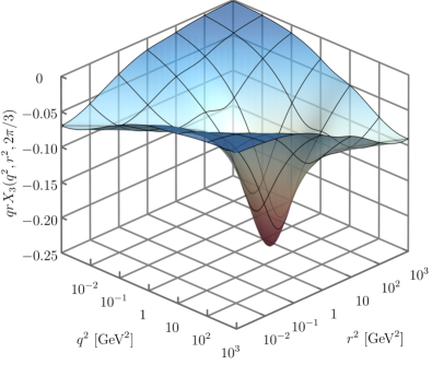
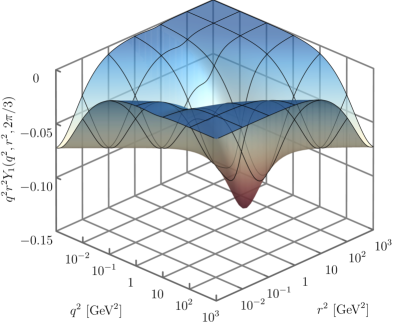
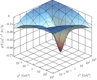
Figure 9: The three-gluon vertex form factors used in the BSE system: $X_{1}(q^{2},r^{2},2\pi/3)$ (top left), $qrX_{3}(q^{2},r^{2},2\pi/3)$ (top right), $q^{2}r^{2}Y_{1}(q^{2},r^{2},2\pi/3)$ (bottom left), and $qrY_{4}(q^{2},r^{2},2\pi/3)$ (bottom right).

(ii) The $X_{i}$ are obtained from the nonperturbative generalization of the Ball-Chiu solution; the relevant formulas are given in Eq. (3.11) of Aguilar et al. (2019c), and involve the ghost dressing function, the kinetic term of the gluon propagator, and certain components of the ghost-gluon kernel. Note that the inputs have been calibrated to exactly reproduce the lattice projection $\mathit{L}_{{sg}}(r^{2})$, through the relation

$$\mathit{L}_{{sg}}(r^{2})=X_{1}(r^{2},r^{2},\pi)-r^{2}X_{3}(r^{2},r^{2},\pi)\,.$$ (82)

In this indirect way, the error bars assigned to the lattice calculation of $\mathit{L}_{{sg}}(r^{2})$, encompassed by the functions $\mathit{L}_{{sg}}^{\pm}(r^{2})$ of Eq. (107), find their way into our BSE determination of ${\mathbb{C}}(r^{2})$ and ${\mathcal{C}}(r^{2})$, giving rise to the errors band indicated in Fig. 6

(iii) For the transverse components $Y_{i}$, which cannot be deduced from the fundamental STIs, we resort to a SDE determination, along the lines of the analysis presented in Aguilar et al. (2021a); see, in particular, Fig. 6 therein.

(iv) The results for $X_{1}(q^{2},r^{2},\theta)$, $qrX_{3}(q^{2},r^{2},\theta)$, $q^{2}r^{2}Y_{1}(q^{2},r^{2},\theta)$, and $qrY_{4}(q^{2},r^{2},\theta)$ are shown in Fig. 9, for the special case $\theta=2\pi/3$; $q$ and $r$ denote now the magnitudes of the corresponding Euclidean momenta.

(v) By virtue of the Bose symmetry of the three-gluon vertex, the remaining form factors of the three-gluon vertex entering in Eq. (79) can be obtained from those shown in Fig. 9 by appropriate permutations of their arguments, as explained in Aguilar et al. (2019c).

Employing the ingredients described above, we solve the coupled system of BSEs of Eq. (76) numerically, obtaining the ${\mathbb{C}}(r^{2})$ and ${\mathcal{C}}(r^{2})$ shown in Fig. 5, together with the corresponding error estimates.

Since Eq. (76) does not have an inhomogeneous term and is linear in ${\mathbb{C}}(r^{2})$ and ${\mathcal{C}}(r^{2})$, it corresponds to an eigenvalue problem. The resulting eigenvalues correspond to $\alpha_{s}=0.63\mp 0.05$, with signs opposite to those of the $\mathit{L}_{{sg}}^{\pm}(r^{2})$ error bands, i.e., using $X_{i}$ corresponding to a higher $\mathit{L}_{{sg}}(r^{2})$ leads to a smaller $\alpha_{s}$. In these results, the overall constant was determined by matching the BSE prediction for ${\mathbb{C}}(r^{2})$ to the result obtained from the WI, as explained in Sec. VI.

Appendix B Computation of ${\cal W}(r^{2})$

The function ${\cal W}(r^{2})$ is a central ingredient for our analysis, whose determination proceeds through the study of the corresponding SDE. In this Appendix we present the technical details related to this calculation, and discuss the validity of our approximations.

B.1 SDE, inputs, and solution

The starting point of our determination of ${\cal W}(r^{2})$ is the SDE for the ghost-gluon scattering kernel, $H_{\mu\nu}(r,q,p)$, shown in Fig. 10, which is truncated at the one-loop dressed level, retaining only diagrams $(d_{1})$ and $(d_{2})$. In the Landau gauge it is immediate to factor out of these two diagrams the ghost momentum $q$, in order to obtain $K_{\mu\nu\alpha}(r,q,p)$, in accordance with Eq. (36). Finally, recalling Eq. (38), ${\cal W}(r^{2})$ is obtained by isolating the $g_{\mu\nu}r_{\alpha}$ form factor of $K_{\mu\nu\alpha}(r,0,-r)$ and using Eq. (57).

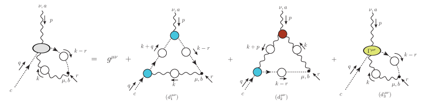
Figure 10: The SDE satisfied by the ghost-gluon scattering kernel, $H_{\mu\nu}(r,q,p)$.

Since a detailed derivation and renormalization of the ${\cal W}(r^{2})$ equation has been carried out in Sec. 6 of Ref. Aguilar et al. (2021b), here we only collect the main results. Specifically, we obtain the general expression

$${\cal W}(r^{2})={\cal W}_{1}(r^{2})+{\cal W}_{2}(r^{2})\,,$$ (83)

where ${\cal W}_{1}$ and ${\cal W}_{2}$ denote the contributions from diagrams $(d_{1})$ and $(d_{2})$ of Fig. 10, respectively, given by

$${\cal W}_{1}(r^{2}) = -\frac{ig^{2}C_{\rm A}\widetilde{Z}_{1}}{6}\int_{k}\Delta(k^{2})D(k^{2})D(t^{2})B_{1}(t,k,-r)B_{1}(k,0,-k)(r\cdot k)f(r,k)\,,$$

$${\cal W}_{2}(r^{2}) = -\frac{ig^{2}C_{\rm A}\widetilde{Z}_{1}}{6}\int_{k}\Delta(k^{2})\Delta(t^{2})D(t^{2})B_{1}(t,0,-t)r^{\alpha}\overline{\Gamma}^{\,\mu}_{\mu\alpha}(-r,k,t)\,,$$ (84)

where

$$f(r,k):=1-\frac{(k\cdot r)^{2}}{k^{2}r^{2}}\,,$$ (85)

and $\overline{\Gamma}$ is defined in Eq. (74). Note the appearance in Eq. (87) of $\widetilde{Z}_{1}$, defined below Eq. (36), which implements the renormalization of the SDE in the asymmetric MOM scheme Aguilar et al. (2021b).

To express Eq. (83) in Euclidean space, we use spherical coordinates and the kinematic variables $x$, $y$ and $u$ defined above Eq. (76). Then, using the Ball-Chiu tensor basis of Eq. (73) for the three-gluon vertex, we obtain

$${\cal W}(x)={\cal W}_{1}(x)+{\cal W}_{2}(x)\,,$$ (86)

with

$${\cal W}_{1}(x) = \lambda\widetilde{Z}_{1}\int_{0}^{\infty}\!\!\!\!\!dy\sqrt{xy}\Delta(y)F(y)B_{1}(y,0,0)\int_{0}^{\pi}\!\!\!d\phi\,c_{\phi}s_{\phi}^{4}\frac{F(u)}{u}B_{1}(u,y,\chi)\,,$$

$${\cal W}_{2}(x) = -2\lambda\widetilde{Z}_{1}\int_{0}^{\infty}\!\!\!\!\!dy\,y\sqrt{xy}\Delta(y)\int_{0}^{\pi}\!\!\!d\phi s_{\phi}^{4}\Delta(u)B_{1}(u,0,0)\frac{F(u)}{u^{2}}{\cal K}(x,y,u)\,,$$ (87)

where $\lambda$ is defined in Eq. (77), $\chi$ in Eq. (78), and we define the kernel ${\mathcal{K}}(x,y,u)$ as

$${\mathcal{K}}(x,y,u) := \sqrt{x\,y}(c_{\phi}^{2}+2)X_{1}+(y-c_{\phi}\sqrt{x\,y})c_{\phi}X_{4}+(x-c_{\phi}\sqrt{x\,y})c_{\phi}X_{7}-3c_{\phi}x\,yX_{3}$$ (88)

$$-c_{\phi}y\,uX_{6}-c_{\phi}x\,uX_{9}+\frac{1}{2}{c_{\phi}x\,y\,u}(3Y_{1}+Y_{2}+Y_{3})-u\sqrt{x\,y}\,Y_{4}\,,$$

where, again, $X_{i}\equiv X_{i}(x,y,\pi-\phi)$ and $Y_{j}\equiv Y_{j}(x,y,\pi-\phi)$.

Using the Bose symmetry relations involving permutations of arguments of the $X_{i}$ and $Y_{i}$, given by Eqs. (3.7) to (3.10) of Aguilar et al. (2019c), it is possible to show that $\mathcal{K}(x,y,u)$ is symmetric under the exchange of $x\leftrightarrow y$.

Then, for the gluon propagator $\Delta(r^{2})$ and the ghost dressing function $F(r^{2})$ we use the fits presented in Appendix C, while for the vertex form factors, $B_{1}$, $X_{i}$ and $Y_{i}$ we use the same inputs employed for the solution of the BSE of Eq. (76). Note that, as mentioned in Appendix C, all inputs are renormalized within the “asymmetric” MOM scheme, at the renormalization point $\mu=4.3$ GeV, for which $\alpha_{s}=0.27$.

With these ingredients, we obtain for ${\cal W}(r^{2})$ the blue continuous line shown in the right panel of Fig. 11. The blue band around it corresponds to error propagated from the uncertainty in the lattice $\mathit{L}_{{sg}}(r^{2})$, through the same procedure explained in item (ii) of Section A.

Given that ${\cal W}(r^{2})$ is one of the main ingredients in the analysis of Eq. (58), it is important to consider in more detail the uncertainty in our SDE determination of this function. It turns out that the contribution ${\cal W}_{1}(r^{2})$ of Eq. (87) is negligible in comparison to ${\cal W}_{2}(r^{2})$ (see Fig. 7 of Aguilar et al. (2021b)), except for $r<0.5$ GeV, where ${\cal W}_{2}(r^{2})$ decreases significantly. Furthermore, diagram $(d_{3})$ of Fig. 10, with the four-particle correlation function $\Gamma_{\mu\sigma}$ nested in it, is known to affect the ghost-gluon vertex only by $2\%$ Huber (2017); thus, its omission is expected to have an insignificant effect on ${\cal W}(r^{2})$. Therefore, the main uncertainty originates from the term ${\cal W}_{2}(r^{2})$ of Eq. (87), and is related to our incomplete knowledge of the form factors $X_{i}$ and $Y_{i}$ for general kinematics.

In this regard, an examination of the integrand of ${\cal W}_{2}(r^{2})$ in Eq. (87) shows that this contribution is dominated by the projection $\mathit{L}_{{sg}}(r^{2})$ of the full three-gluon vertex that it contains. In turn, this observation suggests that the SDE determination of ${\cal W}(r^{2})$ should be fairly accurate provided that the Ansatz employed for the general kinematics three-gluon vertex reproduces in the soft-gluon limit the $\mathit{L}_{{sg}}(r^{2})$ obtained on the lattice Aguilar et al. (2021a).

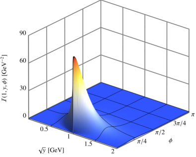
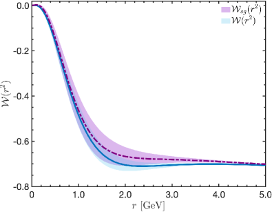
Figure 11: Left: The integrand of ${\cal W}_{2}(x)$, ${\cal I}(x,y,\phi)$, given by Eq. (89), for $x=1$ GeV². Note that its maximum occurs when $y$ is first set to $y=x=1$ GeV and then $\phi=0$, corresponding to $u=0$. ${\cal I}(x,y,\phi)$ is intensely peaked around the maximum, dropping rapidly to zero away from it. Right: Comparison of ${\cal W}(r^{2})$, obtained with Eq. (86) (blue solid line), to ${{\cal W}}_{{sg}}(r^{2})$, obtained with the replacement (94) into Eq. (86) (purple dot-dashed line). The bands correspond to propagated error from the lattice $\mathit{L}_{{sg}}(r^{2})$ of Aguilar et al. (2021a).

B.2 A closer look at the SDE kernel

To elucidate this last point, denote by ${\cal I}(x,y,\phi)$ the integrand of ${\cal W}_{2}(x)$ in Eq. (87), i.e.,

$${\cal I}(x,y,\phi):=s_{\phi}^{4}y\sqrt{xy}\Delta(y)\Delta(u)\frac{F(u)}{u^{2}}B_{1}(u,0,0){\cal K}(x,y,u)\,.$$ (89)

Then, since $F(u)$ and, especially, $\Delta(u)$ are decreasing functions of $u$, the term $\Delta(u)F(u)/u^{2}$ in the second line of Eq. (89) causes the ${\cal I}(x,y,\phi)$ to decrease rapidly at large $u$. Hence, ${\cal W}_{2}(x)$ should be dominated by the small $u$ region of its integrand.

Next, recalling that $u=x+y-2\sqrt{xy}c_{\phi}$, we note that $u=0$ occurs when $y=x$ and $\phi=0$ simultaneously. Also, we emphasize that, in spite of the presence of the factor $u^{2}$ in the denominator, Eq. (89) is finite at $u=0$, due to the vanishing of $s^{4}_{\phi}$ when $\phi=0$.

In the left panel of Fig. 11 we plot ${\cal I}(x,y,\phi)$ for $x=1$ GeV² and general $y$ and $\phi$, using the general kinematics $X_{i}$ and $Y_{i}$ of Fig. 9 in the evaluation of ${\cal K}(x,y,u)$. There we confirm that ${\cal I}(x,y,\phi)$ is largest around $y=x=1$ GeV² and $\phi=0$, decaying rapidly to zero at large $u$. Other values of $x$ lead to similar surfaces, with pronounced peaks at $y=x$.

Due to the sharply peaked structure of ${\cal I}(x,y,u)$, one expects that the value of the integral defining ${\cal W}_{2}(x)$ in Eq. (87) should depend mainly on the maximum value of ${\cal I}(x,y,u)$. To determine the value of this maximum, we expand Eq. (89) around $y=x$, and finally around $\phi=0$. To this end, first note that

$$\lim_{\begin{subarray}{c}\phi\to 0\\ y\to x\end{subarray}}\left(\frac{s_{\phi}^{4}}{u^{2}}\right)=\frac{1}{x^{2}}\,.$$ (90)

The limit of the other terms in Eq. (89) as $u\to 0$ is straightforward, leading to

$$\lim_{\begin{subarray}{c}\phi\to 0\\ y\to x\end{subarray}}{\cal I}(x,y,u)=3\Delta(0)F(0)B_{1}(0,0,0)x\Delta(x)\left[X_{1}(x,x,\pi)-xX_{3}(x,x,\pi)\right]\,,$$ (91)

which, after using Eq. (82) becomes

$$\lim_{\begin{subarray}{c}\phi\to 0\\ y\to x\end{subarray}}{\cal I}(x,y,u)=3\Delta(0)F(0)B_{1}(0,0,0)x\Delta(x)\mathit{L}_{{sg}}(x)\,.$$ (92)

Given that the $X_{i}$ employed reproduce $\mathit{L}_{{sg}}(x)$ when the combination in Eq. (82) is formed, the above considerations indicate that our result for ${\cal W}(r^{2})$ should be rather accurate. Essentially ${\cal W}_{2}(x)$ appears dominated by the “slice” that corresponds to $\mathit{L}_{{sg}}(r^{2})$, with little or no effect from all other kinematic configurations.

B.3 A special Ansatz for the three-gluon vertex

To confirm this hypothesis explicitly, we compute ${\cal W}(r^{2})$ using a simpler Ansatz for the three-gluon vertex, which also reproduces the limit given in Eq. (92). Specifically, we substitute the full three-gluon vertex appearing in the second line of Eq. (84) by

$$\overline{\Gamma}^{\,\mu}_{\mu\alpha}(-r,k,t)\to{\overline{\Gamma}_{\!0}}^{\mu}_{\;\mu\alpha}(-r,k,t)\bar{\mathit{L}}_{{sg}}(r^{2},k^{2})\,,\qquad\bar{\mathit{L}}_{{sg}}(r^{2},k^{2})=\frac{1}{2}[\mathit{L}_{{sg}}(r^{2})+\mathit{L}_{{sg}}(k^{2})]\,,$$ (93)

where $\overline{\Gamma}_{\!\!0}^{\,\alpha\mu\nu}(q,r,p)$ is the tree level equivalent of the $\overline{\Gamma}^{\,\alpha\mu\nu}(q,r,p)$, defined in Eq. (23). This Ansatz amounts to substituting into Eq. (88) $X_{1}=X_{4}=X_{7}=\bar{\mathit{L}}_{{sg}}(r^{2},k^{2})$, with all other $X_{i}$ and $Y_{i}$ set to zero. With this approximation, ${\cal W}_{2}(x)$ is still given by Eq. (87), but with ${\cal K}(x,y,u)$ replaced by

$${\cal K}(x,y,u)\to{\cal K}_{sg}(x,y,u)=\left[\sqrt{xy}(c_{\phi}^{2}+2)+uc_{\phi}\right]\bar{\mathit{L}}_{{sg}}(x,y)\,.$$ (94)

Then, substituting Eq. (94) into Eq. (89) it is straightforward to show that the limit in Eq. (92) is exactly reproduced.

The ${\cal W}(r^{2})$ that is obtained through the use of Eq. (94), denoted by ${{\cal W}}_{{sg}}(r^{2})$, is shown as the purple dot-dashed curve in the right panel of Fig. 11, where it is compared to the result obtained from Eq. (86) using the general kinematics $X_{i}$ and $Y_{i}$ (blue solid line). The purple band around ${{\cal W}}_{{sg}}(r^{2})$ corresponds to propagated statistical errors in the $\mathit{L}_{{sg}}(r^{2})$ of Aguilar et al. (2021a), obtained by implementing in Eq. (93) the substitution $\mathit{L}_{{sg}}(r^{2})\to\mathit{L}_{{sg}}^{\pm}(r^{2})$ [see Eq. (107)].

In the right panel of Fig. 11 we see that the two approximations for ${\cal W}(r^{2})$ agree within the error bands, except for a small region around $3.5$ GeV. This result indicates that the error in the lattice $\mathit{L}_{{sg}}(r^{2})$ is more important than the detailed general kinematics structure of the full three-gluon vertex, provided the limit in Eq. (92) is respected.

Appendix C Fits for lattice inputs

For the gluon and ghost propagators, as well as the three-gluon vertex projection $\mathit{L}_{{sg}}(r^{2})$, we employ fits to lattice data Bogolubsky et al. (2009); Boucaud et al. (2018); Aguilar et al. (2021a, c), appropriately extrapolated to the continuum limit. The fitting functions used incorporate a number of features expected on physical grounds, particularly their asymptotic behaviors for small and large momenta. In particular:

(i) In the UV, they reduce to the one-loop resummed behaviors dictated by renormalization-group arguments, namely

$$\lim_{r^{2}\to\infty}\Delta^{-1}(r^{2})=r^{2}L_{{\scriptscriptstyle\rm{UV}}}^{\delta}(r^{2})\,,\;\;\lim_{r^{2}\to\infty}F^{-1}(r^{2})=L_{{\scriptscriptstyle\rm{UV}}}^{\gamma}(r^{2})\,,\;\;\lim_{r^{2}\to\infty}\mathit{L}_{{sg}}(r^{2})=L_{{\scriptscriptstyle\rm{UV}}}^{\delta-\gamma}(r^{2})\,,$$ (95)

where we have defined $L_{{\scriptscriptstyle\rm{UV}}}(r^{2})=\omega\ln\left({r^{2}}/{\Lambda^{2}}\right)$, with $\omega=11C_{\rm A}\alpha_{s}/(12\pi)$. The anomalous dimensions are given by $\delta=13/22$ and $\gamma=9/44$.

(ii) $\mathit{L}_{{sg}}(r^{2})$ and the derivative of the gluon propagator diverge logarithmicaly at the origin, i.e.,

$$\lim_{r^{2}\to 0}\mathit{L}_{{sg}}(r^{2})=\ell\ln\left(\frac{r^{2}}{\mu^{2}}\right)\,,\qquad\lim_{r^{2}\to 0}[\Delta^{-1}(r^{2})]^{\prime}=d\ln\left(\frac{r^{2}}{\mu^{2}}\right)\,,$$ (96)

with $\ell$ and $d$ dimensionless constants.

(iii) The ${\mathbb{C}}(r^{2})$ obtained from the BSE is finite at the origin Aguilar et al. (2012); Ibañez and Papavassiliou (2013); Aguilar et al. (2017, 2018). On the other hand, the $\mathit{L}_{{sg}}(0)$ and $[\Delta^{-1}(0)]^{\prime}$ appearing in Eq. (58) diverge as given by Eq. (96). Moreover, it can be shown that ${\cal W}(r^{2})$ has the asymptotic behavior,

$$\lim_{r^{2}\to 0}{\cal W}(r^{2})=\widetilde{Z}_{1}w\Delta(0)r^{2}\ln\left(\frac{r^{2}}{\mu^{2}}\right)\,,$$ (97)

with $w$ a dimensionless constant, such that the combination ${\cal W}(r^{2})/r^{2}$ in Eq. (58) is also logarithmicaly divergent at the origin. Consequently, consistency of Eqs. (58), (96) and (97) with the BSE prediction for ${\mathbb{C}}(0)$ requires that all these logarithmic divergences cancel. Specifically, we demand that

$$\ell-F(0)\widetilde{Z}_{1}(w+d)=0\,.$$ (98)

(iv) We adopt the asymmetric MOM renormalization scheme Aguilar et al. (2020b, 2021b, 2021a, 2021b), which imposes that

$$\Delta^{-1}(\mu^{2})=\mu^{2}\,,\qquad F(\mu^{2})=1\,,\qquad\mathit{L}_{{sg}}(\mu^{2})=1\,,$$ (99)

and we take the renormalization point to be $\mu=4.3$ GeV. The fits for the lattice ingredients are all required to reduce exactly to the above values at $\mu$. In order to incorporate all the above features, the fitting functions have rather elaborate forms.

Starting with $F(r^{2})$, an accurate fit to the lattice data is obtained with

$$F^{-1}(r^{2})=A^{\gamma}(r^{2})+R(r^{2})\,,$$ (100)

where $A(r^{2})$,

$$A(r^{2}):=1+\omega\ln\left(\frac{r^{2}+\eta^{2}(r^{2})}{\mu^{2}+\eta^{2}(r^{2})}\right)\,,$$ (101)

with

$$\eta^{2}(r^{2})=\frac{\eta_{1}^{2}}{1+r^{2}/\eta_{2}^{2}}\,,$$ (102)

while $R(r^{2})$ is a combination of rational functions,

$$R(r^{2})=\frac{b_{0}+b_{1}^{2}r^{2}}{1+(r^{2}/b_{2}^{2})+(r^{2}/b_{3}^{2})^{2}}-\frac{b_{0}+b_{1}^{2}\mu^{2}}{1+(\mu^{2}/b_{2}^{2})+(r^{2}/b_{3}^{2})^{2}}\,.$$ (103)

Note that $R(r^{2})$ vanishes quickly at infinity, and that $R(\mu^{2})=0$ and $A(\mu^{2})=1$, enforcing the renormalization condition in Eq. (99). Moreover, while $A(r^{2})$ saturates to a constant at the origin, in the UV it recovers the perturbative logarithm, since $\eta^{2}(r^{2})\to 0$ at large $r^{2}$, such that

$$\lim_{r^{2}\to\infty}A(r^{2})=L_{{\scriptscriptstyle\rm{UV}}}(r^{2})\,,$$ (104)

where the function $L_{{\scriptscriptstyle\rm{UV}}}(r^{2})$ was defined in Eq. (95) with $\Lambda^{2}=\mu^{2}e^{-1/\omega}$.

Turning to $\Delta(r^{2})$, a form that satisfies all the required conditions is

$$\Delta^{-1}(r^{2})=r^{2}\left[\frac{d}{1+(r^{2}/\kappa^{2})}\ln\left(\frac{r^{2}}{\mu^{2}}\right)+A^{\delta}(r^{2})\right]+\nu^{2}R(r^{2})\,,$$ (105)

where the unprotected logarithm in the first term in brackets describes the IR divergence of $[\Delta^{-1}(0)]^{\prime}$ and drops out in the UV, while $A(r^{2})$ and $R(r^{2})$ are given by Eqs. (101) and (103). The parameter $\nu=1$ GeV serves only to make the dimensionality of $R$ consistent with that of $\Delta^{-1}(r^{2})$, without changing the dimensions of the $\sigma_{i}$ parameters in Eq. (103).

As for for $\mathit{L}_{{sg}}(r^{2})$ we use the fitting form

$$\mathit{L}_{{sg}}(r^{2})=\frac{\ell}{1+(r^{2}/\kappa^{2})}\ln\left(\frac{r^{2}}{\mu^{2}}\right)+A^{\delta-\gamma}(r^{2})+R(r^{2})\,,$$ (106)

with $A(r^{2})$ and $R(r^{2})$ given by Eqs. (101) and (103), respectively.

Note that although in Eqs.  (100), (105),  and (106) we use the same names for the parameters $\kappa^{2}$, $\eta^{2}_{i}$, $b_{0}$, and $b^{2}_{i}$, for economy, they are allowed to assume different values for each of the functions $F(r^{2})$, $\Delta(r^{2})$, and $\mathit{L}_{{sg}}(r^{2})$.

Next, the coefficient $\ell$ in Eq. (96), characterizing the rate of divergence of $\mathit{L}_{{sg}}(0)$, has been determined from lattice results to be $\ell=0.11$ Aguilar et al. (2021a), and is held fixed during the fitting procedure. In contrast, the rate of divergence $d$ of $[\Delta^{-1}(r^{2})]^{\prime}$ is not accurately determined from the lattice, since the derivative is sensitive to the larger lattice noise in $\Delta(r^{2})$ in the deep IR. Moreover, the coefficient $w$ in Eq. (97) depends on the ingredients, including $\Delta(r^{2})$, used in the SDE evaluation of ${\cal W}(r^{2})$ through Eqs. (86) and (87). As such, in order to enforce Eq. (98), $w$ and $d$ have to be varied simultaneously, until the cancellation of the divergences has been reached to acceptable precision.

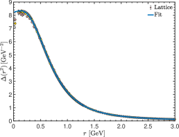
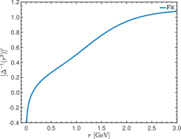
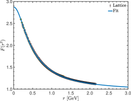
Figure 12: Left: Lattice data of Bogolubsky et al. (2009); Aguilar et al. (2021c) (points), and the fit of Eq. (105) (blue solid line), for the gluon propagator, $\Delta(r^{2})$. Center: The derivative $[\Delta^{-1}(r^{2})]^{\prime}$, obtained through differentiation of Eq. (105). Right: Lattice data (points) of Boucaud et al. (2018), and the fit of Eq. (100) (blue solid), for the ghost dressing function, $F(r^{2})$.

The fitting parameters resulting for $\Delta(r^{2})$, $F(r^{2})$, and $\mathit{L}_{{sg}}(r^{2})$ are given in Table 1 and its caption. The resulting curves for $\Delta(r^{2})$ and $F(r^{2})$ are compared to the lattice data of Bogolubsky et al. (2009); Aguilar et al. (2021c) in Fig. 12, where we also show $[\Delta^{-1}(r^{2})]^{\prime}$. The lattice data of Aguilar et al. (2021a) and corresponding fit for $\mathit{L}_{{sg}}(r^{2})$ are shown as the points and black continuous curve, respectively, in the right panel of Fig. 6.

Comparing the curve of $\mathit{L}_{{sg}}(r^{2})$ in Fig. 6 to that of $[\Delta^{-1}(r^{2})]^{\prime}$ in Fig. 12, we see that $[\Delta^{-1}(r^{2})]^{\prime}$ is responsible for reproducing the overall shape of $\mathit{L}_{{sg}}(r^{2})$ in the WI of Eq. (58), with the other ingredients providing minor quantitative modulations.

Now, it is clear from Figs. 6 and 12 that the lattice quantity with the largest error in the present analysis is $\mathit{L}_{{sg}}(r^{2})$. In order to propagate the error of $\mathit{L}_{{sg}}(r^{2})$ to other quantities that depend on it, we make a band around $\mathit{L}_{{sg}}(r^{2})$, delimited by

$$\mathit{L}_{{sg}}^{\pm}(r^{2})=\mathit{L}_{{sg}}(r^{2})\pm\frac{\delta_{1}}{1+(r^{2}/\delta_{2}^{2})^{2}}\,,$$ (107)

with parameters $\delta_{1}=0.08$ and $\delta_{2}^{2}=5$ GeV².

	$\kappa^{2}$ [GeV2]	$\eta_{1}^{2}$ [GeV2]	$\eta_{2}^{2}$ [GeV2]	$b_{0}$	$b_{1}^{2}$ [GeV-2]	$b_{2}^{2}$ [GeV2]	$b_{3}^{2}$ [GeV2]
$F(r^{2})$	-	3.60	0.148	-0.566	0.004	0.375	24.2
$\Delta(r^{2})$	1.33	0.889	2.570	1.254	0.723	1.553	2.08
$\mathit{L}_{{sg}}(r^{2})$	18.2	0.200	6.36	0.241	-0.646	0.310	1.28

Table 1: Fitting parameters $\kappa^{2}$, $\eta^{2}_{i}$, $b_{0}$, and $b^{2}_{i}$, to be used in each of Eqs.  (100),  (105), and (106) for $F(r^{2})$, $\Delta(r^{2})$, and $\mathit{L}_{{sg}}(r^{2})$, respectively. In addition to the values below, we set $d=0.075$ and $\ell=0.11$, in Eqs. (105) and (106), respectively, and $\omega=0.214$ in the Eqs. (100), (105), and (106).

Lastly, for the value of $\alpha_{s}$ in the asymmetric MOM scheme, which appears in the SDE for ${\cal W}(r^{2})$ given by Eq. (86), we use the value $\alpha_{s}=0.27$ determined by lattice simulations Athenodorou et al. (2016); Boucaud et al. (2017). For the $F(0)$ appearing in Eq. (58) we obtain from Eq. (100) and Table 1 the value $F(0)=2.88$.

References

- Marciano and Pagels (1978) W. J. Marciano and H. Pagels, Phys. Rept. 36, 137 (1978).
- Roberts and Williams (1994) C. D. Roberts and A. G. Williams, Prog. Part. Nucl. Phys. 33, 477 (1994).
- Alkofer and von Smekal (2001) R. Alkofer and L. von Smekal, Phys. Rept. 353, 281 (2001).
- Fischer (2006) C. S. Fischer, J. Phys. G 32, R253 (2006).
- Roberts (2008) C. D. Roberts, Prog. Part. Nucl. Phys. 61, 50 (2008).
- Binosi and Papavassiliou (2009) D. Binosi and J. Papavassiliou, Phys. Rept. 479, 1 (2009).
- Binosi et al. (2015) D. Binosi, L. Chang, J. Papavassiliou, and C. D. Roberts, Phys. Lett. B742, 183 (2015).
- Cloet and Roberts (2014) I. C. Cloet and C. D. Roberts, Prog. Part. Nucl. Phys. 77, 1 (2014).
- Aguilar et al. (2016a) A. C. Aguilar, D. Binosi, and J. Papavassiliou, Front. Phys.(Beijing) 11, 111203 (2016a).
- Binosi et al. (2016) D. Binosi, L. Chang, J. Papavassiliou, S.-X. Qin, and C. D. Roberts, Phys. Rev. D93, 096010 (2016).
- Binosi et al. (2017) D. Binosi, C. Mezrag, J. Papavassiliou, C. D. Roberts, and J. Rodriguez-Quintero, Phys. Rev. D96, 054026 (2017).
- Huber (2020) M. Q. Huber, Phys. Rept. 879, 1 (2020).
- Pawlowski et al. (2004) J. M. Pawlowski, D. F. Litim, S. Nedelko, and L. von Smekal, Phys. Rev. Lett. 93, 152002 (2004).
- Pawlowski (2007) J. M. Pawlowski, Annals Phys. 322, 2831 (2007).
- Cyrol et al. (2018a) A. K. Cyrol, M. Mitter, J. M. Pawlowski, and N. Strodthoff, Phys. Rev. D97, 054006 (2018a).
- Corell et al. (2018) L. Corell, A. K. Cyrol, M. Mitter, J. M. Pawlowski, and N. Strodthoff, SciPost Phys. 5, 066 (2018).
- Blaizot et al. (2021) J.-P. Blaizot, J. M. Pawlowski, and U. Reinosa, Annals Phys. 431, 168549 (2021).
- Cucchieri and Mendes (2007) A. Cucchieri and T. Mendes, PoS LATTICE2007, 297 (2007).
- Cucchieri and Mendes (2008) A. Cucchieri and T. Mendes, Phys. Rev. Lett. 100, 241601 (2008).
- Cucchieri and Mendes (2010) A. Cucchieri and T. Mendes, Phys. Rev. D81, 016005 (2010).
- Bogolubsky et al. (2007) I. Bogolubsky, E. Ilgenfritz, M. Muller-Preussker, and A. Sternbeck, PoS LATTICE2007, 290 (2007).
- Bogolubsky et al. (2009) I. Bogolubsky, E. Ilgenfritz, M. Muller-Preussker, and A. Sternbeck, Phys. Lett. B676, 69 (2009).
- Oliveira and Silva (2009) O. Oliveira and P. Silva, PoS LAT2009, 226 (2009).
- Oliveira and Bicudo (2011) O. Oliveira and P. Bicudo, J. Phys. G G38, 045003 (2011).
- Maas (2013) A. Maas, Phys. Rept. 524, 203 (2013).
- Boucaud et al. (2012) P. Boucaud, J. P. Leroy, A. L. Yaouanc, J. Micheli, O. Pene, and J. Rodríguez-Quintero, Few Body Syst. 53, 387 (2012).
- Oliveira and Silva (2012) O. Oliveira and P. J. Silva, Phys. Rev. D86, 114513 (2012).
- Maris and Roberts (1997) P. Maris and C. D. Roberts, Phys. Rev. C 56, 3369 (1997).
- Maris and Roberts (2003) P. Maris and C. D. Roberts, Int. J. Mod. Phys. E12, 297 (2003).
- Braun et al. (2010) J. Braun, H. Gies, and J. M. Pawlowski, Phys. Lett. B684, 262 (2010).
- Eichmann et al. (2009) G. Eichmann, I. C. Cloet, R. Alkofer, A. Krassnigg, and C. D. Roberts, Phys. Rev. C79, 012202 (2009).
- Cloet et al. (2009) I. Cloet, G. Eichmann, B. El-Bennich, T. Klahn, and C. Roberts, Few Body Syst. 46, 1 (2009).
- Boucaud et al. (2008) P. Boucaud, J. Leroy, L. Y. A., J. Micheli, O. Pène, and J. Rodríguez-Quintero, J. High Energy Phys. 06, 099 (2008).
- Eichmann et al. (2010) G. Eichmann, R. Alkofer, A. Krassnigg, and D. Nicmorus, Phys. Rev. Lett. 104, 201601 (2010).
- Fister and Pawlowski (2013) L. Fister and J. M. Pawlowski, Phys. Rev. D88, 045010 (2013).
- Meyer and Swanson (2015) C. A. Meyer and E. S. Swanson, Prog. Part. Nucl. Phys. 82, 21 (2015).
- Eichmann et al. (2016) G. Eichmann, H. Sanchis-Alepuz, R. Williams, R. Alkofer, and C. S. Fischer, Prog. Part. Nucl. Phys. 91, 1 (2016).
- Sanchis-Alepuz et al. (2018) H. Sanchis-Alepuz, R. Alkofer, and C. S. Fischer, Eur. Phys. J. A 54, 41 (2018).
- Alkofer et al. (2019) R. Alkofer, A. Maas, W. A. Mian, M. Mitter, J. París-López, J. M. Pawlowski, and N. Wink, Phys. Rev. D 99, 054029 (2019).
- Gao et al. (2018) F. Gao, S.-X. Qin, C. D. Roberts, and J. Rodríguez-Quintero, Phys. Rev. D97, 034010 (2018).
- Souza et al. (2020) E. V. Souza, M. N. Ferreira, A. C. Aguilar, J. Papavassiliou, C. D. Roberts, and S.-S. Xu, Eur. Phys. J. A 56, 25 (2020).
- Xu et al. (2019) S.-S. Xu, Z.-F. Cui, L. Chang, J. Papavassiliou, C. D. Roberts, and H.-S. Zong, Eur. Phys. J. A55, 113 (2019).
- Aguilar et al. (2019a) A. C. Aguilar et al., Eur. Phys. J. A 55, 190 (2019a).
- Huber et al. (2020) M. Q. Huber, C. S. Fischer, and H. Sanchis-Alepuz, Eur. Phys. J. C 80, 1077 (2020).
- Roberts and Schmidt (2020) C. D. Roberts and S. M. Schmidt, Eur. Phys. J. ST 229, 3319 (2020).
- Roberts (2020) C. D. Roberts, Symmetry 12, 1468 (2020).
- Horak et al. (2021) J. Horak, J. Papavassiliou, J. M. Pawlowski, and N. Wink, Phys. Rev. D 104, 074017 (2021).
- Roberts (2021) C. D. Roberts, [arXiv:2101.08340 [hep-ph]] .
- Smit (1974) J. Smit, Phys. Rev. D 10, 2473 (1974).
- Cornwall (1982) J. M. Cornwall, Phys. Rev. D 26, 1453 (1982).
- Bernard (1982) C. W. Bernard, Phys. Lett. B 108, 431 (1982).
- Bernard (1983) C. W. Bernard, Nucl. Phys. B 219, 341 (1983).
- Donoghue (1984) J. F. Donoghue, Phys. Rev. D 29, 2559 (1984).
- Mandula and Ogilvie (1987) J. Mandula and M. Ogilvie, Phys. Lett. B 185, 127 (1987).
- Cornwall and Papavassiliou (1989) J. M. Cornwall and J. Papavassiliou, Phys. Rev. D 40, 3474 (1989).
- Wilson et al. (1994) K. G. Wilson, T. S. Walhout, A. Harindranath, W.-M. Zhang, R. J. Perry, and S. D. Glazek, Phys. Rev. D49, 6720 (1994).
- Philipsen (2002) O. Philipsen, Nucl. Phys. B628, 167 (2002).
- Aguilar et al. (2003) A. C. Aguilar, A. A. Natale, and P. S. Rodrigues da Silva, Phys. Rev. Lett. 90, 152001 (2003).
- Aguilar and Natale (2004) A. C. Aguilar and A. A. Natale, J. High Energy Phys. 08, 057 (2004).
- Aguilar and Papavassiliou (2006) A. C. Aguilar and J. Papavassiliou, J. High Energy Phys. 12, 012 (2006).
- Aguilar et al. (2008) A. C. Aguilar, D. Binosi, and J. Papavassiliou, Phys. Rev. D78, 025010 (2008).
- Fischer et al. (2009) C. S. Fischer, A. Maas, and J. M. Pawlowski, Annals Phys. 324, 2408 (2009).
- Tissier and Wschebor (2010) M. Tissier and N. Wschebor, Phys. Rev. D 82, 101701 (2010).
- Binosi et al. (2012) D. Binosi, D. Ibañez, and J. Papavassiliou, Phys. Rev. D86, 085033 (2012).
- Serreau and Tissier (2012) J. Serreau and M. Tissier, Phys. Lett. B712, 97 (2012).
- Peláez et al. (2014) M. Peláez, M. Tissier, and N. Wschebor, Phys. Rev. D 90, 065031 (2014).
- Aguilar et al. (2016b) A. C. Aguilar, D. Binosi, C. T. Figueiredo, and J. Papavassiliou, Phys. Rev. D94, 045002 (2016b).
- Dudal et al. (2008) D. Dudal, J. A. Gracey, S. P. Sorella, N. Vandersickel, and H. Verschelde, Phys. Rev. D78, 065047 (2008).
- Rodríguez-Quintero (2011) J. Rodríguez-Quintero, J. High Energy Phys. 01, 105 (2011).
- Pennington and Wilson (2011) M. Pennington and D. Wilson, Phys. Rev. D84, 119901 (2011).
- Meyers and Swanson (2014) J. Meyers and E. S. Swanson, Phys. Rev. D90, 045037 (2014).
- Siringo (2016) F. Siringo, Nucl. Phys. B907, 572 (2016).
- Cyrol et al. (2018b) A. K. Cyrol, J. M. Pawlowski, A. Rothkopf, and N. Wink, SciPost Phys. 5, 065 (2018b).
- Cucchieri et al. (2009) A. Cucchieri, T. Mendes, and E. M. Santos, Phys. Rev. Lett. 103, 141602 (2009).
- Cucchieri et al. (2010) A. Cucchieri, T. Mendes, G. M. Nakamura, and E. M. Santos, PoS FACESQCD, 026 (2010).
- Bicudo et al. (2015) P. Bicudo, D. Binosi, N. Cardoso, O. Oliveira, and P. J. Silva, Phys. Rev. D92, 114514 (2015).
- Epple et al. (2008) D. Epple, H. Reinhardt, W. Schleifenbaum, and A. Szczepaniak, Phys. Rev. D77, 085007 (2008).
- Campagnari and Reinhardt (2010) D. R. Campagnari and H. Reinhardt, Phys. Rev. D82, 105021 (2010).
- Aguilar et al. (2017) A. C. Aguilar, D. Binosi, and J. Papavassiliou, Phys. Rev. D95, 034017 (2017).
- Glazek et al. (2017) S. D. Glazek, M. Gómez-Rocha, J. More, and K. Serafin, Phys. Lett. B773, 172 (2017).
- Bowman et al. (2007) P. O. Bowman, U. M. Heller, D. B. Leinweber, M. B. Parappilly, A. Sternbeck, L. von Smekal, A. G. Williams, and J.-b. Zhang, Phys. Rev. D 76, 094505 (2007).
- Kamleh et al. (2007) W. Kamleh, P. O. Bowman, D. B. Leinweber, A. G. Williams, and J. Zhang, Phys. Rev. D76, 094501 (2007).
- Ayala et al. (2012) A. Ayala, A. Bashir, D. Binosi, M. Cristoforetti, and J. Rodríguez-Quintero, Phys. Rev. D86, 074512 (2012).
- Aguilar et al. (2013) A. C. Aguilar, D. Binosi, and J. Papavassiliou, Phys. Rev. D88, 074010 (2013).
- Aguilar et al. (2020a) A. C. Aguilar, F. De Soto, M. N. Ferreira, J. Papavassiliou, J. Rodríguez-Quintero, and S. Zafeiropoulos, Eur. Phys. J. C80, 154 (2020a).
- Schwinger (1962a) J. S. Schwinger, Phys. Rev. 125, 397 (1962a).
- Schwinger (1962b) J. S. Schwinger, Phys. Rev. 128, 2425 (1962b).
- Jackiw and Johnson (1973) R. Jackiw and K. Johnson, Phys. Rev. D 8, 2386 (1973).
- Eichten and Feinberg (1974) E. Eichten and F. Feinberg, Phys. Rev. D 10, 3254 (1974).
- Aguilar et al. (2012) A. C. Aguilar, D. Ibañez, V. Mathieu, and J. Papavassiliou, Phys. Rev. D85, 014018 (2012).
- Ibañez and Papavassiliou (2013) D. Ibañez and J. Papavassiliou, Phys. Rev. D87, 034008 (2013).
- Binosi and Papavassiliou (2018) D. Binosi and J. Papavassiliou, Phys. Rev. D97, 054029 (2018).
- Aguilar et al. (2018) A. C. Aguilar, D. Binosi, C. T. Figueiredo, and J. Papavassiliou, Eur. Phys. J. C78, 181 (2018).
- Eichmann et al. (2021) G. Eichmann, J. M. Pawlowski, and J. M. Silva, arXiv:2107.05352 [hep-ph]] .
- Taylor (1971) J. Taylor, Nucl. Phys. B 33, 436 (1971).
- Slavnov (1972) A. Slavnov, Theor. Math. Phys. 10, 99 (1972).
- Cornwall and Norton (1973) J. Cornwall and R. Norton, Phys. Rev. D 8, 3338 (1973).
- Poggio et al. (1975) E. C. Poggio, E. Tomboulis, and S. H. H. Tye, Phys. Rev. D11, 2839 (1975).
- Cucchieri et al. (2006) A. Cucchieri, A. Maas, and T. Mendes, Phys. Rev. D74, 014503 (2006).
- Cucchieri et al. (2008) A. Cucchieri, A. Maas, and T. Mendes, Phys. Rev. D77, 094510 (2008).
- Athenodorou et al. (2016) A. Athenodorou, D. Binosi, P. Boucaud, F. De Soto, J. Papavassiliou, J. Rodríguez-Quintero, and S. Zafeiropoulos, Phys. Lett. B761, 444 (2016).
- Duarte et al. (2016) A. G. Duarte, O. Oliveira, and P. J. Silva, Phys. Rev. D94, 074502 (2016).
- Boucaud et al. (2018) P. Boucaud, F. De Soto, K. Raya, J. Rodríguez-Quintero, and S. Zafeiropoulos, Phys. Rev. D98, 114515 (2018).
- Boucaud et al. (2003) P. Boucaud, F. De Soto, A. Le Yaouanc, J. P. Leroy, J. Micheli, H. Moutarde, O. Pene, and J. Rodríguez-Quintero, JHEP 04, 005 (2003).
- Boucaud et al. (2004) P. Boucaud, F. De Soto, A. Le Yaouanc, J. P. Leroy, J. Micheli, O. Pene, and J. Rodríguez-Quintero, Phys. Rev. D 70, 114503 (2004).
- Aguilar et al. (2021a) A. C. Aguilar, F. De Soto, M. N. Ferreira, J. Papavassiliou, and J. Rodríguez-Quintero, Phys. Lett. B 818, 136352 (2021a).
- Aguilar et al. (2020b) A. C. Aguilar, M. N. Ferreira, and J. Papavassiliou, Eur. Phys. J. C 80, 887 (2020b).
- Aguilar et al. (2021b) A. C. Aguilar, M. N. Ferreira, and J. Papavassiliou, Eur. Phys. J. C 81, 54 (2021b).
- DeWitt (1967) B. S. DeWitt, Phys. Rev. 162, 1195 (1967).
- Honerkamp (1972) J. Honerkamp, Nucl. Phys. B 48, 269 (1972).
- ’t Hooft (1971) G. ’t Hooft, Nucl. Phys. B 35, 167 (1971).
- Kallosh (1974) R. E. Kallosh, Nucl. Phys. B 78, 293 (1974).
- Kluberg-Stern and Zuber (1975) H. Kluberg-Stern and J. B. Zuber, Phys. Rev. D 12, 482 (1975).
- Abbott (1981) L. Abbott, Nucl. Phys. B 185, 189 (1981).
- Shore (1981) G. M. Shore, Annals Phys. 137, 262 (1981).
- Abbott et al. (1983) L. F. Abbott, M. T. Grisaru, and R. K. Schaefer, Nucl. Phys. B 229, 372 (1983).
- Aguilar et al. (2014) A. C. Aguilar, D. Binosi, D. Ibañez, and J. Papavassiliou, Phys. Rev. D89, 085008 (2014).
- Becchi et al. (1976) C. Becchi, A. Rouet, and R. Stora, Annals Phys. 98, 287 (1976).
- Tyutin (1975) I. V. Tyutin, LEBEDEV-75-39 (1975).
- Papavassiliou (1990) J. Papavassiliou, Phys. Rev. D 41, 3179 (1990).
- Alkofer and Alkofer (2011) N. Alkofer and R. Alkofer, Phys. Lett. B 702, 158 (2011).
- Capri et al. (2015) M. A. L. Capri, D. Dudal, D. Fiorentini, M. S. Guimaraes, I. F. Justo, A. D. Pereira, B. W. Mintz, L. F. Palhares, R. F. Sobreiro, and S. P. Sorella, Phys. Rev. D 92, 045039 (2015).
- Pilaftsis (1997) A. Pilaftsis, Nucl. Phys. B 487, 467 (1997).
- Binosi and Papavassiliou (2008) D. Binosi and J. Papavassiliou, Phys. Rev. D77, 061702 (2008).
- Aguilar and Papavassiliou (2010) A. C. Aguilar and J. Papavassiliou, Phys. Rev. D81, 034003 (2010).
- Binosi and Papavassiliou (2002) D. Binosi and J. Papavassiliou, Phys. Rev. D66, 025024 (2002).
- Aguilar et al. (2019b) A. C. Aguilar, M. N. Ferreira, C. T. Figueiredo, and J. Papavassiliou, Phys. Rev. D99, 034026 (2019b).
- Aguilar et al. (2021c) A. C. Aguilar, C. O. Ambrósio, F. De Soto, M. N. Ferreira, B. M. Oliveira, J. Papavassiliou, and J. Rodríguez-Quintero, Phys. Rev. D 104, 054028 (2021c).
- Parrinello (1994) C. Parrinello, Phys. Rev. D50, R4247 (1994).
- Alles et al. (1997) B. Alles, D. Henty, H. Panagopoulos, C. Parrinello, C. Pittori, and D. G. Richards, Nucl. Phys. B502, 325 (1997).
- Parrinello et al. (1998) C. Parrinello, D. Richards, B. Alles, H. Panagopoulos, and C. Pittori (UKQCD), Nucl. Phys. B Proc. Suppl. 63, 245 (1998).
- Boucaud et al. (1998) P. Boucaud, J. P. Leroy, J. Micheli, O. Pene, and C. Roiesnel, J. High Energy Phys. 10, 017 (1998).
- Sternbeck et al. (2017) A. Sternbeck, P.-H. Balduf, A. Kizilersu, O. Oliveira, P. J. Silva, J.-I. Skullerud, and A. G. Williams, PoS LATTICE2016, 349 (2017).
- Vujinovic and Mendes (2019) M. Vujinovic and T. Mendes, Phys. Rev. D99, 034501 (2019).
- Williams et al. (2016) R. Williams, C. S. Fischer, and W. Heupel, Phys. Rev. D93, 034026 (2016).
- Nakanishi (1969) N. Nakanishi, Prog. Theor. Phys. Suppl. 43, 1 (1969).
- Blank and Krassnigg (2011) M. Blank and A. Krassnigg, Comput. Phys. Commun. 182, 1391 (2011).
- Ball and Chiu (1980) J. S. Ball and T.-W. Chiu, Phys. Rev. D 22, 2550 (1980), [Erratum: Phys.Rev.D 23, 3085 (1981)].
- Aguilar et al. (2019c) A. C. Aguilar, M. N. Ferreira, C. T. Figueiredo, and J. Papavassiliou, Phys. Rev. D99, 094010 (2019c).
- Huber (2017) M. Q. Huber, Eur. Phys. J. C77, 733 (2017).
- Boucaud et al. (2017) P. Boucaud, F. De Soto, J. Rodríguez-Quintero, and S. Zafeiropoulos, Phys. Rev. D95, 114503 (2017).