The range of a self-similar additive gamma process is a scale invariant Poisson point process

Abstract

It is shown that for a non-decreasing self-similar stochastic process $T$ with independent increments, the range of $T$ forms a Poisson point process with $\sigma$-finite intensity if and only if the one-dimensional distribution of $T(1)$ is of the gamma type. This follows from a general hold-jump description of such processes $T$, and implies the known result that the spacings between consecutive points of a scale invariant Poisson point process, with intensity $\theta x^{-1}dx$, are the points of another scale invariant Poisson point process with the same intensity.

Key words

scale invariant Poisson spacings, Poisson point processes, self-similar processes, Sato processes, range, records, extremal processes

1 Introduction

A point process $N_{X}(B)=\#\{z\in{\mathbb{Z}}:X_{z}\in B\}$, counting numbers of points in subintervals $B$ of the positive half line ${\mathbb{R}}_{+}:=(0,\infty)$, for some indexing of these points $X_{z}$ by $z$ in the set of integers ${\mathbb{Z}}$, is called scale invariant if for each $c>0$ the point process $N_{cX}$, counting the scaled points $\{cX_{z}:z\in{\mathbb{Z}}\}$, has the same finite-dimensional distributions as $N_{X}$, as $B$ varies over subintervals of ${\mathbb{R}}_{+}$. Assuming the point process $N_{X}$ is simple, meaning the points $X_{z}$ are all distinct, the point process $N_{X}$ is then regarded as encoding the random countable set

$$range(X_{z},\in{\mathbb{Z}}):=\{X_{z},\in{\mathbb{Z}}\}.$$ (1.1)

So the identity in distribution of simple point processes $N_{X}$ and $N_{cX}$ may be indicated by the notation

$$range(X_{z},z\in{\mathbb{Z}})\stackrel{{\scriptstyle d}}{{=}}range(cX_{z},z\in{\mathbb{Z}}).$$ (1.2)

It is well known that a Poisson point process (PPP) on ${\mathbb{R}}_{+}$ is scale invariant if and only if its intensity measure is $\theta x^{-1}dx$ for some $\theta\geq 0$, when the process is called a $PPP(\theta x^{-1}dx)$, or a scale invariant Poisson point process with rate $\theta$. So the parameter $\theta$ is the intensity of such a point process relative to the scale invariant measure $x^{-1}dx$ on the positive half-line, and for $0<a<b<\infty$, the number of points in $(a,b)$ has a Poisson distribution with mean $\theta\log(b/a)$.

The following result on scale invariant Poisson spacings arises in various contexts. The case $\theta=1$ is contained in the theory of records and extremal processes, first developed by Dwass [7, 8, 9] and further studied by Resnick and Rubinovitch [31], and Shorrock [35]. The formulation for general $\theta>0$ is due to Arratia [1, 2], who sketched a proof which was later detailed by Arratia, Barbour and Tavaré [3, Section 7].

Theorem 1.1 (Scale invariant Poisson spacings)

Fix $\theta>0$. Let $(T_{z},z\in{\mathbb{Z}})$, with $T_{z}<T_{z+1}$ for all $z\in{\mathbb{Z}}$, be an exhaustive listing of the points of a scale invariant PPP with rate $\theta$. Then

$$range(T_{z+1}-T_{z},z\in{\mathbb{Z}})\stackrel{{\scriptstyle d}}{{=}}range(T_{z},z\in{\mathbb{Z}}).$$ (1.3)

Less formally, the theorem states:

• the spacings between consecutive points of a scale invariant Poisson point process on the positive half-line are the points of another scale invariant Poisson point process with the same rate.

This article places Theorem 1.1 in the broader context of stochastic processes $T=(T(s),s>0)$ which are self-similar additive (SSA), meaning that

• $T$ is self-similar: for all $c>0$,

  $$(T({cs}),s>0)\stackrel{{\scriptstyle d}}{{=}}(cT(s),s>0);$$ (1.4)

• $T$ is additive: meaning $T$ has independent increments, and $T$ is stochastically continuous with càdlàg paths starting at $0$

  $$\lim_{s\to 0+}T(s)=0.$$ (1.5)

Such a process $T$ is also called

• a process of class $L$ [32], as the distribution of $T(1)$ is of class $L$, a subclass of infinitely divisible laws studied by Lévy [25], or

• or a Sato process [5], and these processes were studied in depth by Sato [32, 33].

Here we focus on $range(T)$, the set of all values ever visited by $T$, regarded as a random subset of ${\mathbb{R}}_{+}$, for a non-negative, hence non-decreasing SSA process $T$ with no drift component. As recalled in Section 3, it is known that for such an SSA process $T$, the Lévy-Khinchine representation of the Laplace transform of $T(1)$ has the special form

$$\log{\mathbb{E}}e^{-uT(1)}=\int_{0}^{\infty}\left(e^{-ux}-1\right)\frac{k(x)}{x}dx,$$ (1.6)

for a uniquely determined right continuous non-increasing key function $k:{\mathbb{R}}_{+}\to{\mathbb{R}}_{+}$ subject to

$$\int_{0}^{\infty}(x\wedge 1)\frac{k(x)}{x}dx<\infty.$$ (1.7)

So the Lévy measure of $T(1)$ has a density relative to Lebesgue measure $dx$ of the form $k(x)/x$ for such a key function $k(x)$.

Consider now the random countable set of jump times of $T$:

$$\{s>0:T(s)>T(s-)\}.$$ (1.8)

Let $k(0+):=\lim_{x\to 0+}k(x)$. It follows easily from self-similarity of $T$ that

• either $k(0+)=\infty$ and the set of jump times is dense in ${\mathbb{R}}_{+}$;

• or $k(0+)<\infty$ and the jump times are the points of a scale invariant PPP with rate $\theta=k(0+)$, when we say the SSA process $T$ has (finite) rate $\theta$.

The identification of the rate $\theta=k(0+)$ is part of an explicit hold-jump construction of $T$ with finite rate, provided later in Theorem 4.1. Taking the jump sizes into consideration, as well as the jump times, the Lévy-Itô representation of jumps, discussed in Section 4, shows that the random countable set of ordered pairs of jump times and jump sizes

$$\{(s,T(s)-T(s-)):s>0,T(s)>T(s-)\}$$ (1.9)

is the set of points of a scale invariant Poisson point process on ${\mathbb{R}}_{+}^{2}$. This leads to the following theorem:

Theorem 1.2

For a SSA non-decreasing process $T$, with no drift component and key function $k(x)$, if $k(0+)=\theta$ is finite, then

• $range(T):=\{T(s):s>0\}$ is a scale invariant point process on ${\mathbb{R}}_{+}$ with rate $\theta$;

• the set of jump times of $T$ is a scale invariant PPP on ${\mathbb{R}}_{+}$ with rate $\theta$;

• the set of jump sizes of $T$ is a scale invariant PPP on ${\mathbb{R}}_{+}$ with rate $\theta$.

Here, (II) and (III) are just two coordinate projections of the self-similar Poisson point process (1.9) in the positive quadrant. Note that in (I) it is not asserted that $range(T)$ is Poisson point process, only that this point process is scale-invariant with mean intensity measure $\theta x^{-1}dx$. Beyond that, we know rather little about attributes of $range(T)$ as a point process on ${\mathbb{R}}_{+}$, such as its higher order factorial moments or Janossy measures, except in the special case when $T(1)$ is gamma distributed, and range$(T)$ turns out to be Poissonian.

To provide a more detailed description of the range of a non-decreasing SSA process $T$ with finite rate, let the scale invariant PPP of jump times of $T$ be indexed by ${\mathbb{Z}}$ in an increasing way, say

$$0<\cdots<S_{-1}<S_{0}<S_{1}<\cdots<\infty,$$ (1.10)

and define for each $z\in{\mathbb{Z}}$

$$T_{z}:=T(S_{z}).$$ (1.11)

So the jump of $T$ at time $s=S_{z}$ is from $T_{z-1}=T(S_{z}-)$ to $T_{z}=T(S_{z})$. See Figure 1 for an illustration. Then the random countable range of $T$ is

$$range(T(s),s>0)=range(T_{z},z\in{\mathbb{Z}})$$ (1.12)

so the points in the range of $T$ are also indexed by ${\mathbb{Z}}$ in increasing order

$$0<\cdots<T_{-1}<T_{0}<T_{1}<\cdots<\infty,$$ (1.13)

as in the setup in for scale-invariant Poisson spacings in Theorem 1.1.

Here we are not specific about how $S_{0}$ is selected from the random set of jump times of $T$, since the choice is not important when considering the simple point process $\{(T_{z},T_{z+1}-T_{z}):z\in{\mathbb{Z}}\}$ as a random set on ${\mathbb{R}}_{+}^{2}$. It will be more convenient to define $S_{0}$ either so that $S_{0}\leq 1<S_{1}$ or so that $T_{0}\leq 1<T_{1}$.

Thus for a scale-invariant point process constructed as the range of a non-decreasing SSA process $T$ with finite rate $\theta$, comparing the point process of spacings between points, as on the left side of (1.3), and the points themselves on the right side of (1.3),

• the spacings between points are the jump sizes of $T$:

  $$range(T_{z+1}-T_{z},z\in{\mathbb{Z}})=range(T(s)-T({s-})>0:s>0)$$ (1.14)

  which forms a scale invariant PPP with rate $\theta$, no matter what the key function $k(x)$ of $T$ with $k(0+)=\theta$;

• the points themselves form the range of $T$:

  $$range(T_{z},z\in{\mathbb{Z}})=range(T(s),s>0)$$ (1.15)

  which is a scale invariant point process with rate $\theta$, which might or might not be Poissonian, depending on the choice of the key function.

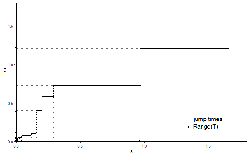
Figure 1: An SSA gamma process $(T(s),s>0)$, its range, and jump times

So to establish the spacings theorem 1.1, for a scale-invariant Poisson process with rate $\theta$, it only remains to show that for a suitable choice of the key function $k(x)$ with $k(0+)=\theta$, the range of $T$ is in fact Poissonian. That scale-invariant Poisson feature of range$(T)$, with rate $\theta=1$, was established by Dwass in the 1960s for the SSA exponential process $T$, with $k(x)=e^{-\lambda x}$ for some $\lambda>0$, so $T(1)\sim$ gamma$(1,\lambda)$ (or exp$(\lambda)$) has the exponential distribution with rate $\lambda$, with tail probability

$${\mathbb{P}}(T(1)>x)=e^{-\lambda x}1(x>0).$$ (1.16)

Our main point here is that the Poisson spacings theorem for a general rate $\theta>0$ is a similar consequence of the following result, which we establish in Sections 5 and 6:

Theorem 1.3

Fix $\theta>0$. For an SSA process $T:=(T(s),s>0)$,

• range$(T)$ is a scale invariant PPP on ${\mathbb{R}}_{+}$ with rate $\theta$,

if and only if

• the distribution of $T(1)$ is gamma$(\theta,\lambda)$ for some $\lambda>0$, with probability density

  $$\frac{d}{dx}{\mathbb{P}}(T(1)\leq x)=\frac{\lambda^{\theta}}{\Gamma(\theta)}x^{\theta-1}e^{-\lambda x}1(x>0).$$ (1.17)

Implicit in this result is a well known consequence of the Lévy-Khinchine formula:

$$\mbox{ \em the gamma$(\theta,\lambda)$ distribution of $T(1)$ has key function $k(x)=\theta e^{-\lambda x}$}.$$ (1.18)

However, some effort is required to pass from this fact to either of the implications of Theorem 1.3.

The rest of this article is organized as follows:

• Section 2 collects for later use some easy results about a scale invariant PPP.

• Section 3 recalls basic facts about SSA processes and selfdecomposable laws.

• Section 4 characterizes an SSA non-decreasing process $T$ with finite rate by its generic jump distribution, which can be read from the key function in the Lévy-Khinchine representation. The corresponding hold-jump description of $T$ is the basis of proofs in Section 5.

• Section 5 offers proves the “if” part of Theorem 1.3, that the range of an SSA gamma process is a PPP, in two different ways, based on the hold-jump description provided in Section 4.

• Section 6 provides a general uniqueness theorem which includes the converse of Theorem 1.3: under a technical condition, the distribution of the range of a SSA non-decreasing process uniquely determines the distribution of the process itself, up to a scale factor.

• Section 7 briefly discusses three different processes associated with a selfdecomposable law, then introduces a two-parameter process which provides a coupling of SSA processes with stationary independent increments in a second parameter.

• Section 8 offers some historical notes, including how the case $\theta=1$ of Theorem 1.1 arises in the theory of extremal processes, and how the general case $\theta>0$ is related to the Ewens sampling formula.

2 Scale invariant point processes

If a point process $X:=\{X_{z},z\in{\mathbb{Z}}\}$ on ${\mathbb{R}}_{+}$ is scale invariant, i.e.

$$range(X)\stackrel{{\scriptstyle d}}{{=}}range(cX),\qquad\forall c>0,$$ (2.1)

then $X$ is a simple point process with intensity measure $\theta x^{-1}dx$ for some $\theta$, with $0<\theta\leq\infty$. Then we say $X$ is a scale invariant point process on ${\mathbb{R}}_{+}$ with rate $\theta$. We observe that

• the inversion $1/X:=\{1/X_{z},z\in{\mathbb{Z}}\}$ of a scale invariant point process $X$ on ${\mathbb{R}}_{+}$ is a scale invariant point process on ${\mathbb{R}}_{+}$ with the same rate.

By considering $L:=\log X$, this corresponds to a well known fact about stationary point processes on ${\mathbb{R}}$. Just as not all stationary point processes on the line are reversible, not all scale invariant point process are invariant under inversion. However, the distribution of a Poisson point process is entirely determined by its intensity measure, hence:

• if $X:=\{X_{z},z\in{\mathbb{Z}}\}$ is a scale invariant PPP then

  $$range(1/X)\stackrel{{\scriptstyle d}}{{=}}range(X).$$ (2.2)

The following lemma provides some useful characterizations of a scale invariant PPP. Recall that for $U$ with uniform distribution on $[0,1]$, and $\theta>0$, the distribution of $U^{1/\theta}$ is the beta$(\theta,1)$ distribution on $[0,1]$ with probability density

$$\frac{d}{du}{\mathbb{P}}(U^{1/\theta}\leq u)=\theta u^{\theta-1}1(0<u<1).$$ (2.3)

Lemma 2.1

Fix $x>0$ and $\theta>0$. Suppose a scale invariant point process $X=\{X_{z},z\in{\mathbb{Z}}\}$ is indexed in increasing manner with

$$0<\cdots<X_{-2}<X_{-1}<X_{0}\leq x<X_{1}<X_{2}<\cdots<\infty.$$ (2.4)

Then the following three conditions are equivalent:

• $X$ is a scale invariant PPP with rate $\theta$;

• $x/X_{1}$ and $X_{z-1}/X_{z}$ for $z\geq 2$ are independent and identically distributed (i.i.d.) beta$(\theta,1)$ random variables;

• $X_{0}/x$ and $X_{z-1}/X_{z}$ for $z<0$ are i.i.d. beta$(\theta,1)$ random variables.

Proof Consider $L:=\{L_{z}=\log(X_{z}),z\in{\mathbb{Z}}\}$. Then $L$ is a stationary PPP with intensity measure $\theta d\ell$ on ${\mathbb{R}}$ if and only if $X$ is a scale invariant PPP with rate $\theta$. The statements of the lemma are just transformations of well known characterizations of a stationary PPP on the line.  

3 Selfdecomposable laws and SSA processes

This section recalls some known results about self-similar additive processes and their one-dimensional distributions, known as the selfdecomposable laws. Following Sato [32, 33], we call a process $T:=(T(s),s>0)$ self-similar with exponent $H$ if

$$(T({cs}),s>0)\stackrel{{\scriptstyle d}}{{=}}(c^{H}T(s),s>0)\qquad(c>0),$$ (3.1)

in the sense of equality of finite-dimensional distributions. If $T$ is also additive, as defined in Section 1, we say $T$ is $H$-self-similar additive ($H$-SSA). We omitted the prefix ‘$H$-’ when $H=1$ in (1.4), because it has no impact on our discussion of $range(T)$ thanks to Lemma 3.2 below.

Easily from the definition, for an $H$-SSA process $T$, the one-dimensional distribution of $T(1)$ is selfdecomposable, meaning that for each $0<a<1$, there is the equality in distribution

$$T(1)\stackrel{{\scriptstyle d}}{{=}}aT(1)+R_{a},$$ (3.2)

for some random variable $R_{a}$ independent of $T(1)$. It is known [33, Theorem 15.3] that the class of selfdecomposable laws is identical to the class $L$ introduced by Lévy [25] and Khintchine [22]. Lévy showed that such laws are infinitely divisible with a special structure of their Lévy measure. Specifically, from Sato and Yamazato [34], the Lévy-Khinchine representation of a selfdecomposable distribution of $X$ is

$${\mathbb{E}}e^{iuX}=\exp\left\{ibu-\mbox{$\frac{1}{2}$}\sigma^{2}u^{2}+\int_{{\mathbb{R}}-\{0\}}\left(e^{iux}-1-\frac{iux}{1+u^{2}}\right)\frac{k(x)}{x}dx\right\},$$ (3.3)

where $b$ is real, $\sigma^{2}\geq 0$ and $k(x)$ is both

• non-negative, non-increasing on ${\mathbb{R}}_{+}$ and non-positive, non-increasing on ${\mathbb{R}}_{-}$;

• subject to the usual requirement for a Lévy density $k(x)/x$ that

  $$\int_{{\mathbb{R}}-\{0\}}(x^{2}\wedge 1)\frac{k(x)}{x}dx<\infty.$$ (3.4)

Hence, assuming the distribution of $X$ is infinitely divisible, the distribution is selfdecomposable if and only its Lévy measure has a density of the form $k(x)/x$ where $k(x)$ satisfies condition (a) above. Sato [32] gave the following uniqueness theorem for the relationship between selfdecomposable laws and $H$-SSA processes.

Theorem 3.1

For each $H$-SSA process $(T(s),s>0)$, the marginal distribution of $T(s)$ is selfdecomposable. And for each selfdecomposable distribution $\mu$ and each $H>0$, there exists an $H$-SSA process $(T(s),s>0)$, unique in finite-dimensional distributions, such that $T(1)$ has distribution $\mu$.

We restrict the discussion to the case of $H=1$ for most of the rest of this article, thanks to the following lemma.

Lemma 3.2

Suppose $(T(s),s>0)$ is an $H$-SSA non-decreasing process. Then the time change

$$\tilde{T}(s)=T({s^{1/H}})\qquad(s>0),$$ (3.5)

gives a $1$-SSA non-decreasing process $(\tilde{T}(s),s\geq 0)$ with $range(\tilde{T})=range(T)$.

We are primarily interested in the case of a $1$-SSA process $T$ that is non-decreasing and with no drift. Then (3.3) and (3.4) reduce to the formulas (1.6) and (1.7) for the Laplace transform of $T(1)$.

So the Lévy density of $T(s)$ at $x>0$ is $k(x/s)/x$. As a result, the distribution of $T$ is fully characterized by the key function $k(x)$, as detailed further in Section 4.

4 Hold-jump description

This section presents the relationship between the rate $\theta<\infty$ and the key function $k(x)$ of a $1$-SSA non-decreasing process with finite rate $\theta$. The hold-jump description after the jump over $1$ will then be introduced as a framework to describe $range(T)\cap[1,\infty)$, as required to check whether $range(T)$ is Poisson using Lemma 2.1.

4.1 Rate and generic jump

Theorem 4.1

Suppose $T:=(T(s),s>0)$ is a $1$-SSA non-decreasing process with no drift, finite rate $\theta$ and key function $k(x)$. Then $k(0+)=\theta$ and

$$T(s)=\sum_{z\in{\mathbb{Z}}}S_{z}J_{z}1(S_{z}\leq s),\qquad(s>0)$$ (4.1)

where

• the jump times $(S_{z},z\in{\mathbb{Z}})$ are the points of a scale invariant PPP with rate $\theta$;

Assuming also that these jump times are listed in an order depending only on their point process (1.8), for instance in an increasing order with $S_{0}$ the time of the first jump after time $s=1$,

• the normalized jumps $(J_{z},z\in{\mathbb{Z}})$ form a sequence of i.i.d. copies of a positive random variable $J$, called the generic jump of $T$, with tail probability

  $${\mathbb{P}}(J>x)=\frac{k(x)}{\theta},\qquad(x\geq 0);$$ (4.2)

• the sequence of jump times $(S_{z},z\in{\mathbb{Z}})$ is independent of the sequence of normalized jumps $(J_{z},z\in{\mathbb{Z}})$.

Proof The self-similarity of $T$ ensures that there are no jumps at fixed times. Thus, as a non-decreasing additive process, $T(s)$ has the following almost surely unique Lévy-Itô representation [21, Theorem 16.3]:

$$T(s)=a_{s}+\int_{0}^{s}\int_{0}^{\infty}x\eta(dy~{}dx),\qquad(s>0).$$ (4.3)

where $a_{s}$ is a non-decreasing function with $a_{0}=0$ and $\eta(dy~{}dx)$ is a Poisson point process on $(0,\infty)^{2}$ satisfying

$$\int_{0}^{s}\int_{0}^{\infty}(x\wedge 1){\mathbb{E}}\eta(dy~{}dx)<\infty.\qquad(s>0)$$ (4.4)

In fact, $\eta$ characterizes the jump structure of $T$

$$\eta(\cdot)=\sum_{y}1\{(s,\Delta_{y})\in\cdot\}$$ (4.5)

where the summation extends over all times $y>0$ with $\Delta_{y}:=T(y)-T({y-})>0$. Hence

$$T(s)=a_{s}+\sum_{y}\Delta_{y}1(y\leq s)\qquad(s>0).$$ (4.6)

We call this $\eta$ the underlying Poisson point process of the non-decreasing SSA process $T$. Taking into account self-similarity of $T$, it is easy to see that $a_{s}\equiv a_{1}s$. If we further require $T$ to be a pure jump process, then $a_{s}\equiv 0$. Moreover, as we know the jump times are from a scale invariant PPP with rate $\theta$, the representation (4.1) follows immediately from self-similarity. To finish the proof, it remains to show (4.2).

Thanks again to self-similarity, note that $\{(S_{z},\Delta_{S_{z}}=S_{z}J_{z}),z\in{\mathbb{Z}}\}$ is an exhaustive listing of points from the underlying Poisson point process $\eta$ on ${\mathbb{R}}_{+}^{2}$ with intensity measure

$$\nu(ds~{}dy):={\mathbb{E}}\eta(ds~{}dy)=\theta s^{-1}ds~{}{\mathbb{P}}(sJ\in dy).$$ (4.7)

Hence, for each Borel set $B\subset{\mathbb{R}}_{+}$ and $a>0$,

$$\int_{0}^{a}\theta s^{-1}{\mathbb{P}}(sJ\in B)ds =\int_{y\in{\mathbb{R}}_{+}}dF_{J}(y)\int_{s\in{\mathbb{R}}_{+}}\theta s^{-1}1(sy\in B,s<a)ds$$ (4.8)

$$(\text{set }s=x/y)\qquad =\int_{y\in{\mathbb{R}}_{+}}dF_{J}(y)\int_{x\in{\mathbb{R}}_{+}}\theta x^{-1}1(x\in B,y>x/a)dx$$ (4.9)

$$=\int_{x\in B}\theta x^{-1}dx\int_{y>x/a}dF_{J}(y)$$ (4.10)

$$=\int_{x\in B}\frac{\theta~{}{\mathbb{P}}(J>x/a)}{x}dx.$$ (4.11)

But the Lévy measure of $T(1)$ is

$$\frac{k(x)}{x}dx=\int_{s\in(0,1]}\theta s^{-1}{\mathbb{P}}(sJ\in dx)ds,$$ (4.12)

which implies (4.2) by setting $a=1$ in (4.11).

 

To illustrate Theorem 4.1, we give two examples.

Example 4.2

Fix $\theta,\lambda>0$. A $1$-SSA gamma process $(T(s),s>0)$ with $T(1)\sim$ gamma$(\theta,\lambda)$ has exponential generic jump $J\sim$ exp$(\lambda)$ and finite rate $\theta$, thanks to the key function given in (1.18).

Example 4.3

This example is implicit in the discussion of the least concave majorant of a one-dimensional Brownian motion by Groeneboom [15] and Pitman and Ross [29]. Following the notations in [15], let $\omega$ denote a standard Brownian motion starting at the origin. For $a>0$, let $\sigma(a)$ be the last time that maximum of $\omega(t)-at$ is attained, and $\tau(a):=\sigma(1/a),a>0$ and $\tau(0)=0$. The process $\tau$ is $2$-SSA non-decreasing process with no drift. By Lemma 3.2 it can be reduced to fit our $1$-SSA framework through the time change

$$T(a):=\tau(\sqrt{a})=\sigma(1/\sqrt{a}).$$ (4.13)

Then $T$ is a $1$-SSA process, whose range is the random set of times of vertices of the least concave majorant of Brownian motion. The underlying Poisson point process driving $T$ has intensity measure $\nu$ which can be read from Groeneboom’s description of the process $\tau$:

$$\nu(ds~{}dx)=\frac{1}{s\sqrt{x}}\phi\left(\sqrt{\frac{x}{s}}\right)\frac{1}{2}s^{-\mbox{$\frac{1}{2}$}}dsdx=|k^{\prime}|\left(\frac{x}{s}\right)\frac{ds\,dx}{s^{2}},$$ (4.14)

with $\phi(\cdot)$ the standard normal probability density function, and

$$|k^{\prime}|(x)=-\frac{dk(x)}{x}=\frac{1}{2}\cdot\frac{1}{\sqrt{2\pi}}x^{-\mbox{$\frac{1}{2}$}}e^{-\mbox{$\frac{1}{2}$}x}\qquad(x>0),$$ (4.15)

the absolute first derivative of the key function $k(x)={\mathbb{P}}(J>x)/2$ for $J\sim$ gamma($\mbox{$\frac{1}{2}$},\mbox{$\frac{1}{2}$}$), indicating that $T$ has rate $\frac{1}{2}$. Therefore, the known results that

• $range(T)$ is a scale invariant point process on ${\mathbb{R}}_{+}$ with rate $\frac{1}{2}$
  [29, Corollary 9], and

• the set of jump times of $T$ is a scale invariant PPP on ${\mathbb{R}}_{+}$ with rate $\frac{1}{2}$
  [15, Theorem 2.1]

are the instances of parts I and II of Theorem 1.2 for this particular $1$-SSA process $T$. Because the key function $k(x)$ of $T(1)$ is not just an exponential, the “only if” part of Theorem 1.3 shows that range $(T)$, the set of times of vertices of the least concave majorant of Brownian motion, is not a Poisson point process. See Pitman and Ouaki [28] for a deeper study of Markovian structure in the concave majorant of Brownian motion.

Theorem 4.1 also yields the following hold-jump description of a $1$-SSA non-decreasing process.

Corollary 4.4

For each fixed time $s>0$, and $t\geq 0$, the future of $T$ after time $s$, conditional on $T(s)=t$, can be constructed by

• ‘Hold’ - at level $t$ till the random time $H_{s}\stackrel{{\scriptstyle d}}{{=}}s\beta^{-1}$ for $\beta\sim$ beta$(\theta,1)$, i.e.

  $$\frac{d}{dx}{\mathbb{P}}(H_{s}\leq x)=\theta x^{-\theta-1}s^{\theta}1(x>s);$$ (4.16)

• ‘Jump’ - up by $H_{s}J$, where $J$ is the generic jump and is independent of $H_{s}$, i.e.

  $${\mathbb{P}}(T(H_{s})-T(H_{s}-)>y\mid H_{s}=s^{\prime})={\mathbb{P}}(s^{\prime}J>Y)={\mathbb{P}}(J>Y/s^{\prime});$$ (4.17)

• then repeat, conditioning on $T(s^{\prime})=t^{\prime}$ for $s^{\prime}=H_{s},t^{\prime}=t+H_{s}J$.

By setting a fixed starting time $S_{1}=s$, (4.16) and (4.17) specify a homogeneous pure jump-type Markov process $((S_{n},T_{n}),n\in{\mathbb{Z}}_{+})$ with state space ${\mathbb{R}}_{+}^{2}$, whose entrance law is given by $T_{1}=T(s)\stackrel{{\scriptstyle d}}{{=}}sT(1)$. Moreover, apart from this entrance law, the same description applies with the fixed time $s$ replaced by any stopping time $\sigma$ relative to the filtration of $T$, on the event $(\sigma>0)$.

The following corollary of Theorem 4.1 gives all possible distributions of generic jumps.

Corollary 4.5

For each $1$-SSA non-decreasing process $T$ with finite rate $\theta$, its generic jump $J$ satisfies

$${\mathbb{E}}\log^{+}(J)<\infty.$$ (4.18)

Conversely, for each $\theta<\infty$ and each positive random variable $J$ satisfying (4.18), there exists a unique $1$-SSA process $T$ with no drift, rate $\theta$ and generic jump $J$.

Proof As per (4.2), each right continuous, non-decreasing function $k(x)$ uniquely determines $\theta$ and $J$, and vice versa. So the only thing to check is the integrable condition of the Lévy density $k(x)/x$ in (1.7),

$$\int_{0}^{\infty}(x\wedge 1)\frac{k(x)}{x}dx=\theta\left[\int_{0}^{1}{\mathbb{P}}(J>x)dx+\int_{1}^{\infty}{\mathbb{P}}(J>x)x^{-1}dx\right]<\infty,$$ (4.19)

where the integral is restricted on ${\mathbb{R}}_{+}$ since $T$ is non-decreasing. The first term is finite no matter what distribution of $J$ is, while

$$\int_{1}^{\infty}{\mathbb{P}}(J>x)x^{-1}dx =\int_{1}^{\infty}{\mathbb{P}}(\log J>\log x)d(\log x)$$ (4.20)

$$=\int_{0}^{\infty}{\mathbb{P}}(\log J>r)dr={\mathbb{E}}\log^{+}J,$$ (4.21)

which finishes the proof.  

The convergence condition (4.18) appeared first in Vervaat [37, Theorem 1.6b], in the discussion of stochastic difference equations. See also Wolfe [38, Theorem 1].

4.2 The jump over 1

In considering whether or not $range(T)$ is a Poisson process, Lemma 2.1 shows it is sufficient to examine the ratios of adjacent points in $range(T)\cap(1,\infty)$ only. The hold-jump description provides us with sufficient information to calculate the ratios as long as we know the joint distribution of where and when the jump of $T$ over $1$ is made. That is given by the following lemma.

Lemma 4.6

Consider the jump over level $t$ of a 1-SSA non-decreasing process $(T(s),s>0)$ with no drift and finite rate $\theta$. Suppose the jump is made at time $S(t)$ from $G_{t}:=T(S(t-))\leq t$ to $D_{t}:=T(S(t))>t$. Then

$${\mathbb{P}}(S(t)\in ds,G_{t}\in dg,D_{t}-G_{t}>y)=\frac{\theta ds}{s}{\mathbb{P}}(T(s)\in dg){\mathbb{P}}(sJ>y),\quad\forall 0\leq g\leq t\leq g+y.$$ (4.22)

In particular, for $t=1$ and $y=1-g$,

$${\mathbb{P}}(S(1)\in ds,G_{1}\in dg)=\frac{\theta ds}{s}{\mathbb{P}}(T(s)\in dg){\mathbb{P}}(sJ>1-g),\quad\forall 0\leq g\leq 1.$$ (4.23)

Proof Since $T$ has independent increments and the set of jump times is not dense,

$${\mathbb{P}}(S(t)\in ds,G_{t}\in dg ,D_{t}-G_{t}>y)={\mathbb{P}}(T(s-)\in dg){\mathbb{P}}(T(s+ds)-T(s-)>y)$$

$$={\mathbb{P}}(T(s-)\in dg)\int_{x\in(y,\infty)}\nu(ds,dx)$$

$$={\mathbb{P}}(T(s)\in dg)\int_{x\in(y,\infty)}\frac{\theta ds}{s}F_{J}\left(\frac{dx}{s}\right)$$

$$=\frac{\theta ds}{s}{\mathbb{P}}(T(s)\in dg){\mathbb{P}}(sJ>y),\quad\forall 0<g\leq t\leq g+y.$$ (4.24)

 

Now we give the following theorem as the hold-jump description after the jump over $1$.

Theorem 4.7

Suppose $T:=(T(s),s>0)$ is a $1$-SSA non-decreasing process with no drift and finite rate $\theta$. Let $J$ denote its generic jump. Let $S_{1}$ be the time when $T$ jumps over $1$

$$T(S_{1}-)\leq 1<T(S_{1}),$$ (4.25)

and $S_{1}<S_{2}<\cdots$ be the times of successive jumps $s$ of $T$ with $T(s)>T(s-)$ and $T(s)>1$, and define

$$T_{0}:=T(S_{1}-)\leq 1<T_{1}:=T(S_{1})<T_{2}:=T(S_{2})<\cdots$$ (4.26)

so that $T_{1},T_{2},\ldots$ is the increasing sequence of values greater than $1$ which are attained by $T$ on the successive intervals $[S_{1},S_{2}),[S_{2},S_{3}),\ldots$. Then the joint distribution of the two sequences $(S_{n},n\geq 1)$ and $(T_{n},n\geq 0)$ is determined as follows:

$${\mathbb{P}}(S_{1}\in ds,T_{0}\in dt) =\frac{\theta ds}{s}{\mathbb{P}}(T(s)\in dt){\mathbb{P}}(sJ>1-t),$$ (4.27)

$$S_{n} =S_{1}\left(\prod_{i=1}^{n-1}\beta_{i}\right)^{-1}\qquad(n=2,3,\ldots),$$ (4.28)

$$T_{n} =T_{n-1}+S_{n}J_{n}\qquad(n=1,2,\ldots),$$ (4.29)

where $\beta_{1},\beta_{2},\ldots$ and $J_{1},J_{2},\ldots$ are independent random variables, with

• $\beta_{1},\beta_{2},\ldots$ all with the beta$(\theta,1)$ distribution (2.3);

• $J_{1},J_{2},\ldots$ identically distributed copies of the generic jump $J$.

Proof Formula (4.27) is just (4.23) with different notation, while (4.28) and (4.29) are due to the hold-jump description presented in Corollary 4.4.  

4.3 Proof of Theorem 1.2

Suppose that $T$ is a non-decreasing $1$-SSA process with no drift and finite rate $\theta$. Then Part (II) holds by definition, while (III) is observed by setting $a=\infty$ in (4.11). To see (I), set $g=t$ and $y=0$ in (4.22) of Lemma 4.6. Suppose the rate of $range(T)$ is $\alpha$, then for each Borel set $B\subset{\mathbb{R}}_{+}$,

$$\int_{B}\frac{\alpha dt}{t} =\int_{s\in(0,\infty)}\int_{t\in B}{\mathbb{P}}(S(1)\in ds,G_{1}\in dt,D_{1}-G_{1}>0)$$

$$=\int_{s\in(0,\infty)}\frac{\theta ds}{s}\int_{t\in B}{\mathbb{P}}(T(s)\in dt){\mathbb{P}}(sJ>0)$$

$$=\int_{s\in(0,\infty)}\frac{\theta ds}{s}\int_{t\in s^{-1}B}{\mathbb{P}}(T(1)\in dt)$$

$$=\int_{s\in(0,\infty)}\int_{t\in s^{-1}B}\frac{\theta ds}{s}dF_{T(1)}(t)$$

$$=\int_{t\in(0,\infty)}\int_{s\in t^{-1}B}\frac{\theta ds}{s}dF_{T(1)}(t)$$

$$(\text{set }r=st) =\int_{t\in(0,\infty)}\int_{r\in B}\frac{\theta dr}{r}dF_{T(1)}(t)=\int_{r\in B}\frac{\theta dr}{r},$$ (4.30)

which shows $\alpha=\theta$.

5 Proof that the range of an SSA gamma process is a PPP

This is the “if” part of Theorem 1.3. We offer two different proofs.

5.1 First proof - through the hold-jump description after the jump over 1

This argument shows that the description of $range(T)\cap(1,\infty)$ implied by Theorem 4.7 matches that required by Lemma 2.1. We follow the notation of Theorem 4.7, which contains a complete description of the joint distribution of the first arrival times and levels $(S_{n},T_{n})$ at all levels $t>1$ that are ever attained by the path of $T$. By scaling, it is enough to consider the case $\lambda=1$. From Example 4.2, the generic jump is exp$(1)$ distributed: ${\mathbb{P}}(J>x)=e^{-x}$ for $x>0$, so (4.27) becomes

$${\mathbb{P}}(S_{1}\in ds,T_{0}\in dt)=\frac{\theta ds}{s}\frac{1}{s^{\theta}\Gamma(\theta)}t^{\theta-1}e^{-\frac{t}{s}}dt~{}e^{-(\frac{1-t}{s})}=\frac{s^{-1-\theta}e^{-\frac{1}{s}}ds}{\Gamma(\theta)}\theta t^{\theta-1}dt.$$ (5.1)

That means $T_{0}$ and $S_{1}$ are independent, with $T_{0}$ distributed beta$(\theta,1)$ and $S_{1}$ distributed as inverse gamma$(\theta,1)$, meaning $S_{1}^{-1}$ distributed as the gamma$(\theta,1)$.

Hence by the memoryless property of exponential random variables, we may assume $T_{0}=1$ without hurting the joint distribution of $(S_{n},n\geq 1)$ and $(T_{n},n\geq 1)$. The joint distribution is now re-written as follows:

$$S_{n} =\left(\gamma_{\theta}\prod_{i=1}^{n-1}\beta_{i}\right)^{-1}\qquad(n=1,2,\ldots)$$ (5.2)

$$T_{n} =T_{n-1}+S_{n}\varepsilon_{n}\qquad(n=1,2,\ldots)$$ (5.3)

where $\gamma_{\theta},\beta_{1},\beta_{2},\ldots$ and $\varepsilon_{1},\varepsilon_{2},\ldots$ are independent random variables, with

• $\gamma_{\theta}$ assigned the gamma$(\theta,1)$ distribution;

• $\beta_{1},\beta_{2},\ldots$ all with the beta$(\theta,1)$ distribution;

• $\varepsilon_{1},\varepsilon_{2},\ldots$ all with the exp$(1)$ distribution.

All the ingredients needed for calculating $range(T)\cap(1,\infty)$ are in view. But the description of the levels $T_{n}$ is tangled up with the description of the times $S_{n}$ in such a way that it is not immediately obvious why the sequence of ratios $T_{n-1}/T_{n}$ is also a sequence of i.i.d. copies of $beta(\theta,1)$. However, the argument is completed by the following lemma.

Lemma 5.1

Suppose that random variables $S_{1}:=1/\gamma_{\theta}$ and $S_{n+1}:=S_{n}/\beta_{n}$ for $n\geq 1$ are defined by the recursion (5.2), along with $T_{0}:=1<T_{1}<T_{2}<\cdots$ by (5.3), from independent random variables $\gamma_{\theta}$, $\beta_{i}$ and $\varepsilon_{i}$ as above. Then for each $n=1,2,\ldots$, the $n+1$ ratios

$$\frac{T_{0}}{T_{1}},\ldots,\frac{T_{n-1}}{T_{n}},\frac{T_{n}}{S_{n}}$$ (5.4)

are independent, with the first $n$ consecutive $T$-ratios all distributed according to the common beta$(\theta,1)$ distribution of all the $\beta_{i}$, and with the last of the $n+1$ ratios

$$\frac{T_{n}}{S_{n}}\stackrel{{\scriptstyle d}}{{=}}\gamma_{\theta+1},$$ (5.5)

the gamma$(\theta+1,1)$ distribution.

Proof

For $n=1$, with $T_{0}:=1$

$$T_{1}=1+\frac{\varepsilon_{1}}{\gamma_{\theta}}=\frac{\gamma_{\theta}+\varepsilon_{1}}{\gamma_{\theta}}$$ (5.6)

and hence

$$\frac{T_{0}}{T_{1}}=\frac{1}{T_{1}}=\frac{\gamma_{\theta}}{\gamma_{\theta}+\varepsilon_{1}}\stackrel{{\scriptstyle d}}{{=}}\beta_{\theta,1}$$ (5.7)

and this variable $T_{0}/T_{1}$ is independent of

$$\frac{T_{1}}{S_{1}}:=T_{1}\gamma_{\theta}=\gamma_{\theta}+\varepsilon_{1}\stackrel{{\scriptstyle d}}{{=}}\gamma_{\theta+1}$$ (5.8)

by the beta-gamma algebra mentioned in Lukacs [26]. The case of general $n=1,2,3,\ldots$ now follows by induction on $n$, starting from this base case $n=1$. Multiply the recursion (5.3) by $1/T_{n+1}=\beta_{n}/T_{n}$ to see that

$$\frac{T_{n+1}}{S_{n+1}}=\frac{T_{n}}{S_{n}}\,\beta_{n}+\varepsilon_{n+1}\stackrel{{\scriptstyle d}}{{=}}\gamma_{\theta}+\varepsilon_{1}\stackrel{{\scriptstyle d}}{{=}}\gamma_{\theta+1}$$ (5.9)

because the gamma$(\theta+1)$ distribution of $T_{n}/S_{n}$ and the independence of this variable and $\beta_{n}\stackrel{{\scriptstyle d}}{{=}}\beta_{\theta,1}$ makes their product $(T_{n}/S_{n})\beta_{n}\stackrel{{\scriptstyle d}}{{=}}\gamma_{\theta}$. Moreover

$$\frac{T_{n}}{T_{n+1}}=\frac{T_{n}/S_{n+1}}{T_{n+1}/S_{n+1}}=\frac{(T_{n}/S_{n})\beta_{n}}{(T_{n}/S_{n})\beta_{n}+\varepsilon_{n+1}}\stackrel{{\scriptstyle d}}{{=}}\frac{\gamma_{\theta}}{\gamma_{\theta}+\varepsilon_{1}}\stackrel{{\scriptstyle d}}{{=}}\beta_{\theta,1}$$ (5.10)

and this ratio $T_{n}/T_{n+1}$ is independent of the ratio $T_{n+1}/S_{n+1}$ in (5.9), again by beta-gamma algebra. Thus $T_{n}/T_{n+1}$ and $T_{n+1}/S_{n+1}$ are independent with the required distributions. By inductive assumption, $T_{n}/S_{n}$ is independent of the $n$ ratios $T_{i-1}/T_{i}$ for $1\leq i\leq n$. The two variables $T_{n}/T_{n+1}$ and $T_{n+1}/S_{n+1}$ are functions of $T_{n}/S_{n}$ and two further independent variables $\beta_{n}$ and $\varepsilon_{n+1}$. Hence the required independence of the $n+2$ variables involved in (5.4) with $n+1$ in place of $n$.  

5.2 Second proof - to exploit symmetry

To see the symmetry, consider the time-inversion $\tilde{T}:=(\tilde{T}(s):=T(s^{-1}),s>0)$ of $T$. It is obvious that $\tilde{T}$ has a non-increasing staircase path, which is fully determined by its corners, i.e. points on the left end of each flat of the path.

To describe the corners, we restate, in a time-reversed manner, the backward hold-jump description of $\tilde{T}$. Conditional on $\tilde{T}(s)=t$, the past of $\tilde{T}$ before time $s$ can be fully constructed by

• ‘Hold’ - at level $t$ till the random time $H_{s}\stackrel{{\scriptstyle d}}{{=}}s\beta$ (this is going backward in time), where $\beta$ has the common $beta(\theta,1)$ distribution;

• ‘Jump’ - up by $H_{s}^{-1}J$, where $J$ is the generic jump and is independent of $H_{s}$;

• then repeat, conditioning on $\tilde{T}(s^{\prime})=t^{\prime}$ for $s^{\prime}=H_{s},t^{\prime}=t+H_{s}^{-1}J$.

Lemma 5.2

Suppose $T$ is a $1$-SSA gamma process with $T(1)\sim$ gamma$(\theta,1)$ and $\tilde{T}:=(\tilde{T}(s):=T(s^{-1}),s>0)$ is the time-inversion of $T$. Then the set ${\mathcal{C}}$ of corners of the path of $\tilde{T}$ is symmetric about the bisectrix.

Theorem 1.3 then follows since

$$range(T)=range(\tilde{T})=\pi_{t}({\mathcal{C}})\stackrel{{\scriptstyle d}}{{=}}\pi_{s}({\mathcal{C}}),$$ (5.11)

where $\pi_{t}$ and $\pi_{s}$ are projections onto the $t$- and $s$-axes, and $\pi_{s}({\mathcal{C}})$ is a scale invariant PPP on ${\mathbb{R}}_{+}$ with rate $\theta$ thanks the invariance under inversion (2.2).

Proof (Lemma 5.2)

Consider the joint density $p_{m}(a_{1},\cdots,a_{m})$ of the event that there are $N$ consecutive points $a_{i}=(s_{i},t_{i})\in{\mathcal{C}}$ for $i=1,2,\cdots,N$ indexed decreasingly in $s$-coordinate

$$s_{1}>s_{2}>\cdots>s_{N},$$ (5.12)

hence is indexed increasingly in $t$-coordinate. Knowing $J\sim$ gamma$(1,1)$,

$$p_{N}(a_{1},\cdots,a_{N}) =\frac{s_{1}^{\theta}}{\Gamma(\theta)}(t_{0})^{\theta-1}e^{-s_{1}t_{1}}\cdot\frac{\theta}{s_{1}}\cdot\left[\prod_{n=1}^{N-1}\theta s_{i+1}^{\theta-1}s_{i}^{-\theta}\right]\cdot\left[\prod_{n=1}^{N-1}s_{i}e^{-s_{i}(t_{i+1}-t_{i})}\right]$$ (5.13)

$$=\frac{\theta^{N}}{\Gamma(\theta)}(t_{1}s_{N})^{\theta-1}\exp\left\{\sum_{n=2}^{N-1}s_{n}t_{n}-\sum_{n=1}^{N-1}s_{n}t_{n+1}\right\}.$$ (5.14)

Everything in the first line is self-explanatory from the backward hold-jump description given above, except that the second term $\theta/s_{1}$ accounts for a ‘hold’ with $\beta=1$, meaning that there is an immediate jump at time $s_{1}$.

Expression (5.14) is invariant under the substitution

$$(\tilde{s}_{1},\tilde{s}_{2},\cdots,\tilde{s}_{N})\leftrightarrow(\tilde{t}_{N},\tilde{t}_{N-1},\cdots,\tilde{t}_{1}),$$ (5.15)

which proved the symmetry as desired.  

This proof is inspired by Gnedin [13, Equation (5)] where a similar symmetry was shown for a different setup of corners constructed from a PPP on ${\mathbb{R}}_{+}^{2}$ with unit intensity. We also remark that the the proof of the Poisson spacing theorem by Arratia, Barbour and Tavaré [3, Lemma 7.1] is also done by checking the density of consecutive points. However, we manage to avoid the brutal integration in their proof by exploiting symmetry.

6 Uniqueness of the distribution of the range

In this section, we establish the following uniqueness theorem, from which the “if” part of Theorem 1.3 follows immediately.

Theorem 6.1

Suppose $T$ and $\tilde{T}$ are two $1$-SSA non-decreasing processes with no drift and the same finite rate $\theta$. Then

$$range(T)\stackrel{{\scriptstyle d}}{{=}}range(\tilde{T})\text{\qquad implies \qquad}T\stackrel{{\scriptstyle d}}{{=}}c\tilde{T}\text{\qquad for some\qquad}c>0.$$ (6.1)

Proof Following (the results and also the notation of) Theorem 4.7, we may write $S$ in terms of $T$ and $J$ in (4.28), then (4.29) becomes

$$\dfrac{T_{n}-T_{n-1}}{T_{n+1}-T_{n}}=\dfrac{\beta_{n}J_{n-1}}{J_{n}},\qquad\forall n\geq 2,$$ (6.2)

where (still, as in Theorem 4.7) $1<T_{1}<T_{2}<\cdots$ is an exhaustive ordered listing of points of $T$ on $(1,\infty)$, $\beta_{n}$ are i.i.d. Beta($\theta,1$)’s and $J_{n}$ are i.i.d. copies of the generic jump $J$.

Similarly, for another $1$-SSA process $\tilde{T}$ with rate $\theta$ whose range is equal in distribution as the one of $T$, we have

$$\dfrac{\tilde{T}_{n}-\tilde{T}_{n-1}}{\tilde{T}_{n+1}-\tilde{T}_{n}}=\dfrac{\tilde{\beta}_{n}\tilde{J}_{n-1}}{\tilde{J}_{n}},\qquad\forall n\geq 2,$$ (6.3)

where every random variable is similarly defined as in (6.2) for $\tilde{T}$ instead of $T$.

By assumption, $T$ and $\tilde{T}$ are both $1$-SSA with the same finite rate $\theta$. So it is sufficient to show $J\stackrel{{\scriptstyle d}}{{=}}\tilde{J}$.

Note that $range(T)\stackrel{{\scriptstyle d}}{{=}}range(\tilde{T})$ implies

$$\left(T_{n},n\geq 1\right)\stackrel{{\scriptstyle d}}{{=}}\left(\tilde{T}_{n},n\geq 1\right).$$ (6.4)

Therefore, by (6.2) and (6.3),

$$\left(\dfrac{\beta_{n}J_{n-1}}{J_{n}},n\geq 2\right)\stackrel{{\scriptstyle d}}{{=}}\left(\dfrac{\tilde{\beta}_{n}\tilde{J}_{n-1}}{\tilde{J}_{n}},n\geq 2\right).$$ (6.5)

By Lemma 6.2 below, (6.5) can be simplified to

$$\left(\dfrac{J_{n-1}}{J_{n}},n\geq 2\right)\stackrel{{\scriptstyle d}}{{=}}\left(\dfrac{\tilde{J}_{n-1}}{\tilde{J}_{n}},n\geq 2\right)$$ (6.6)

which implies $J\stackrel{{\scriptstyle d}}{{=}}c\tilde{J}$ thanks to Lemma 6.3.  

This Lemma 6.2 is a multivariate extension of a simplified version of exercise 1.13.1 in Chaumont and Yor [6], since we only need the case when all coordinates are strictly positive.

Recall ${\mathbb{R}}_{+}:=(0,\infty)$. Suppose $Y=(Y_{1},Y_{2},\cdots,Y_{n})$ is a ${\mathbb{R}}_{+}^{n}$-valued random variable. Let $\Phi_{\log(Y)}$ denote the characteristic function of $\log Y:=(\log Y_{1},\log Y_{2},\cdots,\log Y_{n})$

$$\Phi_{\log(Y)}(\lambda):={\mathbb{E}}\exp\{i\lambda\cdot\log(Y)\},\qquad\lambda\in{\mathbb{R}}^{n},$$ (6.7)

where $\cdot$ is the usual inner product of vectors.

Lemma 6.2 (Multivariate simplifiable random variables)

If the non-zero set of the characteristic function of $(\log Y)$, i.e. $\{\lambda:\Phi_{\log Y}(\lambda)\neq 0\}$, is dense in ${\mathbb{R}}^{n}$, then $Y$ is multivariate simplifiable, i.e. for all ${\mathbb{R}}_{+}^{n}$-valued random variables $X,Z$ independent of $Y$,

$$X\times Y\stackrel{{\scriptstyle d}}{{=}}Z\times Y\text{\qquad implies \qquad}X\stackrel{{\scriptstyle d}}{{=}}Z,$$ (6.8)

where $\times$ denotes the entry-wise product $X\times Y:=(X_{1}Y_{1},X_{2}Y_{2},\cdots,X_{n}Y_{n})$.

In particular, for each $\theta>0$, if $Y_{1},Y_{2},\cdots Y_{n}$ are i.i.d. copies of $\beta\sim$ beta($\theta,1$), $Y$ is multivariate simplifiable.

Proof

$$\Phi_{\log(X\times Y)}(\lambda)={\mathbb{E}}\exp[i\lambda\cdot\log(X\times Y)]={\mathbb{E}}\exp[i\lambda\cdot(\log X+\log Y)]\\ =\Phi_{\log X}(\lambda)\Phi_{\log Y}(\lambda),\qquad\forall\lambda\in{\mathbb{R}}^{n}.$$ (6.9)

and similarly $\Phi_{\log(Z\times Y)}(\lambda)=\Phi_{\log Z}(\lambda)\Phi_{\log Y}(\lambda)$. Hence, $X\times Y\stackrel{{\scriptstyle d}}{{=}}Z\times Y$ implies

$$\Phi_{\log X}(\lambda)\Phi_{\log Y}(\lambda)=\Phi_{\log Z}(\lambda)\Phi_{\log Y}(\lambda),\qquad\lambda\in{\mathbb{R}}^{n}.$$ (6.10)

Then the cancellation of $\Phi_{\log Y}(\lambda)$ on a dense subset $\{\lambda:\Phi_{\log Y}(\lambda)\neq 0\}$ of ${\mathbb{R}}^{n}$ shows

$$\log X\stackrel{{\scriptstyle d}}{{=}}\log Z$$ (6.11)

which easily implies $X\stackrel{{\scriptstyle d}}{{=}}Z$.

Now it is left to show that $\{\lambda:\Phi_{\log Y}(\lambda)\neq 0\}$ is dense if $Y_{1},Y_{2},\cdots Y_{n}$ are i.i.d. copies of $\beta\sim$ beta($\theta,1$).

Observe that the characteristic function of $\log\beta$ is non-zero on ${\mathbb{R}}$

$$\phi_{\log\beta}(\lambda)={\mathbb{E}}\exp[i\lambda\log(\beta)]={\mathbb{E}}\beta_{k}^{i\lambda}=\int_{0}^{1}x^{i\lambda}~{}\theta x^{\theta-1}dx=\frac{\theta}{\theta+i\lambda},\qquad\forall\lambda\in{\mathbb{R}}.$$ (6.12)

Hence the characteristic function of $\log Y$ is non-zero on ${\mathbb{R}}^{n}$.  

Lemma 6.3

Suppose $X$ and $Y$ are two positive random variables, with i.i.d. copies $X_{n},Y_{n},n=1,2,\cdots$, respectively. If for each $n$,

$$\left(\frac{X_{1}}{X_{2}},\frac{X_{2}}{X_{3}},\cdots,\frac{X_{n-1}}{X_{n}}\right)\stackrel{{\scriptstyle d}}{{=}}\left(\frac{Y_{1}}{Y_{2}},\frac{Y_{2}}{Y_{3}},\cdots,\frac{Y_{n-1}}{Y_{n}}\right),$$ (6.13)

then $Y\stackrel{{\scriptstyle d}}{{=}}cX$ for some constant $c$.

Proof Identity (6.13) is equivalent to

$$\left(\frac{X_{1}}{X_{2}},\frac{X_{1}}{X_{3}},\cdots,\frac{X_{1}}{X_{n}}\right)\stackrel{{\scriptstyle d}}{{=}}\left(\frac{Y_{1}}{Y_{2}},\frac{Y_{1}}{Y_{3}},\cdots,\frac{Y_{1}}{Y_{n}}\right),$$ (6.14)

which implies

$$\left(X_{1}\frac{Z_{2}}{X_{2}},X_{1}\frac{Z_{3}}{X_{3}},\cdots,X_{1}\frac{Z_{n}}{X_{n}}\right)\stackrel{{\scriptstyle d}}{{=}}\left(Y_{1}\frac{Z_{2}}{Y_{2}},Y_{1}\frac{Z_{3}}{Y_{3}},\cdots,Y_{1}\frac{Z_{n}}{Y_{n}}\right),$$ (6.15)

where $Z_{n},n=2,3,\cdots$ are i.i.d. copies of $Z\sim$ exp$(1)$ and are independent of the $X$- and $Y$-sequences.

The extra randomization $Z$ is only to ensure that the cumulative distribution function of $Z/X$ is continuous on ${\mathbb{R}}_{+}$. When $n:=2k\to\infty$, the $(k+1)$-th order statistic of the left sequence of (6.15) converges almost surely to $m_{x}X_{1}$ where $m_{x}>0$ is the median of $Z/X$. Similarly, the $(k+1)$-th order statistic of the right sequence converges almost surely to $m_{y}Y_{1}$ where $m_{y}>0$ is the median of $Z/Y$.

Hence

$$m_{x}X_{1}\stackrel{{\scriptstyle d}}{{=}}m_{y}Y_{2},$$ (6.16)

which implies

$$X\stackrel{{\scriptstyle d}}{{=}}cY\text{\qquad with \qquad}c=\frac{m_{y}}{m_{x}}.$$ (6.17)

 

7 Processes associated with selfdecomposable laws

In this section, we first introduce three different kinds of one-parameter processes associated with selfdecomposable laws, which are known in the previous study related to selfdecomposable laws. Then we introduce a two-parameter process with selfdecomposable margins that behaves differently along its two parameters.

7.1 One-parameter processes

Let $X$ be a selfdecomposable random variable. According to the result of Sato [32] presented in Theorem 3.1,

• for each $H>0$, there is a unique distribution of an $H$-SSA process $T^{(H)}:=(T^{(H)}(s),s>0)$ such that $T^{(H)}(1)\stackrel{{\scriptstyle d}}{{=}}X$.

On the other hand, since $X$ is infinitely divisible,

• there is a unique Lévy process $U:=(U(s),s>0)$ with $U(1)\stackrel{{\scriptstyle d}}{{=}}X$.

See Sato [32, Section 4] for a comparison between these two processes, where it is mentioned that $T^{(H)}\stackrel{{\scriptstyle d}}{{=}}U$, in the sense of equality in finite-dimensional distributions, if and only if $X$ is a constant variable $0$ or strictly stable with index $1/H$.

A third process associated with selfdecomposable $X$ is known as the background driving Lévy process (BDLP) first discussed by Wolfe [38] and Jurek and Vervaat [20], and named by Jurek [18]. A Lévy process $Y:=(Y(r),r>0)$ is called the BDLP of $X$ if

$$X\stackrel{{\scriptstyle d}}{{=}}\int_{0}^{\infty}e^{-r}dY(r).$$ (7.1)

The relationship of $T^{(H)}$ and $Y$ is given by

$$Y(r)=\int_{e^{-r}}^{1}s^{-H}dT^{(H)}(s),\qquad r>0,$$ (7.2)

and

$$T^{(H)}(s)=\int_{-\log(s)}^{\infty}e^{rH}dY(r),\qquad 0<s<1.$$ (7.3)

To illustrate the differences among these three processes, we observe if $k(x)/x$ is the Lévy density of $X$, then

• the Lévy density of $T^{(H)}(s)\stackrel{{\scriptstyle d}}{{=}}T^{(1)}(s^{H})$ is given by $k(s^{-H}x)/x$;

• the Lévy density of $U(s)$ is given by $sk(x)/x$;

• the Lévy density of $Y(r)$ is given by $rk(x)$.

The BDLP, denoted $Y$, can be easily extended for $s\leq 0$ by setting $Y(0)=0$ and $(-Y(-s),s>0)$ an independent copy of $(Y(s),s>0)$, whence (7.2) holds for $r\in{\mathbb{R}}$ and (7.3) holds for $s>0$. See Jeanblanc, Pitman and Yor [17, Theorem 1].

7.2 A two-parameter process

For simplicity, suppose the selfdecomposable random variable $X$ is also non-negative with Lévy triple $(0,0,k(x)x^{-1}dx)$ where $\theta:=k(0+)<\infty$. So the associated $1$-SSA process $(T(s),s>0)$ with $T(1)\stackrel{{\scriptstyle d}}{{=}}X$ is non-decreasing with no drift, finite rate $\theta$ and generic jump $J$ whose distribution is determined by

$${\mathbb{P}}(J>x)=k(x)/\theta.$$ (7.4)

Moreover, $T(s)$ has the following Lévy-Itô representation

$$T(s)=\int_{0}^{s}\int_{0}^{\infty}x\eta(dy~{}dx)\qquad(s>0),$$ (7.5)

where $\eta$ is a Poisson point process on ${\mathbb{R}}_{+}^{2}$ satisfying (4.4), with intensity measure

$$\nu(dy~{}dx):={\mathbb{E}}\eta(dy~{}dx)=\theta y^{-1}dy{\mathbb{P}}(sJ\in dx).$$ (7.6)

Based on $\eta$, define a Poisson point process on ${\mathbb{R}}_{+}^{3}$, say $\eta^{*}$, by setting its intensity measure $\nu^{*}:={\mathbb{E}}\eta^{*}=\nu\bigotimes\lambda$, where $\lambda$ is the ordinary Lebesgue measure on ${\mathbb{R}}_{+}$. Now define a two-parameter process $(T(s,w),s>0,w>0)$ by setting

$$T(s,w):=\int_{z\in(0,w]}\int_{y\in(0,s]}\int_{x>0}x\eta^{*}(dz~{}dy~{}dx)\qquad(s,w>0).$$ (7.7)

Then the following properties of this two-parameter process are easily checked:

• $T(s,w)$ is non-decreasing in both $s$ and $t$;

• for each fixed positive integer $w$, $(T(s,w),s>0)$ is a $1$-SSA process obtained by adding $w$ independent copies of $T$;

• for each fixed $w>0$, $T_{(w)}:=T(\cdot,w)=(T(s,w),s>0)$ is a $1$-SSA process with finite rate $\theta w$ and generic jump $J$;

• for each fixed $s>0$, $T^{(s)}:=T(s,\cdot)=(T(s,\theta),\theta>0)$ is a subordinator;

• the family $(T_{(w)},w>0)$ is coupled such that it is a “subordinator of $1$-SSA processes”, i.e. for fixed $u>v>0$, the increment $T_{(u)}-T_{(v)}\stackrel{{\scriptstyle d}}{{=}}T_{(u-v)}$ is a $1$-SSA non-decreasing process independent of $(T(s,w),s>0,0<w<v)$;

• the family $(T^{(s)},s>0)$ is coupled such that it is an “$1$-SSA family of subordinators”, i.e. for fixed $s>0$, $T^{(s)}\stackrel{{\scriptstyle d}}{{=}}sT^{(1)}$ and for fixed $u>v>0$, the increment $T^{(u)}-T^{(v)}$ is a subordinator independent of $(T(s,w),0<s<v,w>0)$;

• for each finite interval $I$, when $T$ is not identically $0$, the jumps of $T^{(s)}:=(T^{(s)}(w)=T(s,w),w>0)$ as a subordinator are almost surely dense on $I$;

• however, for fixed $u>v>0$, the number of jumps of $T^{(u)}-T^{(v)}$ is almost surely finite on $I$.

We only discussed above the case when $T$ is non-decreasing and with finite rate . But it is easy to see that the bivariate process can be defined more generally. In particular, it is easy to add a deterministic or Brownian component. But the case when $T$ has infinite rate and jumps of both signs would require more care.

8 Historical remarks

Selfdecomposable laws and self-similar processes

The class of selfdecomposable laws was first studied by Levy [25] and Khintchine [22], as an extension to stable laws as the limit distributions for sums of identically distribute random variables. Self-similar processes were first studied Lamperti [23] as a generalization to stable processes, which he called semi-stable processes.

Theorem 8.1 (Lamperti [23])

Let $(T(s),s>0)$ be an additive process. Suppose $(T(s),s>0)$ is also semi-stable, that is, for every $c>0$, there exists a constant $b(c)$ such that

$$(T({cs}),s\geq 0)\stackrel{{\scriptstyle d}}{{=}}(b(c)T(s),s\geq 0),$$ (8.1)

then for some $H\geq 0$

$$b(c)=c^{H}\qquad(c>0).$$ (8.2)

Note that if $H=0$, the process is trivial; otherwise, it is a $H$-SSA process.

The integral representation of selfdecomposable laws was studied by Wolfe [38] for ${\mathbb{R}}$-valued random variables and then by Jurek and Vervaat [20] for more general Banach space-valued random variables. Although they did not consider self-similar processes, the integral representation

$$T(1)=\int_{0}^{\infty}e^{-s}Y(ds),$$ (8.3)

for $Y(\cdot)$ the background driving Lévy process (BDLP) associated with $T(1)$, is essentially the same as our integral representation (4.3) by treating $e^{-s}$ as our index $s$. See also Jurek [19] for a recent study of selfdecomposable laws and the associated BDLP.

Sato [32, 33] investigated in detail and built the connection between the class $L$ of selfdecomposable distributions and SSA processes as stated in Theorem 3.1. There is also a detailed background and a comprehensive list of references to earlier results on selfdecomposable laws in [32].

Jeanblanc, Pitman and Yor [17] pointed out that either of the two representations by Wolfe [38] and Sato [32] follows easily from the other. That reference also provides further background theory of selfdecomposable laws and their representations. Bertoin [4] treats the entrance law of self-similar processes. Tudor [36] studied the variations of self-similar processes from a stochastic calculus approach.

Summation representation of $T(1)$

In the setup of Theorem 4.1, the identity (4.1) can be viewed as a decomposition of the selfdecomposable random variable $T(s)$. For simplicity, consider only $T(1)$. Now index $S_{z}$ such that

$$0<\cdots<S_{-2}<S_{-1}<S_{0}\leq 1<S_{1}<S_{2}<\cdots<\infty.$$ (8.4)

By Lemma 2.1

$$S_{1-n}=\prod_{k=1}^{n}\beta_{k}\qquad(n\geq 1),$$ (8.5)

where $\beta_{k}$ are i.i.d. beta($\theta,1$) random variables.

Corollary 8.2

Suppose $T(1)$ is a non-negative, selfdecomposable random variable. Then there exists a sequence of i.i.d. non-negative random variables $J_{z}$ such that

$$T(1)\stackrel{{\scriptstyle d}}{{=}}\sum_{n=1}^{\infty}\left(\prod_{k=1}^{n}\beta_{k}\right)J_{1-n},$$ (8.6)

where $\beta_{k}$ are i.i.d. beta($\theta,1$) random variables independent of $J_{z}$.

The distribution of a random variable $T(1)$ admitting the representation (8.6) for i.i.d. sequences $\beta_{k}$ (not necessarily beta) and $J_{k}$ was studied first by Vervaat [37, example 3.8] as the solution of the stochastic difference equation

$$X\stackrel{{\scriptstyle d}}{{=}}A(X+C),$$ (8.7)

with $X,A,C$ independent and $|A|<1$. By iteration,

$$X\stackrel{{\scriptstyle d}}{{=}}\sum_{n=1}^{\infty}\left(\prod_{k=1}^{n}A_{k}\right)C_{n},$$ (8.8)

where $A_{k},C_{n}$ are i.i.d. copies of $A$ and $C$, independent of each other. This is identical to (8.6) by setting $A_{n}=\beta_{n}$ and $C_{n}=J_{n}$.

The following corollary of the fact that a SSA gamma process is associated with an exponential generic jump, giving a representation of a gamma distributed random variable, is also given in [37, example 3.8.2].

Corollary 8.3 (Vervaat [37])

If $C\sim$ exp$(\lambda)$ and $A\sim$ beta$(\theta,1)$ for some $\lambda,\theta>0$, then the unique solution to the stochastic difference equation (8.7) is $X\sim$ gamma$(\theta,\lambda)$.

However, Vervaat did not make any connection with SSA processes in his work on stochastic difference equations, as he did not treat $\left(\prod_{k=1}^{n}A_{k}\right)$ as a time index, and he did not discuss selfdecomposability of $X$, only infinitely divisibility.

Extremal processes

As mentioned in Section 1, the $1$-SSA exponential process with rate $\theta=1$ arises in the theory of extremal process introduced by Dwass [7].

Starting from an i.i.d. sequence $(X_{n},n=1,2,\ldots)$ of continuous random variables, it is elementary that the record sequence $(M_{n}:=\max_{1\leq k\leq n}X_{k},n=1,2,\ldots)$ is a Markov chain with state space ${\mathbb{R}}$ and transition probabilities specified by

$${\mathbb{P}}(M_{n+m}\leq y\mid M_{n}=x)=F^{m}(y)1(x\leq y),$$ (8.9)

where $F^{t}(y)$ is the $t$-th power of the common cumulative distribution function (c.d.f.) of the $X_{i}$. It was observed in 1964 by Dwass [7] and Lamperti [24] that the record process can be generalized to a time-homogeneous pure jump-type Markov process, known as the extremal process $M:=(M(t),t>0)$, described by its entrance law

$${\mathbb{P}}(M(t)\leq y)=F^{t}(y),$$ (8.10)

and the hold-jump description: conditional on $M(s)=x$,

• ‘Hold’ - at level $x$ for an exponential time $H_{x}$ with rate $Q(x):=-\log F(x)$ so that

  $${\mathbb{P}}(H_{x}>t)={\mathbb{P}}(M(t)\leq x)=F^{t}(x)=e^{-tQ(x)};$$ (8.11)

• ‘Jump’ - at time $H_{x}$ to a state $L_{x}:=M({s+H_{x}})$ with distribution

  $${\mathbb{P}}(L_{x}>b)=\frac{Q(b)}{Q(x)}\qquad(b\geq x).$$ (8.12)

See Shorrock [35] or Kallenberg [21, Chapter 13] for more details.

Proposition 8.4 (Dwass [7] Resnick and Rubinovitch [31] Shorrock [35] )

Let $((T_{z},M_{z}),z\in{\mathbb{Z}})$ be a listing indexed by integers ${\mathbb{Z}}$ of the times $T_{z}$ of jumps of $(M(t),t\geq 0)$ and the corresponding record levels $M_{z}:=M({T_{z}})$, with $T_{z}<T_{z+1}$. Then

$$range((M_{z},T_{z+1}-T_{z}),z\in{\mathbb{Z}})\mbox{ is }PPP(Q(dm)e^{-Q(m)t}dt).$$ (8.13)

In particular,

• the random set of record times $T_{z}$ is a scale invariant PPP on ${\mathbb{R}}_{+}$ with rate $1$;

• the random set of record levels $range(M_{z},z\in{\mathbb{Z}})$ is $PPP(Q(dm)/Q(m))$;

• the random set of holding times at these record levels $range(T_{z+1}-T_{z},z\in{\mathbb{Z}})$ is a scale invariant PPP on ${\mathbb{R}}_{+}$ with rate $1$.

As indicated by Dwass and Lamperti, the extremal Markov process associated with each continuous distribution $F$ on the line is essentially the same as that associated with every other continuous distribution $F^{\prime}$, via the monotonic transformation

$$M^{\prime}=\psi(M),\quad\text{for }\psi\text{ with }F^{\prime}(\cdot)=F(\psi\in\cdot).$$ (8.14)

To illustrate the point and see its relation with our Theorems 1.3 and 1.2, consider the case of Gnedenko’s extreme value distribution, that is the distribution of $\varepsilon^{-1}$ for $\varepsilon$ exponential with mean $1$:

$$F(y)=\exp(-y^{-1})={\mathbb{P}}(\varepsilon^{-1}\leq y)\qquad(y>0),$$ (8.15)

hence the rate in (8.11) is

$$Q(x)=-\log F(x)=\frac{1}{x},$$ (8.16)

and the jump has distribution

$${\mathbb{P}}(J_{x}>b)=\frac{Q(b)}{Q(x)}=\frac{x}{b}\qquad(b\geq x),$$ (8.17)

namely $x/J_{x}\sim$ beta$(1,1)$. It is easy to check that the functional inverse (which means the ‘hold’ and ‘jump’ are swapped) coincides with the hold-jump description (5.2) (5.3) of a $1$-SSA gamma process $(T(s),s>0)$ with rate $1$ and $T(s)\stackrel{{\scriptstyle d}}{{=}}s\varepsilon\sim$ exp$(s^{-1})$.

Therefore, the path of an extremal process associated with (8.15) has the same distribution as the functional inverse of the path of a standard $1$-SSA exponential process. This matches Proposition 8.4(I) with Theorem 1.3, and Proposition 8.4(III) with Theorem 1.2(III). Lastly, in this case the $PPP(Q(dm)/Q(m))$ in Proposition 8.4(II) is a scale invariant PPP on ${\mathbb{R}}_{+}$ with rate $1$, as in Theorem 1.2(II).

It may also be of interest to replace the i.i.d. sequence above with an inhomogeneous Markov sequence $(X_{n},n=1,2,\ldots)$ defined as follows:

• The first term $X_{1}$ has c.d.f. $F^{\theta}$;

• Conditionally on $M_{n}=x$, let $F_{x+}$ be the c.d.f. of $X$ given $X>x$

  $$F_{x+}(y):=(F(y)-F(x))/(1-F(x))\qquad(y>x),$$ (8.18)

  and $F_{x-}$be the one given $X\leq x$

  $$F_{x-}(y):=F(y)/F(x)\qquad(y\leq x).$$ (8.19)

  Then the distribution of $X_{n+1}$ is the mixture with weights $1-F(x)$ and $F(x)$ of the distribution of a random variable with c.d.f. $F_{x+}^{\theta}$, and distribution of a random variable with c.d.f. $F_{x-}$, i.e.

  $${\mathbb{P}}(X_{n+1}\leq y\mid M_{n}=x)=(1-F(x))F_{x+}^{\theta}(y)+F(x)F_{x-}(y).$$ (8.20)

An example of this sequence is obtained by putting $X\sim$ Uniform$(0,1)$. Then $X_{1}\sim$ beta$(1,\theta)$ and conditionally on $M_{n}=x$, $X_{n+1}$ is the mixture with weights $1-x$ and $x$ of Uniform$(0,1-x)$ and $x+(1-x)\beta$ for $\beta\sim$ beta$(1,\theta)$.

Theorem 8.5

Suppose $X$ is a real-valued random variable without atoms, and the sequence $(X_{n},n=1,2,\ldots)$ follows the inductive construction above. Then the maximum indicators $(B_{n},n=1,2,\ldots)$ form a sequence of independent Bernoulli random variables with ${\mathbb{E}}B_{n}=\theta/(\theta+n-1)$.

This is a generalization to Najnudel and Pitman [27, Corollary 1.4] where they proved the same result for $X\sim$ Uniform($0,1$). This generalization works because the distribution of $X$ has no atoms, hence has no influence on record times.

It is not hard to construct a time-inhomogeneous extremal process $M$ associated with $(X_{n},n=1,2,\ldots)$ and check that the path of such extremal process has the same distribution as the functional inverse of the path of a $1$-SSA gamma process $(T(s),s>0)$ with $T(1)\sim$ gamma$(\theta,1)$. In this case, Theorem 8.5 can be read as a discrete-time analogue of Theorem 1.3, and an analogue of Proposition 8.4 can also be easily given by replacing the rate in (I) and (III) by $\theta$, and replacing the PPP in (II) by $PPP(\theta~{}Q(dm)/Q(m))$.

Scale invariant point processes

Scale invariant point processes, and scale invariant random sets, including the scale invariant PPP, were studied in [30, 12] by considering the random partitions of $(0,1)$ related to the Poisson-Dirichlet distribution. It was observed in [30] that a random closed set is scale invariant if and only if the associated age process is $1$-self-similar, while [12] remarked on the relationship between scale invariant PPP and records.

The scale invariant Poisson spacings lemma for general $\theta\neq 1$

The formulation of the Theorem 1.3 for general $\theta>0$ was suggested by proofs of the scale invariant Poisson spacings Theorem 1.1, first indicated by Arratia [1, 2], and detailed by Arratia, Barbour and Tavaré [3], where they make use of a Poisson point process on $(0,\infty)^{2}$ which turns out to be our $\eta$ in (4.3). Based on [3], Gnedin [13, Section 4] pointed out that the scale invariant Poisson spacings theorem for positive integer $\theta$ follows from a specialization of Ignatov’s theorem in the form of [14, Corollary 5.1].

Feller’s coupling and the Ewens sampling formula

The parameter $\theta$ in the Poisson spacings theorem is related to the Ewens$(\theta)$ distribution [10] as a generalization to the uniform random permutation of $[n]$. Feller [11] provided a coupling between the counts of cycles of various sizes in a uniform random permutation of $[n]$ and the spacings between successes in a sequence of $n$ independent Bernoulli$(k^{-1})$ trials at the $k$th trial. Informally, this sequence of independent Bernoulli trials is a discrete analogue of the scale invariant PPP with rate $1$ relative to $x^{-1}dx$.

Ignatov [16] proved that in an infinite sequence of independent Bernoulli$(n^{-1})$ trials, as the indicators of record values in an i.i.d. sequence, the numbers of spacings of length $k$ between successes/records are independent Poisson variables with means $k^{-1}$. This Poisson sequence provides another discrete analogue of the scale invariant PPP with rate $1$. It is interesting that this discrete result was obtained many years after theory of extremal processes by Dwass [7]. Ignatov’s result was generalized by Arratia, Barbour and Tavaré [3] in the study of cycles of (non-uniform) random permutations governed by the Ewens$(\theta)$ distribution, i.e. a permutation is weighted $\theta^{k}$ if there are $k$ cycles. See Najnudel and Pitman [27] for details of the coupling between the random permutations governed by the Ewens$(\theta)$ distribution and the sequence of inhomogeneous Bernoulli$(\theta(\theta+n-1)^{-1})$ trials, as mentioned in Theorem 8.5.

References

• [1] Arratia, R. On the central role of scale invariant Poisson processes on $(0,\infty)$. In Microsurveys in discrete probability (Princeton, NJ, 1997), vol.Β 41 of DIMACS Ser. Discrete Math. Theoret. Comput. Sci. Amer. Math. Soc., Providence, RI, 1998, pp.Β 21–41.
• [2] Arratia, R. On the amount of dependence in the prime factorization of a uniform random integer. In Contemporary combinatorics, vol.Β 10 of Bolyai Soc. Math. Stud. JΓ‘nos Bolyai Math. Soc., Budapest, 2002, pp.Β 29–91.
• [3] Arratia, R., Barbour, A.Β D., and TavarΓ©, S. A tale of three couplings: Poisson-Dirichlet and GEM approximations for random permutations. Combin. Probab. Comput. 15, 1-2 (2006), 31–62.
• [4] Bertoin, J., and Yor, M. The entrance laws of self-similar Markov processes and exponential functionals of LΓ©vy processes. Potential Anal. 17, 4 (2002), 389–400.
• [5] Carr, P., Geman, H., Madan, D.Β B., and Yor, M. Self-decomposability and option pricing. Math. Finance 17, 1 (2007), 31–57.
• [6] Chaumont, L., and Yor, M. Exercises in probability: a guided tour from measure theory to random processes, via conditioning, secondΒ ed., vol.Β 35 of Cambridge Series in Statistical and Probabilistic Mathematics. Cambridge University Press, Cambridge, 2012.
• [7] Dwass, M. Extremal processes. Ann. Math. Statist. 35 (1964), 1718–1725.
• [8] Dwass, M. Extremal processes. II. Illinois J. Math. 10 (1966), 381–391.
• [9] Dwass, M. Extremal processes. III. Bull. Inst. Math. Acad. Sinica 2 (1974), 255–265. Collection of articles in celebration of the sixtieth birthday of Ky Fan.
• [10] Ewens, W.Β J. The sampling theory of selectively neutral alleles. Theoret. Population Biol. 3 (1972).
• [11] Feller, W. The fundamental limit theorems in probability. Bull. Amer. Math. Soc. 51 (1945), 800–832.
• [12] Gnedin, A., and Pitman, J. Self-similar and Markov composition structures. Zap. Nauchn. Sem. S.-Peterburg. Otdel. Mat. Inst. Steklov. (POMI) 326, Teor. Predst. Din. Sist. Komb. i Algoritm. Metody. 13 (2005), 59–84, 280–281.
• [13] Gnedin, A.Β V. Corners and records of the Poisson process in quadrant. Electron. Commun. Probab. 13 (2008), 187–193.
• [14] Goldie, C.Β M., and Rogers, L. C.Β G. The $k$-record processes are i.i.d. Z. Wahrsch. Verw. Gebiete 67, 2 (1984), 197–211.
• [15] Groeneboom, P. The concave majorant of Brownian motion. Ann. Probab. 11, 4 (1983), 1016–1027.
• [16] Ignatov, Z. Point processes generated by order statistics and their applications. In Point processes and queuing problems (Colloq., Keszthely, 1978), vol.Β 24 of Colloq. Math. Soc. JΓ‘nos Bolyai. North-Holland, Amsterdam-New York, 1981, pp.Β 109–116.
• [17] Jeanblanc, M., Pitman, J., and Yor, M. Self-similar processes with independent increments associated with LΓ©vy and Bessel. Stochastic Process. Appl. 100 (2002), 223–231.
• [18] Jurek, Z.Β J. Selfdecomposability: an exception or a rule? Ann. Univ. Mariae Curie-SkΕ‚odowska Sect. A 51, 1 (1997), 93–107.
• [19] Jurek, Z.Β J. Background driving distribution functions and series representations for log-gamma selfdecomposable random variables. Teor. Veroyatn. Primen. 67, 1 (2022), 134–149.
• [20] Jurek, Z.Β J., and Vervaat, W. An integral representation for self-decomposable Banach space valued random variables. Z. Wahrsch. Verw. Gebiete 62, 2 (1983), 247–262.
• [21] Kallenberg, O. Foundations of modern probability, vol.Β 99 of Probability Theory and Stochastic Modelling. Springer, Cham, [2021] Β©2021. Third edition [of 1464694].
• [22] Khintchine, A.Β Y. Limit laws of sums of independent random variables. ONTI, Moscow,(Russian) (1938).
• [23] Lamperti, J. Semi-stable stochastic processes. Trans. Amer. Math. Soc. 104 (1962), 62–78.
• [24] Lamperti, J. On extreme order statistics. Ann. Math. Statist. 35 (1964), 1726–1737.
• [25] LΓ©vy, P. ThΓ©orie de l’addition des variables alΓ©atoires. Paris: Gauthier-Villars, 1937.
• [26] Lukacs, E. A characterization of the gamma distribution. Ann. Math. Statist. 26 (1955), 319–324.
• [27] Najnudel, J., and Pitman, J. Feller coupling of cycles of permutations and Poisson spacings in inhomogeneous Bernoulli trials. Electron. Commun. Probab. 25 (2020), Paper No. 73, 11.
• [28] Ouaki, M., and Pitman, J. Markovian structure in the concave majorant of brownian motion, 2021.
• [29] Pitman, J., and Ross, N. The greatest convex minorant of Brownian motion, meander, and bridge. Probab. Theory Related Fields 153, 3-4 (2012), 771–807.
• [30] Pitman, J., and Yor, M. Random discrete distributions derived from self-similar random sets. Electron. J. Probab. 1 (1996), no. 4, approx. 28 pp.
• [31] Resnick, S.Β I., and Rubinovitch, M. The structure of extremal processes. Advances in Appl. Probability 5 (1973), 287–307.
• [32] Sato, K.-i. Self-similar processes with independent increments. Probab. Theory Related Fields 89, 3 (1991), 285–300.
• [33] Sato, K.-i. LΓ©vy processes and infinitely divisible distributions, vol.Β 68 of Cambridge Studies in Advanced Mathematics. Cambridge University Press, Cambridge, 1999. Translated from the 1990 Japanese original, Revised by the author.
• [34] Sato, K.-i., and Yamazato, M. On distribution functions of class $L$. Z. Wahrsch. Verw. Gebiete 43, 4 (1978), 273–308.
• [35] Shorrock, R.Β W. On discrete time extremal processes. Advances in Appl. Probability 6 (1974), 580–592.
• [36] Tudor, C.Β A. Analysis of variations for self-similar processes: A stochastic calculus approach. Probability and its Applications (New York). Springer, Cham, 2013.
• [37] Vervaat, W. On a stochastic difference equation and a representation of nonnegative infinitely divisible random variables. Adv. in Appl. Probab. 11, 4 (1979), 750–783.
• [38] Wolfe, S.Β J. On a continuous analogue of the stochastic difference equation $X_{n}=\rho X_{n-1}+B_{n}$. Stochastic Process. Appl. 12, 3 (1982), 301–312.