Candidate Tidal Disruption Event AT2019fdr Coincident with a High-Energy Neutrino

Abstract

The origins of the high-energy cosmic neutrino flux remain largely unknown. Recently, one high-energy neutrino was associated with a tidal disruption event (TDE). Here we present AT2019fdr, an exceptionally luminous TDE candidate, coincident with another high-energy neutrino. Our observations, including a bright dust echo and soft late-time X-ray emission, further support a TDE origin of this flare. The probability of finding two such bright events by chance is just 0.034%. We evaluate several models for neutrino production and show that AT2019fdr is capable of producing the observed high-energy neutrino, reinforcing the case for TDEs as neutrino sources.

Neutrino astronomy is at a crossroads: While a flux of high-energy cosmic neutrinos has been firmly established through observations with the IceCube Neutrino Observatory Aartsen et al. (2017, 2015, 2014, 2013), identifying their sources has been a challenge. The emission of cosmic neutrinos is a smoking-gun signature for hadronic acceleration (see Ahlers and Halzen (2018) for a recent review), and discovering their sources will allow us to resolve long-standing questions about the production sites of high-energy cosmic rays.

Three sources have thus far been associated with neutrinos at post-trial significance of $\approx 3\sigma$, which can be considered evidence for a true association Kowalski (2021). In 2017, the flaring blazar TXS 0506+056 was identified as the likely source of neutrino alert IC170922A Aartsen et al. (2018a). This same source was also associated with a neutrino flare in 2014-15 Aartsen et al. (2018b), occurring during a period without significant electromagnetic flaring activity Garrappa et al. (2019). In 2019, the Tidal Disruption Event (TDE) AT2019dsg was identified as the likely source of IC191001A Stein et al. (2021a). More recently, the IceCube collaboration reported a clustering of neutrinos from the direction of the Active Galactic Nucleus (AGN) in the nearby galaxy NGC 1068 Aartsen et al. (2020). AGN are galaxies with high levels of supermassive black hole (SMBH) accretion, and have been long proposed as high-energy neutrino sources Berezinsky (1977); Eichler (1979); Stecker et al. (1991); Mannheim (1993); Szabo and Protheroe (1994); Murase (2017). These associations and other conceptual arguments suggest that the neutrino flux may arise from a mixture of different astrophysical populations Murase et al. (2016); Palladino, Andrea and Winter, Walter (2018); Bartos et al. (2021), although AGN or another source class can still be dominant Murase et al. (2020).

TDEs are rare transients that occur when stars pass close enough to SMBHs and get destroyed by tidal forces. The result of this destruction is a luminous electromagnetic flare with a timescale of $\sim$ months. Theoretical studies have suggested that TDEs might be sources of high-energy neutrinos and ultrahigh-energy cosmic rays Farrar and Gruzinov (2009); Murase (2008); Wang et al. (2011); Farrar and Piran ; Wang and Liu (2016); Dai and Fang (2017); Wang and Liu (2016); Senno et al. (2017); Guépin, Claire et al. (2018); Lunardini and Winter (2017); Dai and Fang (2017); Zhang et al. (2017); Biehl et al. (2018); Guépin, Claire et al. (2018); Hayasaki and Yamazaki (2019); Winter and Lunardini (2021); Murase et al. (2020); Liu et al. (2020); Fang et al. (2020); Winter and Lunardini (2021). Some models consider emission from a relativistic jet, while others propose additional neutrino production scenarios e.g., in a disk, disk corona, or wind (see Hayasaki (2021) for a review). In the case of AT2019dsg, radio observations confirmed long-lived non-thermal emission from the source (Stein et al., 2021a; Cannizzaro et al., 2021; Cendes et al., 2021; Mohan et al., 2022; Matsumoto et al., 2022), but generally disfavor those models relying on the presence of an on-axis relativistic jet (Winter and Lunardini, 2021) in the standard leptonic radio emission scenario.

TDEs and AGN flares are ultimately both modes of SMBH accretion. Some models highlight this potential similarity, and have developed common frameworks for neutrino emission from both cases (see e.g. Murase et al. (2020)). However, AGN flares are vastly more numerous than TDEs, injecting significantly more energy into the universe. If TDEs nonetheless contribute significantly to the neutrino flux, they must be very efficient neutrino emitters. Whether there are particular characteristics of TDEs that enable efficient neutrino production, and whether these conditions are also present in particular classes of AGN accretion flares, remain open questions for neutrino astronomy.

Bridging these two astrophysical populations, we here report new observations of AT2019fdr, a candidate TDE in a Narrow-Line Seyfert 1 (NLSy1) active galaxy (Frederick et al., 2021). Similar to AT2019dsg, AT2019fdr was identified as a likely neutrino source by the neutrino follow-up program of the Zwicky Transient Facility (ZTF) (Bellm et al., 2018; Graham et al., 2019; Dekany et al., 2020). AT2019fdr lies within the reported 90% localization region of the IceCube high-energy neutrino IC200530A Stein (2020a). The observations were processed by nuztf, our multi-messenger analysis pipeline (Stein et al., 2021b; Nordin, J. et al., 2019), which searches for extragalactic transients in spatial and temporal coincidence with high-energy neutrinos Kowalski and Mohr (2007); Stein et al. (2021a), and AT2019fdr was reported as a candidate Reusch et al. (2020a).

Figure 1: The bottom plot shows the lightcurve in the optical ZTF g-band, the infrared P200 Ks- and WISE W1-band as well as the modeled dust echo (black line, dashdot), with the neutrino arrival time marked with a red dotted vertical line. The SRG/eROSITA X-ray measurements are also included. The shaded gray areas are averaged and their respective SEDs are shown in the top panels, including a fitted blue and a red blackbody (blue dashed and red dotted curve; lab frame), as well as the combined spectrum (black solid curve). The left axes all show $\nu F_{\nu}$, where $F_{\nu}$ is the spectral flux density at frequency $\nu$, while the right axes show $\nu L_{\nu}$, where $L_{\nu}$ is the luminosity at frequency $\nu$. The second epoch (middle plot on top) encompasses several months to include both WISE and P200 infrared data points. The global values for line-of-sight dust extinction are $A_{V}=0.45^{+0.14}_{-0.14}$ mag, assuming $R_{V}=3.1$ and the Calzetti attenuation law (Calzetti et al., 2000). Note that the X-ray measurements were not included in the blackbody fits. The luminosities are given in the source rest frame.

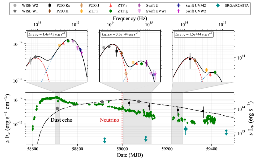
AT2019fdr, a long-duration flare (see Fig. 1) of apparent nuclear origin, was first discovered by ZTF one year prior to the neutrino detection Frederick et al. (2021); Nordin et al. (2019). AT2019fdr reached a peak flux of $1.3\times 10^{-12}~{}{\rm erg}~{}{\rm s}^{-1}~{}{\rm cm}^{-2}$ in the optical ZTF g-band on 2019, August 10, before slowly fading. With a peak g-band luminosity of $L_{\rm peak}=2.9\times 10^{44}$ erg s^-1, AT2019fdr was an extraordinarily luminous event. At the time of neutrino detection, it had decayed to $\sim 30$% of its peak flux, and was still detected by ZTF as of August 2021. Forced photometry using data from ZTF (up to 400 days prior to the flare) as well as from the Palomar Transient Facility (2010–2016) Law et al. (2009) shows no historical variability.

AT2019fdr was classified as a probable TDE, though an extreme AGN flare origin could not be ruled out (Frederick et al., 2021). High-resolution spectra yielded a redshift of $z=0.267$. Using a spectrum from the Alhambra Faint Object Spectrograph and Camera (ALFOSC), on the Nordic Optical Telescope (NOT; PI: Sollerman), a virial black hole mass estimate of $M_{\rm BH}=10^{7.55\pm 0.13}M_{\odot}$ was inferred; for further details refer to the Supplemental Material (SM).

Though the classification of AT2019fdr based on early observations included the possibility of it being a Type II superluminous supernova (SLSN-II, see Gal-Yam (2019)) Chornock et al. (2019), leading to further studies Pitik et al. (2022), its subsequent spectroscopic and photometric evolution was not consistent with expectations for SLSNe. Frederick et al. (2021) already disfavored the SLSN hypothesis based on the long-lived U-band and the UV emission, the flare’s longevity, emission at the blue end of the Balmer line profiles as well as its proximity to the nucleus of the galaxy. Here we add a late-time X-ray detection and the detection of a strong infrared echo, rendering a SLSN interpretation less likely (see below).

After discovery, AT2019fdr was also observed by the Ultraviolet and Optical Telescope (UVOT) (Roming et al., 2005) aboard the Neil Gehrels Swift Observatory (Swift) (Gehrels et al., 2004; Frederick et al., 2021). Additional observations continued up to 2020, June 7, including one epoch shortly after the neutrino detection. By that point, the transient had faded by 84% in the UVW1-band from its peak luminosity of $2.1\times 10^{44}$ erg s^-1. AT2019fdr was not detected in any of the simultaneous X-ray observations by the Swift X-ray Telescope (XRT) (Burrows et al., 2005), yielding a combined $3\sigma$ flux upper limit of $1.4\times 10^{-13}$ erg s^-1 cm^-2 for all observations before neutrino arrival (corrected for absorption).

The position of AT2019fdr was also visited by the eROSITA telescope Predehl, P. et al. (2021) aboard the Spectrum-Roentgen-Gamma (SRG) mission Sunyaev et al. (2021) four times. The first two visits did not detect an excess, with a mean flux upper limit of $2.7\times 10^{-14}$ erg s^-1 cm^-2 at the 95% confidence level. However, at the third visit on 2021, March 10–11, it detected late time X-ray emission from the transient with an energy flux of $6.2_{-2.1}^{+2.7}\times 10^{-14}$ erg s^-1 cm^-2 in the 0.3–2.0 keV band, thus showing temporal evolution in the X-ray flux (see Fig. 1). The detection displayed a very soft thermal spectrum with a best fit blackbody temperature of $56_{-26}^{+32}$ eV.

The softness of the spectrum provides further evidence for AT2019fdr being a TDE rather than regular AGN variability, where soft spectra are rare Saxton et al. (2020). Though NLSy1 galaxies generally exhibit softer X-ray spectra, the temperature of AT2019fdr is atypically low even in this context (lower than all NLSy1s in Leighly (1999) and Vaughan et al. (1999)). Furthermore, X-ray emission is rarely seen for SLSNe Margutti et al. (2018), with only the first SLSN ever observed, SCP 06F6 Barbary et al. (2008), possibly showing an X-ray flux exceeding the luminosity of AT2019fdr Gänsicke et al. (2009). This provides more evidence against the SLSN classification.

AT2019fdr was further detected at mid-infrared (MIR) wavelengths as part of routine NEOWISE survey observations Mainzer et al. (2011) by the Wide-field Infrared Survey Explorer (WISE) Wright et al. (2010). Using pre-flare archival NEOWISE data as baseline, a substantial flux increase was detected in both W1- and W2-band. MIR emission reached a peak luminosity of $1.9\times 10^{44}\rm\,erg\,s^{-1}$ on 2020, August 13, over one year after the optical/UV peak. Complementary near-infrared (NIR) measurements were taken with the P200 Wide Field Infrared Camera (WIRC, (Wilson et al., 2003)) in the J-, H- and Ks band. After subtracting a synthetic host model (see SM), a fading transient infrared signal was detected in all three bands; see Fig. 1.

We modeled this lightcurve as a composite of two unmodified blackbodies (a ‘blue’ and a ‘red’ blackbody). We interpret the time-delayed infrared emission as a dust echo: The blue blackbody heats surrounding dust, which then starts to glow. The lightcurve of this dust echo was inferred using the method described in van Velzen et al. (2016) and the corresponding fit is shown in Fig. 1. An optical/UV bolometric luminosity of $L=1.4^{+0.1}_{-0.1}\times 10^{45}$ erg s^-1 at peak was derived. By integrating this component over time, we derived a total bolometric energy of $E_{\rm bol}=3.4\times 10^{52}\rm\,erg$ (the red blackbody was not added, as dust absorption is already accounted for through the extinction correction). This is almost twice the inferred bolometric energy of ASASSN-15lh, which was one of the brightest transients ever reported Dong et al. (2016) and was suggested to be a TDE Leloudas et al. (2016). Furthermore, the energy budget, bolometric evolution and luminous dust echo suggest that AT2019fdr belongs to a class of TDE candidates observed in AGN (similar to PS1-10adi Kankare et al. (2017), AT2017gbl Kool et al. (2020) or Arp 299-B AT1 Mattila et al. (2018)). For details on the modeling methods, see SM.

Following the neutrino detection, we performed radio observations of AT2019fdr with a dedicated Very Large Array (VLA) (Perley et al., 2011) Director’s Discretionary Time (DDT) program (PI: Stein) three times over a period of four months, and obtained multi-frequency detections. AT2019fdr shows a featureless power law spectrum consistent with optically thin synchrotron emission above $\sim$ 1 GHz with no significant intrinsic evolution between the epochs (see SM). The peak flux density was $0.39\pm 0.03$ mJy in the 1–2 GHz band. The lack of apparent evolution suggests that the radio emission is not related to the transient, but rather originated from the AGN host. An additional sub-dominant transient component could be present.

No gamma rays were detected by the Fermi Large Area Telescope (Fermi-LAT) (Atwood et al., 2009) between the first detection of AT2019fdr and one year after neutrino detection, yielding an upper limit of $1.3\times 10^{-12}\,\rm erg\,s^{-1}\,cm^{-2}$ (see van Velzen et al. ).

AT2019fdr is the second probable neutrino–TDE association found by ZTF. To calculate the probability of finding two such coincident events by chance, while accounting for the fact that some TDEs will not be spectroscopically classified, we developed a broader sample of photometrically-selected ‘candidate TDEs’. We selected ‘nuclear’ transients that are at least as bright as AT2019fdr from the sample of ZTF transients, and applied cuts to identify TDE-like rise- and decay-times (see SM and van Velzen et al. for details). Our sample begins in 2018 (the ZTF survey start), and we further required a flare peak date before July 2020. We excluded only transients for which a TDE origin was ruled out through spectroscopic classification (i.e. our sample contains all unclassified candidates and all classified TDEs). To compute the sky source density at any given time, we conservatively estimated their average lifetime at 1 year after discovery, yielding an effective source density of $1.7\times 10^{-4}$ per deg² of sky in the ZTF footprint (most TDEs evolve on shorter timescales, which – if accounted for – would reduce the effective source density). When including all 24 neutrinos followed up by our program by September 2021 (covering a combined area of 154.33 deg², see SM), the probability of finding any photometrically-selected TDE candidate by chance is $2.6$ $\times 10^{-2}$, while the probability of finding two by chance is $3.4\times 10^{-4}$ (3.4$\sigma$). We emphasize that these estimates rely solely on the optical flux and a nuclear location in the host galaxy, and thus do not account for the additional luminous dust echoes or post-flare X-ray detections observed for AT2019dsg and AT2019fdr.

Neutrino emission from AT2019fdr: With a single neutrino observed in association with AT2019fdr, the inference of the neutrino flux will be subject to a large Eddington bias Strotjohann et al. (2019) and hence very uncertain. However, we can make a more robust statement on the neutrino flux by considering the underlying population (see e.g. Stein et al. (2021a)). The detection of two high-energy neutrinos implies a mean expectation for the full TDE catalog in the range $0.36<N_{\nu,\textup{tot}}<6.30$ at 90% confidence, where $N_{\nu,\textup{tot}}$ is the cumulative neutrino expectation for the nuclear transients that ZTF has observed. AT2019fdr emits $\sim 2\%$ of the g-band peak energy flux for the population of nuclear transients, consisting of the 17 published ZTF TDEs (see van Velzen et al. (2021)) and all TDE candidates as bright as AT2019fdr (see SM for the latter). If we take this as a proxy for AT2019fdr’s contribution to the neutrino emission, we would expect a total number of neutrinos $0.007\lesssim N_{\nu}\lesssim 0.13$ for this source.

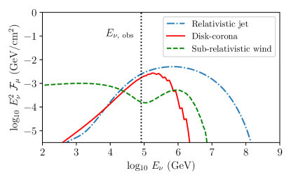
This estimate can be compared to model expectations. We present three different models invoking $p\gamma$ and/or $pp$ interactions, where protons are efficiently accelerated in a disk corona, a sub-relativistic wind or a relativistic jet (see SM). The resulting spectra are shown in Fig. 2. All models can explain the observed energy of the IC200530A neutrino event; they also make predictions for the underlying ‘neutrino lightcurve’, though this can only be resolved once many neutrinos from TDEs have been detected. The obtained neutrino luminosities $L_{\nu}\lesssim 0.1\,L_{\mathrm{Edd}}\simeq 5\times 10^{44}\rm\,erg\,s^{-1}$ are consistent with theoretical expectations for most models Winter and Lunardini (2021).

In accretion flow models Murase et al. (2020); Hayasaki and Yamazaki (2019), the virial theorem implies a cosmic ray acceleration efficiency $\eta_{\rm CR}<(1/40){(R/10\,R_{\rm S})}^{-1}$ Murase et al. (2020) for a cosmic-ray luminosity $L_{\rm CR}=\eta_{\rm CR}\dot{M}c^{2}$, where $R$ is the emission radius and $R_{\rm S}=2\,GM/c^{2}$ is the Schwarzschild radius. Even for a mass accretion rate of $\dot{M}\sim 10\,L_{\rm Edd}/c^{2}$, the neutrino luminosity would not exceed $\sim 10^{44}\rm\,erg\,s^{-1}$. In the case of AT2019fdr, the Eddington ratio $\lambda_{\rm Edd}\equiv L/L_{\rm Edd}\lesssim 0.07-0.3$ in the first 2 epochs, implying accretion near the Eddington limit around the peak and sub-Eddington accretion around the time of the neutrino detection. For such high accretion the disk plasma is collisional, while the coronal region may allow particle acceleration and non-thermal neutrino production Murase et al. (2020). This model yields $N_{\nu}\sim 0.007$ when evaluating its spectrum under the effective area of the neutrino alert channel Blaufuss et al. (2019). This is within the expected range, albeit at its lower end. The time delay is consistent with quasi-steady coronal emission. Alternatively, because the accretion rate gradually decreases, the neutrino time delay can be attributed to the formation of a collisionless corona that allows ion acceleration Murase et al. (2020).

We also considered a sub-relativistic wind with a velocity of $\sim 0.1c$, consistent with what was observed for AT2019dsg. Such a wind is naturally launched from the TDE disk (e.g., Jiang et al. (2019)), and may interact with tidal disruption debris. A strong shock is also expected from interactions between tidal streams. Ions can be accelerated at the shock via diffusive shock acceleration and produce neutrinos through inelastic $pp$ and $p\gamma$ collisions Murase et al. (2020). In this sub-relativistic wind model, the maximum proton energy can be as high as $\sim 10-100$ PeV. If the cosmic ray luminosity is three times the optical luminosity, the expected number of muon neutrinos is $N_{\nu}\sim 0.002$, which falls outside the empirical range for this baryon loading factor. The neutrino light curve would trace the wind luminosity in the calorimetric limit, and the time delay is consistent with quasi-steady radio emission.

In the relativistic jet model, external target photons from the disk are back-scattered into the jet frame. Here we followed Winter and Lunardini (2021) for AT2019dsg, but adopted a unified model Mummery (2021) to extrapolate to higher SMBH masses as given for AT2019fdr. We estimated a thermal far UV to X-ray spectrum with $T\simeq 34\,\mathrm{eV}$. This turned out to be consistent with the late-time X-ray detection within the uncertainties. The isotropization timescale of the photons is expected to be given by the system size, suggesting a possible correlation with the dust echo; as a consequence the isotropized X-ray and dust echo lightcurves look very similar. The jet model allows for efficient particle acceleration and results in a relatively large number of 0.027 neutrino events with a maximum $L_{\nu}\simeq 0.05\,L_{\mathrm{Edd}}$ thanks to the beaming effect; however, direct signatures of the jet have not been observed.

Figure 2: Neutrino fluence for the three models described here. The reported energy of the neutrino event Stein (2020a), represented by the dotted vertical line, should be viewed as a lower limit to the neutrino energy.

Conclusions: AT2019fdr was an exceptionally bright nuclear transient that was already identified in the literature as a probable TDE in an active galaxy Frederick et al. (2021). In this work, we have presented new observational data, including the identification of a strong dust echo and soft late-time X-ray emission, which further support a TDE origin for this flare.

AT2019fdr was a very long-lived transient, one of the most luminous ever detected. For a TDE, the energy release would require a very massive star Ryu et al. (2020). However, unlike for TDEs in quiescent galaxies, the AGN disk in AT2019fdr might provide the system with additional energy Chan et al. (2019). Furthermore, the post star-burst nature of the host increases the expected rate for TDEs Arcavi et al. (2014); French et al. (2020); Stone et al. (2018).

AT2019fdr was the second candidate neutrino-TDE identified by our ZTF follow-up program. While AT2019fdr was far more luminous than AT2019dsg, the first TDE associated with a high-energy neutrino, it was also more distant. As a result, the two objects have comparable bolometric energy fluxes. The probability for finding two such bright neutrino-coincident TDEs by chance is just $3.4\times 10^{-4}$, a sevenfold decrease relative to the previously-reported single association Stein et al. (2021a). The gain due to the second association is somewhat offset by the larger neutrino sample and the more inclusive candidate TDE selection. Within the framework of this paper, the association of a second object results in a reduction of the chance probability by a factor of 75 versus a single association.

AT2019fdr and AT2019dsg share other similarities beyond their potential association with a high-energy neutrino. Intriguingly, AT2019dsg also displayed an unusually strong dust echo signal van Velzen et al. , indicating that the presence of large amounts of matter and an associated high star formation rate in the environment could be a common signature for high-energy neutrino production in such systems. A dedicated search for further associations based on this signature is presented in van Velzen et al. and provides more supporting evidence for neutrino production in TDEs.

We studied neutrino emission from AT2019fdr using models previously applied to explain the observations of AT2019dsg. Similar to AT2019dsg, various plausible cosmic ray acceleration sites have been identified, such as the corona, a sub-relativistic wind, or a relativistic jet. The number of expected muon neutrinos predicted by the corona and jet models is consistent with empirical constraints derived from the two TDE-neutrino associations. All models require efficient neutrino production at a neutrino luminosity comparable to a fraction of the Eddington luminosity. The neutrino delay may be related to the size of the newly formed system (jet model) or the formation of a collisionless corona (corona model).

With two objects being associated with IceCube neutrino alerts, out of a number of 11.5 expected astrophysical neutrinos (summed alert signalness, see SM), we obtain a fraction of $18^{+38}_{-15}\%$ (90% confidence level) of astrophysical neutrinos that could be explained due to ZTF-detected TDE candidates. Accounting for the incompleteness of our sample with the procedure in (Stein et al., 2021a), our results imply that at least 7.8% of astrophysical neutrinos would come from the broader TDE population.

The search for neutrinos resulting in public alerts has a high energy threshold to reduce the background. Even when considering the full energy range of IceCube IceCube Collaboration (2018), the expected number of neutrino events from AT2019fdr remains below one. Therefore, the detection of additional lower-energy neutrinos from AT2019fdr is not expected (see also the search by the ANTARES neutrino observatory Albert et al. (2021)).

Fully understanding the role of TDEs as particle accelerators will only be possible with comprehensive multi-wavelength and -messenger data. While the detailed production processes remain uncertain, the observations presented here provide further evidence that TDEs are highly efficient sources of high-energy neutrinos.

I Correspondence

Correspondence and requests for materials should be addressed to Marek Kowalski (marek.kowalski@desy.de) and Simeon Reusch (simeon.reusch@desy.de).

II Acknowledgments

S.R. acknowledges support by the Helmholtz Weizmann Research School on Multimessenger Astronomy, funded through the Initiative and Networking Fund of the Helmholtz Association, DESY, the Weizmann Institute, the Humboldt University of Berlin, and the University of Potsdam. A.F. acknowledges support by the Initiative and Networking Fund of the Helmholtz Association through the Young Investigator Group program (A.F.). C.L. acknowledges support from the National Science Foundation (NSF) with grant number PHY-2012195. The work of K.M. is supported by the NSF Grant No. AST-1908689, No. AST-2108466 and No. AST-2108467, and KAKENHI No. 20H01901 and No. 20H05852. M.C. acknowledges support from the National Science Foundation with grant numbers PHY-2010970 and OAC-2117997. S.S. acknowledges support from the G.R.E.A.T research environment, funded by Vetenskapsrådet, the Swedish Research Council, project number 2016-06012. M.G., P.M. and R.S. acknowledge the partial support of this research by grant 19-12-00369 from the Russian Science Foundation. S.B. acknowledges financial support by the European Research Council for the ERC Starting grant MessMapp, under contract no. 949555. A.G.Y.’s research is supported by the EU via ERC grant No. 725161, the ISF GW excellence center, an IMOS space infrastructure grant and BSF/Transformative and GIF grants, as well as The Benoziyo Endowment Fund for the Advancement of Science, the Deloro Institute for Advanced Research in Space and Optics, The Veronika A. Rabl Physics Discretionary Fund, Minerva, Yeda-Sela and the Schwartz/Reisman Collaborative Science Program; A.G.Y. is the incumbent of the The Arlyn Imberman Professorial Chair. E.C.K. acknowledges support from the G.R.E.A.T research environment funded by Vetenskapsrådet, the Swedish Research Council, under project number 2016-06012, and support from The Wenner-Gren Foundations. M.R. has received funding from the European Research Council (ERC) under the European Union’s Horizon 2020 Research and Innovation Program (Grant Agreement No. 759194 - USNAC). N.L.S. is funded by the Deutsche Forschungsgemeinschaft (DFG, German Research Foundation) via the Walter Benjamin program – 461903330.

Based on observations obtained with the Samuel Oschin Telescope 48-inch and the 60-inch Telescope at the Palomar Observatory as part of the Zwicky Transient Facility project. ZTF is supported by the National Science Foundation under Grant No. AST-1440341 (until 2020 December 1) and No. AST-2034437 and a collaboration including Caltech, IPAC, the Weizmann Institute for Science, the Oskar Klein Center at Stockholm University, the University of Maryland, Deutsches Elektronen-Synchrotron and Humboldt University, the TANGO Consortium of Taiwan, the University of Wisconsin at Milwaukee, Trinity College Dublin, Lawrence Livermore National Laboratories, IN2P3, University of Warwick, Ruhr University Bochum and Northwestern University. Operations are conducted by COO, IPAC, and UW.

This work was supported by the GROWTH (Global Relay of Observatories Watching Transients Happen) project funded by the National Science Foundation Partnership in International Research and Education program under Grant No 1545949. GROWTH is a collaborative project between California Institute of Technology (USA), Pomona College (USA), San Diego State University (USA), Los Alamos National Laboratory (USA), University of Maryland College Park (USA), University of Wisconsin Milwaukee (USA), Tokyo Institute of Technology (Japan), National Central University (Taiwan), Indian Institute of Astrophysics (India), Inter-University Center for Astronomy and Astrophysics (India), Weizmann Institute of Science (Israel), The Oskar Klein Centre at Stockholm University (Sweden), Humboldt University (Germany).

This work is based on observations with the eROSITA telescope on board the SRG observatory. The SRG observatory was built by Roskosmos in the interests of the Russian Academy of Sciences represented by its Space Research Institute (IKI) in the framework of the Russian Federal Space Program, with the participation of the Deutsches Zentrum für Luft- und Raumfahrt (DLR). The SRG/eROSITA X-ray telescope was built by a consortium of German Institutes led by MPE, and supported by DLR. The SRG spacecraft was designed, built, launched, and is operated by the Lavochkin Association and its subcontractors. The science data are downlinked via the Deep Space Network Antennae in Bear Lakes, Ussurijsk, and Baykonur, funded by Roskosmos. The eROSITA data used in this work were processed using the eSASS software system developed by the German eROSITA consortium and proprietary data reduction and analysis software developed by the Russian eROSITA Consortium.

This work was supported by the Australian government through the Australian Research Council’s Discovery Projects funding scheme (DP200102471).

This work includes data products from the Near-Earth Object Wide-field Infrared Survey Explorer (NEOWISE), which is a project of the Jet Propulsion Laboratory/California Institute of Technology. NEOWISE is funded by the National Aeronautics and Space Administration.

The National Radio Astronomy Observatory is a facility of the National Science Foundation operated under cooperative agreement by Associated Universities, Inc.

Based on observations made with the Nordic Optical Telescope, owned in collaboration by the University of Turku and Aarhus University, and operated jointly by Aarhus University, the University of Turku and the University of Oslo, representing Denmark, Finland and Norway, the University of Iceland and Stockholm University at the Observatorio del Roque de los Muchachos, La Palma, Spain, of the Instituto de Astrofisica de Canarias.

III Author Contributions

S.R. first identified AT2019fdr as a candidate neutrino source, performed the SED and the dust echo analysis and was the primary author of the manuscript. A.F., M.K., R.St. and S.v.V. contributed to the manuscript, the data analysis and the source modeling. A.F. and M.K. have initiated the ZTF neutrino follow-up program. C.L., K.M. and W.W. performed the neutrino production analysis. J.C.A.M.-J. contributed the VLA observations. M.Gi. performed the SRG/eROSITA observations and data analysis. S.B. and S.Ga. analyzed the Fermi data. S.R. analyzed the Swift-XRT data. S.A., K.D. and S.R. performed and analyzed the P200 IR observations. S.Ge. and S.S. requested and reduced the Swift-UVOT data. V.S.P. contributed the black hole mass estimate. E.Z. contributed to the neutrino event rate calculation. M.G. analyzed the archival radio data. S.S.K and B.T.Z. performed parts of the neutrino production analysis. V.K. and N.L.S. contributed PTF forced photometry. C.B., T.S. and J.S. ruled out other candidates in the follow-up. T.A., M.W.C., M.M.K. and L.P.S. enabled ZTF ToO observations. J.Ne., S.R. and R.St. developed the analysis pipeline. V.B., J.No. and J.v.S. developed AMPEL, and contributed to the ToO analysis infrastructure. E.C.B., S.B.C., R.D., M.J.G., R.R.L., B.R., M.R. and R.W. contributed to the implementation of ZTF. P.M. and R.Su. contributed to the implementation of SRG/eROSITA. S.F., S.Ge., A.G.-Y., A.K.H.K, E.K. and D.A.P. contributed comments/to discussions. All authors reviewed the contents of the manuscript.

IV Supplemental Material

The data and code used for the analysis presented in this paper can be accessed at https://github.com/simeonreusch/at2019fdr Reusch (2022). nuztf, the multimessenger-pipeline used to identify AT2019fdr as potential source, can be found here: https://github.com/desy-multimessenger/nuztf. Both make use of AMPEL Nordin, J. et al. (2019) and ztfquery Rigault (2018).

Follow-up of IC200530A

The high-energy neutrino IC200530A was the tenth alert followed up with our ZTF neutrino follow-up program. It had an estimated $59\%$ probability of being of astrophysical origin, based solely on the reconstructed energy of 82.2 TeV and its zenith angle (Stein, 2020a), with a best-fit position of $\text{RA[J2000]}=255.37^{+2.48}_{-2.57}$ and $\text{Dec[J2000]}=+26.61^{+2.33}_{-2.57}$ at 90% confidence level. The reported localization amounts to a projected rectangular uncertainty area of $25.38\,\rm deg^{2}$. During ZTF follow-up observations, 87% of that area was observed (accounting for chip gaps).

For a full overview of all the neutrino alerts followed up as part of our program, see Table 6. ANTARES did not report any neutrinos from the same direction Albert et al. (2021), though the corresponding upper limits reported are not constraining for the neutrino production models introduced in this work.

AT2019fdr, at a location of RA[J2000] $=257.2786$ and Dec[J2000] $=+26.8557$, was lying within the 90% localization region of IC200530A. It was consistent with arising from the nucleus of its host galaxy (SDSSCGB 6856.2), with a mean angular separation to the host position as reported in Gaia Data Release 2 (Gaia Collaboration, 2018) of $0.03\pm 0.15$ arcsec. The angular separation from the neutrino best fit position was $1.72$ deg. The event had a spectroscopic redshift of $z=0.267$, which implies a luminosity distance $D_{\rm L}\approx$ 1360 Mpc, assuming a flat cosmology with $\Omega_{\Lambda}=0.7$ and $H_{0}=70$ km s^-1 Mpc^-1.

Gamma ray limits

Details on the Fermi-LAT analysis and the upper limits can be found in van Velzen et al. . The High Altitude Water Cherenkov Experiment (HAWC) reported that no significant detection was found at the time of neutrino arrival Ayala (2020). A non-detection was also reported by the International Gamma-Ray Astrophysics Laboratory (INTEGRAL) Savchenko (2020).

X-ray observations

In the course of its ongoing all sky survey, the SRG observatory Sunyaev et al. (2021) visited AT2019fdr four times with its 6 month cadence, the first visit having taken place on 2020, March 13–14. The source was detected by eROSITA Predehl, P. et al. (2021) only once, during the third visit on 2021, March 10–11, providing evidence for temporal evolution in the X-ray emission of the source. Constraints on the flux from all three epochs are shown in Fig. 3 and listed in Table 1.

The single detection of AT2019fdr revealed a very soft thermal spectrum with a best-fit blackbody temperature of $56_{-26}^{+32}\rm\,eV$ (errors are 68% for one parameter of interest). In the rest frame of the source this corresponds to a temperature of $71_{-33}^{+41}\rm\,eV$ and is among the softest X-ray spectra of all TDEs so far detected by SRG/eROSITA Sazonov et al. (2021). The best fit value of the equivalent hydrogen column density ${\rm NH}=1.47_{-1.25}^{+2.80}\times 10^{21}\rm\,cm^{-2}$ is consistent, within the errors, with the Galactic value of ${\rm NH_{\rm Gal}}=0.40\times 10^{21}\rm\,cm^{-2}$ Ben Bekhti et al. (2016). As is usually the case for soft sources, there is some degree of degeneracy between the neutral hydrogen column density and the temperature. However, the upper bound on the temperature is still fairly low, $T_{\rm bb}<131$ eV at the 95% confidence level.

Prior to the detection of IC200530A, Swift-XRT had already observed AT2019fdr on 14 occasions (Frederick et al., 2021). Following the identification of AT2019fdr as a candidate neutrino source, an additional prompt ToO observation of the object was requested, which was conducted on 2020, June 7 (2000 second exposure).

To reduce the data and generate a lightcurve, the publicly available Swift XRT data products generator Centre (2020) was used for the energy range 0.3–10 keV. Further details can be found at (Evans et al., 2009). Since the event was not detected in any individual XRT pointings, the 14 observations prior to neutrino arrival were binned (20700 seconds in total) to compute a 3$\sigma$ energy flux upper limit of $1.4\times 10^{-13}\rm\,erg\,s^{-1}\,cm^{-2}$. The observation after neutrino arrival yielded a 3$\sigma$ energy flux upper limit of $4.7\times 10^{-12}\rm\,erg\,s^{-1}\,cm^{-2}$. To convert photon counts to energy flux, the HEASARC WebPIMMS tool Arida and Sabol (2020) was employed, using the SRG/eROSITA blackbody temperature of 56 eV. Absorption was corrected with the best-fit equivalent hydrogen column density from the same measurement (see above).

MJD	Date	Upper limit (95% CL)	Energy flux
		[$\rm erg\,s^{-1}\,cm^{-2}$]	[$\rm erg\,s^{-1}\,cm^{-2}$]
58922	2020-03-14	$2.5\times 10^{-14}$	–
59105	2020-09-13	$2.9\times 10^{-14}$	–
59284	2021-03-11	–	$6.2_{-2.1}^{+2.7}\times 10^{-14}$
59465	2021-09-08	$5.3\times 10^{-14}$	–

Table 1: SRG/eROSITA detection and upper limits in the 0.3–2.0 keV band.

Optical/UV observations

The ZTF observations were analyzed using dedicated forced photometry, yielding higher precision than ‘alert’ photometry by incorporating knowledge of the transient’s position derived from all available images. This was done using the ztffps pipeline (Reusch, 2021), which is built upon ztflc (Rigault, 2020).

To obtain Swift measurements, we retrieved the science-ready data from the Swift archive (https://www.swift.ac.uk/swift_portal). We co-added all sky exposures for a given epoch and filter to boost the signal-to-noise ratio using uvotimsum in HEAsoft (https://heasarc.gsfc.nasa.gov/docs/software/heasoft/, v6.26.1). Afterwards, we measured the brightness of the transient with the Swift tool uvotsource. The source aperture had a radius of 3 arcsec, while the background region had a significantly larger radius. The photometry was calibrated with the latest calibration files from September 2020 and converted to the AB system using the methods of Breeveld et al. (2011). All measurements were host subtracted using the synthetic host model described in the next section.

Infrared observations

Four epochs of observations were taken in the J-, H- and Ks-band with the WIRC camera (Wilson et al., 2003) mounted on the Palomar P200 telescope in 2020 on July 1 and September 27, as well as in 2021 on February 2 and May 28. The WIRC measurements were reduced using a custom pipeline described in De et al. (2020). This pipeline performs flat fielding, background subtraction and astrometry (with respect to Gaia DR2) on the dithered images followed by stacking of the individual frames for each filter and epoch. Photometric calibration was performed on the stacked images using stars from the Two Micron All Sky Survey (2MASS) Skrutskie et al. (2006) in the WIRC field to derive a zero point for the stacked images.

The combined host and flare flux was extracted from the stacked images using GALFIT Peng et al. (2002) to avoid contamination from blending with a close neighboring galaxy. photutils Bradley et al. (2020) was used to derive the Point Spread Function (PSF) for each image. For this purpose, 3–5 isolated stars which were neither dim nor bright were selected by visual inspection of the surrounding area. Based on these, the PSF in the images was fitted. The subtraction quality was verified through visual inspection of the residuals of 4 nearby reference stars from the Sloan Digital Sky Survey (SDSS) York et al. (2000). Following this, Sérsic profiles were fitted to AT2019fdr’s host galaxy and to the neighboring galaxy. Additionally, a point source was fitted.

All parameters except the point source flux were fixed after fitting one epoch (reference epoch). The point source flux was then fit in the other epochs. As the choice of reference epoch had an impact on the flux estimate, both the first and the last epoch were used as such. The difference in the point source flux estimate between both was taken to serve as the systematic uncertainty.

The host galaxy flux was estimated by fitting a galaxy model following the method of van Velzen et al. (2020). The UV flux was measured with images from the Galaxy Evolution Explorer (GALEX) Martin et al. (2005), using the gPhoton software Million et al. (2016) with an aperture of 4 arcsec. The optical flux of the host was obtained from the SDSS model magnitudes Stoughton et al. (2002). The baseline WISE data points mentioned above were also included, as was an archival measurement from the UKIRT Infrared Deep Sky Survey (UKIDSS) Lawrence et al. (2007). The prospector software was employed to sample synthetic galaxy models built by Flexible Stellar Population Synthesis (FSPS, Conroy and Gunn (2010); Foreman-Mackey et al. (2014)). An overview of the values used for constructing the model can be seen in Table 3.

MJD	Date	J-band	H-band	Ks-band
59031	2020-07-01	$19.06\pm 0.50$	$17.73\pm 0.12$	$17.13\pm 0.26$
59121	2020-09-29	$19.78\pm 0.98$	$17.76\pm 0.12$	$17.45\pm 0.35$
59249	2021-02-04	–	$18.26\pm 0.19$	$17.81\pm 0.48$
59362	2021-05-28	–	$18.42\pm 0.22$	$17.91\pm 0.53$
		W1-band	W2-band
58709	2019-08-14	$17.18\pm 0.11$	$17.08\pm 0.23$
58910	2020-03-02	$16.49\pm 0.07$	$16.37\pm 0.11$
59074	2020-08-13	$16.47\pm 0.09$	$16.20\pm 0.11$

Table 2: Top: NIR AB magnitudes after subtraction of the synthetic host model. Only systematic uncertainties are given (photometric uncertainties should be negligible in comparison, at least in the J- and H-band). The third and fourth J-band epochs had negative flux after host-model subtraction, which are counted as non-detections. Bottom: MIR AB magnitudes after subtracting the pre-peak baseline.

Band	AB magnitude
GALEX FUV	$22.32^{+0.07}_{-0.10}$
GALEX NUV	$21.52^{+0.06}_{-0.10}$
SDSS u	$20.91^{+0.06}_{-0.07}$
SDSS g	$19.97^{+0.04}_{-0.04}$
SDSS r	$19.00^{+0.02}_{-0.03}$
SDSS i	$18.64^{+0.02}_{-0.03}$
SDSS z	$18.36^{+0.02}_{-0.03}$
UKIRT J	$18.18$
WISE W1	$17.83^{+0.05}_{-0.05}$
WISE W2	$17.78^{+0.03}_{-0.05}$

Table 3: Archival measurements from GALEX, SDSS, UKIRT (the isoMag value was given without error) and WISE. These were used to build the synthetic host model.

In addition to the ground-based NIR observations, photometry was extracted from MIR images of the WISE Wright et al. (2010) satellite. For this the W1- and the W2-band were used, centered at 3.4 and 4.6 $\mu$m, respectively. The WISE and NEOWISE (the new designation after a hibernation period, Mainzer et al. (2011)) photometry at the location of AT2019fdr suffered from blending with a nearby galaxy, so forced PSF photometry was used (Jones et al., 2015) on the co-added images Masci (2013). These images were binned in 6 month intervals, aligned to the observing pattern of the satellite. The WISE flux in the 13 epochs prior to the optical flare was used to define a baseline, from which difference flux was then computed. We measured a significant flux increase from this baseline. In the W1-band, the root mean square (RMS) variability of the baseline was only 18 $\mu$Jy , which is much smaller than the peak difference flux of 0.9 mJy.

The infrared brightness over time, as detected by P200 and WISE after subtracting the host baseline contribution, is shown in Table 2.

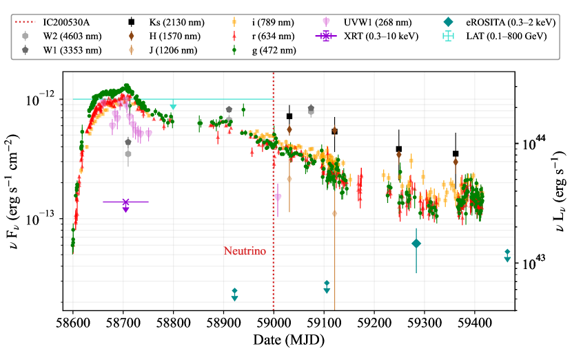
A selection of IR, optical and UV data are shown in Figure 3, alongside upper limits from Swift-XRT and Fermi-LAT, as well as the measurements from SRG/eROSITA.

Figure 3: Lightcurve of AT2019fdr, showing host-subtracted ZTF, WISE, P200 and Swift-UVOT photometry, non host-subtracted SRG/eROSITA photometry, as well as binned Swift-XRT and Fermi-LAT upper limits (the former has been corrected for absorption). The dotted vertical line indicates the arrival time of the IceCube neutrino IC200530A.

Radio observations

We observed AT2019fdr with a dedicated Karl G. Jansky Very Large Array (VLA) Director’s Discretionary Time (DDT) program VLA/20A-566 (PI: Stein), and obtained multi-frequency detections at three epochs. The individual observations were taken in 2020 on July 3, September 13 and November 7. The array was in its moderately-extended B configuration for the first two observations, and in the hybrid BnA configuration (with a more extended northern arm) for the final epoch. The first observation was performed in the 2–4 and 8–12 GHz bands, to which we added the 1–2 and 4–8 GHz bands in the subsequent epochs. We used 3C 286 for the delay, bandpass, and flux calibration, and the nearby source J1716+2152 for the complex gain calibration. We followed standard procedures for the external gain calibration, which were performed with the VLA calibration pipeline, using the Common Astronomy Software Application (CASA) v5.6.2. The source was then imaged in each observed band with the CASA task tclean, using Briggs weighting with a robust factor of 1 as a compromise between sensitivity and resolution. The target flux density was measured by fitting a point source in the image plane.

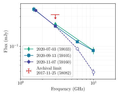
While consistent flux densities were measured in the 2–4 and 8–12 GHz bands in the first two observations, the final epoch suggested a possible spectral steepening, with reduced flux densities in the 4–8 and 8–12 GHz bands (see Fig. 4). However, extensive testing revealed that this apparent spectral steepening was not intrinsic to the source. We interpolated the gains derived on the first, third and last of the five 8–12 GHz scans on J1716+2152 to the remaining two scans, deriving their calibration in the same way as for AT2019dsg (see Stein et al. (2021a)). The measured calibrator flux densities for those two scans were found to be significantly lower than for the other three. This implied significant atmospheric phase changes between calibrator scans, which reduced the measured flux densities due to decorrelation. Without sufficient flux density in the target field to apply self-calibration, we were unable to correct for this effect, which is worst at the highest frequencies. Therefore, no evidence for intrinsic source variability can be found in the radio band across the 5 months of observations.

Additionally, an archival upper limit was obtained from the Very Large Array Sky Survey (VLASS) Lacy et al. (2020), which was the only sky survey with adequate sensitivity and angular resolution to probe the emission on the angular and flux density scales relevant for AT2019fdr. The quicklook continuum fits image for tile T17t23We was downloaded from the archive (https://archive-new.nrao.edu/vlass/quicklook/) and dates to 2017, November 25 (2–4 GHz band). No emission was detected at a $3\sigma$ significance, where $\sigma=0.11$ mJy/beam is the local RMS noise and the beam is 2.46 arcsec $\times$ 2.28 arcsec (position angle $=-37^{\circ}$), resulting in an upper limit of $0.32\rm\,mJy$. This result is fully consistent with what was measured in the same band in our dedicated observations. A more recent observation from VLASS epoch 2 was taken very close to the second dedicated observation (2020, September 6), but the local noise was slightly larger and the $3\sigma$ upper limit was less constraining ($0.4\rm\,mJy$).

All our measurements, as well as the archival limit from VLASS are shown in Fig. 4 and Table 4.

The observed radio spectra can be described by synchrotron emission from a population of relativistic electrons. These electrons were assumed to be accelerated into a power-law distribution in energy, which leads to a power law in the unattenuated synchrotron spectrum. No break in the power-law spectrum was observed. Therefore the peak frequency, where synchrotron self-absorption sets in, is expected to lie below the lowest observed frequency. The data was analyzed using the models from Barniol Duran et al. (2013); Stein et al. (2021a). This allowed to infer energies of a few times $10^{50}$ erg for the electron population, under the assumption of equipartition; a peak flux of 0.5 mJy at 1 GHz; and neglecting the impact of baryons. This value provides a lower limit on the non-thermal energy of the system. Given that electrons are typically accelerated with much lower efficiency than protons in astrophysical accelerators Morlino and Caprioli (2012), they were assumed to carry 10% of the energy carried by relativistic protons ($\epsilon_{e}=0.1$). Furthermore, the magnetic field was assumed to carry $0.1\%$ of the total energy ($\epsilon_{B}=10^{-3}$), as indicated by radio observations of TDEs (Eftekhari et al., 2018) and supernovae (Horesh et al., 2013). Under these assumptions, the total energy energy in non-thermal particles was inferred to be $\sim 10^{52}$ erg. The inferred size of the emission region, $\sim 10^{18}$ cm, and the lack of temporal evolution suggest that the emission was primarily powered by an outflow that was active already prior to the transient event. A second, sub-dominated component could be present. Since the radio observations cover only a period of 5 months, a fast-varying transient signal would be easier to constrain than a slower one. For instance, a relativistic jet viewed face-on would show faster variations and dominate the radio flux if sufficiently energetic, while an off-axis relativistic jet could escape detection due to Doppler deboosting of its radio flux (the latter explanation only works up to the point the jet decelerates and starts to emit isotropically, see e.g. Generozov et al. (2017)).

Figure 4: Three epochs of VLA measurements of AT2019fdr, as well as the VLASS archival upper limit. Note: The apparent spectral steepening in our third epoch (empty circular markers) appears not to be intrinsic to the source, but due to systematic effects.

MJD	Date	Band	Flux density
		[GHz]	[$\mu$ Jansky]
58032	2017-11-25	3.00	$\leq 320$
59033	2020-07-03	3.00	$226\pm 13$
59033	2020-07-03	10.00	$86\pm 11$
59105	2020-09-13	1.52	$390\pm 34$
59105	2020-09-13	3.00	$211\pm 10$
59105	2020-09-13	6.00	$118\pm 6$
59105	2020-09-13	10.00	$86\pm 5$
59160	2020-11-07	1.62	$373\pm 20$
59160	2020-11-07	3.00	$209\pm 9$
59160	2020-11-07	6.00	$91\pm 6$
59160	2020-11-07	10.00	$39\pm 5$

Table 4: VLA measurements and the VLASS archival limit (first row).

Double-blackbody fit

The SED was fit using the lmfit Python package (Newville et al., 2021) with both a broken and a non-broken intrinsic power law, as well as a single and a double unmodified blackbody spectrum. The data are well described by a double-blackbody model, comprised of an optical/UV ‘blue’ blackbody and an infrared ‘red’ blackbody. Fitting is done for three epochs during which infrared, optical and UV data is available. These epochs in MJD are: 1) 58700–58720, 2) 59006–59130 and 3) 59220–59271. To account for host extinction, we employed extinction Kyle (2016) using the Calzetti attenuation law Calzetti et al. (2000). The extinction parameter $A_{V}$ was left free in epoch 1 and was fixed at the epoch 1 best-fit value ($A_{V}=0.45^{+0.14}_{-0.14}$ mag for $R_{V}=3.1$) for epochs 2 and 3. We chose epoch 1 to determine the extinction parameter because the observations of the optical/UV are most precise there.

The other fit parameters were the blackbody temperature and the the blackbody radius, resulting in a total of 6 fit parameters in epoch 1, and 4 in epochs 2 and 3. The model was fitted to the data in the three epochs using the Levenberg-Marquardt minimization algorithm. 68% confidence levels for all parameters were estimated by determining $\Delta\chi^{2}=1$ relative to the best-fit $\chi^{2}$, stepping through each parameter while leaving the other parameters free during minimization.

The best fit blackbody values are shown in Table 5; the respective SEDs for the three epochs are shown in the top panels of Fig. 1 in the main text.

Epoch	Band	Temp.	Radius	Luminosity
		[K]	[cm]	[erg s-1]
1	O+UV	$13526^{+569}_{-574}$	$7.8^{+0.4}_{-0.4}\times 10^{15}$	$1.4^{+0.1}_{-0.1}\times 10^{45}$
	IR	$1505^{+421}_{-313}$	$2.2^{+1.6}_{-1.4}\times 10^{17}$	$1.7^{+2.2}_{-1.0}\times 10^{44}$
2	O+UV	$11731^{+663}_{-683}$	$4.9^{+0.4}_{-0.4}\times 10^{15}$	$3.3^{+0.3}_{-0.4}\times 10^{44}$
	IR	$1762^{+121}_{-124}$	$2.5^{+0.2}_{-0.2}\times 10^{17}$	$4.3^{+0.5}_{-0.7}\times 10^{44}$
3	O+UV	$10230^{+2373}_{-1645}$	$4.3^{+3.3}_{-1.0}\times 10^{15}$	$1.5^{+1.2}_{-0.4}\times 10^{44}$
	IR	$2237^{+402}_{-462}$	$1.0^{+0.6}_{-0.4}\times 10^{17}$	$1.9^{+1.4}_{-0.5}\times 10^{44}$

Table 5: Blackbody fit values for three epochs (1–3), where ‘O+UV’ denotes the blue blackbody in the optical/UV and ‘IR’ denotes the red infrared blackbody. The luminosity is given dereddened and in the source frame and the uncertainties are at 68% confidence level. Note that the O+UV temperature and radius (and therefore the luminosity) in the third epoch are not well constrained, as there are no late-time UV measurements available. The same holds true for the infrared blackbody in the first and the last epoch, as only 2 data points are available in the infrared.

Dust echo model and energy output

Following the procedure in van Velzen et al. (2016), the optical lightcurve was convolved with a rectangular function of width $2\times\Delta t_{c}$, where $\Delta t_{c}$ is the light travel time from the transient to the surrounding dust region. A best-fit value of $\Delta t_{c}=193$ days was obtained, which translates to a distance to the dust region of $5\times 10^{17}\rm\,cm$ ($0.16\rm\,pc$). To obtain a measure for the peak luminosity of the transient, the blue blackbody fit at peak was used. The resulting unobscured peak luminosity from the blue blackbody was $L_{\rm peak}=1.4^{+0.1}_{-0.1}\times 10^{45}\rm\,erg\,s^{-1}$. To check this value for consistency, the peak optical/UV luminosity was also calculated following van Velzen et al. (2016). This method relies only on the blackbody temperature (normalized to $1850\rm\,K$) and the radius of the dust region, normalized to $0.1\rm\,pc$ (assuming a dust grain size of $0.1\,\mu\rm m$):

$$L_{\rm peak}=5\times 10^{44}R^{2}_{0.1}T^{5.8}_{1850}\rm\,erg\,s^{-1}$$

This yielded a value of $L_{\rm peak}=1.3\times 10^{45}\rm\,erg\,s^{-1}$, which is in good agreement with the value derived from the blackbody fit described in the section above.

As the temperature of the optical/UV blackbody decreases only slightly and stays roughly centered on the g-band, the total energy radiated in the optical/UV can be approximated by scaling the peak luminosity with the g-band lightcurve and integrating over time. The resulting energy output was $E_{\rm O+UV}=3.4\times 10^{52}\rm\,erg$.

The peak dust echo luminosity was inferred from the IR blackbody fit to be $L_{\rm dust}=4.3\times 10^{44}$ erg s^-1. Similarly to the optical/UV, we time-integrated the fitted dust echo lightcurve, normalized to the peak dust echo luminosity from epoch 2, to obtain the total bolometric energy of the dust echo: $E_{\rm dust}=1.1\times 10^{52}$ erg. The ratio of the two time-integrated energies resulted in an unusually high covering factor of $1/3$, while the TDE dust echoes in quiescent galaxies typically show covering factors of around 1% van Velzen et al. (2016).

Black hole mass

The commonly adopted method to derive the mass of the central SMBH ($M_{\rm BH}$) of an AGN is using its optical spectrum and is called the single-epoch virial technique (see e.g. Vestergaard and Peterson (2006)). The NOT spectrum used for this was taken on 2020, April 30 with the ALFOSC camera. There are later spectra, but these do not contain the H$\alpha$ emission line. The spectrum was reduced in a standard way, consisting of wavelength calibration through an arc lamp and flux calibration using a spectrophotometric standard star.

The publicly available multi-component spectral fitting tool PyQSOFit Guo et al. (2018) was used for spectral analysis. We brought the spectrum to the lab frame and dereddened it using the Milky Way extinction law of Fitzpatrick (1999) with $R_{\rm V}=3.1$ and dust map data adopted from Schlegel et al. (1998) – note that the extinction law is not the same as the one used in the blackbody fits, but the difference is small. The continuum was modeled using line-free regions as a combination of a third degree polynomial and an optical Fe II template adopted from Boroson and Green (1992). It was subtracted from the spectrum to obtain the line spectrum only. The H$\alpha$ and H$\beta$ line complexes were then fitted separately, while simultaneously fitting the emission lines in each complex. In the wavelength range of [6400,6800] Å, the H$\alpha$ emission line was modeled with three Gaussian functions, two for the broad components and one for the narrow. [N ii] $\lambda\lambda$6548,6584, and [S ii] $\lambda\lambda$6717,6731 were also fitted with a single Gaussian. The H$\beta$ emission line was fitted in the wavelength range [4700,5100] Å, similar to the H$\alpha$ line. Finally, the [O iii] $\lambda\lambda$4959,5007 doublet was modeled with two Gaussian functions. The estimated uncertainties are statistical only and do not include the intrinsic scatter (0.3$-$0.4 dex) associated with the virial approach (see e.g. Vestergaard and Peterson (2006); Shen et al. (2011)). Further details about the fitting technique and PyQSOFit can be found in Guo et al. (2019) and Shen et al. (2019). The fitted spectrum is shown in Figure 5.

Figure 5: The top plot shows the NOT spectrum of AT2019fdr analyzed with PyQSOFit; different line components are labeled. The bottom panels show zoomed versions of the fitted line complexes.

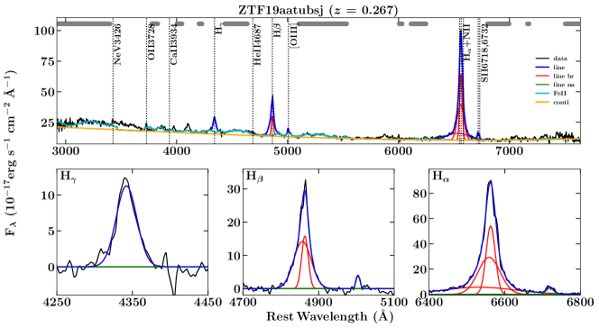
The measured full-width-at-half-maximum (FWHM) of the H$\beta$ line was $1914\pm 282$ km s^-1 and the continuum luminosity at 5100 Å was $\lambda L_{\lambda}=44.16\pm 0.01$ (log-scale, erg s^-1). Broadening due to limited detector resolution was considered to be small. From the estimated FWHM and $\lambda L_{\lambda}$, the mass of the central black hole was computed by adopting the following empirical relation Shen et al. (2011):

$$\scriptstyle\log\left(\frac{M_{\rm BH,vir}}{M_{\odot}}\right)=a+b\log\left(\frac{\lambda L_{\lambda}}{10^{44}\,{\rm erg/s}}\right)+2\log\left(\frac{\rm FWHM}{\rm km/s}\right)$$

The coefficients $a$ and $b$ were taken as 0.91 and 0.5, adopted from Vestergaard and Peterson (2006). This resulted in $M_{\rm BH}=10^{7.55\pm 0.13}M_{\odot}$. Shen et al. (2011) also give the following empirical relation to estimate $M_{\rm BH}$ from the H$\alpha$ line FWHM and luminosity:

$$\scriptstyle\log\left(\frac{M_{\rm BH,vir}}{M_{\odot}}\right)_{\rm H\alpha}=~{}0.379+0.43\log\left(\frac{L_{\rm H\alpha}}{10^{42}\rm erg/s}\right)+2.1\log\left(\frac{\rm FWHM_{H\alpha}}{\rm km/s}\right)$$

Supplying the derived H_α FWHM ($1753\pm 246\rm\,km\,s^{-1}$) and luminosity (43.05$\pm$0.06, log-scale, erg s^-1) in the above equation, $M_{\text{BH}}$ was computed as $10^{7.64\pm 0.13}M_{\odot}$, consistent with the previous estimate.

These estimates are consistent with the masses derived in the NLSy1 ZTF study Frederick et al. (2021), which employed two different methods. The virial approach (also used above) yielded an estimate of $10^{7.1}M_{\odot}$, while an approach using the host galaxy luminosity according to McLure and Dunlop (2002) resulted in $10^{7.8}M_{\odot}$. In this paper an Eddington ratio of $\frac{L}{L_{\text{Edd}}}=0.24-1.2$ was derived. The different result for the virial approach can be explained by the fact that Frederick et al. (2021) fit a single Lorentzian profile while here a multi-Gaussian approach is used. Also, the spectrum employed for the fit presented here was more recent, presumably containing less transient emission.

Chance coincidence

To compute the chance coincidence of finding an event like AT2019fdr in association with a high-energy neutrino, we obtained the full set of nuclear ZTF transient flares as selected by AMPEL Nordin, J. et al. (2019); Patterson et al. (2019) from the ZTF alert stream Masci et al. (2019). At least 10 detections in both g- and r-band were required, as was a weighted host–flare offset $\leq 0.5$ arcsec and a majority of the data points having positive flux after subtracting the reference image. The dataset was further restricted to transients being first detected after 2018 January 1 and peaking before July 2020. 3172 flares survived these cuts.

We further required the nuclear transients not to be classified as (variable) star or bogus object (e.g. subtraction artifacts); additionally, flares were rejected when their rise (fade) $e$-folding time (see van Velzen et al. (2021) for details) was smaller than the uncertainty on this value; these two cuts left 1628 candidates. As we were only interested in events of brightness comparable to AT2019fdr, we required that the peak apparent magnitude (see van Velzen et al. for details) $\leq$ the peak magnitude of AT2019fdr; this left 157 events. Furthermore, the rise (fade) $e$-folding time was required to be in the [15, 80] ([30, 500]) day interval to select for (candidate) TDEs, resulting in 25 transients.

Nuclear transients which have been spectroscopically classified as supernovae were excluded from the remaining 25 events. Furthermore, we visually excluded transients showing only short-timescale AGN variability, displaying no consistent color or color evolution and events which were not sufficiently smooth post peak. This procedure left a final sample of 12 transients.

To calculate the effective source density of these 12 events, their lifetime was conservatively estimated at 1 year per event. The ZTF survey footprint is $28000\rm\,deg^{2}$ (excluding sources with galactic latitude $|b|<7$) Stein et al. (2021a). From the time range of the sample (2.5 years) and the ZTF footprint, the effective source density was computed as $1.7\times 10^{-4}\rm\,deg^{-2}$. This is the density of sources per $\rm\,deg^{2}$ of sky in the survey footprint at any given time. Through multiplying the effective source density by the combined IceCube alert footprint of $154.3\rm\,deg^{2}$, an expectation value for the number of neutrinos can be calculated. Employing a Poisson distribution, the chance coincidence of finding 2 sources by chance was calculated as $p=3.4\times 10^{-4}$ ($p=2.6\times 10^{-2}$ for one source only).

Event	R.A. (J2000)	Dec (J2000)	90% area	ZTF obs	Signal-	Reference
	(deg)	(deg)	(deg2)	(deg2)	ness
IC190503A	$120.28$	$6.35$	1.94	1.37	36%	Blaufuss (2019a); Stein et al. (2019a)
IC190619A	$343.26$	$10.73$	27.21	21.57	55%	Blaufuss (2019b); Stein et al. (2019b)
IC190730A	$225.79$	$10.47$	5.41	4.52	67%	Stein (2019a); Stein et al. (2019c)
IC190922B	$5.76$	$-1.57$	4.48	4.09	51%	Blaufuss (2019c); Stein et al. (2019d, e)
IC191001A	$314.08$	$12.94$	25.53	23.06	59%	Stein (2019b); Stein et al. (2019f, g)
IC200107A	$148.18$	$35.46$	7.62	6.28	–	Stein (2020b); Stein and Reusch (2020)
IC200109A	$164.49$	$11.87$	22.52	22.36	77%	Stein (2020c); Reusch and Stein (2020a)
IC200117A	$116.24$	$29.14$	2.86	2.66	38%	Lagunas Gualda (2020a); Reusch and Stein (2020b, c)
IC200512A	$295.18$	$15.79$	9.77	9.26	32%	Lagunas Gualda (2020b); Reusch et al. (2020b)
IC200530A	255.37	26.61	25.38	22.05	59%	Stein (2020d); Reusch et al. (2020c, d, e)
IC200620A	$162.11$	$11.95$	1.73	1.24	32%	Santander (2020a); Reusch et al. (2020f)
IC200916A	$109.78$	$14.36$	4.22	3.61	32%	Blaufuss (2020a); Reusch et al. (2020g, h)
IC200926A	$96.46$	$-4.33$	1.75	1.29	44%	Lagunas Gualda (2020c); Reusch et al. (2020i)
IC200929A	$29.53$	$3.47$	1.12	0.87	47%	Lagunas Gualda (2020d); Weimann et al. (2020a)
IC201007A	$265.17$	$5.34$	0.57	0.55	88%	Santander (2020b); Reusch et al. (2020j)
IC201021A	$260.82$	$14.55$	6.89	6.30	30%	Lagunas Gualda (2020e); Stein et al. (2020a)
IC201130A	30.54	$-12.1$	5.44	4.51	15%	Lagunas Gualda (2020f); Weimann et al. (2020b)
IC201209A	$6.86$	$-9.25$	4.71	3.20	19%	Lagunas Gualda (2020g); Reusch et al. (2020k)
IC201222A	$206.37$	$13.44$	1.54	1.40	53%	Blaufuss (2020b); Stein et al. (2020b)
IC210210A	$206.06$	$4.78$	2.76	2.05	65%	Lagunas Gualda (2021); Reusch et al. (2021)
IC210510A	$268.42$	$3.81$	4.04	3.67	28%	Santander (2021a); Stein et al. (2021a)
IC210629A	$340.75$	$12.94$	5.99	4.59	35%	Santander (2021b); Necker et al. (2021)
IC210811A	$270.79$	$25.28$	3.17	2.66	66%	Santander (2021c); Stein et al. (2021b)
IC210922A	$60.73$	$25.28$	-4.18	1.16	93%	Lincetto (2021); Weimann et al. (2021)

Table 6: Summary of the 24 neutrino alerts followed up by ZTF until September 2021, with IC200530A highlighted. The 90% area column indicates the rectangular uncertainty region of sky as reported by IceCube. The ZTF obs column indicates the area observed at least twice by ZTF, within the reported 90% localization (accounting for chip gaps). Signalness estimates the probability that the neutrino is of astrophysical origin, rather than caused by atmospheric background. The total followed-up area (corrected for chip-gaps) is 154.33 deg².

Disk-corona model

Accretion disks and their coronae have been proposed as neutrino production sites (see Murase et al. (2020)). The plasma is expected to be collisional for standard disks and slim disks. In particular, for super-Eddington disks, the proton-electron relaxation time is shorter than the infall time, leading to $kT_{e}\approx kT_{p}$. So sub-PeV neutrino production inside accretion disks including those from super-Eddington magnetically arrested disks Hayasaki and Yamazaki (2019) are highly suspicious for this TDE. On the other hand, it has been shown that the plasma can be collisionless for highly magnetized regions such as disk-coronae and radiatively inefficient accretion flows Murase et al. (2020); Kimura et al. (2015). Not only magnetic reconnections but also the Fermi acceleration mechanism may operate if the plasma density is not too large to be collisionless. This work focuses on neutrino emission from the coronae.

Following Murase et al. (2020), we calculated the neutrino emission from coronae above the TDE disk. The size of the coronal region was assumed to be $R=30\,R_{S}$, where $R_{S}$ is the Schwarzschild radius, the alpha viscosity was set to $\alpha=0.1$, and the plasma $\beta$ was assumed to be $\beta=0.2$. Spectral energy distributions were determined by the optical and ultraviolet luminosity, $\nu F_{\nu}=10^{-12}~{}{\rm erg}~{}{\rm cm}^{-2}~{}{\rm s}^{-1}$. This is consistent with a bolometric luminosity of $L\sim{10}^{45}~{}{\rm erg}~{}{\rm s}^{-1}$, which leads to the Eddington ratio $\lambda_{\rm Edd}\equiv L_{\rm bol}/L_{\rm Edd}\sim 0.3$ (the accretion is near the Eddington limit, and super-Eddington accretion is often characterized by $\lambda_{\rm Edd}\gtrsim 1$ McKinney et al. (2015); Jiang et al. (2019); Takeo et al. (2019)). The corresponding Comptonized X-ray luminosity was around a few ${10}^{43}~{}{\rm erg}~{}{\rm s}^{-1}$, which can be reprocessed by the TDE debris.

Neutrinos and gamma rays can be efficiently produced by both $p\gamma$ and $pp$ interactions Murase et al. (2020). Here the SOPHIA Monte Carlo code Mücke et al. (2000) was used to simulate neutrino spectra from $p\gamma$ interactions. For non-thermal protons, stochastic acceleration was assumed, although magnetic reconnections may also be considered. The acceleration time is given by $t_{\rm acc}\approx\eta_{B}{(c/V_{A})}^{2}(H/c){(r_{L}/H)}^{2-q}$, where $V_{A}$ is the Alfvén velocity, $H$ is the scale height, and $r_{L}$ is the Larmor radius. We used $\eta_{B}=10$ and $q=5/3$.

The cosmic ray luminosity was normalized by the cosmic ray pressure, for which $P_{\rm CR}=0.5n_{p}k_{B}T_{p}$ was used, where $n_{p}$ is the proton density and the proton temperature $T_{p}$ was assumed to be the virial temperature. This gives a reasonable upper limit in accretion flow models. The expected number of muon neutrinos under the effective area of the neutrino alert channel is $\sim 0.007$. The peak neutrino energy depends on $\beta$, and the observed energy of $\sim 80$ TeV can be achieved even for $\beta\sim 0.5-1$. Note that in general the cosmic ray luminosity is expected to be less than the optical/UV accretion disk luminosity, $L_{\rm CR}\lesssim L$ because of $\eta_{\rm CR}\lesssim\eta_{\rm rad}$.

In this model, there are two explanations for the time delay between optical peak and neutrino detection Murase et al. (2020). The accretion at the earliest phase may be super-Eddington, but it will enter the sub-Eddington regime as the accretion rate decreases. Recent magnetohydrodynamic simulations have shown that high-temperature coronal regions form above the accretion disk Io and Suzuki (2014); Jiang et al. (2014). The neutrino observation time can be consistent with the formation time of the collisionless corona. Alternatively, the corona may form even in the super-Eddington phase Takahashi et al. (2016), with the neutrino luminosity being initially saturated and tracing the accretion history at late times.

Sub-relativistic wind model

Non-relativistic outflows provide natural sites for high-energy neutrino and gamma-ray production. It has been believed that a TDE event is accompanied by the formation of an accretion disk, launching disk-driven winds with a velocity of $V_{w}\sim 0.1c$. The observed optical emission could be reprocessed emission of shocked dissipation by the wind Strubbe and Quataert (2009); Miller (2015); Metzger and Stone (2016) and the launch of radiation-driven winds has been supported by numerical simulations (e.g. Jiang et al. (2019)).

Self-interactions between tidal streams and/or collisions between the wind and TDE debris would lead to a strong shock, in which particles (both ions and electrons) can be accelerated. If the magnetic field energy density is $U_{B}\equiv\epsilon_{B}L_{w}/(4\pi R_{w}^{2}V_{w})$, then $\epsilon_{B}\sim 0.03$, a wind kinetic luminosity of $L_{w}\sim 10^{45.5}~{}{\rm erg}~{}{\rm s}^{-1}$ and a termination shock radius of $R_{w}\sim 10^{16}$ cm lead to $B_{w}\sim 30$ G and a maximum proton energy of 25 PeV in the presence of $p\gamma$ energy losses. Then, cosmic rays leaving the wind interact with the TDE debris via inelastic $pp$ collisions. For a TDE event of a main-sequence star with $\sim 1~{}M_{\odot}$, the effective optical depth for neutrino production is nearly unity at the assumed dissipation radius, $R_{\rm diss}=R_{w}=10^{16}$ cm, in which the system is approximately calorimetric for neutrino and gamma-ray production Murase et al. (2020). We use the optical/UV luminosity $L=1.4\times{10}^{45}~{}{\rm erg}~{}{\rm s}^{-1}$ from the blackbody fit and $L_{X}=0.03\,L$, although in this model the results are not sensitive to X-rays. The magnetic field is set to $B_{w}=30$ G.

The cosmic ray luminosity was normalized by the baryon loading factor, $\xi_{\rm CR}=L_{\rm CR}/L$. For $\xi_{\rm CR}=3$, the expected number of neutrino events was $\sim 0.002$ under the effective area of the neutrino alert channel. The resulting neutrino spectrum consists of $pp$ and $p\gamma$ components, and there is a dip around $\sim 100$ TeV caused by the Bethe-Heitler pair production due to optical and ultraviolet photons. In this model, the neutrino light curve is expected to trace the kinetic luminosity as long as the system is calorimetric Murase et al. (2020).

Jet model

Following Winter and Lunardini (2021), we considered a relativistic jet, where the beamed neutrino emission allows to naturally meet the energy requirement. In the absence of X-ray signatures before and near the neutrino detection time, the model has been based on a TDE unified model Dai et al. (2018).

The interpretation of TDE X-ray signals over a wide range of SMBH masses has been the subject of a recent series of papers Mummery and Balbus (2021a); Mummery ; Mummery (2021); Mummery and Balbus (2021b). In short, for higher SMBH masses, lower X-ray temperatures (possibly including a non-thermal tail) are expected to shift the peak of the thermal spectrum coming from the disk out of the Swift or SRG/eROSITA energy ranges. Following Mummery (2021) for the temperature and luminosity dependence on these quantities, we extrapolated from the values for AT2019dsg (where $M\simeq 10^{6}~{}M_{\odot}$ is assumed) to the corresponding values for $M\sim 10^{7}~{}M_{\odot}$, obtaining an X-ray temperature $T_{X}\simeq 34\,\mathrm{eV}$ and an X-ray peak luminosity $L_{X}\simeq 1.7\times 10^{43}\,$erg s^-1 in the Swift or SRG/eROSITA energy windows ($L_{\mathrm{FUV}}\simeq 7\times 10^{44}$ erg s^-1 at the BB peak, bolometrically corrected over the full energy range). The disk X-ray luminosity was assumed to scale with the BB luminosity as well, following its lightcurve. The X-ray peak luminosity assumption is accidentally consistent with the late-time X-ray detection luminosity within uncertainties ($L_{X}\simeq 1.4\times 10^{43}\,$erg s^-1 in the SRG/eROSITA range at MJD 59284), and it is roughly consistent with the earlier limits if a moderate amount of time evolution or X-ray obscuration is assumed (which is required independent of the model). For the X-ray measurements, see Fig. 3 and Table 1.

Note that it is implied that the SMBH mass for AT2019fdr is an order of magnitude larger than that of AT2019dsg. The mass ($6\,M_{\odot}$) and radius ($R_{\ast}\simeq 4R_{\odot}$) of the disrupted star were assumed to be much larger as well. This is natural considering the overall larger energy budget and longer duration of the flare, as long as the available energy is proportional to a fixed fraction of the star’s mass. This assumption is also consistent with the prediction that the contribution of super-solar stars to the TDE rate increases with $M$ Kochanek (2016).

Assuming that the Schwarzschild time $\tau_{S}\simeq 630\,\mathrm{s}\,(M_{\mathrm{SMBH}}/(10^{7}\,M_{\odot}))$ translates into the time variability of the engine, we assumed a variability timescale $t_{v}\simeq 1000\,\mathrm{s}$. This means that internal shocks from the intermittent engine will form at a distance (collision radius) $R_{C}\simeq 2\,\Gamma^{2}\,t_{v}\,c\simeq 10^{16}\,\mathrm{cm}$ for our choice of $\Gamma=14$, which is roughly comparable to the blackbody (BB) radius at peak times, see Table 5. Since $t_{v}$ is proportional to the SMBH mass, a larger value of $R_{C}$ was expected for AT2019fdr compared to AT2019dsg – consistent with the hypothesis of a larger system. Similar to Winter and Lunardini (2021), it was postulated that the production and the isotropization radius roughly evolve like the BB radius to enhance the late-time neutrino production efficiency, which means that our model follows the BB fit values from Table 5 (linearly interpolating, and extrapolating to constant values outside the observation epochs).

The jet luminosity was assumed to be $L^{\mathrm{phys}}_{\mathrm{jet}}\simeq 6\,L_{\mathrm{edd}}$ at the peak (slightly lower than in (Dai et al., 2018) to avoid too extreme mass estimates for the disrupted star), and evolving like the BB luminosity (see fig. 6); the resulting total energy into the jet was $\simeq 0.5\,M_{\odot}$, which is roughly consistent with the assumed $6\,M_{\odot}$ of the disrupted star.

The isotropic-equivalent non-thermal proton luminosity (thin green curve in Fig. 6) $L_{p}^{\mathrm{iso}}\simeq(2\,\Gamma^{2})\,\varepsilon\,L^{\mathrm{phys}}_{\mathrm{jet}}$, where $(2\,\Gamma^{2})$ is the beaming factor and $\varepsilon\simeq 0.2$ is the transfer (dissipation) efficiency from jet kinetic energy into non-thermal radiation (here assumed to be dominated by baryons). The jet ceases once $L^{\mathrm{phys}}_{\mathrm{jet}}\lesssim L_{\mathrm{edd}}$ (see e.g., Rees (1988); De Colle et al. (2012)). Protons were assumed to be accelerated in internal shocks to an $E^{-2}$ spectrum with the maximal energy being obtained from comparing the acceleration rate with energy losses and escape rates. The resulting number of expected muon neutrino events is 0.027.

It is an interesting feature of the model that back-scattered (isotropized) X-rays stemming from the disk serve as external target photons. In this scenario, travel times in the system can lead to a delay of the neutrino signal from building up the external radiation field. Compared to AT2019dsg, there are several possibilities which may induce this isotropization: (sublimated) dust, an outflow, or even the broad line region. For example, if the X-ray scattering occurs near the radius of the IR emission, the delay due to the light travel (photons traveling twice the distance, to and from the IR region) is roughly $2\,\Delta t_{c}\simeq 386$ days (see the section on the dust echo for details). A drawback is a large dilution factor of the external radiation field due to the size of the isotropization region. Another possible idea is that the X-rays could be efficiently back-scattered in the inner part of the durst torus by the gas produced by dust sublimation, or some fine-tuned geometry may be at play. For example, the ramp-up timescale during which the dust echo sets in points towards a smaller region, comparable to $R_{C}$, which would imply only moderate dilution – but which would come at the expense of no delayed onset of the neutrino flux. On the other hand, an outflow with $v\simeq 0.01c$ would have a similar effect satisfying both requirements (small dilution and delayed onset), similarly to what was proposed for AT2019dsg Winter and Lunardini (2021).

Since the TDE occured within a pre-existing Seyfert galaxy, it is also possible that the X-ray scattering occured in the broad line region similar to the suggestion by Murase et al. (2014). In the absence of further constraints, it was assumed that the external target photons build up over a timescale of $2\,\Delta t_{c}$ after MJD 58650 (start of the broad peak) at an isotropization radius comparable to $R_{C}$, and that the back-scattering efficiency is 0.3, which is closest to the outflow scenario. Note that if the obscuration were at play at early times (where strong X-ray limits exist, see Fig. 3) and the late-term signal was indicative for the flux, then the unobscured X-ray flux could be much higher – which would allow for a larger dilution factor.

Figure 6: Evolution of luminosities as a function of MJD. The BB curve (black-dashed) extrapolates the observed lightcurves, normalized to the O+UV luminosity at peak (see Table 5). The Eddington luminosity is shown as well (green-dashed), the physical jet luminosity (thick-green) is assumed to follow the BB luminosity, peaking at $6\,L_{\mathrm{edd}}$. The isotropic-equivalent non-thermal proton luminosity $L_{p}^{\mathrm{iso}}\simeq(2\,\Gamma^{2})\,\varepsilon\,L^{\mathrm{phys}}_{\mathrm{jet}}$, where $(2\,\Gamma^{2})$ is the beaming factor and $\varepsilon\simeq 0.2$ is the transfer (dissipation) efficiency from jet kinetic energy into non-thermal radiation (here assumed to be dominated by baryons). The X-ray luminosity (purple) is the bolometric isotropized luminosity available for neutrino production. The neutrino lightcurve (red) is a result of the computation. We have marked the actual neutrino arrival time with a red arrow and show the dust echo curve from Fig. 1 (main text) for comparison.

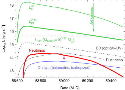
Our results are summarized in Fig. 6 here (luminosity evolution) and Fig. 2 in the main text (neutrino fluence as a function of energy). The neutrino lightcurve predicts an average delay similar to the actual delay, although the predicted variation is large. The buildup of the neutrino lightcurve is delayed with respect to the BB because of the size of the system delaying the buildup of the external target photons. On the other hand, the late-term decrease of the production/isotropization radius sightly boosts the neutrino production efficiency. It is intriguing that the shape of the isotropized X-ray curve is very similar to the dust echo curve in Fig. 2 (main text); suggesting that the dust might play a role in the X-ray isotropization.

In comparison to AT2019dsg, the main differences in the model are the larger size of the system, the larger SMBH mass and the smaller fraction of energy going into the jet, the larger mass of the disrupted star, and a higher assumed back-scattering efficiency, because the system is expected to be covered with components of the pre-existing AGN. Furthermore, a slightly higher $\Gamma$ (than AT2019dsg) was assumed and a viewing angle $\theta_{v}=1/\Gamma$, such that Doppler and Gamma factors are identical (for AT2019fdr). The neutrino event rates are relatively similar, and so are the spectra. Note that the origin of the X-ray isotropization might be different: for AT2019dsg, a mildly relativistic outflow – originally associated with the radio signal – was assumed to be the reason, since no pre-existing AGN components were expected. In the case of AT2019fdr, the scattering could also come from a similar outflow, but there is no observational evidence for that and there are the other possibilities discussed earlier. In all cases, the observed time delay of the neutrino seems to scale with the size of the system.

It has been established that relativistic jets lead to radio afterglow emission. In the case of AT2019dsg, the radio data are best explained by sub-relativistic winds in the standard leptonic emission scenario rather than a relativistic jet Mohan et al. (2022); Matsumoto et al. (2022). The origin of the radio emission from AT2019fdr is uncertain, and there is no evidence for a jet. In this regard, Murase et al. (2020) examined a hidden jet model by requiring that the relativistic jet is choked such that afterglow emission does not emerge. We do not consider this model here because of insufficient energetics to describe the neutrino event.

References

- Aartsen et al. (2017) M. G. Aartsen et al. (IceCube Collaboration), J. Instr. 12, P03012–P03012 (2017).
- Aartsen et al. (2015) M. G. Aartsen et al. (IceCube Collaboration), Phys. Rev. Lett. 115, 081102 (2015).
- Aartsen et al. (2014) M. G. Aartsen et al. (IceCube Collaboration), Phys. Rev. Lett. 113, 101101 (2014).
- Aartsen et al. (2013) M. Aartsen et al. (IceCube Collaboration), Science 342, 10.1126/science.1242856 (2013).
- Ahlers and Halzen (2018) M. Ahlers and F. Halzen, Prog. Part. Nuc. Phys. 102, 73 (2018).
- Kowalski (2021) M. Kowalski, Nat. Astron. 5, 732 (2021).
- Aartsen et al. (2018a) M. G. Aartsen et al. (IceCube Collaboration), Science 361, eaat1378 (2018a).
- Aartsen et al. (2018b) M. G. Aartsen et al. (IceCube Collaboration), Science 361, 147 (2018b).
- Garrappa et al. (2019) S. Garrappa et al. (Fermi LAT Collaboration), Astrophys. J. 880, 103 (2019).
- Stein et al. (2021a) R. Stein et al., Nat. Astron. 5, 510 (2021a).
- Aartsen et al. (2020) M. G. Aartsen et al. (IceCube Collaboration), Phys. Rev. Lett. 124, 10.1103/physrevlett.124.051103 (2020).
- Berezinsky (1977) V. S. Berezinsky, Proceedings of the International Conference “Neutrino ’77” (1977).
- Eichler (1979) D. Eichler, Astrophys. J. 232, 106 (1979).
- Stecker et al. (1991) F. W. Stecker, C. Done, M. H. Salamon, and P. Sommers, Phys. Rev. Lett. 66, 2697 (1991).
- Mannheim (1993) K. Mannheim, Astron. Astrophys. 269, 67 (1993).
- Szabo and Protheroe (1994) A. Szabo and R. Protheroe, Astropart. Phys. 2, 375 (1994).
- Murase (2017) K. Murase, Active galactic nuclei as high-energy neutrino sources, in Neutrino Astronomy (World Scientific, 2017) p. 15–31.
- Murase et al. (2016) K. Murase, D. Guetta, and M. Ahlers, Phys. Rev. Lett. 116, 071101 (2016).
- Palladino, Andrea and Winter, Walter (2018) Palladino, Andrea and Winter, Walter, Astron. Astrophys. 615, A168 (2018).
- Bartos et al. (2021) I. Bartos, D. Veske, M. Kowalski, Z. Márka, and S. Márka, Astrophys. J. 921, 45 (2021).
- Murase et al. (2020) K. Murase, S. S. Kimura, and P. Mészáros, Phys. Rev. Lett. 125, 011101 (2020).
- Farrar and Gruzinov (2009) G. R. Farrar and A. Gruzinov, Astrophys. J. 693, 329 (2009).
- Murase (2008) K. Murase, Gamma-ray bursts. Proceedings, Conference, Nanjing, P.R. China, June 23-27, 2008, AIP Conf. Proc. 1065, 201 (2008).
- Wang et al. (2011) X.-Y. Wang, R.-Y. Liu, Z.-G. Dai, and K. S. Cheng, Phys. Rev. D 84, 081301(R) (2011).
- (25) G. R. Farrar and T. Piran, arXiv:1411.0704 .
- Wang and Liu (2016) X.-Y. Wang and R.-Y. Liu, Phys. Rev. D 93, 083005 (2016).
- Dai and Fang (2017) L. Dai and K. Fang, Mon. Not. R. Astron. Soc. 469, 1354 (2017).
- Senno et al. (2017) N. Senno, K. Murase, and P. Mészáros, Astrophys. J. 838, 3 (2017).
- Guépin, Claire et al. (2018) Guépin, Claire, Kotera, Kumiko, Barausse, Enrico, Fang, Ke, and Murase, Kohta, Astron. Astrophys. 616, A179 (2018), [Erratum: Astron. Astrophys. 636, C3 (2020)].
- Lunardini and Winter (2017) C. Lunardini and W. Winter, Phys. Rev. D 95, 123001 (2017).
- Zhang et al. (2017) B. T. Zhang, K. Murase, F. Oikonomou, and Z. Li, Phys. Rev. D 96, 063007 (2017).
- Biehl et al. (2018) D. Biehl, D. Boncioli, C. Lunardini, and W. Winter, Sci. Rep. 8, 10828 (2018).
- Hayasaki and Yamazaki (2019) K. Hayasaki and R. Yamazaki, Astrophys. J. 886, 114 (2019).
- Winter and Lunardini (2021) W. Winter and C. Lunardini, Nat. Astron. 5, 472 (2021).
- Murase et al. (2020) K. Murase, S. S. Kimura, B. T. Zhang, F. Oikonomou, and M. Petropoulou, Astrophys. J. 902, 108 (2020).
- Liu et al. (2020) R.-Y. Liu, S.-Q. Xi, and X.-Y. Wang, Phys. Rev. D 102, 083028 (2020).
- Fang et al. (2020) K. Fang, B. D. Metzger, I. Vurm, E. Aydi, and L. Chomiuk, Astrophys. J. 904, 4 (2020).
- Winter and Lunardini (2021) W. Winter and C. Lunardini, Proc. Sci. ICRC2021, 997 (2021).
- Hayasaki (2021) K. Hayasaki, Nat. Astron. 5, 436 (2021).
- Cannizzaro et al. (2021) G. Cannizzaro et al., Mon. Not. R. Astron. Soc. 504, 792 (2021).
- Cendes et al. (2021) Y. Cendes, K. D. Alexander, E. Berger, T. Eftekhari, P. K. G. Williams, and R. Chornock, Astrophys. J. 919, 127 (2021).
- Mohan et al. (2022) P. Mohan, T. An, Y. Zhang, J. Yang, X. Yang, and A. Wang, Astrophys. J. 927, 74 (2022).
- Matsumoto et al. (2022) T. Matsumoto, T. Piran, and J. H. Krolik, Mon. Not. R. Astron. Soc. 511, 5085 (2022).
- Frederick et al. (2021) S. Frederick et al., Astrophys. J. 920, 56 (2021).
- Bellm et al. (2018) E. C. Bellm et al., Publ. Astron. Soc. Pac. 131, 018002 (2018).
- Graham et al. (2019) M. J. Graham et al., Publ. Astron. Soc. Pac. 131, 078001 (2019).
- Dekany et al. (2020) R. Dekany et al., Publ. Astron. Soc. Pac. 132, 038001 (2020).
- Stein (2020a) R. Stein, GCN Circ. 27865 (2020a).
- Stein et al. (2021b) R. Stein, S. Reusch, and J. Necker, nuztf: v2.2.1, https://github.com/desy-multimessenger/nuztf (2021b).
- Nordin, J. et al. (2019) Nordin, J. et al., Astron. Astrophys. 631, A147 (2019).
- Kowalski and Mohr (2007) M. Kowalski and A. Mohr, Astropart. Phys. 27, 533 (2007).
- Reusch et al. (2020a) S. Reusch, R. Stein, A. Franckowiak, and S. Gezari, GCN Circ. 27872 (2020a).
- Calzetti et al. (2000) D. Calzetti, L. Armus, R. C. Bohlin, A. L. Kinney, J. Koornneef, and T. Storchi-Bergmann, Astrophys. J. 533, 682 (2000).
- Nordin et al. (2019) J. Nordin, V. Brinnel, M. Giomi, J. V. Santen, A. Gal-Yam, O. Yaron, and S. Schulze, TNS Disc. Rep. 2019-771, 1 (2019).
- Law et al. (2009) N. M. Law et al., Publ. Astron. Soc. Pac. 121, 1395–1408 (2009).
- Gal-Yam (2019) A. Gal-Yam, Annu. Rev. Astron. Astrophys. 57, 305–333 (2019).
- Chornock et al. (2019) R. Chornock, P. K. Blanchard, S. Gomez, G. Hosseinzadeh, and E. Berger, TNS Class. Rep. 2019-1016, 1 (2019).
- Pitik et al. (2022) T. Pitik, I. Tamborra, C. R. Angus, and K. Auchettl, Astrophys. J. 929, 163 (2022).
- Roming et al. (2005) P. W. A. Roming et al., Space Sci. Rev. 120, 95 (2005).
- Gehrels et al. (2004) N. Gehrels et al., Astrophys. J. 611, 1005 (2004).
- Burrows et al. (2005) D. N. Burrows et al., Space Sci. Rev. 120, 165–195 (2005).
- Predehl, P. et al. (2021) Predehl, P. et al., Astron. Astrophys. 647, A1 (2021).
- Sunyaev et al. (2021) R. Sunyaev et al., Astron. Astrophys 656, A132 (2021).
- Saxton et al. (2020) R. Saxton, S. Komossa, K. Auchettl, and P. G. Jonker, Space Sci. Rev. 216, 85 (2020).
- Leighly (1999) K. M. Leighly, Astrophys. J. Suppl. Ser. 125, 317 (1999).
- Vaughan et al. (1999) S. Vaughan, J. Reeves, R. Warwick, and R. Edelson, Mon. Not. R. Astron. Soc. 309, 113 (1999).
- Margutti et al. (2018) R. Margutti et al., Astrophys. J. 864, 45 (2018).
- Barbary et al. (2008) K. Barbary et al., Astrophys. J. 690, 1358 (2008).
- Gänsicke et al. (2009) B. T. Gänsicke, A. J. Levan, T. R. Marsh, and P. J. Wheatley, Astrophys. J. 697, L129 (2009).
- Mainzer et al. (2011) A. Mainzer et al., Astrophys. J. 731, 53 (2011).
- Wright et al. (2010) E. L. Wright et al., Astron. J. 140, 1868–1881 (2010).
- Wilson et al. (2003) J. C. Wilson et al., in Instrument Design and Performance for Optical/Infrared Ground-based Telescopes, Society of Photo-Optical Instrumentation Engineers (SPIE) Conference Series, Vol. 4841, edited by M. Iye and A. F. M. Moorwood (2003) pp. 451–458.
- van Velzen et al. (2016) S. van Velzen, A. J. Mendez, J. H. Krolik, and V. Gorjian, Astrophys. J. 829, 19 (2016).
- Dong et al. (2016) S. Dong et al., Science 351, 257 (2016).
- Leloudas et al. (2016) G. Leloudas et al., Nat. Astron. 1, 0002 (2016).
- Kankare et al. (2017) E. Kankare et al., Nature Astronomy 1, 865 (2017).
- Kool et al. (2020) E. C. Kool et al., Mon. Not. R. Astron. Soc. 498, 2167 (2020).
- Mattila et al. (2018) S. Mattila et al., Science 361, 482 (2018).
- Perley et al. (2011) R. A. Perley, C. J. Chandler, B. J. Butler, and J. M. Wrobel, Astrophys. J. Lett. 739, L1 (2011).
- Atwood et al. (2009) W. B. Atwood et al., Astrophys. J. 697, 1071 (2009).
- (82) S. van Velzen et al., arXiv:2111.09391 .
- Strotjohann et al. (2019) N. L. Strotjohann, M. Kowalski, and A. Franckowiak, Astron. Astrophys. 622, L9 (2019).
- van Velzen et al. (2021) S. van Velzen et al., Astrophys. J. 908, 4 (2021).
- Blaufuss et al. (2019) E. Blaufuss, T. Kintscher, L. Lu, and C. F. Tung, Proc. Sci. ICRC2019, 1021 (2019).
- Jiang et al. (2019) Y.-F. Jiang, J. M. Stone, and S. W. Davis, Astrophys. J. 880, 67 (2019).
- Mummery (2021) A. Mummery, Mon. Not. R. Astron. Soc. 504, 5144 (2021).
- Ryu et al. (2020) T. Ryu, J. Krolik, and T. Piran, Astrophys. J. 904, 73 (2020).
- Chan et al. (2019) C.-H. Chan, T. Piran, J. H. Krolik, and D. Saban, Astrophys. J. 881, 113 (2019).
- Arcavi et al. (2014) I. Arcavi et al., Astrophys. J. 793, 38 (2014).
- French et al. (2020) K. D. French, T. Wevers, J. Law-Smith, O. Graur, and A. I. Zabludoff, Space Sci. Rev. 216, 32 (2020).
- Stone et al. (2018) N. C. Stone, A. Generozov, E. Vasiliev, and B. D. Metzger, Mon. Not. R. Astron. Soc. 480, 5060 (2018).
- IceCube Collaboration (2018) IceCube Collaboration, DOI:10.21234/B4F04V (2018).
- Albert et al. (2021) A. Albert et al. (ANTARES Collaboration), Astrophys. J. 920, 50 (2021).
- Reusch (2022) S. Reusch, at2019fdr: V1.0 release, https://github.com/simeonreusch/at2019fdr (2022).
- Rigault (2018) M. Rigault, ztfquery, a python tool to access ztf data, https://github.com/mickaelrigault/ztfquery (2018).
- Gaia Collaboration (2018) Gaia Collaboration, Astron. Astrophys. 616, A1 (2018).
- Ayala (2020) H. Ayala, GCN Circ. 27873 (2020).
- Savchenko (2020) V. Savchenko, GCN Circ. 27866 (2020).
- Sazonov et al. (2021) S. Sazonov et al., Mon. Not. R. Astron. Soc. , 3820 (2021).
- Ben Bekhti et al. (2016) N. Ben Bekhti et al. (HI4PI Collaboration), Astron. Astrophys. 594, A116 (2016).
- Centre (2020) U. S. S. D. Centre, Swift xrt data products generator, https://www.swift.ac.uk/user_objects (2020).
- Evans et al. (2009) P. A. Evans et al., Mon. Not. R. Astron. Soc. 397, 1177 (2009).
- Arida and Sabol (2020) M. Arida and E. Sabol, Heasarc webpimms, https://heasarc.gsfc.nasa.gov/cgi-bin/Tools/w3pimms/w3pimms.pl (2020).
- Reusch (2021) S. Reusch, ztffps: v1.0.3, https://github.com/simeonreusch/ztffps (2021).
- Rigault (2020) M. Rigault, ztflc, https://github.com/mickaelrigault/ztflc (2020).
- Breeveld et al. (2011) A. A. Breeveld, W. Landsman, S. T. Holland, P. Roming, N. P. M. Kuin, and M. J. Page, in American Institute of Physics Conference Series, American Institute of Physics Conference Series, Vol. 1358, edited by J. E. McEnery, J. L. Racusin, and N. Gehrels (2011) pp. 373–376.
- De et al. (2020) K. De et al., Publ. Astron. Soc. Pac. 132, 025001 (2020).
- Skrutskie et al. (2006) M. F. Skrutskie et al., Astron. J. 131, 1163 (2006).
- Peng et al. (2002) C. Y. Peng, L. C. Ho, C. D. Impey, and H.-W. Rix, Astron. J. 124, 266 (2002).
- Bradley et al. (2020) L. Bradley et al., astropy/photutils: 1.0.0, https://github.com/astropy/photutils (2020).
- York et al. (2000) D. G. York et al., Astrophys. J. 120, 1579 (2000).
- van Velzen et al. (2020) S. van Velzen, T. W. S. Holoien, F. Onori, T. Hung, and I. Arcavi, Space Sci. Rev. 216, 124 (2020).
- Martin et al. (2005) D. C. Martin et al., Astrophys. J. 619, L1 (2005).
- Million et al. (2016) C. Million, S. W. Fleming, B. Shiao, M. Seibert, P. Loyd, M. Tucker, M. Smith, R. Thompson, and R. L. White, Astrophys. J. 833, 292 (2016).
- Stoughton et al. (2002) C. Stoughton et al., Astron. J. 123, 485 (2002).
- Lawrence et al. (2007) A. Lawrence et al., Mon. Not. R. Astron. Soc. 379, 1599 (2007).
- Conroy and Gunn (2010) C. Conroy and J. E. Gunn, Astrophys. J. 712, 833 (2010).
- Foreman-Mackey et al. (2014) D. Foreman-Mackey, J. Sick, and B. Johnson, python-fsps: Python bindings to FSPS (v0.1.1) (2014).
- Jones et al. (2015) D. O. Jones, D. M. Scolnic, and S. A. Rodney, PythonPhot: Simple DAOPHOT-type photometry in Python (2015), ascl:1501.010 .
- Masci (2013) F. Masci, ICORE: Image Co-addition with Optional Resolution Enhancement (2013), ascl:1302.010 .
- Lacy et al. (2020) M. Lacy et al., Publ. Astron. Soc. Pac. 132, 035001 (2020).
- Barniol Duran et al. (2013) R. Barniol Duran, E. Nakar, and T. Piran, Astrophys. J. 772, 78 (2013).
- Morlino and Caprioli (2012) G. Morlino and D. Caprioli, Astron. Astrophys. 538, A81 (2012).
- Eftekhari et al. (2018) T. Eftekhari, E. Berger, B. A. Zauderer, R. Margutti, and K. D. Alexander, Astrophys. J. 854, 86 (2018).
- Horesh et al. (2013) A. Horesh et al., Mon. Not. R. Astron. Soc. 436, 1258 (2013).
- Generozov et al. (2017) A. Generozov, P. Mimica, B. D. Metzger, N. C. Stone, D. Giannios, and M. A. Aloy, Mon. Not. R. Astron. Soc. 464, 2481 (2017).
- Newville et al. (2021) M. Newville, T. Stensitzki, D. B. Allen, and A. Ingargiola, LMFIT: Non-Linear Least-Square Minimization and Curve-Fitting for Python (2021).
- Kyle (2016) B. Kyle, extinction, https://doi.org/10.5281/zenodo.804967 (2016).
- Vestergaard and Peterson (2006) M. Vestergaard and B. M. Peterson, Astrophys. J. 641, 689 (2006).
- Guo et al. (2018) H. Guo, Y. Shen, and S. Wang, PyQSOFit: Python code to fit the spectrum of quasars (2018), ascl:1809.008 .
- Fitzpatrick (1999) E. L. Fitzpatrick, Publ. Astron. Soc. Pac. 111, 63 (1999).
- Schlegel et al. (1998) D. J. Schlegel, D. P. Finkbeiner, and M. Davis, Astrophys. J. 500, 525 (1998).
- Boroson and Green (1992) T. A. Boroson and R. F. Green, Astrophys. J. Suppl. Ser. 80, 109 (1992).
- Shen et al. (2011) Y. Shen et al., Astrophys. J. Suppl. Ser. 194, 45 (2011).
- Guo et al. (2019) H. Guo, X. Liu, Y. Shen, A. Loeb, T. Monroe, and J. X. Prochaska, Mon. Not. R. Astron. Soc. 482, 3288 (2019).
- Shen et al. (2019) Y. Shen et al., Astrophys. J. , Suppl. Ser. 241, 34 (2019).
- McLure and Dunlop (2002) R. J. McLure and J. S. Dunlop, Mon. Not. R. Astron. Soc. 331, 795 (2002).
- Patterson et al. (2019) M. T. Patterson, E. C. Bellm, B. Rusholme, F. J. Masci, M. Juric, K. S. Krughoff, V. Z. Golkhou, M. J. Graham, S. R. Kulkarni, and G. Helou, Publ. Astron. Soc. Pac. 131, 018001 (2019).
- Masci et al. (2019) F. J. Masci et al., Publ. Astron. Soc. Pac. 131, 018003 (2019).
- Blaufuss (2019a) E. Blaufuss, GCN Circ. 24378 (2019a).
- Stein et al. (2019a) R. Stein, A. Franckowiak, J. van Santen, L. Rauch, M. M. Kasliwal, I. Andreoni, T. Ahumada, M. Coughlin, L. P. Singer, and S. Anand, The Astronomer’s Telegram 12730, 1 (2019a).
- Blaufuss (2019b) E. Blaufuss, GCN Circ. 24910 (2019b).
- Stein et al. (2019b) R. Stein et al., The Astronomer’s Telegram 12879, 1 (2019b).
- Stein (2019a) R. Stein, GCN Circ. 25225 (2019a).
- Stein et al. (2019c) R. Stein, A. Franckowiak, M. M. Kasliwal, I. Andreoni, M. Coughlin, L. P. Singer, F. Masci, and S. van Velzen, The Astronomer’s Telegram 12974, 1 (2019c).
- Blaufuss (2019c) E. Blaufuss, GCN Circ. 25806 (2019c).
- Stein et al. (2019d) R. Stein, A. Franckowiak, M. Kowalski, and M. Kasliwal, The Astronomer’s Telegram 13125, 1 (2019d).
- Stein et al. (2019e) R. Stein, A. Franckowiak, M. Kowalski, and M. Kasliwal, GCN Circ. 25824 (2019e).
- Stein (2019b) R. Stein, GCN Circ. 25913 (2019b).
- Stein et al. (2019f) R. Stein, A. Franckowiak, J. Necker, S. Gezari, and S. v. Velzen, The Astronomer’s Telegram 13160, 1 (2019f).
- Stein et al. (2019g) R. Stein, A. Franckowiak, J. Necker, S. Gezari, and S. van Velzen, GCN Circ. 25929 (2019g).
- Stein (2020b) R. Stein, GCN Circ. 26655 (2020b).
- Stein and Reusch (2020) R. Stein and S. Reusch, GCN Circ. 26667 (2020).
- Stein (2020c) R. Stein, GCN Circ. 26696 (2020c).
- Reusch and Stein (2020a) S. Reusch and R. Stein, GCN Circ. 26747 (2020a).
- Lagunas Gualda (2020a) C. Lagunas Gualda, GCN Circ. 26802 (2020a).
- Reusch and Stein (2020b) S. Reusch and R. Stein, GCN Circ. 26813 (2020b).
- Reusch and Stein (2020c) S. Reusch and R. Stein, GCN Circ. 26816 (2020c).
- Lagunas Gualda (2020b) C. Lagunas Gualda, GCN Circ. 27719 (2020b).
- Reusch et al. (2020b) S. Reusch, R. Stein, and A. Franckowiak, GCN Circ. 27721 (2020b).
- Stein (2020d) R. Stein, GCN Circ. 27865 (2020d).
- Reusch et al. (2020c) S. Reusch, R. Stein, A. Franckowiak, and S. Gezari, GCN Circ. 27872 (2020c).
- Reusch et al. (2020d) S. Reusch, R. Stein, A. Franckowiak, J. Sollerman, T. Schweyer, and C. Barbarino, GCN Circ. 27910 (2020d).
- Reusch et al. (2020e) S. Reusch, R. Stein, A. Franckowiak, J. Necker, J. Sollerman, C. Barbarino, and T. Schweyer, GCN Circ. 27980 (2020e).
- Santander (2020a) M. Santander, GCN Circ. 27997 (2020a).
- Reusch et al. (2020f) S. Reusch, R. Stein, and A. Franckowiak, GCN Circ. 28005 (2020f).
- Blaufuss (2020a) E. Blaufuss, GCN Circ. 28433 (2020a).
- Reusch et al. (2020g) S. Reusch, R. Stein, A. Franckowiak, I. Andreoni, and M. Coughlin, GCN Circ. 28441 (2020g).
- Reusch et al. (2020h) S. Reusch, R. Stein, A. Franckowiak, S. Schulze, and J. Sollerman, GCN Circ. 28465 (2020h).
- Lagunas Gualda (2020c) C. Lagunas Gualda, GCN Circ. 28504 (2020c).
- Reusch et al. (2020i) S. Reusch, R. Stein, S. Weimann, and A. Franckowiak, GCN Circ. 28520 (2020i).
- Lagunas Gualda (2020d) C. Lagunas Gualda, GCN Circ. 28532 (2020d).
- Weimann et al. (2020a) S. Weimann, R. Stein, S. Reusch, and A. Franckowiak, GCN Circ. 28551 (2020a).
- Santander (2020b) M. Santander, GCN Circ. 28575 (2020b).
- Reusch et al. (2020j) S. Reusch, S. Weimann, R. Stein, and A. Franckowiak, GCN Circ. 28609 (2020j).
- Lagunas Gualda (2020e) C. Lagunas Gualda, GCN Circ. 28715 (2020e).
- Stein et al. (2020a) R. Stein, S. Reusch, S. Weimann, and M. Coughlin, GCN Circ. 28757, 1 (2020a).
- Lagunas Gualda (2020f) C. Lagunas Gualda, GCN Circ. 28969 (2020f).
- Weimann et al. (2020b) S. Weimann, R. Stein, S. Reusch, and A. Franckowiak, GCN Circ. 28989, 1 (2020b).
- Lagunas Gualda (2020g) C. Lagunas Gualda, GCN Circ. 29012 (2020g).
- Reusch et al. (2020k) S. Reusch, S. Weimann, R. Stein, and A. Franckowiak, GCN Circ. 29031 (2020k).
- Blaufuss (2020b) E. Blaufuss, GCN Circ. 29120 (2020b).
- Stein et al. (2020b) R. Stein, S. Weimann, S. Reusch, and A. Franckowiak, GCN Circ. 29172 (2020b).
- Lagunas Gualda (2021) C. Lagunas Gualda, GCN Circ. 29454 (2021).
- Reusch et al. (2021) S. Reusch, S. Weimann, R. Stein, M. Coughlin, and A. Franckowiak, GCN Circ. 29461 (2021).
- Santander (2021a) M. Santander, GCN Circ. 29976 (2021a).
- Stein et al. (2021a) R. Stein, S. Weimann, J. Necker, S. Reusch, and A. Franckowiak, GCN Circ. 29999 (2021a).
- Santander (2021b) M. Santander, GCN Circ. 30342 (2021b).
- Necker et al. (2021) J. Necker, R. Stein, S. Weimann, S. Reusch, and A. Franckowiak, GCN Circ. 30349 (2021).
- Santander (2021c) M. Santander, GCN Circ. 30627 (2021c).
- Stein et al. (2021b) R. Stein, S. Weimann, S. Reusch, J. Necker, A. Franckowiak, and M. Coughlin, GCN Circ. 30644 (2021b).
- Lincetto (2021) M. Lincetto, GCN Circ. 30862 (2021).
- Weimann et al. (2021) S. Weimann, S. Reusch, J. Necker, R. Stein, and A. Franckowiak, GCN Circ. 30870 (2021).
- Kimura et al. (2015) S. S. Kimura, K. Murase, and K. Toma, Astrophys. J. 806, 159 (2015).
- McKinney et al. (2015) J. C. McKinney, L. Dai, and M. J. Avara, Mon. Not. R. Astron. Soc. 454, L6 (2015).
- Takeo et al. (2019) E. Takeo, K. Inayoshi, K. Ohsuga, H. R. Takahashi, and S. Mineshige, Mon. Not. R. Astron. Soc. 488, 2689 (2019).
- Mücke et al. (2000) A. Mücke, R. Engel, J. P. Rachen, R. J. Protheroe, and T. Stanev, Computer Phys. Comm. 124, 290 (2000).
- Io and Suzuki (2014) Y. Io and T. K. Suzuki, Astrophys. J. 780, 46 (2014).
- Jiang et al. (2014) Y.-F. Jiang, J. M. Stone, and S. W. Davis, Astrophys. J. 784, 169 (2014).
- Takahashi et al. (2016) H. R. Takahashi, K. Ohsuga, T. Kawashima, and Y. Sekiguchi, Astrophys. J. 826, 23 (2016).
- Strubbe and Quataert (2009) L. E. Strubbe and E. Quataert, Mon. Not. R. Astron. Soc. 400, 2070 (2009).
- Miller (2015) M. C. Miller, Astrophys. J. 805, 83 (2015).
- Metzger and Stone (2016) B. D. Metzger and N. C. Stone, Mon. Not. R. Astron. Soc. 461, 948 (2016).
- Dai et al. (2018) L. Dai, J. C. McKinney, N. Roth, E. Ramirez-Ruiz, and M. C. Miller, Astrophys. J. 859, L20 (2018).
- Mummery and Balbus (2021a) A. Mummery and S. A. Balbus, Mon. Not. R. Astron. Soc. 504, 4730 (2021a).
- (207) A. Mummery, arXiv:2104.06212 .
- Mummery and Balbus (2021b) A. Mummery and S. A. Balbus, Mon. Not. R. Astron. Soc. 505, 1629 (2021b).
- Kochanek (2016) C. S. Kochanek, Mon. Not. R. Astron. Soc. 461, 371 (2016).
- Rees (1988) M. J. Rees, Nature 333, 523 (1988).
- De Colle et al. (2012) F. De Colle, J. Guillochon, J. Naiman, and E. Ramirez-Ruiz, Astrophys. J. 760, 103 (2012).
- Murase et al. (2014) K. Murase, Y. Inoue, and C. D. Dermer, Phys. Rev. D 90, 023007 (2014).