Bivariate Chromatic Polynomials of Mixed Graphs

Abstract

The bivariate chromatic polynomial $\chi_{G}(x,y)$ of a graph $G=(V,E)$, introduced by Dohmen–Pönitz–Tittmann (2003), counts all $x$-colorings of $G$ such that adjacent vertices get different colors if they are $\leq y$. We extend this notion to mixed graphs, which have both directed and undirected edges. Our main result is a decomposition formula which expresses $\chi_{G}(x,y)$ as a sum of bivariate order polynomials (Beck–Farahmand–Karunaratne–Zuniga Ruiz 2020), and a combinatorial reciprocity theorem for $\chi_{G}(x,y)$.

1 Introduction

Graph coloring problems are ubiquitous in many areas within and outside of mathematics. Our interest is in enumerating proper colorings for graphs, directed graphs, and mixed graphs (and in the latter two instances, there are two definitions of the notion of a coloring being proper).

The motivation of our study is the bivariate chromatic polynomial $\chi_{G}(x,y)$ of a graph $G=(V,E)$, first introduced in Dohmen et al. (2003) and defined as the counting function of colorings $c:V\to[x]:=\left\{1,2,\dots,x\right\}$ that satisfy for any edge $vw\in E$

$$c(v)\neq c(w)\quad\text{ or }\quad c(v)=c(w)>y\,.$$

The usual univariate chromatic polynomial of $G$ can be recovered as the special evaluation $\chi_{G}(x,x)$. Dohmen, Pönitz, and Tittmann provided basic properties of $\chi_{G}(x,y)$ in Dohmen et al. (2003), including polynomiality and special evaluations which yield the matching and independence polynomials of $G$. Subsequent results include a deletion–contraction formula and applications to Fibonacci-sequence identities Hillar and Windfeldt (2008/09), common generalizations of $\chi_{G}(x,y)$ and the Tutte polynomial Averbouch et al. (2010), and closed formulas for paths and cycles Dohmen (2015).

We initiate the study of a directed/mixed version of this bivariate chromatic polynomial. Since directed graphs form a subset of mixed graphs, we may restrict our definitions to a mixed graph $G=(V,E,A)$ consisting, as usual, of a set $V$ of vertices, a set $E$ of (undirected) edges, and a set $A$ of arcs (directed edges). Coloring problems in mixed graphs have various applications, for example in scheduling problems in which one has both disjunctive and precedence constraints (see, e.g., Furmańczyk et al. (2009); Hansen et al. (1997); Sotskov et al. (2002)).

Definition.

For a mixed graph $G=\left(V,E,A\right)$, the bivariate chromatic polynomial $\chi_{G}(x,y)$, where $1\leq y\leq x$, is defined as the counting function of colorings $c:V\longrightarrow\left[x\right]$ that satisfies for every edge $uv\in E$

$$c(u)\neq c(v)\quad \text{ or }\quad c(u)>y$$ (1)

and for every arc $\overrightarrow{uv}\in A$

$$c(u)<c(v)\quad \text{ or }\quad c(u)>y\,.$$ (2)

It is not obvious that this counting function is a polynomial in $x$ and $y$; we will prove this as a by-product of Theorem 1 below. Naturally, for a mixed graph with $A=\emptyset$, we recover the Dohmen–Pönitz–Tittmann chromatic polynomial above. On the other hand, $\chi_{G}(x,x)$ is the univariate chromatic polynomial of the mixed graph $G$; Sotskov and Tanaev (1976) showed that this function (if not identically zero) is indeed a polynomial in $x$ of degree $|V|$ and computed the two leading coefficients. We note that $\chi_{G}(x,x)$ is sometimes called the strong chromatic polynomial of $G$, because there is an alternative notion of a proper coloring of $G$ in which the inequality in (2) is replaced by $\leq$ (see, e.g., Kotek et al. (2008)).

Example 1.

Consider the directed graph with $V=\left\{u,v\right\},$ $E=\emptyset$, $A=\left\{\overrightarrow{uv}\right\}$. A quick case analysis yields the bivariate chromatic polynomial

$$\chi_{G}(x,y) ={x\choose 2}+y(x-y)+{x-y+1\choose 2}=\frac{1}{2}\left(2x^{2}-y^{2}-y\right).$$

Figure 1: A mixed graph $G$.

Example 2.

The mixed graph in Figure 1 has bivariate chromatic polynomial

$$\chi_{G}(x,y)=x^{3}-\frac{1}{2}xy^{2}-\frac{5}{2}xy+y^{2}+y$$

as we will compute in Section 4.

After providing some background in Section 2, we derive in Section 3 deletion–contraction formulas for $\chi_{G}(x,y)$. Our main results are in Section 4, where we decompose $\chi_{G}(x,y)$ into bivariate order polynomials (originally introduced in Beck et al. (2020) and loosely connected with the marked poset concepts of Ardila et al. (2011)), and Section 5, where we give a combinatorial reciprocity theorem interpreting $\chi_{G}(-x,-y)$. Our results recover known theorems for undirected graphs (the case $A=\emptyset$) Beck et al. (2020). Bivariate order polynomials are the natural counterparts of bivariate chromatic polynomials in the theory of posets. Our work reveals that bivariate order polynomials are as helpful in the setting of mixed graphs as they are for undirected graphs.

2 Chromatic and (Bicolored) Order Polynomials

For a finite poset $(P,\preceq)$, Stanley (1970) (see also (Stanley, 2012, Chapter 3)) famously introduced the “chromatic-like” order polynomial $\Omega_{P}(x)$ counting all order preserving maps $\varphi:P\to[x]$, that is,

$$a\preceq b\qquad\Longrightarrow\qquad\varphi(a)\leq\varphi(b)\,.$$

Here we think of $[x]$ as a chain with $x$ elements, and so $\leq$ denotes the usual order in $\mathbb{R}$. The connection to chromatic polynomials is best exhibited through a variant of $\Omega_{P}(x)$, namely the number $\Omega_{P}^{\circ}(x)$ of all strictly order preserving maps $\varphi:P\to[x]$:

$$a\prec b\qquad\Longrightarrow\qquad\varphi(a)<\varphi(b)\,.$$

When thinking of $P$ as an acyclic directed graph, it is a short step interpreting $\Omega_{P}^{\circ}(x)$ as a directed version of the chromatic polynomial. Along the same lines, one can write the chromatic polynomial of a given graph $G$ as

$$\chi_{G}(x)\ =\sum_{\sigma\text{ acyclic orientation of }G}\Omega_{\sigma}^{\circ}(x)\,.$$ (3)

Stanley’s two main initial results on order polynomials were

• decomposition formulas for $\Omega_{P}(x)$ and $\Omega_{P}^{\circ}(x)$ in terms of certain permutation statistics for linear extensions of $P$, from which polynomiality of $\Omega_{P}(x)$ and $\Omega_{P}^{\circ}(x)$ also follows;

• the combinatorial reciprocity theorem $(-1)^{|P|}\,\Omega_{P}(-x)\ =\ \Omega_{P}^{\circ}(x)\,.$

The latter, combined with (3), gives in turn rise to

• Stanley’s reciprocity theorem for chromatic polynomials: $(-1)^{|V|}\,\chi_{G}(-x)$ equals the number of pairs of an $x$-coloring and a compatible acyclic orientation Stanley (1973).

Reciprocity theorems for the two versions of univariate chromatic polynomials of mixed graphs were proved in Beck et al. (2012, 2015).

It is natural to extend order polynomials and the three bullet points above to the bivariate chromatic setting, and this was done for (undirected) graphs in Beck et al. (2020). As we will need it below, we recall the setup here. The finite poset $\left(P,\preceq\right)$ is called a bicolored poset if $P$ can be viewed as the disjoint union of sets $C$ and $S$, whose elements are called celeste and silver, respectively. This color labeling of the elements of the bicolored poset is captured in the order preserving maps by introducing another variable, as follows. A map $\varphi:P\longrightarrow\left[x\right]$ is called an order preserving $(x,y)$-map if

$$a\preceq b\ \Longrightarrow\ \varphi(a)\leq\varphi(b)\ \ \text{ for all }a,b\in P\qquad\text{ and }\qquad\varphi(c)\geq y\ \ \text{ for all }c\in C\,.$$

The function $\Omega_{P,\,C}(x,y)$ counts the number of order preserving $(x,y)$-maps. The map $\varphi:P\longrightarrow\left[x\right]$ is a strictly order preserving $(x,y)$-map if

$$a\prec b\ \Longrightarrow\ \varphi(a)<\varphi(b)\ \ \text{ for all }a,b\in P\qquad\text{ and }\qquad\varphi(c)>y\ \ \text{ for all }c\in C\,.$$

The function $\Omega^{\circ}_{P,\,C}(x,y)$ counts the number of strictly order preserving $(x,y)$-maps. The functions $\Omega^{\circ}_{P,\,C}(x,y)$ and $\Omega_{P,\,C}(x,y)$ are called bivariate order polynomial and weak bivariate order polynomial, respectively. They are indeed polynomials, which can be computed via certain descent statistics, and which are related via the combinatorial reciprocity Beck et al. (2020)

$$(-1)^{|P|}\,\Omega^{\circ}_{P,\,C}(-x,-y)\ =\ \Omega_{P,\,C}(x,y+1)\,.$$ (4)

As we mentioned in the introduction, bivariate order polynomials exhibit a connection to the theory of marked posets introduced in Ardila et al. (2011). Briefly, one marks here the celeste elements, with a lower bound of $y$, and demands the lower bound 0 and the upper bound $x$ throughout the poset.

3 Deletion–Contraction

We start developing the properties of $\chi_{G}(x,y)$ by providing deletion–contraction formulas. For a mixed graph $G=\left(V,E,A\right)$, let $G-e$ denote edge deletion and $G/e$ denote edge contraction for an edge $e$ of $G$; let $v_{e}$ denote the vertex obtained after the contraction of edge $e$. We use a similar terminology for deleting/contracting an arc. For an arc $a$ of mixed graph $G$, let $G_{a}\coloneqq\left(V,E,A-\left\{\overrightarrow{uv}\right\}\cup\left\{\overrightarrow{vu}\right\}\right)$, that is, $G_{a}$ is the graph obtained by reversing the direction of arc $a$.

Proposition 1.

If $G=\left(V,E,A\right)$ is a mixed graph and $e\in E$ is an edge, then

$$\chi_{G}(x,y)\ =\ \chi_{G-e}(x,y)-\chi_{G/e}(x,y)+(x-y)\chi_{(G/e)-v_{e}}(x,y)\,.$$ (5)

If $a=\overrightarrow{uv}\in A$ is an arc, then

$$\begin{split}\chi_{G}(x,y)+\chi_{G_{a}}(x,y)\ &=\ \chi_{G-a}(x,y)-\chi_{G/a}(x,y)+(x-y)(1-x+y)\chi_{(G/a)-v_{a}}(x,y)\\ &\hskip 15.0pt+(x-y)\left(\chi_{G-a-v}(x,y)+\chi_{G-a-u}(x,y)\right).\end{split}$$ (6)

We remark that (5) is equivalent to (Averbouch et al., 2008, Proposition 1).

of (6).

Given $a=\overrightarrow{uv}\in A$, let $C$ be the set of all bivariate colorings of $G$ and $C_{a}$ the set of all bivariate colorings of $G_{a}$. By inclusion–exclusion,

$$\chi_{G}(x,y)+\chi_{G_{a}}(x,y) =\lvert C\cup C_{a}\rvert+\lvert C\cap C_{a}\rvert.$$ (7)

For a coloring $c\in C\cup C_{a}$, we count the number of ways the following coloring conditions are satisfied: $c(u)<c(v)$ or $c(v)<c(u)$ or $c(u)>y$ or $c(v)>y$. This means, we have to count the number of ways of coloring vertices $u$ and $v$ such that they can have any color labels from the set $\left\{1,2,\ldots,x\right\}$ except that the vertices can not have equal colors with labels in the set $\left\{1,2,\ldots,y\right\}$. This is exactly counted by

$$\chi_{G-a}(x,y)-\chi_{G/a}(x,y)+(x-y)\,\chi_{(G/a)-v_{a}}(x,y)\ =\ \lvert C\cup C_{a}\rvert\,.$$ (8)

For a coloring $c\in C\cap C_{a}$ we distinguish between the following cases..

• Case 1: $c(u)<c(v)$ and $c(u)>c(v)$.
  There does not exist a feasible coloring in $C\cap C_{a}$ that satisfies these conditions simultaneously.

• Case 2: $y<c(v)$ with $c(u)\leq c(v)$ and $y<c(u)$ with $c(v)\leq c(u)$.
  This implies the coloring condition $y<c(u)=c(v)$, which is counted in $(x-y)\,\chi_{(G/a)-v_{a}}(x,y)$ ways.

• Case 3: $c(u)<c(v)$ and $y<c(v)$ with $c(u)\leq c(v)$
  This implies that the coloring $c$ must satisfy $y<c(v)$ with $c(u)<c(v)$. There are two possibilities:

  • $y<c(u)<c(v)\leq x$.

    The colors for $u$ and $v$ can be chosen in ${x-y\choose 2}$ ways. Thus the number of possible colorings is ${x-y\choose 2}\chi_{(G/a)-v_{a}}(x,y)$.

  • $1\leq c(u)\leq y<c(v)\leq x$.

    There are $(x-y)$ ways to color $v$. To color $u$, the condition $1\leq c(u)\leq y$ needs to be satisfied. This is equivalent to counting colorings where $c(u)\leq x$ and removing the possible colorings with $c(u)>y$, giving $(x-y)\left(\chi_{G-a-u}(x,y)-(x-y)\chi_{(G/a)-v_{a}}(x,y)\right)$ colorings .

  In total there are ${x-y\choose 2}\chi_{(G/a)-v_{a}}(x,y)+(x-y)\big{(}\chi_{G-a-u}(x,y)-(x-y)\,\chi_{(G/a)-v_{a}}(x,y)\big{)}$ colorings.

• Case 4: $c(v)<c(u)$ and $y<c(u)$ with $c(v)\leq c(u)$
  This implies that the coloring $c$ must satisfy $y<c(u)$ with $c(v)<c(u)$. There are two possibilities:

  • $y<c(v)<c(u)\leq x$.

    The colors for $u$ and $v$ can be chosen in ${x-y\choose 2}$ ways. Thus the possible colorings are counted by ${x-y\choose 2}\chi_{(G/a)-v_{a}}(x,y)$.

  • $1\leq c(v)\leq y<c(u)\leq x$.

    There are $(x-y)$ ways to color $u$. For coloring $v$, the condition $1\leq c(v)\leq y$ needs to be satisfied. This is equivalent to counting colorings where $c(v)\leq x$ and removing the possible colorings with $c(v)>y$, yielding $(x-y)\left(\chi_{G-a-v}(x,y)-(x-y)\chi_{(G/a)-v_{a}}(x,y)\right)$ colorings.

  In total there are

  $${x-y\choose 2}\chi_{(G/a)-v_{a}}(x,y)+(x-y)\big{(}\chi_{G-a-v}(x,y)-(x-y)\,\chi_{(G/a)-v_{a}}(x,y)\big{)}$$

  colorings.

Thus

$$|C\cap C_{a}|\ =\ (x-y)\,\chi_{(G/a)-v_{a}}(x,y)+2{x-y\choose 2}\chi_{(G/a)-v_{a}}(x,y)$$

$$\qquad+(x-y)\left[\chi_{G-a-v}(x,y)-(x-y)\chi_{G/a-v}(x,y)\right]$$

$$\qquad+(x-y)\left[\chi_{G-a-u}(x,y)-(x-y)\chi_{G/a-u}(x,y)\right].$$ (9)

From Equations (7), (8) and (9) we finally obtain

$$\chi_{G}(x,y)+\chi_{G_{a}}(x,y)\ =\ \chi_{G-a}(x,y)-\chi_{G/a}(x,y)+(x-y)(1-x+y)\chi_{(G/a)-v_{a}}(x,y)$$

$$\hskip 15.0pt+(x-y)\left[\chi_{G-a-v}(x,y)+\chi_{G-a-u}(x,y)\right].\qed$$

4 Decomposition into Order Polynomials

For a mixed graph $G=\left(V,E,A\right)$, we recall that a flat of $G$ is a mixed graph $H$ that can be constructed from $G$ by a series of contractions of edges and arcs. We denote the sets of vertices, edges and arcs of the flat $H$ by $V(H),E(H)$ and $A(H)$, respectively. The subset of vertices of $H$ that results from contractions of $G$ is denoted by $C(H)$. An example is depicted in Figure 2, where we obtain the flat $H$ by contracting the edge $v_{1}v_{4}$. For this flat, the set of contracted vertices is $C(H)=\{v_{1}v_{4}\}$.

For a mixed graph $G$, let $G^{u}$ denote the underlying undirected graph, that is, the graph obtained from $G$ by replacing its arcs with undirected edges. For some acyclic orientation $\sigma$ of $G^{u}$, let $T(\sigma)$ be the set of all tail vertices of arcs $a$ of a flat $H$ of $G$ for which the orientation of an edge in $\sigma$ is opposite to the direction of $a$.

(a) A mixed graph $G$.

(b) The flat $H$ obtained by contracting the edge $v_{1}v_{4}$.

(c) The underlying undirected graph.

Figure 2: A mixed graph, one of its flat and the associated undirected graph.

Theorem 1.

For a mixed graph $G$,

$$\chi_{G}(x,y)\ =\sum_{H\text{ flat of }G}\sum_{\begin{subarray}{c}\sigma\text{ acyclic}\\ \text{orientation of }H^{u}\end{subarray}}\!\!\!\!\Omega^{\circ}_{\sigma,\,C(H)\cup T(\sigma)}(x,y)\,.$$

Note that this implies that $\chi_{G}(x,y)$ is a polynomial (because $\Omega^{\circ}_{\sigma,\,C(H)\cup T(\sigma)}(x,y)$ is).

Proof.

Let $c:V\longrightarrow[x]$ be a coloring of the mixed graph $G$ that satisfies the coloring conditions (1) and (2). Note that the colors of the end-points of edges and arcs can be equal only if they are $>y$. Let $H$ be a flat of $G$ obtained by contracting all edges and arcs whose end-points have the same color. Thus the vertices in $C(H)$ have color labels $>y$.

Consider $H^{u}$, the underlying undirected graph of the flat $H$. We orient the edges of $H^{u}$ along the color gradient, that is, for the edge $uv$, we introduce the orientation $u\longrightarrow v$ if and only if $c(u)<c(v)$. Let $\sigma$ be such an orientation. No two vertices in $H^{u}$ that are connected by an edge have identical color labels. This gives us that $\sigma$ is acyclic. Let

$$T(\sigma)\ \coloneqq\ \left\{v\in V(H):\,\overrightarrow{vw}\in A(H)\ \text{ and }\ v\longleftarrow w\ \text{ in }\ \sigma\right\}.$$

As the color gradient is decreasing along the arcs with tail vertices in the set $T(\sigma)$, we have $c(u)>y$ for each $u\in T(\sigma)$ from the coloring constraints. Now we regard the acyclic orientation $\sigma$ as a binary relation on the set $V(H^{u})$ defined by $u\preceq v$ if $u\longrightarrow v$. This gives us a bicolored poset $P$ where the vertices in the set $C(H)\cup T(\sigma)$ are celeste elements. The coloring $c$ is an order preserving $(x,y)$–map on $P$. The bivariate order polynomial $\Omega^{\circ}_{\sigma,\,C(H)\cup T(\sigma)}(x,y)$ counts all such order preserving maps.

Conversely, given a flat $H$ of $G$ and an acyclic orientation $\sigma$ of $H^{u}$, an order preserving $(x,y)$–map counted by $\Omega^{\circ}_{\sigma,\,C(H)\cup T(\sigma)}(x,y)$ can be extended to a coloring of $G$ as follows. All the vertices of $H$ get colors such that the color gradient follows $\sigma$. The celeste elements of the bicolored poset induced by the orientation $\sigma$ is given by the set $C(H)\cup T(\sigma)$. Hence the vertices in the set $T(\sigma)$ get colors $>y$. The coloring is then extended to the graph $G$ such that the vertices of the graph $G$ that result in contractions to form the flat $H$ get equal colors $>y$. This gives a coloring of the mixed graph $G$.

Consider two distinct colorings $c_{1}$ and $c_{2}$ of $G$. We need to show that the corresponding order preserving maps $\phi_{1}$ and $\phi_{2}$ are distinct.

Construct the flats $H_{1}$ and $H_{2}$ of the graph by contracting those edges and arcs that have end-vertices with equal color labels with respect to the colorings $c_{1}$ and $c_{2}$ respectively. If $H_{1}\neq H_{2}$, then the posets on the vertices of the underlying undirected graphs $H_{1}^{u}$ and $H_{2}^{u}$ will be different for each coloring. This will give us distinct order preserving $(x,y)$-maps.

Suppose $H_{1}=H_{2}$, that is, both flats are identical, then the underlying undirected graphs $H_{1}^{u}$ and $H_{2}^{u}$ will also be identical. Let $\sigma_{1}$ and $\sigma_{2}$ be acyclic orientations of $H_{1}^{u}$ and $H_{2}^{u}$, respectively.

Now define $T_{i}(\sigma_{i})\coloneqq\left\{v\in V(H_{i})\mid\overrightarrow{vw}\in A(H_{i})\text{ and }v\longleftarrow w\text{ in }\sigma_{i}\text{ of }H_{i}^{u}\right\}$ for $i=1,2$. If these sets are distinct, then the celeste elements in the corresponding bicolored posets will be distinct, resulting in different vertex orderings which will give distinct order preserving $(x,y)$–maps for corresponding colorings.

If for the vertex sets, $T_{1}(\sigma_{1})=T_{2}(\sigma_{2})$ but the acyclic orientations $\sigma_{1}$ and $\sigma_{2}$ are distinct, then the posets induced by these acyclic orientations will be distinct resulting in distinct order preserving $(x,y)$–maps for corresponding graph colorings.

If the flats, the acyclic orientation and the celeste sets are identical, then the bicolored posets corresponding to both colorings are the same. The bivariate order polynomial $\Omega^{\circ}_{\sigma,\,C(H)\cup T(\sigma)}(x,y)$ counts all possible order preserving $(x,y)$–maps on this bicolored poset exactly once. ∎

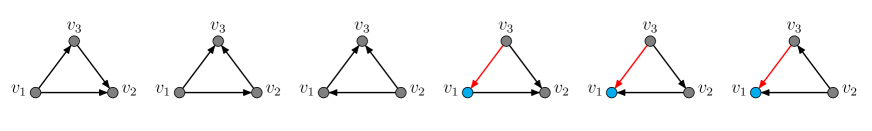
Figure 3: Acyclic orientations of contractions of $G$.

Naturally, an undirected graph is a special case of the above with $A=\emptyset$, and Theorem 1 specializes to one of the results of Beck et al. (2020):

Corollary 1.

For an undirected graph $G=\left(V,E\right)$,

$$\chi_{G}(x,y) =\sum_{H\text{ flat of }G\hskip 3.0pt}\sum_{\begin{subarray}{c}\sigma\text{ acyclic}\\ \text{orientation of }H\end{subarray}}\!\!\!\!\Omega^{\circ}_{\sigma,\,C(H)}(x,y)\,.$$

Example 3.

For the mixed graph $G$ shown in Figure 1, our proof of Theorem 1 is illustrated by Figure 3.

For $H=G$, there are six acyclic orientations of $H^{u}$ as shown in Figure 3.

There are three flats obtained by contracting one edge or one arc in $G$. For each underlying undirected graph of a flat, there are two acyclic orientations each. Figure 3 also shows these orientations. There is one flat obtained by contracting two edges or an edge and an arc of the graph resulting in a vertex $v_{1}v_{2}v_{3}$.

Computing the bivariate order polynomial for each of these orientations yields

$$\chi_{G}(x,y)\ =\ 3{x\choose 3}+2(x-y){y\choose 2}+(3y+6){x-y\choose 2}+3{x-y\choose 3}+(x-y)(3y+1)$$

$$=\ x^{3}-\frac{1}{2}xy^{2}-\frac{5}{2}xy+y^{2}+y\,.$$

5 Reciprocity

An orientation $\sigma$ and a coloring $c:V\longrightarrow[x]$ of the mixed graph $G$ satisfying (1) and (2) are compatible if $c(u)\leq c(v)$ for any edge/arc directed from $u$ to $v$ in $\sigma$.

We define $m_{H}(x,y)$ to be the number of compatible pairs $(\sigma,c)$ consisting of an acyclic orientation $\sigma$ of $H^{u}$ and a coloring $c$ with $c(v)>y$ if $v\in C(H)\cup T(\sigma)$.

Theorem 2.

For a mixed graph $G$,

$$\chi_{G}(-x,-y)\ =\sum_{H\text{ flat of }G\hskip 3.0pt}(-1)^{|V(H)|}\,m_{H}(x,y)\,.$$

Proof.

By the reciprocity result of bivariate order polynomials (4),

$$\chi_{G}(-x,-y)\ =\sum_{H\text{ flat of }G\hskip 3.0pt}\sum_{\begin{subarray}{c}\sigma\text{ acyclic}\\ \text{ orientation of }H^{u}\\ \end{subarray}}\!\!\!\!(-1)^{|V(H)|}\,\Omega_{\sigma,\,C(H)\cup T(\sigma)}(x,y+1)$$

$$=\sum_{H\text{ flat of }G\hskip 3.0pt}(-1)^{|V(H)|}\,m_{H}(x,y)\,.$$

The last equation holds because $\Omega_{\sigma,\,C(H)\cup T(\sigma)}(x,y+1)$ counts the number of order preserving maps $\varphi:\sigma\longrightarrow[x]$ subject to the following conditions:

• for $u\in C(H)\cup T(\sigma)$, we have $\varphi(u)\geq y+1$;

• the map $\varphi$ is compatible with $\sigma$. ∎

Once more, undirected graphs are mixed graphs with $A=\emptyset$, and so Theorem 2 specializes to one of the main results of Beck et al. (2020):

Corollary 2.

For an undirected graph $G=\left(V,E\right)$,

$$\chi_{G}(-x,-y)\ =\sum_{H\text{ flat of }G}(-1)^{|V(H)|}\,m_{H}(x,y)\,,$$

where $m_{H}(x,y)$ is the number of pairs $(\sigma,c)$ consisting of an acylic orientation $\sigma$ of $H$ and a compatible coloring $c:V(H)\longrightarrow[x]$ such that $c(v)>y$ if $v\in C(H)$.