Combining Trajectory Data with Analytical Lyapunov Functions for Improved Region of Attraction Estimation

Abstract

The increasing uptake of inverter based resources (IBRs) has resulted in many new challenges for power system operators around the world. The high level of complexity of IBR generators makes accurate classical model-based stability analysis a difficult task. This paper proposes a novel methodology for solving the problem of estimating the Region of Attraction (ROA) of a nonlinear system by combining classical model based methods with modern data driven methods. Our method yields certifiable inner approximations of the ROA, typical to that of model based methods, but also harnesses trajectory data to yield an improved accurate ROA estimation. The method is carried out by using analytical Lyapunov functions, such as energy functions, in combination with data that is used to fit a converse Lyapunov function. Our methodology is independent of the function fitting method used. In this work, for implementation purposes, we use Bernstein polynomials to function fit. Several numerical examples of ROA estimation are provided, including the Single Machine Infinite Bus (SMIB) system, a three machine system and the Van-der-Pol system.

I Introduction

Stability analysis is of uttermost importance for the secure planning and operation of modern power systems. Of particular interest is the Transient Angular Stability of a system, defined as the ability of the system to maintain rotor angle synchronism following a disturbance and its subsequent angle excursion [1]. Given a Stable Equilibrium Point (SEP), the Region of Attraction (ROA), defined as the set of initial conditions for which the system tends to the SEP, provides a metric of the strength of angular stability of the system. Moreover, knowledge of the ROA can be used to provide protection parameters and limits of operation that maintain the stability and safety of the system.

For general nonlinear systems, which is the case for generators connected to the grid, there does not exist an analytical expression for the ROA. In the absence of an analytical expression, there is a need for methods that can compute approximations of the ROA. Classically, methods that approximate the ROA in power systems rely on precise system models of generators and line admittances [2, 3]. However, the increasing penetration of IBRs has resulted in more complex machine models and more dynamic operating points. For such complex systems it has become increasingly intractable to use classical model-based methods to accurately approximate the ROA [4]. Fortunately, the advent of Wide Area Measurement Systems (WAMS), gathering high-frequency synchrophasor data has provided new sets of system data with minimal model dependency. Some works have already explored the use of synchrophasors for ROA estimation in the literature.

In [5], data driven ROA estimation is realized through the application of energy function analysis, using PMU measurements that monitor tie-lines of dynamic power flows. Authors from [6] propose an alternative method that uses Global Phase Portraits (GPPs) that contain the singularity points at infinity, providing bounds on the basins of attraction of attractor sets. In a similar vein to the data-driven methods proposed in this paper, authors from [7, 8, 9] use measurement data from stable trajectories to approximate converse Maximal Lyapunov Functions (LFs) and hence construct ROA estimations. Although these methodologies bring new capabilities for high dimensional stability analysis, these methods do not guarantee an inner approximation of the ROA, unlike more classical model-based methods. Notable model based methods include [10] where the stability analysis of power systems is analyzed by constructing LFs using Sum-of-Squares (SOS) programming. Since power systems have nonlinear trigonometric terms, non-automated algebraic reconfiguration is required to use SOS. Alternatively, the works of [6, 4] make analytical approaches that improve upon classical energy function based methods.

Unfortunately, it is often intractable to compute accurate ROA estimations of power systems using model based methods. On the other hand, although data based methods can provide accurate ROA estimations, they do not yield LFs and hence cannot certify inner ROA approximations. The goal of this work is to bridge the gap between the model and data based methods to yield accurate inner ROA approximations.

The main contribution of this paper, presented in Thm. 3, shows how the existence of two functions, $V_{1}$ and $V_{2}$, provides a certifiable inner approximation of the ROA of a given ODE. Specifically, if $V_{2}$ is a LF and $V_{1}$ (not necessarily a LF) is decreasing along the solution map inside a “donut”-shaped region, $\{x\in D:\gamma_{1}\leq V_{1}(x)\leq\gamma_{2}\}$, we show that it is possible to construct an improved ROA estimation, as compared with the ROA approximation yielded by the LF, $V_{2}$, alone. For implementation, we find such a $V_{1}$ by function fitting a converse LF using trajectory data.

II Notation

We denote the $\eta>0$ neighborhood of a set $S\subset\mathbb{R}^{n}$ as $B_{\eta}(S):=\{y\in\mathbb{R}^{n}:\inf_{x\in S}||x-y||_{2}<\eta\}$, where $||\cdot||_{2}$ is the euclidean norm. In the case $S=\{x\}$ then $B_{\eta}(x)$ becomes a ball of radius $\eta>0$ centered at $x\in\mathbb{R}^{n}$. We denote the set of all interior points of $S\subset\mathbb{R}^{n}$ by $S^{\circ}$. Let $C(\Omega,\Theta)$ be the set of continuous functions with domain $\Omega\subset\mathbb{R}^{n}$ and image $\Theta\subset\mathbb{R}^{m}$. For $\alpha\in\mathbb{N}^{n}$ we denote the partial derivative $D^{\alpha}:=\Pi_{i=1}^{n}\frac{\partial^{\alpha_{i}}}{\partial x_{i}^{\alpha_{i}}}$ where by convention if $\alpha=[0,..,0]^{\top}$ we denote $D^{\alpha}f(x):=f(x)$ for any function $f$. We denote the set of $i$’th continuously differentiable functions by $C^{i}(\Omega,\Theta):=\{f\in C(\Omega,\Theta):D^{\alpha}f\in C(\Omega,\Theta)\text{ }\text{ for all }\alpha\in\mathbb{N}^{n}\text{ such that }\sum_{j=1}^{n}\alpha_{j}\leq i\}$. For $V\in C^{1}(\mathbb{R}^{n},\mathbb{R})$ we denote $\nabla V:=(\frac{\partial V}{\partial x_{1}},....,\frac{\partial V}{\partial x_{n}})^{\top}$. We denote the space of $d$-degree polynomials $p:\Omega\to\Theta$ by $\mathcal{P}_{d}(\Omega,\Theta)$.

III Stability of ODEs

Consider a dynamical system, represented by a nonlinear ordinary differential equation (ODE) of the form

$$\dot{x}(t)=f(x(t)),\quad x(0)=x_{0}\in\mathbb{R}^{n},\quad t\in[0,\infty)$$ (1)

where $f:\mathbb{R}^{n}\to\mathbb{R}^{n}$ is the vector field and $x_{0}\in\mathbb{R}^{n}$ is the initial condition. WLOG throughout this paper we will assume $f(0)=0$ so the origin is an equilibrium point; a linear coordinate transformation can always be used to shift any equilibrium point to the origin.

For simplicity in the following we assume Eq. (1) is well defined. That is there exists a unique solution map $\phi_{f}\in C^{1}(\mathbb{R}^{n}\times\mathbb{R}^{+},\mathbb{R}^{n})$ that satisfies $\frac{\delta\phi_{f}(x,t)}{\delta t}=f(\phi_{f}(x,t))$, $\phi_{f}(x,0)=x$ and $\phi_{f}(\phi_{f}(x,t),s)=\phi_{f}(x,t+s)$. Sufficient conditions for the existence and uniqueness of a solution map, based on the smoothness properties of the vector field, can be found in standard textbooks such as [11]. Given an ODE (1), we next introduce notions of asymptotic and exponential stability that are important in showing the existence of the converse LF given later in Eq (3).

Definition 1.

The equilibrium point $x=0$ of ODE (1) is,

• stable if, for each $\varepsilon>0$, there exists $\delta>0$ such that

  $$||\phi_{f}(x,t)||_{2}<\varepsilon\text{ for all }x\in B_{\delta}(0)\text{ and }t\geq 0.$$

• asymptotically stable if it is stable and there exists $\delta>0$ such that $\lim_{t\to\infty}||\phi_{f}(x,t)||_{2}=0\text{ for all }x\in B_{\delta}(0).$

• exponentially stable if there exists $\lambda,\mu>0$ such that

  $$||\phi_{f}(x,t)||_{2}<\mu e^{-\lambda t}||x||_{2}\text{ for all }x\in B_{\delta}(0)\text{ and }t\geq 0.$$

For a given asymptotically stable ODE (1) the main aim of this paper is to estimate the Region of Attraction (ROA):

$$ROA_{f}:=\{x\in R^{n}:\lim_{t\to\infty}||\phi_{f}(x,t)||_{2}=0\}.$$ (2)

There is no universal method for analytically solving nonlinear ODEs. Thus, over the years, arguably the most commonly used method to estimate $ROA_{f}$ is Lyapunov’s second method that indirectly estimates $ROA_{f}$ using Lyapunov Functions (LFs); functions that are globally non-negative that decrease along the solution map. The following theorem shows how the sublevel set of a LF can approximate $ROA_{f}$. In order to present the main Lyapunov theorem used in this paper we recall the definition of an invariant set.

Definition 2.

A set $S\subset\mathbb{R}^{n}$ is an invariant set of ODE (1) if for all $x\in S$ we have $\phi_{f}(x,t)\in S$ for all $t\geq 0$.

Theorem 1 (LaSalle’s Invariance Principle [11]).

Consider an ODE (1) defined by some vector field $f\in C^{1}(\mathbb{R}^{n},\mathbb{R}^{n})$. Suppose there exits $V\in C^{1}(D,\mathbb{R})$ and a compact invariant set $S\subseteq D$ such that

$$\nabla V(x)^{\top}f(x)\leq 0\text{ for all }x\in S.$$

Let $E:=\{x\in S:\nabla V(x)^{\top}f(x)=0\}$. Then for all $x\in S$ and $\varepsilon>0$ there exists $T>0$ such that $\phi_{f}(x,t)\in{B_{\varepsilon}(E)}$.

Furthermore, if $0\in D$, $V(0)=0$, $V(x)>0$ for all $x\in D/\{0\}$ and $\phi_{f}(x,t)\in E$ for all $t\geq 0$ iff $x=0$ then the ODE is asymptotically stable.

Moreover, if $\gamma>0$ is such that $\{x\in S:V(x)\leq\gamma\}\subseteq{S}$ then $\{x\in S:V(x)\leq\gamma\}\subseteq ROA_{f}$.

Theorem 1 shows that for a given ODE, if we can find a LF, then we can construct an inner-approximate of the ROA of the ODE. However, this theorem does not show that there must necessarily exists a LF for a given ODE or that the ROA of the ODE can be exactly characterized by an LF.

It has been shown in [12] that for any locally exponentially stable ODE (1), there exists a bounded and continuous LF of the form,

$$V^{*}_{\lambda,\beta}(x):=\begin{cases}1-\exp\left(-\lambda\int_{0}^{\infty}||\phi_{f}(x,t)||_{2}^{2\beta}dt\right)\text{ if }x\in ROA_{f}\\ 1\text{ otherwise,}\end{cases}$$ (3)

where $\lambda>0$ and $\beta\in\mathbb{N}$. Moreover, for sufficiently large $\lambda$ and $\beta$, this converse LF, $V^{*}_{\lambda,\beta}$, is Lipschitz continuous and hence differentiable almost everywhere (by Rademacher’s theorem). The smoothness properties of this particular converse LF makes it highly suitable for function fitting. Furthermore, $\{x\in\mathbb{R}^{n}:V^{*}_{\lambda,\beta}(x)<1\}=ROA_{f}$.

IV Fitting Bernstein polynomials to converse Lyapunov functions

Given an ODE (1), in this section we show that by using an ODE solver to generate trajectory data, Eq. (3) can be used to construct input-output data of a converse LF. By fitting a function to this data we can approximate this converse LF in the hope of constructing an ROA estimation.

Specifically, we fit polynomial functions to the generated input/output data of the converse LF. Although there are many ways to fit polynomials to data (each having their relative advantages and disadvantages), in this paper, we have chosen a method based on Bernstein approximations. As we will next see, Bernstein’s method for fitting polynomials to data is an optimization free approach that is guaranteed to converge uniformly.

IV-A Bernstein Approximation of Smooth Functions

We now provide a brief description of how Bernstein polynomials can approximate smooth functions. For a more in-depth overview of the field we refer to [13]. Now, recalling from Section II that we defined $\mathcal{P}_{d}(\mathbb{R}^{n},\mathbb{R})$ as the set of $d$-degree polynomials we next define the Bernstein operator.

Definition 3.

We denote the degree $d\in\mathbb{N}$ Bernstein operator by $\mathcal{B}_{d}:C(\mathbb{R}^{n},\mathbb{R})\to\mathcal{P}_{d}(\mathbb{R}^{n},\mathbb{R})$ and for $V\in C(\mathbb{R}^{n},\mathbb{R})$ we define $\mathcal{B}_{d}V\in\mathcal{P}_{d}(\mathbb{R}^{n},\mathbb{R})$ by

$$\vspace{-20pt}\mathcal{B}_{d}V(x) :=\sum_{k_{n}=0}^{d}\cdots\sum_{k_{1}=0}^{d}V(k_{1}/d,....,k_{n}/d)$$ (4)

$$\qquad\times\prod_{j=1}^{n}{d\choose k_{j}}x_{j}^{k_{j}}(1-x_{j})^{d-k_{j}}.$$

Given a function $V\in C(\mathbb{R}^{n},\mathbb{R})$, we can calculate the polynomial $\mathcal{B}_{d}V$ using Eq. (4) with only knowledge of the values of $V$ at uniformly gridded points in $[0,1]^{n}$. Thus, in order to calculate $\mathcal{B}_{d}V$ it is not necessary to have an analytic expression of $V$. We next recall that $\mathcal{B}_{d}V\to V$ uniformly as $d\to\infty$. Moreover, although the Bernstein approximation in Eq. (4) only involves the value of the $0^{\prime}th$ differential order of $V$, if $V$ is differentiable, then it follows that the derivative of $\mathcal{B}_{d}V$ will also converge to the derivative of $V$. This is a particularly useful when it comes to approximating converse LFs because we would also like our approximation to be a LF itself. Thus to make our approximation, $P$, have the property that it decreases along solution trajectories, $\dot{P}(x)<0$, we ensure the derivative of $P$ also approximates the derivative of the converse LF, $\dot{V}(x)<0$.

Theorem 2 (Multivariate uniform approximation by Bernstein polynomials, see Theorem 4 in [13]).

Given $\alpha=(\alpha_{1},...,\alpha_{n})\subset\mathbb{N}^{n}$ suppose $D^{\alpha}V\in C(\mathbb{R}^{n},\mathbb{R})$ then it follows

$$\vspace{-20pt}\lim_{d\to\infty}\sup_{x\in[0,1]^{n}}|D^{\alpha}\mathcal{B}_{d}V(x)-D^{\alpha}V(x)|=0.$$ (5)

Theorem 2 shows that Eq. (4) can be used to approximate functions over $[0,1]^{n}$. Note, using the same methodology, we may also approximate a function, $V$, over some set $[a,b]^{n}$ where $a<b$. In order to do this we first apply a linear coordinate change mapping $[a,b]^{n}$ to $[0,1]^{n}$, defining $\tilde{V}(x):=V\left(\frac{x_{1}-a_{1}}{b_{1}-a_{1}},...,\frac{x_{n}-a_{n}}{b_{n}-a_{n}}\right)$.We then apply Eq. (4) to approximate $\tilde{V}(x)$ over $[0,1]^{n}$, yielding $\mathcal{B}_{d}\tilde{V}$ such that $\lim_{d\to\infty}\sup_{x\in[0,1]^{n}}|D^{\alpha}\mathcal{B}_{d}\tilde{V}(x)-D^{\alpha}\tilde{V}(x)|=0$ (by Theorem 2). Finally, we again change the coordinates, mapping $[0,1]^{n}$ back to $[a,b]^{n}$, defining $J(x):=\mathcal{B}_{d}\tilde{V}((b_{1}-a_{1}){x_{1}}+a_{1},....,(b_{n}-a_{n}){x_{n}}+a_{n})$. It then follows that

$$\lim_{d\to\infty}\sup_{x\in[a,b]^{n}}|D^{\alpha}J(x)-D^{\alpha}{V}(x)|$$ (6)

$$=\lim_{d\to\infty}\sup_{x\in[0,1]^{n}}\left|D^{\alpha}J\left(\frac{x_{1}-a_{1}}{b_{1}-a_{1}},...,\frac{x_{n}-a_{n}}{b_{n}-a_{n}}\right)-D^{\alpha}\tilde{V}(x)\right|$$

$$=\lim_{d\to\infty}\sup_{x\in[0,1]^{n}}|D^{\alpha}\mathcal{B}_{d}\tilde{V}(x)-D^{\alpha}\tilde{V}(x)|=0.$$

IV-B Generating Data from Converse Lyapunov Functions

Converse LFs can be approximated by polynomials using Eq. (4). However, in order to apply Eq. (4) we must know the value of the converse LF at uniformly gridded points in $[a,b]^{n}$ (note approximation over $[a,b]^{n}$ rather than $[0,1]^{n}$ can be achieved through linear coordinate transformations, see Eq. (6)).

Given a set of initial conditions, $\{x_{i}\}_{1\leq i\leq N}\subset[a,b]^{n}$, and a terminal trajectory time $T>0$, it is possible to generate trajectory data $D_{i,j}:=||\phi_{f}(x_{i},(j-1)\Delta t)||_{2}$, where $\Delta t>0$ is some small time-step and $1\leq j\leq\frac{T+1}{\Delta t}$. This can be achieved using any ODE solver, for instance, Matlab’s ODE45. Of course, in order to use an ODE solver this does require complete knowledge of the vector field, $f$. In the case where the model of the system is unknown it may still be possible to generate the required trajectory data from experimental data. Through the semi-group property of solution maps, $\phi_{f}(\phi_{f}(x,t),s)=\phi_{f}(x,t+s)$, knowledge of just a single trajectory can generate a vast number of data points. Moreover, interpolation can be used in places where there are gaps in our data knowledge.

Now, given $\lambda>0$, $\beta\in\mathbb{N}$ trajectory data, $D\in\mathbb{R}^{N\times(K+1)}$, for sufficiently large $K\in\mathbb{N}$, we can approximate the value of the corresponding converse LF given in Eq. (3) in the following way

$$V^{*}_{\lambda,\beta}(x_{i})\approx 1-e^{-\lambda W(x_{i})},$$ (7)

$$\text{ where }W(x_{i})\approx\int_{0}^{K\Delta t}||\phi_{f}(x_{i},t)||_{2}^{2\beta}dt\approx\sum_{j=1}^{K+1}D_{i,j}^{2\beta}\Delta t.$$

V Improving ROA Estimation with Approximated Converse Lyapunov Functions

Given an ODE defined by some vector field $f$, we have shown that through applications of Eqs. (4) and (7) that it is possible to numerically a construct a Bernstein polynomial approximation, $\mathcal{B}_{d}V^{*}_{\lambda,\beta}$ for some $d\in\mathbb{N}$, $\lambda>0$ and $\beta\in\mathbb{N}$, of the converse LF, $V^{*}_{\lambda,\beta}$, given in Eq. (3). Moreover, assuming that $D^{\alpha}V^{*}_{\lambda,\beta}$ is continuous, where $\alpha\in\mathbb{N}^{n}$, Theorem 2 can be used to show that $\lim_{d\to\infty}D^{\alpha}\mathcal{B}_{d}V^{*}_{\lambda,\beta}\to D^{\alpha}V^{*}_{\lambda,\beta}$ uniformly in $[a,b]^{n}$ (note approximation over $[a,b]^{n}$ rather than $[0,1]^{n}$ can be achieved through linear coordinate transformations, see Eq. (6)).

Ideally, for sufficiently large $d\in\mathbb{N}$, $\lambda>0$ and $\beta\in\mathbb{N}$, our approximation, $\mathcal{B}_{d}V^{*}_{\lambda,\beta}$, will also be a LF over some set containing the origin; that is $\mathcal{B}_{d}V^{*}_{\lambda,\beta}(0)=0$, $\mathcal{B}_{d}V^{*}_{\lambda,\beta}(x)\geq 0$ for all $x\in\Omega/\{0\}$, and $\nabla\mathcal{B}_{d}V^{*}_{\lambda,\beta}(x)^{\top}f(x)<0$ for all $x\in\Omega/\{0\}$. Then Theorem 1 can be used to show that the sublevel set of $\mathcal{B}_{d}V^{*}_{\lambda,\beta}$ yields an inner approximation of the ROA of the given ODE.

Unfortunately, despite the fact $\mathcal{B}_{d}V^{*}_{\lambda,\beta}$ tends to $V^{*}_{\lambda,\beta}$ as $d\to\infty$ and $V^{*}_{\lambda,\beta}$ is a LF, $\mathcal{B}_{d}V^{*}_{\lambda,\beta}$ is not necessarily a LF. To see this we first note that, for a given $x_{0}\in[a,b]^{n}$ if $\nabla V^{*}_{\lambda,\beta}(x_{0})^{\top}f(x_{0})<-a$, where $a>0$, it follows by Theorem 2 that there exists $D\in\mathbb{N}$ such that $||\nabla\mathcal{B}_{d}V^{*}_{\lambda,\beta}(x_{0})-\nabla V^{*}_{\lambda,\beta}(x_{0})||_{2}<\frac{a}{2||f(x_{0})||_{2}}$ for all $d>D$. Thus, using the Cauchy Swarz inequality we have that for all $d>D$

$$\nabla\mathcal{B}_{d}V^{*}_{\lambda,\beta}(x_{0})^{\top}f(x_{0})$$ (8)

$$=\nabla\mathcal{B}_{d}V^{*}_{\lambda,\beta}(x_{0})^{\top}f(x_{0})-\nabla V^{*}_{\lambda,\beta}(x_{0})^{\top}f(x_{0})+\nabla V^{*}_{\lambda,\beta}(x_{0})^{\top}f(x_{0})$$

$$\leq||\nabla\mathcal{B}_{d}V^{*}_{\lambda,\beta}(x_{0})-\nabla V^{*}_{\lambda,\beta}(x_{0})||_{2}||f(x_{0})||_{2}-a\leq-\frac{a}{2}<0.$$

Eq. (8) shows that for sufficiently large $d$, whenever $V^{*}_{\lambda,\beta}$ is strictly decreasing along the solution map we also have that $\mathcal{B}_{d}V^{*}_{\lambda,\beta}$ is strictly decreasing along the solution map. However, at the origin $V^{*}_{\lambda,\beta}$ is not strictly decreasing along the solution map, that is $\nabla V^{*}_{\lambda,\beta}(0)^{\top}f(0)=0$. Because of this fact and the fact $\mathcal{B}_{d}V^{*}_{\lambda,\beta}$ is continuous, in general for some finite $d\in\mathbb{N}$ our approximation will be such that that $\nabla\mathcal{B}_{d}V^{*}_{\lambda,\beta}(x)^{\top}f(x)\geq 0$ for all $x$ in some small neighborhood of the origin. Thus in general, for finite $d\in\mathbb{N}$, it follows that we will have $B_{d}V^{*}_{\lambda,\beta}(x)^{\top}f(x)<0$ for all $x$ in some “donut shaped” region, $\{y\in\mathbb{R}^{n}:\gamma_{1}\leq B_{d}V^{*}_{\lambda,\beta}(y)\leq\gamma_{2}\}$ for some $\gamma_{1}<\gamma_{2}$, as opposed to a sublevel set $\{y\in\mathbb{R}^{n}:B_{d}V^{*}(y)\leq\gamma_{2}\}$. By a similar argument, in general, we do not expect $B_{d}V^{*}_{\lambda,\beta}(0)=0$ for any fixed $d\in\mathbb{N}$ and thus in general $B_{d}V^{*}_{\lambda,\beta}$ is not a LF.

Although, $B_{d}V^{*}_{\lambda,\beta}$ is not a LF, and therefore cannot certify the origin is asymptotically stable, we will next show, in Prop. 1, that functions strictly decreasing along the solution map inside some “donut shaped” region can still be used to certify that the solution map must enter some ball of radius $\eta>0$ around the origin, $B_{\eta}(0)$.

Proposition 1.

Consider an ODE (1) defined by some vector field $f\in C^{1}(\mathbb{R}^{n},\mathbb{R}^{n})$ and compact set $D\subset\mathbb{R}^{n}$. Suppose $V\in C^{1}(D,\mathbb{R})$, $\gamma_{1}<\gamma_{2}$ and $\eta,\varepsilon,a>0$ are such that

• $B_{\varepsilon}(\{y\in D:V(y)\leq\gamma_{1}\})\subset B_{\eta}(0)$.

• $\{y\in D:V(y)\leq\gamma_{2}\}\subset{D^{\circ}}$

• For all $x\in D/\{y\in D:V(y)\leq\gamma_{1}\}$ we have that

  $$\nabla V(x)^{\top}f(x)<-a<0.$$ (9)

Then it follows that for any $x\in\{y\in D:V(y)\leq\gamma_{2}\}/B_{\eta}(0)$ there exists $T>0$ such that

$$\phi_{f}(x,T)\in B_{\eta}(0).$$ (10)

Proof.

Let $S:=\{y\in D:V(y)\leq\gamma_{2}\}$ and $\tilde{V}(x):=\rho(V(x))$ where $\rho$ is an infinitely smooth function defined by,

$$\rho(x):=\begin{cases}\exp\left(\frac{-1}{(\gamma_{1}-x)^{2}}\right)\text{ for }x>\gamma_{1},\\ 0\text{ otherwise.}\end{cases}\vspace{-25pt}$$

Now, it is clear that $\tilde{V}(x)=0$ for all $x\in\{y\in D:V(y)\leq\gamma_{1}\}$ and hence $\nabla\tilde{V}(x)^{\top}f(x)=0$ for all $x\in\{y\in D:V(y)\leq\gamma_{1}\}$. On the other hand, for $x\in S/D$ we have that

$$\nabla\tilde{V}(x)^{\top}f(x)=\frac{2\rho(V(x))\nabla V(x)^{\top}f(x)}{(V(x)-\gamma_{1})^{3}}<0.\vspace{-25pt}$$

Therefore, $\nabla\tilde{V}(x)^{\top}f(x)\leq 0$ for all $x\in S$. Moreover, since $S\subset D^{\circ}$ and $V(\phi_{f}(x,t))$ is strictly decreasing on $\partial D$ it follows that $S$ is an invariant set. We are now in a position to apply Thm. 1 for $\tilde{V}$.

Let $E:=\{y\in D:\nabla\tilde{V}(x)^{\top}f(x)=0\}$. Clearly from the definition of $\rho$ it follows that $E=\{y\in D:{V}(x)\leq\gamma_{1}\}$ and hence $B_{\varepsilon}(E)\subset B_{\eta}(0)$.

Now, for $x\in S$ and $\delta<\varepsilon$ by Thm. 1 there exists $T>0$ such that $\phi_{f}(x,T)\in B_{\delta}(E)\subset B_{\varepsilon}(E)\subset B_{\eta}(0)$. $\blacksquare$ ∎

In Prop. 1 we have proposed conditions, based on some function we denote here as $V_{1}$, that certify that the solution map of a given ODE must enter some ball, $B_{\eta}(0)$. Recall that $V_{1}$ can be found by approximating a converse LF by Bernstein polynomials.

We next show that if there exists a LF, $V_{2}$, that certifies that $B_{\eta}(0)$ is an asymptotically stable set, then $V_{1}$ and $V_{2}$ can be used together to provide an improved inner approximation of the ROA of the given ODE.

Theorem 3.

Consider an ODE (1) defined by some vector field $f\in C^{1}(\mathbb{R}^{n},\mathbb{R}^{n})$ and compact set $D\subset\mathbb{R}^{n}$. Suppose there exists $V_{1},V_{2}\in C^{1}(D,\mathbb{R})$, $\gamma_{1}<\gamma_{2}$ and $\eta,\varepsilon,a>0$ are such that

• $B_{\varepsilon}(\{y\in D:V(y)\leq\gamma_{1}\})\subset B_{\eta}(0)$.

• $\{y\in D:V(y)\leq\gamma_{2}\}\subset{D^{\circ}}$

• For all $x\in D/\{y\in D:V(y)\leq\gamma_{1}\}$ we have that

  $$\nabla V(x)^{\top}f(x)<-a<0.$$ (11)

Moreover, suppose $0\in D$ and for some $\gamma_{3}>0$ $V_{2}$ satisfies

• $V_{2}(0)=0$ and $V_{2}(x)>0$ for all $x\in D/\{0\}$.

• $\nabla V_{2}(x)^{\top}f(x)\leq 0$ for all $x\in D$.

• $\phi_{f}(x,t)\in\{x\in D:\nabla V_{2}(x)^{\top}f(x)=0\}\text{ for }t\geq 0\text{ iff }x=0.$

• $B_{\eta}(0)\subseteq\{y\in D:V_{2}(y)\leq\gamma_{3}\}\subseteq D^{\circ}$.

Then $\{y\in D:V_{1}(y)\leq\gamma_{2}\}\cup\{y\in D:V_{2}(y)\leq\gamma_{3}\}\subseteq ROA_{f}$.

Proof.

By Theorem 1 it follows that $\{y\in D:V_{2}(y)\leq\gamma_{3}\}\subseteq ROA_{f}$.

If $x\in\{y\in D:V_{1}(y)\leq\gamma_{2}\}$ then by Prop. 1 there exists $T>0$ such that

$$z:=\phi_{f}(x,T)\in B_{\eta}(0)\subseteq\{y\in D:V_{2}(y)\leq\gamma_{3}\}.$$ (12)

Since $\{y\in D:V_{2}(y)\leq\gamma_{3}\}\subseteq ROA_{f}$ it follows that $\lim_{t\to\infty}||\phi_{f}(z,t)||_{2}=0$. Therefore, using the semi-group properties of solution maps we have that

$$\lim_{t\to\infty}||\phi_{f}(x,t)||_{2}=\lim_{t\to\infty}||\phi_{f}(\phi_{f}(x,T),t-T)||_{2}$$

$$\quad=\lim_{t\to\infty}||\phi_{f}(z,t-T)||_{2}=\lim_{s\to\infty}||\phi_{f}(z,s)||_{2}=0,$$

implying $x\in ROA_{f}$. Because the same argument can be used for any $x\in\{y\in D:V_{1}(y)\leq\gamma_{2}\}$ it follows that $\{y\in D:V_{1}(y)\leq\gamma_{2}\}\subseteq ROA_{f}$.

Since $\{y\in D:V_{2}(y)\leq\gamma_{3}\}\subseteq ROA_{f}$ and $\{y\in D:V_{1}(y)\leq\gamma_{2}\}\subseteq ROA_{f}$ it follows $\{y\in D:V_{1}(y)\leq\gamma_{2}\}\cup\{y\in D:V_{2}(y)\leq\gamma_{3}\}\subseteq ROA_{f}$. $\blacksquare$ ∎

Practical Implementation of Theorem 3
Thm. 3 shows how two functions, $V_{1}$ and $V_{2}$, can be used to produce an inner approximation of the ROA of a given ODE. The function, $V_{2}$, is a classical LF (positive semidefinite and decreasing along trajectories) but provides a poor estimation of the ROA, $\{y\in D:V_{2}(y)\leq\gamma_{3}\}\subseteq ROA_{f}$. On the other hand, $V_{1}$ need not be a classical LF as there is no requirement that $V_{2}(0)=0$ or $\nabla V_{2}(x)^{\top}f(x)\leq 0$ near the origin, making the computational search for a candidate $V_{1}$ amenable to data based methods. Whereas, the computational search for a candidate $V_{2}$ is redistricted to model based methods (energy functions or Sum-of-Squares programming).

In this paper we compute a candidate $V_{1}$ by fitting a Bernstein polynomial to a converse LF (Section IV). We compute candidate a $V_{2}$ using several methods including:

• Linearizing the system and then computing a quadratic LF by solving the resulting Linear Matrix Inequalities (LMIs) (see Subsection VI-A).

• Using energy functions (see Subsection VI-B).

• Using Sum-of-Square (SOS) programming (see Subsection VI-D).

Now, for a given ODE defined by a vector field $f$ and candidate functions, $V_{1}$ and $V_{2}$, we next outline how to compute $\eta,\gamma_{1},\gamma_{2},\gamma_{3}\in\mathbb{R}$ from Thm. 3 to estimate $ROA_{f}$.
Step 1: Compute the largest ROA estimation yielded by the LF $V_{2}$ using Thm. 1. This amounts to finding $\{x\in D:V_{2}(x)\leq\gamma^{*}_{3}\}\subseteq ROA_{f}$ where

$$\gamma^{*}_{3}\in\arg\sup_{\gamma\in\mathbb{R}}\{\gamma\}\text{ such that }\{x\in D:V_{2}(x)\leq\gamma\}\subseteq S_{V_{2}},$$ (13)

and $S_{V_{2}}:=\{x\in D:V_{2}(x)>0\}\cap\{x\in D:\nabla V_{2}(x)^{T}f(x)\leq 0\}$.
Step 2: Find the largest ball that is certified to be contained inside the ROA. That is, solve

$$\eta^{*}\in\arg\sup_{\eta>0}\{\eta\}\text{ such that }B_{\eta}(0)\subseteq\{x\in D:V_{2}(x)\leq\gamma^{*}_{3}\}$$ (14)

Step 3: Find largest sublevel set of $V_{1}$ contained in $B_{\eta}(0)$. That is, solve

$$\gamma_{1}^{*}\in\arg\sup_{\gamma>0}\{\gamma\}\text{ such that }\{x\in D:V_{1}(x)<\gamma\}\subset B_{\eta}(0).$$ (15)

Step 4: Find the largest ”donut shaped” set such that $V_{1}$ is decreasing. That is, solve

$$\gamma_{2}^{*}\in\arg\sup_{\gamma\in\mathbb{R}}\{\gamma\}\text{ such that }$$ (16)

$$\{x\in D:\gamma_{1}^{*}\leq V_{1}(x)\leq\gamma\}\subseteq\{x\in D:\nabla V_{1}(x)^{\top}f(x)<0\}.$$

Opts. (13), (14) (15) and (16) are all set containment problems that can be solved using Putinar’s Positivstellensatz to formulate auxiliary Sum-of-Squares optimization problems (possibly using algebriac constraints to enforce non-polynomial terms such as in [10]). Alternatively, for two and three dimensional systems we can solve these Opts graphically by preforming bisection on $\eta,\gamma_{1},\gamma_{2},\gamma_{3}\in\mathbb{R}$, plotting and verifying the set containment’s hold. In the same way we can attempt to approximately solve these Opts for higher dimensional systems by plotting slices of the state space and graphically certifying the set containments.

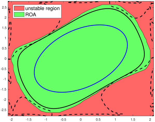
(a) The Van der Pol system

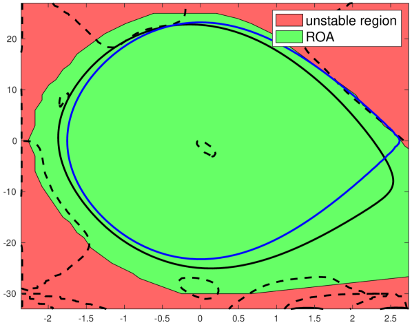
(b) The SMIB system

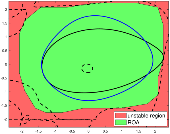
(c) A two machine system

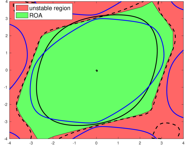
(d) IEEE three machine system

Figure 1: Our estimations of the ROA of several systems, given by the union of the region contained inside the black ($V_{1}$) and blue ($V_{2}$) curves. The dotted line corresponds to the boundary of the $0$-sublevel set of the derivative of $V_{1}$ along the solution map.

VI Numerical Examples

We next present several numerical examples demonstrating how Thm. 3 can be used to yield accurate ROA approximations of nonlinear ODEs. For each numerical example we compute $V_{1}$ and $V_{2}$, from Thm. 3, by respectively fitting Bernstein polynomials to the converse LF given in Eq. (3) (using Eqs. (4), (6) and (7)) and either using an energy function or an analytical LF (found previously in the literature).

To demonstrate the accuracy of our approximations of the ROA we will carry out extensive Monte Carlo simulations of the solution map to estimate the stable and unstable regions in each figure. Although this Monte Carlo method can estimate the ROA well it does not account for simulation error or provide a LF and hence cannot provide a certified ROA inner approximation.

VI-A Estimating the ROA of the Van der Pol system

Consider the reverse time Van der Pol oscillator defined by the vector field:

$$f_{VDP}(x)=\begin{bmatrix}-x_{2}\\ x_{1}-x_{2}(1-x_{1}^{2})\end{bmatrix}$$ (17)

The following quadratic LF was found in [11]: $V_{VDP}(x)=x^{\top}Px$, where $P=\begin{bmatrix}1.5&-0.5\\ -0.5&1\end{bmatrix}$.

We now fit the converse LF, $V^{*}_{\lambda,\beta}$ (given in Eq. (3)), for $\lambda=3$ and $\beta=1$ by a degree $75$ Bernstein polynomial over the set $D=[-2,2]\times[-2.7,2.7]$. In Fig. 1(a) we have plotted our estimation of the ROA achieved using this fitted Bernstein polynomial as $V_{1}$ and $V_{VDP}$ as $V_{2}$ in Thm. 3. The black and blue curves correspond to the boundaries of $\{x\in D:V_{1}(x)<0.74\}$ and $\{x\in D:V_{2}(x)<2.25\}$ respectively.

VI-B Estimating the ROA of the Single Machine Infinite Bus (SMIB) system

The SMIB system can be modeled by an ODE (1) with the following vector field:

$$f_{SMIB}(x):=\begin{bmatrix}x_{2}\\ (1/2H)({P_{m}-\frac{E^{\prime}E_{B}}{X_{eq}}sin(x_{1}+\delta_{ep})-{D}x_{2}})\end{bmatrix},$$

where $H=0.0106s^{2}/rad$, $X_{eq}=0.28pu$, $P_{m}=1pu$, $E_{B}=1pu$, $E^{\prime}=1.21pu$, $D=0.03$. It is shown in [14] that the energy of the SMIB system can be expressed as the following function

$$V_{E}(x):=-P_{m}x_{1}+\frac{E^{\prime}E_{B}}{X_{eq}}(\cos(\delta_{ep})-\cos(x_{1}+\delta_{ep}))+Hx_{2}^{2}.$$

By graphically solving Opt. (13) for $V_{2}=V_{E}$ and $f=f_{SMIB}$, we find $\gamma^{*}_{3}=5.722$. The boundary of $\{x\in\mathbb{R}^{n}:V_{E}(x)\leq\gamma^{*}_{3}\}$ is given as the blue curve in Fig. 1(b)

We find a candidate $V_{1}$ function of Thm. 3 by fitting a degree $60$ Bernstein polynomial to the converse LF, $V^{*}_{\lambda,\beta}$ (given in Eq. (3)), for $\lambda=10$ and $\beta=1$ over the set $D=[-0.75\pi,\pi]\times[-30,30]$.

We have plotted the boundary of $\{y\in D:V_{1}(y)\leq 0.68\}$ as the black curve in Fig. 1(b). These sublevel sets are such that Thm. 3 shows $\{y\in D:V_{1}(y)\leq 0.68\}\cup\{y\in D:V_{2}(y)\leq 5.722\}\subseteq ROA_{f_{SMIB}}$, providing an inner approximation of $ROA_{f_{SMIB}}$. Moreover, we have plotted the boundary of the set $\{y\in D:\nabla V_{1}(y)^{\top}f_{SMIB}(y)\leq 0\}$ as the dotted black line. Showing $\nabla V_{1}(y)^{\top}f_{SMIB}(y)$ may not be negative around a neighborhood of the origin as expected from Sec. V.

Using both $V_{1}$ and $V_{2}$ we have improved the inner approximation of $ROA_{f_{SMIB}}$ as compared to the approximation of yielded by the energy function, $V_{2}$, alone.

VI-C Estimating the ROA of a two-machine versus infinite bus system

Consider the following four dimensional power system model found in [15, 10] that represents a two-machine versus infinite bus system which can be modeled by an ODE (1) with the following vector field:

$$f_{TMIB}(x)=\begin{bmatrix}f_{1}(x),f_{2}(x),f_{3}(x),f_{4}(x)\end{bmatrix}^{\top},$$ (18)

where $f_{1}(x)=x_{2}$, $f_{2}(x)=33.5849-1.8868\cos(x_{1}-x_{3})-5.283\cos(x_{1})-16.9811\sin(x_{1}-x_{3})-59.6226\sin(x_{1})-1.8868x_{2}$, $f_{3}(x)=x_{4}$ and $f_{4}(x)=11.3924\sin(x_{1}-x_{3})-1.2658\cos(x_{1}-x_{3})-3.2278\cos(x_{3})-1.2658x_{4}-99.3671\sin(x_{3})+48.481$. The point $x_{SEP}:=[0.468,0,0.463,0]^{\top}\in\mathbb{R}^{4}$ is a stable equilibrium point of Eq. (18). Using a change of variables $\tilde{x}=x-x_{SEP}$ we map the equilibrium point to the origin.

We now fit the converse LF, $V^{*}_{\lambda,\beta}$ (given in Eq. (3)), for $\lambda=1$ and $\beta=1$ by a degree $20$ Bernstein polynomial over the set $[-2,2]\times[-3,3]\times[-2,2]\times[-3,3]$. Fig. 1(c) shows a slice of the state space when $x_{2}=x_{4}=0$ depicting the sublevel set of this Bernstein polynomial along with the ROA estimation found in [10]. By using Thm. 3 we are able to certify an improved ROA estimation (the union of the sublevel sets in Fig. 1(c)).

VI-D Estimating the ROA of a three-machine system

Consider the following four dimensional power system model found in [16] (Page 144) that represents a three-machine system with machine number 3 as swing bus (reference of the system) and can be modeled by an ODE (1) with the following vector field:

$$f_{3MS}(x)$$ (19)

$$=\begin{bmatrix}x_{2}\\ -\sin(x_{1})-0.5\sin(x_{1}-x_{3})-0.4x_{2}\\ x_{4}\\ -0.5\sin(x_{3})-0.5\sin(x_{3}-x_{1})-0.5x_{4}+0.05\end{bmatrix}$$

The point $x_{SEP}:=[0.02001,0,0.06003,0]^{\top}\in\mathbb{R}^{4}$ is a stable equilibrium point of Eq. (19). Using a change of variables $\tilde{x}=x-x_{SEP}$ we map the equilibrium point to the origin. The ROA of this system has previously been estimated using energy functions in [16]. A more accurate ROA estimation was found in [10] using Sum-of-Squares to find a LF. We now use the LF found in [10] as $V_{2}$ in Thm. 3 and compute a $V_{1}$ by fitting a degree $20$ Bernstein polynomial to the converse LF, $V^{*}_{\lambda,\beta}$ (given in Eq. (3)), for $\lambda=1$ and $\beta=1$ over the set $[-4,4]\times[-0.75,0.75]\times[-4,4]\times[-0.75,0.75]$. Fig. 1(d) shows a slice of the state space when $x_{2}=x_{4}=0$ and depicts the best ROA estimation found in [10] along with a sublevel set of the resulting fitted Bernstein polynomial. Thm. 3 can be used to certify the union of these sublevel sets are inside the ROA, providing an improved ROA estimation.

VII Conclusion

This work proposes a novel methodology for ROA estimation using an approximated converse Lyapunov function, derived from trajectory data, together with an analytical Lyapunov function. The method yields a certifiable inner ROA estimation. Numerical examples demonstrate that the proposed method is able to expand ROA approximations found using analytical Lyapunov functions derived elsewhere in the literature. This method is not limited to the converse Lyapunov function fitting technique implemented, Bernstein polynomial approximations. Function fitting techniques that are better suited for high dimensional problems will be explored in future work.

References

• [1] P. Kundur, N. J. Balu, and M. G. Lauby, Power system stability and control.   McGraw-hill New York, 1994, vol. 7.
• [2] Y.-H. Moon, B.-K. Choi, and T.-H. Roh, “Estimating the domain of attraction for power systems via a group of damping-reflected energy functions,” Automatica, vol. 36, no. 3, pp. 419–425, 2000.
• [3] L. Jin, H. Liu, R. Kumar, J. D. Mc Calley, N. Elia, and V. Ajjarapu, “Power system transient stability design using reachability based stability-region computation,” in Proceedings of the 37th Annual North American Power Symposium, 2005.   IEEE, 2005, pp. 338–343.
• [4] Z. Shuai, C. Shen, X. Liu, Z. Li, and s. John Shen, “Transient angle stability of virtual synchronous generators using lyapunov’s direct method,” IEEE Transactions on Smart Grid, vol. 10, no. 4, pp. 4648–4661, July 2019.
• [5] J. H. Chow, A. Chakrabortty, M. Arcak, B. Bhargava, and A. Salazar, “Synchronized phasor data based energy function analysis of dominant power transfer paths in large power systems,” IEEE Transactions on Power Systems, vol. 22, no. 2, pp. 727–734, May 2007.
• [6] M. Ma, W. Jie, Z. Wang, and M. W. Khan, “Global geometric structure of the transient stability regions of power systems,” IEEE Transactions on Power Systems, pp. 1–1, 2019.
• [7] C. Zhai and H. D. Nguyen, “Estimating the region of attraction for power systems using gaussian process and converse lyapunov function,” IEEE Transactions on Control Systems Technology, 2021.
• [8] B. K. Colbert and M. M. Peet, “Using trajectory measurements to estimate the region of attraction of nonlinear systems,” in 2018 IEEE Conference on Decision and Control (CDC).   IEEE, 2018.
• [9] B. Lai, T. Cunis, and L. Burlion, “Nonlinear trajectory based region of attraction estimation for aircraft dynamics analysis,” in AIAA Scitech 2021 Forum, 2021, p. 0253.
• [10] M. Anghel, F. Milano, and A. Papachristodoulou, “Algorithmic construction of lyapunov functions for power system stability analysis,” IEEE Transactions on Circuits and Systems I: Regular Papers, vol. 60, no. 9, 2013.
• [11] H. K. Khalil, Nonlinear systems.   Prentice hall, 2002.
• [12] M. Jones and M. M. Peet, “Converse lyapunov functions and converging inner approximations to maximal regions of attraction of nonlinear systems,” arXiv preprint arXiv:2103.12825, 2021.
• [13] A. Y. Veretennikov and E. Veretennikova, “On partial derivatives of multivariate bernstein polynomials,” Siberian Advances in Mathematics, vol. 26, no. 4, 2016.
• [14] J. Chow and J. J. Sanchez-Gasca, Power System Modeling, Computation, and Control.   JohnWiley & Sons Ltd, 2020.
• [15] N. Bretas and L. Alberto, “Lyapunov function for power systems with transfer conductances: extension of the invariance principle,” IEEE Transactions on Power Systems, vol. 18, no. 2, p. 769–777, May 2003.
• [16] H.-D. Chiang, Direct methods for stability analysis of electric power systems: theoretical foundation, BCU methodologies, and applications.   John Wiley & Sons, 2011.