Noise Electrometry of Polar and Dielectric Materials

Abstract

A qubit sensor with an electric dipole moment acquires an additional contribution to its depolarization rate when it is placed in the vicinity of a polar or dielectric material as a consequence of electrical noise arising from polarization fluctuations in the material. Here, we characterize this relaxation rate as a function of experimentally tunable parameters such as sample-probe distance, probe-frequency, and temperature, and demonstrate that it offers a window into dielectric properties of insulating materials over a wide range of frequencies and length scales. We discuss the experimental feasibility of our proposal and illustrate its ability to probe a variety of phenomena, ranging from collective polar excitations to phase transitions and disorder-dominated physics in relaxor ferroelectrics. Our proposal paves the way for a novel table-top probe of polar and dielectric materials in a parameter regime complementary to existing tools and techniques.

Polar and dielectric materials exhibit a plethora of interesting correlated physics [1, 2, 3, 4] and are emerging as key components in next-generation solid-state technologies [5, 6, 7, 8, 9]. As a consequence, a multitude of techniques for probing them have been developed, ranging from different forms of microscopy and spectroscopy to electrical transport (Fig. 1b) [10, 11, 12, 13, 14, 15, 16]. While these methods have led to incredible scientific progress, answering several prominent questions such as the origin of polar instabilities in ultra-thin ferroelectric films [9] and the structure of polar domains in relaxor ferroelectrics [17] remains a formidable challenge. In part, this is due to the difficulty of probing the near-equilibrium polar dynamics of thin samples over a wide range of length and time scales simultaneously [9] — which at present requires the use of high-intensity synchrotron light sources. As such, developing a table-top probe with the requisite frequency and spatial resolution would naturally complement existing experimental probes of polar and dielectric materials.

The advent of nanoscale quantum sensors, typically based upon impurities embedded in insulating materials, provides an avenue for developing such a probe. Such sensors are often excellent AC electrometers and magnetometers; they can probe a wide range of frequencies and can locally image both static configurations and dynamic fluctuations of electromagnetic fields with nanoscale resolution [18, 19, 20, 21, 22, 23]. Indeed, a number of theoretical proposals and pioneering experiments have utilized their magnetic field sensing capabilities to probe spin dynamics and electrical current fluctuations in solid-state systems [24, 25, 26, 27, 28, 29, 30, 31, 32, 33, 34, 35, 36, 37, 38, 39, 40, 41, 42, 43, 44, 45, 46, 47, 21, 48].

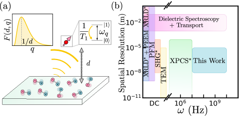
Figure 1: (a) Schematic of qubit sensing experiment. A probe qubit (top right), with splitting $\omega_{q}$, is a distance $d$ away from a polar or dielectric material. Fluctuations in the material’s dipoles lead to electrical noise at the location of qubit causing the qubit to relax from $\ket{1}$ to $\ket{0}$ at a rate $1/T_{1}$. The qubit is sensitive to fluctuations at frequency $\omega_{q}$ and wavevectors around $1/d$ (see filter on top left). (b) Regimes of applicability of qubit sensors and other probes including microscopy techniques [atomic-force, piezoresponse-force, and transmission electron microscopy (AFM, PFM, and TEM)], spectroscopy techniques [x-ray photon correlation, x-ray linear dichroism, and second harmonic generation spectroscopy (XPCS, XRLD, and SHG)] and electrical transport techniques [10, 11, 12, 13, 14, 15, 16, 49]. Techniques that often require high intensity light sources are marked with a $*$.

In this Letter, we show that the electrical sensing capabilities of single-qubit sensors can be used to probe the near-equilibrium physics of polar and dielectric materials, even in the thin-film context. In particular, we demonstrate that the relaxation rate of a qubit in the presence of electrical noise arising from such materials encodes the material’s dielectric properties at frequencies set by the energy splitting of the qubit and wave vectors set by the qubit-sample distance. Hence, by tuning these two parameters, such qubit sensors can non-invasively and wirelessly probe polar and dielectric materials on frequency scales between $10$ $\text{ MHz}-10\leavevmode\nobreak\ \text{GHz}$ down to nanometer length scales and over a wide range of temperatures, $1$ K - $600$ K [50, 51, 52]. To highlight the utility of these sensors, we demonstrate how they can (i) detect the presence of exotic collective excitations in polar fluids, (ii) characterize paraelectric-to-ferroelectric phase transitions that underlie polar instabilities, and (iii) probe local polar dynamics in relaxor ferroelectrics. Finally, we illustrate the feasibility of qubit sensing via concrete numerical estimates for the relaxation rate of a nitrogen-vacancy (NV) center in diamond placed near a polar material (strontium titanate).

Qubit Relaxometry Concept—Our experimental proposal is depicted schematically in Fig. 1a wherein we envision an isolated impurity qubit sensor placed a distance $d$ away from a polar or dielectric material. This qubit is a two-level system with a ground state $\ket{0}$ split in energy from an excited state $\ket{1}$ by $\hbar\omega_{q}$ and its quantum state can be initialized, measured, and manipulated optically. Moreover, we consider qubits with an electric dipole moment $\hat{\mathbf{d}}=d_{\perp}(\sigma_{x}\hat{x}+\sigma_{y}\hat{y})$ and a magnetic moment $\hat{\boldsymbol{\mu}}=\mu_{z}\sigma_{z}\hat{z}$, where $\boldsymbol{\sigma}$ are the Pauli matrices, which specifies their coupling to electromagnetic fields as $H_{\text{q-EM}}=\hat{\mathbf{d}}\cdot\mathbf{E}+\hat{\boldsymbol{\mu}}\cdot\mathbf{B}$. As a result, electric fields $\mathbf{E}$ drive transitions between $\ket{0}$ and $\ket{1}$ and magnetic fields $\mathbf{B}$ can be utilized to control their frequency splitting. When placed close to a polar or dielectric material, electrical noise emanating from the material will couple the two states of the qubit and cause the qubit, initialized in its excited state, to naturally relax to a thermal equilibrium set by the ambient temperature, $T$. The rate of this relaxation can be expressed in terms of a time-scale $T_{1}$ and can be computed from Fermi’s Golden Rule as:

$$\frac{1}{T_{1}}=\frac{d_{\perp}^{2}}{2}\coth\left(\frac{\beta\omega_{q}}{2}\right)\int_{-\infty}^{\infty}dt\ \langle[E_{-}(t),E_{+}(0)]\rangle e^{i\omega_{q}t}\leavevmode\nobreak\ \leavevmode\nobreak\ \leavevmode\nobreak\ \leavevmode\nobreak\$$ (1)

where the electrical noise is quantified via the auto-correlation function $\langle[E_{-}(t),E_{+}(0)]\rangle$ with $E_{\pm}=E_{x}\pm iE_{y}$, $\beta=1/k_{B}T$, and $\langle\cdots\rangle$ denotes thermal averaging. Intuitively, Eq. (1) expresses that only electrical noise at a frequency resonant with the splitting of the qubit contributes to its relaxation rate.

To understand how the relaxation rate is connected to the dielectric properties of the underlying material, we note that the electrical noise responsible arises from thermal or quantum fluctuations of the material’s polarization density $\mathbf{P}$. The fluctuations at frequency $\omega$ and wavevector ${\mathbf{q}}$ can be quantified by the retarded polarization correlation function $\chi_{\alpha\beta}(\omega,{\mathbf{q}})=i\int_{0}^{\infty}dt\,e^{i\omega t}\langle[P_{\alpha}^{\dagger}(t,{\mathbf{q}}),P_{\beta}(0,{\mathbf{q}})]\rangle$ ($\alpha,\beta=x,y,z$) which determines the dielectric tensor of the material, $\varepsilon_{\alpha\beta}(\omega,{\mathbf{q}})$, and thus encodes its electrical response  [53, 54, 55]. By utilizing these correlation functions, we can formalize the relationship between fluctuations of polarization in the material and electrical noise at the qubit. For simplicity, we assume that the material is a stack of $N$, weakly inter-correlated, two-dimensional (2D) monolayers spaced apart by a distance $w$ (modeling a thin-film) and is both translationally and rotationally invariant (see supplementary material for generalizations) [56]. From Maxwell’s equations, polarization fluctuations of this sample propagate to electrical noise as:

$$\langle[E_{-}(t),E_{+}(0)]\rangle=\mu_{0}^{2}\int\frac{d\omega\ d^{2}{\mathbf{q}}}{(2\pi)^{3}}\ F(d,q)\mathcal{C}(\omega,{\mathbf{q}})e^{-i\omega t}\leavevmode\nobreak\ \leavevmode\nobreak\ \leavevmode\nobreak\$$ (2)

where $\mathcal{C}(\omega,{\mathbf{q}})=\text{Im}\left[\chi_{+-}(\omega,{\mathbf{q}})+\chi_{-+}(\omega,{\mathbf{q}})+4\chi_{zz}(\omega,{\mathbf{q}})\right]$, and $F(d,q)=\sum_{j=0}^{N-1}q^{2}e^{-2q(d+jw)}/16$ filters polarization fluctuations at different wavevectors. Crucially, $F(d,q)$ is sharply peaked at $1/d$ and so the qubit will only see fluctuations in the polarization around this wavevector. By combining Eqs. (1) and (2), we find that:

$$\frac{1}{T_{1}}=\frac{d_{\perp}^{2}\mu_{0}^{2}}{2}\coth\left(\frac{\beta\omega_{q}}{2}\right)\int\frac{d^{2}{\mathbf{q}}}{(2\pi)^{2}}F(d,q)\mathcal{C}(\omega_{q},{\mathbf{q}})\leavevmode\nobreak\ \leavevmode\nobreak\ \leavevmode\nobreak\ \leavevmode\nobreak\$$ (3)

Therefore, by tuning the frequency splitting of the qubit $\omega_{q}$ and the qubit-sample distance $d$, one can effectively reconstruct the functional form of $\mathcal{C}(\omega,{\mathbf{q}})$ [57]. Thus, measuring the qubit’s relaxation rate gives one access to the dielectric properties of a proximate material.

A few remarks are in order. First, we note that existing qubit sensing setups have demonstrated the capability to tune a probe qubit’s frequency between $10\ \text{MHz}-10\ \text{GHz}$, have reached qubit-sample distances down to $\sim 10$ nm, and have operated between $1-600\leavevmode\nobreak\ \text{K}$ [58, 59, 60]. The parameter regimes accessible by qubit sensors and other equilibrium/near-equilibrium probes of polar and dielectric materials are depicted in Fig. 1b [56, 10, 11, 12, 13, 14, 15, 16, 49] which highlights that our probe can nicely complement existing experimental techniques. Second, we note that the frequency scales accessible to qubit sensors are small relative to the excitation energy scales of typical materials. As a result, they will be sensitive to gapless or weakly gapped polar excitations.

Applications—The ability to probe such excitations naturally enables qubit sensors to address questions about polar and dielectric materials relevant to both fundamental and applied science. We examine in detail three such questions.

To begin, we discuss how the qubit sensor can detect collective modes in neutral polar fluids. While the existence of “plasmon” collective modes, arising from long-range Coulomb interactions between charged electrons in metals, has been well established [61], the conclusive observation of their dipolar analogues—“dipolarons”—has remained an outstanding challenge [62, 63, 64]. Dipolarons in a 2D dipolar fluid with density $n_{d}$, molecular mass $m$, and dipole moment $\boldsymbol{\mu}$ are predicted to be gapless [56, 62] with an unusual dispersion $\omega_{d}^{2}({\mathbf{q}})=v^{2}q^{2}+2\pi n_{d}q({\mathbf{q}}\cdot\boldsymbol{\mu})^{2}/m$, which is anisotropic due to the directional dependence of the dipolar interaction. Dispersion in hand, we can predict the frequency and distance scaling of the relaxation rate $1/T_{1}$ of a nearby qubit. In particular, for a general polar mode with dispersion $\omega({\mathbf{q}})$ and gap $\omega_{0}$, the polarization correlations take the form $\chi_{-+}(\omega,{\mathbf{q}})\sim(\omega-\omega({\mathbf{q}})+i0^{+})^{-1}$ and hence $1/T_{1}$ is given by [56, 65]:

$$\frac{1}{T_{1}}\sim\coth\left(\frac{\beta\omega_{q}}{2}\right)\times\left[e^{-2q_{res}d}q_{res}^{2}\right]\Theta(\omega_{q}-\omega_{0})$$ (4)

where $q_{\text{res}}$ satisfies $\omega(q_{\text{res}})=\omega_{q}$. Thus, for gapless dipolarons in particular, the crossover from a linear to $q^{3/2}$ dispersion with increasing $q$ manifests in a corresponding crossover in the frequency scaling of $1/T_{1}$ from $\omega_{q}e^{-2\omega_{q}d/v}$ to $\sim\omega_{q}^{1/3}e^{-2(\omega_{q})^{2/3}d}$, and can serve as a smoking gun signature of these collective modes.

The ability to probe low-energy polar excitations further enables qubit sensors to characterize phase transitions in polar and dielectric materials. While such transitions are well-understood in three dimensions (3D), their nature is unclear in 2D; coupling to additional low-energy modes, irrelevant in 3D, could dramatically alter the universal properties of the transition [66]. Furthermore, previous experiments aimed at fabricating thin-film ferroelectrics for device applications have encountered instabilities in the material’s polarization, suspected to be intimately related to the stability of the 2D paraelectric to ferroelectric (PE/FE) phase transition [67]. Motivated by these outstanding questions, we make predictions for the behavior of $1/T_{1}$ across a continuous PE/FE phase transition.

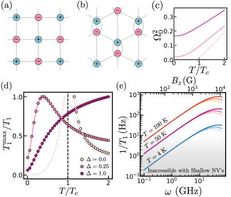
Figure 2: (a, b) Schematic of ionic crystal in the (a) PE phase and the (b) FE phase. (c, d) Behavior of $1/T_{1}$ across a relaxor ferroelectric for disorder $\Delta=0.0,0.25,1.0$ (see Panel (d) for legend). The presence of disorder causes a polarization-carrying mode to open a gap which can drastically change the response of qubit sensors. (e) Numerical estimate for $1/T_{1}^{\text{sig}}$ compared to intrinsic relaxation rate of the NV qubit as a function of frequency, $\omega$, and applied magnetic field, $B_{z}$. $1/T_{1}$ is depicted for temperatures $T=4\ \text{K},50\ \text{K},100\ \text{K}$ (shown in blue, purple, and red respectively) and distances $d=30,50,70\text{ nm}$ (depicted as shading from dark to light). For all parameters shown, the relaxation rate is above experimental limits of $1/T_{1}$ determined in Ref. [68].

The PE/FE transition is a structural phase transition accompanied by inversion-symmetry breaking and a spontaneously generated polarization density. It can be visualized by considering an ionic crystal with alternating charges $\pm Q$ shown in both the PE and FE phase in Fig. 2(a, b) respectively. This transition is driven by the softening of transverse optical phonon modes which correspond to the relative displacement between the $\pm Q$ charges depicted. The mechanism underlying this softening is either thermal or quantum fluctuations depending on whether the transition is driven by temperature (a “thermal phase transition”) or a separate tuning parameter $\lambda$ (e.g. strain) at $T=0$ (a “quantum phase transition”) [61, 69]. If we assume that these phonon modes do not interact and have dispersion $\omega^{2}({\mathbf{q}})=c_{s}^{2}{\mathbf{q}}^{2}+\omega_{0}^{2}$ with $\omega_{0}\to 0$ at the transition, from Eq. (4) we find that once $\omega_{0}$ is less than the frequency splitting of the qubit, the qubit sensor will detect its presence. Although interactions will dramatically affect the polarization correlations near the transition and hence the scaling of $1/T_{1}$, this simple analysis illustrates that qubit sensors are ideal for probing the critical physics around the transition. This motivates a more careful analysis of $1/T_{1}$ around a critical point by using dynamical scaling theories for both thermal and quantum transitions [61].

Around the critical point $\lambda=\lambda_{c}$, the static correlations of the polarization are set by a diverging correlation length $\xi\propto|\lambda-\lambda_{c}|^{-\nu}$, while dynamics are strongly constrained by symmetries. Since the polarization density is not conserved, the corresponding dynamics are relaxational, characterized by a order-parameter relaxation rate $\Gamma$. A key difference between thermal and quantum phase transitions is how they behave upon changing $T$ in the vicinity of the critical point. Thermal transitions are driven by $T$ and hence both $\xi$ and $\Gamma$ scale as a power law of the distance from the critical point $t=(T-T_{c})/T_{c}$. Consequently, we can conclude using the dynamic scaling theory of critical phenomena [56, 70, 71, 72, 73] that:

$$\frac{1}{T_{1}}\sim\frac{2T}{d^{2+\eta-z}}\Psi_{t}\left(\omega d^{z},\frac{\xi}{d}\right),\leavevmode\nobreak\ \leavevmode\nobreak\ \xi\propto|t|^{-\nu}$$ (5)

where $\Psi_{t}$ is a scaling function, $\eta$, $\nu$, and $z$ are critical exponents. If $\Psi_{t}$ is smooth in the $\omega\rightarrow 0$ limit, then $1/T_{1}$ scales with qubit-sample distance as $d^{-2-\eta+z}$ at the critical point in stark contrast to the non-critical regime where it scales as $1/d^{4}$; a change in the distance dependence of $T_{1}$ is a tell-tale signature of approaching thermal criticality. In addition, a scaling analysis near $T_{c}$ enables extracting critical exponents $\eta$, $z$ and $\nu$. On the other hand, if we tune to a quantum critical point ($\lambda=\lambda_{c}$) and raise $T$ from $0\text{ K}$, then the lack of any gap scale in the spectrum ($\omega_{0}=0$) implies that both the correlation length $\xi\sim c_{s}/T^{1/z}$ and relaxation rate $\Gamma\sim T$ are solely determined by temperature. This can be used to show that $1/T_{1}$ scales as a power law in $T$ (rather than $T-T_{c}$), with a distinct distance dependence [56, 74, 61]:

$$\frac{1}{T_{1}}\propto\begin{cases}T^{(2+\eta)/z}\log\left(\dfrac{c_{s}}{dT^{1/z}}\right),\leavevmode\nobreak\ d\ll\xi\\[8.0pt] T^{(-2+\eta)/z}{d^{-4}},\leavevmode\nobreak\ d\gg\xi.\end{cases}$$ (6)

While the distance-scaling of $1/T_{1}$ informs us of whether we are in the critical regime, its temperature-scaling can be used to determine the critical exponents $\eta$ and $z$. Finally, the dependence of the spectral gap $\omega_{0}\propto|\lambda-\lambda_{c}|^{\nu z}$ on the tuning parameter $\lambda$, derived from low-T activated behavior of $1/T_{1}$, may be used to deduce the critical exponent, $\nu$. Thus, all critical exponents for the quantum transition may be deduced by an analysis of the qubit’s relaxation rate as a function of $T$, $d$ and $\lambda-\lambda_{c}$.

Up until this point, we have explored clean systems without quenched disorder. However, it is known that disorder can dramatically affect the behavior of low-dimensional materials [75]. A prototypical example is in relaxor ferroelectrics (relaxors), dielectric materials characterized by anomalously large internal polar fluctuations resembling “disorder broadened” critical correlations of phase transitions [76, 77, 78, 79, 80]. While a full microscopic description of relaxors is missing, their properties are often attributed to competition between the long-range dipolar interaction, which orders internal dipoles, and short-range disorder, which freezes them in a particular direction [81, 82, 80]. This competition is captured by a minimal classical model of dipoles arranged in a 2D lattice [82, 83]:

$$H=\sum_{i}\left[\frac{\Pi_{i}^{2}}{2M}+V(u_{i})-h_{i}u_{i}\right]-\sum_{i<j}v_{ij}u_{i}u_{j}\leavevmode\nobreak\ \leavevmode\nobreak\ \leavevmode\nobreak\$$ (7)

where $\Pi_{i}=M\dot{u}_{i}$ is the conjugate momentum of the polarization-carrying displacement $u_{i}$ chosen to be along the $z$-axis, $M$ is the effective mass, $v_{ij}$ is the dipolar interaction, $h_{i}$ is a normally distributed random field with width $\Delta$, and $V(u_{i})=\frac{\kappa}{2}u_{i}^{2}+\frac{\gamma}{4}u_{i}^{4}$ ($\kappa,\gamma>0$) is an anharmonic potential. When our impurity qubit is far from the material ($d\gg\sqrt{A}$ where $A$ is the area of a polar region), the qubit is insensitive to the local realization of $h_{i}$ and encodes the disorder-averaged dynamics of the relaxor. Here, the polarization correlations take a damped harmonic form $\chi_{zz}(\omega,{\mathbf{q}})=(M\Omega^{2}({\mathbf{q}})-M\omega^{2}+i\omega\Gamma)^{-1}$ where $\Omega^{2}({\mathbf{q}})=\Omega_{0}^{2}+(v_{0}-v_{\mathbf{q}})$, $v_{\mathbf{q}}$ is the Fourier transformed dipolar interaction, $v_{0}=\lim_{{\mathbf{q}}\to 0}v_{\mathbf{q}}$, $\Gamma$ is a phenomenological damping, and $\Omega_{0}$ is determined self-consistently in a mean-field analysis and is depicted in Fig. 2(c) in the clean, weak disorder, and strong disorder case ($\Delta=0,0.25,1.0$, respectively) [56, 81, 82, 80, 84, 85]. From the mode frequency $\Omega_{0}^{2}$ at $\Delta=0$, we can extract a critical temperature $T_{c}$ defined as the temperature where the mode becomes massless. Mode frequency and critical temperature in hand, we numerically compute $1/T_{1}$ in a temperature range around $T=T_{c}$ and normalize $1/T_{1}$ by its maximum in that range, $1/T_{1}^{\text{max}}$ (Fig. 2(d)). We find that, in the clean case $\Delta=0$, the relaxation rate becomes sharply peaked at the location of the phase transition, whereas for weak disorder ($\Delta=0.25$) the response broadens, reproducing our earlier intuition. For sufficiently large disorder, the peak is removed entirely and the relaxation rate increases monotonically on lowering $T$.

On the other hand, when our impurity qubit is sufficiently close to the material ($d\sim\sqrt{A}$), the qubit will be able to resolve the microscopic dynamics of individual polar domains and the assumption of translation invariance of Eq. 3 will no longer hold. Here we present a qualitative picture of the physics made accessible by spatio-temporally resolving these polar dynamics. Relaxor ferroelectrics are often modeled using polar nano-regions — static nanoscale polar domains with non-zero spontaneous polarization pinned by disorder [86, 87, 88]. The presence of such polar nano-regions with quenched fluctuations would imply a suppressed $1/T_{1}$ once the qubit is positioned of top of such a region, and enhanced $1/T_{1}$ when the qubit lies close to a domain wall. On the other hand, recent works have suggested a ‘slush-water’ picture of relaxors [17] characterized by coexisting static (ice-like) domains with frozen moments and dynamic (water-like) domains with fluctuating polarization; above an ice-like domain, $1/T_{1}$ would be suppressed, while above a water-like domain, $1/T_{1}$ would be an enhanced. By studying $1/T_{1}$ of an isolated qubit as a function of in-plane coordinates at a fixed distance $d\lesssim\sqrt{A}$, a spatially resolved map of the static and dynamic domains in an inhomogeneous sample could be obtained and aid in evincing a microscopic description of relaxors.

Experimental Realization and Feasibility—While our previous discussion has theoretically motivated the utility of qubit sensing in probing polar and dielectric materials, here we discuss a concrete realization of the qubit sensing setup and its feasibility. In particular, we envision utilizing the NV center in diamond: a point defect consisting of a nitrogen substitution adjacent to a lattice vacancy defect. The ${}^{3}A_{2}$ electronic spin manifold of the NV is modeled as a three-level system ($\ket{0},\ket{+},$ and $\ket{-}$) and the degenerate $\ket{\pm}$ states are ideal for encoding the two-level qubit of our proposal [89]. Crucially, these degenerate states can be initialized and manipulated optically and read-out through state-dependent fluorescence [90]. Moreover, as required, electric fields drive transitions between these states with dipole moment $d_{\perp}=17\ \mathrm{Hz}\cdot\mathrm{cm/V}$ and magnetic fields control their splitting with a magnetic moment of $\mu_{z}=2.8\text{ MHz}/\text{G}$ [91, 90]. As a result, the splitting of the NV can be controlled by local magnetic fields and the qubit-sample distance can be controlled by, for example, placing a nano-diamond with a single NV on a scanning probe tip [32, 28, 35, 24], enabling a measurement of $1/T_{1}$ as a function of both frequency and distance.

To assess the feasibility of this proposal, we express the relaxation rate of the NV as $T_{1}^{-1}=(T_{1}^{\textrm{sig}})^{-1}+(T_{1}^{\textrm{int}})^{-1}$, where $(T_{1}^{\textrm{sig}})^{-1}$ accounts for the signal from the sample and $(T_{1}^{\textrm{int}})^{-1}$ accounts for intrinsic sources of relaxation from the diamond host, whose magnitude establishes a limit on the sensitivity of our sensing protocol. The magnitude of $(T_{1}^{\textrm{int}})^{-1}$ has been reported in shallow NV samples ($\sim 50\leavevmode\nobreak\ \textrm{nm}$ depth) as low as $10\leavevmode\nobreak\ \textrm{Hz}$ below $100\leavevmode\nobreak\ \textrm{K}$ [68, 92]. The feasibility of our proposal can be established by comparing this noise floor to the expected signal magnitude in a paradigmatic setting: the ionic crystal model introduced earlier with a density $\rho$, lattice spacing $a$ (See Fig. 2(a,b)), and polarization-carrying phonon mode with dispersion $\omega_{d}({\mathbf{q}})=\sqrt{c_{s}^{2}q^{2}+\omega_{0}^{2}}$ with $c_{s}$ equal to the mode speed. In this case, $(T_{1}^{\text{sig}})^{-1}$ takes the form of Eq. 4 with a dimensionful multiplier $\mathcal{N}=(\pi/2c_{s}^{2})\times(\mu_{0}^{2}d_{\perp}^{2}c^{4}/64\pi)\times\left[(Q^{2}/a^{4})\times(\hbar/\rho)\right]$ [56]. Choosing material parameters $\{a,\rho,c_{s},\omega_{0},Q,w,N\}=$ $\{0.3905\text{ nm},183\text{ amu}/a^{2},7.5\cdot 10^{3}\text{ m}/\text{s},0\text{ GHz},9.66\text{ e},a,300$ $\text{ layers}\}$, motivated from a representative dielectric material (thin-film strontium titanate) [93, 94, 95], we can now compare $(T_{1}^{\textrm{sig}})^{-1}$ as a function of frequency, distance, and temperature, to our noise floor, $(T_{1}^{\textrm{int}})^{-1}$ as depicted in Fig. 2(e). For the parameters chosen, the signal magnitude is found to be significantly larger than currently accessible NV intrinsic relaxation rates over a wide range of temperatures and frequencies.

We note that in our feasibility analysis, we assumed that excitations above the ground state are non-interacting and long-lived. While this assumption only holds in the limit of dilute excitations, we expect that the presence of interactions will enhance polarization fluctuations. Hence, our estimate is expected to be a lower bound on the relaxation rate and motivates the feasibility of our method generally. We also remark that we have neglected the contribution of magnetic noise, which induces decay from the NV’s $\ket{\pm 1}$ states to $\ket{0}$. While this is appropriate when probing insulating materials because the relaxation rate due to magnetic noise generated from electrical dipoles is smaller than the electrical noise by a factor of $\mu_{z}^{2}c_{s}^{2}/d_{\perp}^{2}c^{4}\sim 10^{-4}\ll 1$ [56], it is not in general true for metals, where the relaxation rate will be dominated by current fluctuations of itinerant electrons.

Conclusions— In this work, we demonstrated that qubit sensors are a promising table-top tool for studying near-equilibrium dynamics in polar and dielectric materials and can probe even thin-film samples over a wide range of frequencies ($\sim 10\text{ MHz}-10\text{ GHz}$) and temperatures ($1-600\ \text{K}$) down to the nanometer scale. These capabilities make such sensors sensitive to low energy polar modes, enabling them to probe a variety of physical phenomena, ranging from collective polarization modes in long-range interacting systems, to paraelectric-to-ferroelectric phase transitions and disorder-induced phenomena in relaxor ferroelectrics. Complementary to existing techniques, the nanoscale spatial resolution of qubit sensors allows us to probe local dynamics in inhomogeneous materials. We briefly comment on a few open directions involving qubit electrometry. First, since previous work has demonstrated the sensing capabilities of impurity qubits at high pressures ($\sim\mathcal{O}(10)\leavevmode\nobreak\ \text{GPa}$), such qubits could naturally investigate the influence of pressure and strain fields on the dynamics of polarization and could aid in characterizing strain-induced phase transitions [96, 97, 98]. In addition, as illustrated in Eq. (3), our qubit probe is more sensitive to surface physics at short sample-probe distances [56]. Consequently, it can be used to resolve surface polarization dynamics, which can be distinct from the bulk [99]. The nanoscale resolution of the qubit is ideally suited to probe unconventional ferroelectricity in moiré materials, which typically have superlattice lengthscales of tens of nanometers [100, 101]. Finally, by using the electrical capabilities of qubit sensors, highlighted in this work, with the previously established magnetic capabilities, one may be able to probe the complex interplay between charge, polarization, and magnetization found in multiferroic materials [1].

Acknowledgments— We gratefully acknowledge discussions with Eugene Demler, Marcin Kalinowski, Francisco Machado, Thomas Mittiga, Joaquin Rodriguez-Nieva, Eric Peterson, Lokeshwar Prasad, and Chong Zu. We would especially like to thank Eugene Demler, Francisco Machado, and Joaquin Rodriguez-Nieva for collaborations on related projects. R.S. acknowledges support from the Barry M. Goldwater Scholarship, UC Berkeley’s Summer Undergraduate Research Fellowship , and by the U.S. Department of Energy, Office of Science, Office of Advanced Scientific Computing Research, Department of Energy Computational Science Graduate Fellowship under Award Number DESC0022158. S.C. was supported by the ARO through the Anyon Bridge MURI program (grant number W911NF-17-1-0323) and the U.S. DOE, Office of Science, Office of Advanced Scientific Computing Research, under the Accelerated Research in Quantum Computing (ARQC) program. E. P. acknowledges support from Intel Corporation under the FEINMAN Program. N.Y.Y. acknowledges support from the U.S. Department of Energy, Office of Basic Energy Sciences, Materials Sciences and Engineering Division, under Contract No. DE-AC02-05-CH11231 within the High Coherence Multilayer Superconducting Structures for Large Scale Qubit Integration and Photonic Transduction Program (QISLBNL).

References

- Das et al. [2019] S. Das, Y. Tang, Z. Hong, M. Gonçalves, M. McCarter, C. Klewe, K. Nguyen, F. Gómez-Ortiz, P. Shafer, E. Arenholz, et al., Nature 568, 368 (2019).
- Kozii et al. [2019] V. Kozii, Z. Bi, and J. Ruhman, Phys. Rev. X 9, 031046 (2019).
- Volkov et al. [2021] P. A. Volkov, P. Chandra, and P. Coleman, “Superconductivity from energy fluctuations in dilute quantum critical polar metals,” (2021), arXiv:2106.11295 [cond-mat.supr-con] .
- Dunnett et al. [2019] K. Dunnett, J.-X. Zhu, N. A. Spaldin, V. Juričić, and A. V. Balatsky, Phys. Rev. Lett. 122, 057208 (2019).
- [5] L. Tu, X. Wang, J. Wang, X. Meng, and J. Chu, Advanced Electronic Materials 4, 1800231.
- Ishiwara [2012] H. Ishiwara, J Nanosci Nanotechnol 12, 7619 (2012).
- Manipatruni et al. [2019] S. Manipatruni, D. E. Nikonov, C.-C. Lin, T. A. Gosavi, H. Liu, B. Prasad, Y.-L. Huang, E. Bonturim, R. Ramesh, and I. A. Young, Nature 565, 35 (2019).
- Chang et al. [2017] S.-C. Chang, A. Naeemi, D. E. Nikonov, and A. Gruverman, Phys. Rev. Applied 7, 024005 (2017).
- Martin and Rappe [2016] L. W. Martin and A. M. Rappe, Nature Reviews Materials , 16087 (2016).
- McCullian et al. [2020a] B. A. McCullian, A. M. Thabt, B. A. Gray, A. L. Melendez, M. S. Wolf, V. L. Safonov, D. V. Pelekhov, V. P. Bhallamudi, M. R. Page, and P. C. Hammel, Nature Communications 11, 5229 (2020a).
- Polisetty et al. [2012] S. Polisetty, J. Zhou, J. Karthik, A. R. Damodaran, D. Chen, A. Scholl, L. W. Martin, and M. Holcomb, Journal of Physics: Condensed Matter 24, 245902 (2012).
- Gruverman et al. [2019] A. Gruverman, M. Alexe, and D. Meier, Nature Communications 10, 1661 (2019).
- Grübel et al. [2008] G. Grübel, A. Madsen, and A. Robert, in Soft Matter Characterization (Springer Netherlands, 2008) pp. 953–995.
- Winkler et al. [2012] C. R. Winkler, M. L. Jablonski, A. R. Damodaran, K. Jambunathan, L. W. Martin, and M. L. Taheri, Journal of Applied Physics 112, 052013 (2012).
- Grigas [2019] J. Grigas, Microwave Dielectric Spectroscopy of Ferroelectrics and Related Materials (CRC Press, 2019).
- Parsonnet et al. [2020] E. Parsonnet, Y.-L. Huang, T. Gosavi, A. Qualls, D. Nikonov, C.-C. Lin, I. Young, J. Bokor, L. W. Martin, and R. Ramesh, Phys. Rev. Lett. 125, 067601 (2020).
- Takenaka et al. [2017] H. Takenaka, I. Grinberg, S. Liu, and A. M. Rappe, Nature 546, 391 (2017).
- Degen et al. [2017] C. L. Degen, F. Reinhard, and P. Cappellaro, Reviews of Modern Physics 89, 035002 (2017), arXiv:1611.02427 [quant-ph] .
- Grinolds et al. [2013] M. S. Grinolds, S. Hong, P. Maletinsky, L. Luan, M. D. Lukin, R. L. Walsworth, and A. Yacoby, Nat Phys 9, 215 (2013).
- Dovzhenko et al. [2018] Y. Dovzhenko, F. Casola, S. Schlotter, T. Zhou, F. Büttner, R. Walsworth, G. Beach, and A. Yacoby, Nature communications 9, 2712 (2018).
- Hsieh et al. [2019] S. Hsieh, P. Bhattacharyya, C. Zu, T. Mittiga, T. Smart, F. Machado, B. Kobrin, T. Höhn, N. Rui, M. Kamrani, et al., Science 366, 1349 (2019).
- Block et al. [2020] M. Block, B. Kobrin, A. Jarmola, S. Hsieh, C. Zu, N. L. Figueroa, V. M. Acosta, J. Minguzzi, J. R. Maze, D. Budker, and N. Y. Yao, “Optically enhanced electric field sensing using nitrogen-vacancy ensembles,” (2020), arXiv:2004.02886 [quant-ph] .
- Mittiga et al. [2018] T. Mittiga, S. Hsieh, C. Zu, B. Kobrin, F. Machado, P. Bhattacharyya, N. Rui, A. Jarmola, S. Choi, D. Budker, and et al., Physical Review Letters 121 (2018).
- Kolkowitz et al. [2015] S. Kolkowitz, A. Safira, A. High, R. Devlin, S. Choi, Q. Unterreithmeier, D. Patterson, A. Zibrov, V. Manucharyan, H. Park, et al., Science 347, 1129 (2015).
- Casola et al. [2018] F. Casola, T. van der Sar, and A. Yacoby, Nature Reviews Materials 3, 17088 (2018), arXiv:1804.08742 [cond-mat.str-el] .
- Agarwal et al. [2017] K. Agarwal, R. Schmidt, B. Halperin, V. Oganesyan, G. Zaránd, M. D. Lukin, and E. Demler, Phys. Rev. B 95, 155107 (2017).
- Rodriguez-Nieva et al. [2018] J. F. Rodriguez-Nieva, K. Agarwal, T. Giamarchi, B. I. Halperin, M. D. Lukin, and E. Demler, Phys. Rev. B 98, 195433 (2018).
- Finco et al. [2021] A. Finco, A. Haykal, R. Tanos, F. Fabre, S. Chouaieb, W. Akhtar, I. Robert-Philip, W. Legrand, F. Ajejas, K. Bouzehouane, N. Reyren, T. Devolder, J.-P. Adam, J.-V. Kim, V. Cros, and V. Jacques, Nature Communications 12, 767 (2021).
- Schäfer-Nolte et al. [2014] E. Schäfer-Nolte, L. Schlipf, M. Ternes, F. Reinhard, K. Kern, and J. Wrachtrup, Phys. Rev. Lett. 113, 217204 (2014).
- Li et al. [2019] C. Li, M. Chen, D. Lyzwa, and P. Cappellaro, Nano Letters 19, 7342 (2019), pMID: 31549847, https://doi.org/10.1021/acs.nanolett.9b02960 .
- Schmid-Lorch et al. [2015] D. Schmid-Lorch, T. Häberle, F. Reinhard, A. Zappe, M. Slota, L. Bogani, A. Finkler, and J. Wrachtrup, Nano Letters 15, 4942 (2015), pMID: 26218205, https://doi.org/10.1021/acs.nanolett.5b00679 .
- Ariyaratne et al. [2018] A. Ariyaratne, D. Bluvstein, B. A. Myers, and A. C. B. Jayich, Nature Communications 9, 2406 (2018).
- Steinert et al. [2013] S. Steinert, F. Ziem, L. T. Hall, A. Zappe, M. Schweikert, N. Götz, A. Aird, G. Balasubramanian, L. Hollenberg, and J. Wrachtrup, Nature Communications 4, 1607 (2013).
- Ermakova et al. [2013] A. Ermakova, G. Pramanik, J.-M. Cai, G. Algara-Siller, U. Kaiser, T. Weil, Y.-K. Tzeng, H. C. Chang, L. P. McGuinness, M. B. Plenio, B. Naydenov, and F. Jelezko, Nano Letters 13, 3305 (2013), pMID: 23738579, https://doi.org/10.1021/nl4015233 .
- Zhou et al. [2021] T. X. Zhou, J. J. Carmiggelt, L. M. Gächter, I. Esterlis, D. Sels, R. J. Stöhr, C. Du, D. Fernandez, J. F. Rodriguez-Nieva, F. Büttner, E. Demler, and A. Yacoby, Proceedings of the National Academy of Sciences 118 (2021), 10.1073/pnas.2019473118.
- McCullian et al. [2020b] B. A. McCullian, A. M. Thabt, B. A. Gray, A. L. Melendez, M. S. Wolf, V. L. Safonov, D. V. Pelekhov, V. P. Bhallamudi, M. R. Page, and P. C. Hammel, Nature Communications 11, 5229 (2020b).
- Rodriguez-Nieva et al. [2018] J. F. Rodriguez-Nieva, D. Podolsky, and E. Demler, arXiv e-prints , arXiv:1810.12333 (2018), arXiv:1810.12333 [cond-mat.mes-hall] .
- Prananto et al. [2020] D. Prananto, Y. Kainuma, K. Hayashi, N. Mizuochi, K. ichi Uchida, and T. An, “Probing thermal magnon current mediated by coherent magnon via nitrogen-vacancy centers in diamond,” (2020), arXiv:2007.13433 .
- Wang et al. [2020] H. Wang, S. Zhang, N. J. McLaughlin, B. Flebus, M. Huang, Y. Xiao, E. E. Fullerton, Y. Tserkovnyak, and C. R. Du, arXiv e-prints , arXiv:2011.03905 (2020), arXiv:2011.03905 [cond-mat.mes-hall] .
- Rustagi et al. [2020] A. Rustagi, I. Bertelli, T. van der Sar, and P. Upadhyaya, Phys. Rev. B 102, 220403 (2020), arXiv:2009.05060 [cond-mat.mes-hall] .
- Zhang et al. [2020] H. Zhang, M. J. H. Ku, F. Casola, C. H. R. Du, T. van der Sar, M. C. Onbasli, C. A. Ross, Y. Tserkovnyak, A. Yacoby, and R. L. Walsworth, Phys. Rev. B 102, 024404 (2020).
- Chatterjee et al. [2019] S. Chatterjee, J. F. Rodriguez-Nieva, and E. Demler, Phys. Rev. B 99, 104425 (2019).
- Chatterjee et al. [2021] S. Chatterjee, P. E. Dolgirev, I. Esterlis, A. Zibrov, M. D. Lukin, N. Y. Yao, E. Demler, et al., arXiv preprint arXiv:2106.03859 (2021).
- Dolgirev et al. [2021] P. E. Dolgirev, S. Chatterjee, I. Esterlis, A. A. Zibrov, M. D. Lukin, N. Y. Yao, and E. Demler, arXiv e-prints , arXiv:2106.05283 (2021), arXiv:2106.05283 [cond-mat.supr-con] .
- Flebus et al. [2018] B. Flebus, H. Ochoa, P. Upadhyaya, and Y. Tserkovnyak, Phys. Rev. B 98, 180409 (2018).
- Flebus [2019] B. Flebus, Phys. Rev. B 100, 064410 (2019).
- McLaughlin et al. [2021] N. J. McLaughlin, H. Wang, M. Huang, E. Lee-Wong, L. Hu, H. Lu, G. Q. Yan, G. Gu, C. Wu, Y.-Z. You, and C. R. Du, Nano Letters 21, 7277–7283 (2021), pMID: 34415171.
- [48] S. Chatterjee, F. Machado, and N. Y. Yao, to appear .
- [49] We remark that, because we are interested in probing near-equilibrium dynamics, we do not depict time-resolution accessible via pump-probe techniques.
- Astner et al. [2018] T. Astner, J. Gugler, A. Angerer, S. Wald, S. Putz, N. J. Mauser, M. Trupke, H. Sumiya, S. Onoda, J. Isoya, and et al., Nature Materials 17, 313–317 (2018).
- Toyli et al. [2012] D. M. Toyli, D. J. Christle, A. Alkauskas, B. B. Buckley, C. G. Van de Walle, and D. D. Awschalom, Phys. Rev. X 2, 031001 (2012).
- Liu et al. [2019] G.-Q. Liu, X. Feng, N. Wang, Q. Li, and R.-B. Liu, Nature communications 10, 1 (2019).
- ft [1] To be precise, we write the retarded polarization correlation function as and decompose the dielectric function as . Then and [54, 55].
- Hansen and McDonald [1990] J.-P. Hansen and I. R. McDonald, Theory of simple liquids (Elsevier, 1990).
- Gray and Gubbins [1984] C. G. Gray and K. E. Gubbins, Theory of Molecular Fluids: Volume 1: Fundamentals (Oxford University Press, 1984).
- [56] See supplementary material .
- [57] We remark that, in principle, by changing the orientation of the qubit sensor, one can extract not only , but also and individually.
- Myers et al. [2017] B. A. Myers, A. Ariyaratne, and A. C. B. Jayich, Phys. Rev. Lett. 118, 197201 (2017).
- Breeze et al. [2018] J. D. Breeze, E. Salvadori, J. Sathian, N. M. Alford, and C. W. M. Kay, Nature 555, 493 (2018).
- Maletinsky et al. [2012] P. Maletinsky, S. Hong, M. S. Grinolds, B. Hausmann, M. D. Lukin, R. L. Walsworth, M. Loncar, and A. Yacoby, Nature Nanotechnology 7, 320 (2012).
- Sachdev [2007] S. Sachdev, Handbook of Magnetism and Advanced Magnetic Materials (2007).
- Pollock and Alder [1981] E. L. Pollock and B. J. Alder, Phys. Rev. Lett. 46, 950 (1981).
- Ascarelli [1976] G. Ascarelli, Chemical Physics Letters 39, 23 (1976).
- Chandra and Bagchi [1990] A. Chandra and B. Bagchi, The Journal of chemical physics 92, 6833 (1990).
- ft [3] We remark that this expression is only valid in the case of an isotropic dispersion but has been generalized in the supplementary material.
- Pálová et al. [2009] L. Pálová, P. Chandra, and P. Coleman, Phys. Rev. B 79, 075101 (2009).
- Blinov et al. [2000] L. M. Blinov, V. M. Fridkin, S. P. Palto, A. Bune, P. A. Dowben, and S. Ducharme, Physics-Uspekhi 43, 243 (2000).
- Healey et al. [2020] A. J. Healey, A. Stacey, B. C. Johnson, D. A. Broadway, T. Teraji, D. A. Simpson, J.-P. Tetienne, and L. C. L. Hollenberg, Phys. Rev. Materials 4, 104605 (2020).
- Sondhi et al. [1997] S. L. Sondhi, S. M. Girvin, J. P. Carini, and D. Shahar, Rev. Mod. Phys. 69, 315 (1997).
- Halperin and Hohenberg [1969] B. I. Halperin and P. C. Hohenberg, Phys. Rev. 177, 952 (1969).
- Halperin et al. [1974] B. I. Halperin, P. C. Hohenberg, and S.-k. Ma, Phys. Rev. B 10, 139 (1974).
- Halperin et al. [1976] B. I. Halperin, P. C. Hohenberg, and S.-k. Ma, Phys. Rev. B 13, 4119 (1976).
- Hohenberg and Halperin [1977] P. C. Hohenberg and B. I. Halperin, Rev. Mod. Phys. 49, 435 (1977).
- Sachdev [1996] S. Sachdev, Nuclear Physics B 464, 576 (1996), arXiv:cond-mat/9509147 [cond-mat] .
- Imry and Ma [1975] Y. Imry and S.-k. Ma, Phys. Rev. Lett. 35, 1399 (1975).
- Cross [1987] L. E. Cross, Ferroelectrics 76, 241 (1987).
- Smolensky [1984] G. Smolensky, Ferroelectrics 53, 129 (1984).
- Cohen [2006] R. Cohen, Nature 441, 941 (2006).
- Cowley et al. [2011] R. Cowley, S. Gvasaliya, S. Lushnikov, B. Roessli, and G. Rotaru, Advances in Physics 60, 229 (2011).
- Verri [2012] G. G. G. Verri, Theory of Relaxor Ferroelectrics (University of California, Riverside, 2012).
- Guzmán-Verri et al. [2013] G. G. Guzmán-Verri, P. B. Littlewood, and C. M. Varma, Phys. Rev. B 88, 134106 (2013).
- Guzmán-Verri and Varma [2015] G. G. Guzmán-Verri and C. M. Varma, Phys. Rev. B 91, 144105 (2015).
- ft [4] Although such a model is known to be unable to capture the complex Vogel-Fuchler dynamics known to be associated with relaxor ferroelectrics, it has been shown to reproduce experimental measurements of the static structure factor.
- Yafet et al. [1986] Y. Yafet, J. Kwo, and E. M. Gyorgy, Phys. Rev. B 33, 6519 (1986).
- Erickson [1992] R. P. Erickson, Phys. Rev. B 46, 14194 (1992).
- Jeong et al. [2005] I.-K. Jeong, T. W. Darling, J. K. Lee, T. Proffen, R. H. Heffner, J. S. Park, K. S. Hong, W. Dmowski, and T. Egami, Phys. Rev. Lett. 94, 147602 (2005).
- Paściak et al. [2012] M. Paściak, T. Welberry, J. Kulda, M. Kempa, and J. Hlinka, Physical Review B 85, 224109 (2012).
- Eremenko et al. [2019] M. Eremenko, V. Krayzman, A. Bosak, H. Playford, K. Chapman, J. Woicik, B. Ravel, and I. Levin, Nature communications 10, 1 (2019).
- Maze et al. [2011] J. R. Maze, A. Gali, E. Togan, Y. Chu, A. Trifonov, E. Kaxiras, and M. D. Lukin, New Journal of Physics 13, 025025 (2011).
- Doherty et al. [2013] M. W. Doherty, N. B. Manson, P. Delaney, F. Jelezko, J. Wrachtrup, and L. C. Hollenberg, Physics Reports 528, 1 (2013), the nitrogen-vacancy colour centre in diamond.
- Van Oort and Glasbeek [1990] E. Van Oort and M. Glasbeek, Chemical Physics Letters 168, 529 (1990).
- ft [2] While most previous reports focus on relaxation between the states, we note that our protocol is also affected by relaxation between states which has been shown to be significant near surfaces [58].
- Zhong et al. [1994] W. Zhong, R. King-Smith, and D. Vanderbilt, Physical review letters 72, 3618 (1994).
- Jain et al. [2013] A. Jain, S. P. Ong, G. Hautier, W. Chen, W. D. Richards, S. Dacek, S. Cholia, D. Gunter, D. Skinner, G. Ceder, and K. a. Persson, APL Materials 1, 011002 (2013).
- Yamada and Shirane [1969] Y. Yamada and G. Shirane, Journal of the Physical Society of Japan 26, 396 (1969), https://doi.org/10.1143/JPSJ.26.396 .
- Yudin et al. [2021] P. Yudin, J. Duchon, O. Pacherova, M. Klementova, T. Kocourek, A. Dejneka, and M. Tyunina, Phys. Rev. Research 3, 033213 (2021).
- Nova et al. [2019] T. F. Nova, A. S. Disa, M. Fechner, and A. Cavalleri, Science 364, 1075 (2019).
- Zhao et al. [2020] J. Z. Zhao, L. C. Chen, B. Xu, B. B. Zheng, J. Fan, and H. Xu, Phys. Rev. B 101, 121407 (2020).
- Kretschmer and Binder [1979] R. Kretschmer and K. Binder, Phys. Rev. B 20, 1065 (1979).
- Zheng et al. [2020] Z. Zheng, Q. Ma, Z. Bi, S. de la Barrera, M.-H. Liu, N. Mao, Y. Zhang, N. Kiper, K. Watanabe, T. Taniguchi, et al., Nature 588, 71 (2020).
- Yasuda et al. [2021] K. Yasuda, X. Wang, K. Watanabe, T. Taniguchi, and P. Jarillo-Herrero, Science 372, 1458–1462 (2021).