The Increased Effect of Elections and Changing Prime Ministers on Topics Discussed in the Australian Federal Parliament between 1901 and 2018

 

Politics and discussion in parliament is likely to be influenced by the party in power and associated election cycles. However, little is known about the extent to which these events affect discussion and how this has changed over time. We systematically analyse how discussion in the Australian Federal Parliament changes in response to two types of political events: elections and changed prime ministers. We use a newly constructed dataset of what was said in the Australian Federal Parliament from 1901 through to 2018 based on extracting and cleaning available public records. We reduce the dimensionality of discussion in this dataset by using a correlated topic model to obtain a set of comparable topics over time. We then relate those topics to the Comparative Agendas Project, and then analyse the effect of these two types of events using a Bayesian hierarchical Dirichlet model. We find that: changes in prime minister tend to be associated with topic changes even when the party in power does not change; and the effect of elections has been increasing since the 1980s, regardless of whether the election results in a change of prime minister.

Keywords: text-as-data, Australian politics, unsupervised machine learning, Bayesian hierarchical Dirichlet model, Comparative Agendas Project

 

Rohan Alexander      University of Toronto

Monica Alexander      University of Toronto

Introduction

What is discussed in parliament is a key indicator of a government’s priorities and likely policy outcomes. While in an ideal world, we may hope that topics of discussion represent the most important social, economic, and environmental issues for the country at that particular time, in reality, discussion is heavily influenced by party politics, the priorities of the government of the day, and the current election cycle.

While there is evidence to suggest a relationship between parliamentary discussion and political events, little research exists that systematically analyses the sensitivity of topics discussed in parliament to political changes in a statistical way. This is mostly likely because historical data are difficult to obtain, and parliamentary discourse and events are inherently complex and multi-dimensional, and difficult to operationalise into an analysable form. However, the increased accessibility of optical character recognition to parse historical documents, and recent development in statistical text analysis, allow for a broader analysis of parliamentary events and discussion over time.

In this paper, we examine the effect of elections and changes in prime ministers on the topics that are discussed in the Australian Federal Parliament. We construct a new dataset from the text record, known as ‘Hansard’, of what was said in the Australian Federal Parliament since its inception in 1908, to 2018. The dataset covers records for 7,934 days in the House of Representatives (lower house) and 6,746 days in the Senate (upper house).

We then systematically analyse the text contained in the Hansard dataset in two stages, each of which takes advantage of a different statistical technique. First, we used a correlated topic model to obtain a set of comparable topics discussed in parliament over time, and then further reduce those topics to match the Comparative Agendas Project. Second, we introduce a new modeling approach to examine the association between changes in topics discussed changes in prime minister and elections. The second modeling approach centers on a Bayesian hierarchical Dirichlet model, which allows for the effect of these two event types to be modeled concurrently, while taking time since election into account. The model also allows for information about event effects to be pooled across documents.

We find that: firstly, changes in prime minister tend be associated with topic changes even when the party in power does not change. For instance, the change from Hughes to Bruce in 1923, Forde to Chifley in 1945; Menzies to Holt in 1966; Hawke to Keating in 1991; and Rudd to Gillard in 2010 are all associated with significant changes in topics despite no change in the party in power. Secondly, as expected, elections where the party in power also changes, such as Fisher in 1910 and 1914, Menzies in 1949, Hawke in 1983, and Howard in 1996 are associated with topic changes, but the 1974 Whitlam, and 1984 Hawke re-elections stand out as elections where the prime minister did not change but there was a significant change in topics.

As our dataset covers 118 years we are able to see how the effect of these two types of events changes over time. We find that in Australia the effect of elections and a change in prime minister appear to have become more pronounced since the 1980s. With a small number of exceptions, in the first half of our dataset, even changes in prime minister where the party in power also changed were not associated with overly large changes in the topics of parliamentary discussion. It may be that more recent prime ministers are trying to more thoroughly distinguish themselves from their predecessor, or that the role of the government in agenda setting in the Australian Federal Parliament has changed.

Our work contributes to the growing literature that analyses text using quantitative methods. It sits across, and draws from, various historically-separate disciplines including applied statistics, economics, and political science. In addition to our findings about the effect of events in Australian politics, we contribute to this literature in terms of both data and methods. From a data perspective we bring to bear an essentially-complete record of what was said in the Australian Federal Parliament on a daily basis, and our dataset is available to other researchers. From a methods perspective, we present a modeling framework that can be generalizable to other problems looking at the association between text data and events. The model allows for time since event to be taken into account; implements pooling across groups of similar documents; and additionally identifies potential outlying topic distributions without the need to pre-specify the event of interest. There are many avenues for closely related future work such as: investigating the effect of other types of events; including a richer set of covariates to disentangle the reason for different effects; and reversing the causality to examine the effect of what is said in parliament on various outcomes.

The remainder of the paper is structured as follows. Section 2 examines the data that we use; Section 3 introduces our models; Section 4 goes into our results; and finally, Section 5 discusses our results and some of the shortcomings.

Data

The first step is to construct a dataset derived from the Australian Hansard, which contains the text of what was said throughout history in the Australian Federal Parliament. This section gives on the availability and characteristics of such data and outlines the method and steps undertaken to create a ready-to-analyse dataset.

Background

The term ‘Hansard’ refers to a daily text record of what was said in parliament. The UK, Australia and Canada all have a Hansard, which span historical periods right up to present day. Following the example of other countries, the Hansard for the Australian Federal Parliament has been made available since Federation in 1901. Analysing Hansard records and their equivalents is increasingly viable as new methods and reduced computational costs make it easier. While Hansard is not necessarily verbatim, it is considered close enough for text-as-data purposes. For instance, Mollin (2008) found that in the case of the UK Hansard the differences would only affect specialised linguistic analysis. Edwards (2016) examined Australia, New Zealand and the UK, and found that changes were usually made by those responsible for creating the Hansard record, instead of the parliamentarians. As those who create Hansard are tasked with creating an accurate record of proceedings, this suggests the records should be fit for the purpose of our analysis.

The recent digitisation of Hansard records has allowed increased analysis of parliament text records. For instance, Rheault and Cochrane (2018) examined ideology and party polarisation in Britain and Canada using word embeddings. In the UK, Duthie, Budzynska and Reed (2016) examined which politicians made supportive or aggressive statements toward other politicians, and Peterson and Spirling (2018) examined polarisation. One exciting aspect of research using the UK Hansard has been linking text records with other datasets. For instance, Slapin et al. (2018) linked votes and speeches to examine grandstanding within parties. As digitisation methods improve, increasingly older UK records can be analysed, for instance, Dimitruk (2018) considered the effect of estate bills on prorogations in seventeenth century England. In New Zealand, Curran et al. (2018) modelled the topics discussed between 2003 and 2016, and Graham (2016) examined unparliamentary language between 1890 and 1950.

Parts of Australian Hansard records have been analysed for various purposes and our paper contributes to a small but growing literature. For instance, Rasiah (2010) examined Hansard records for the Australian House of Representatives to examine whether politicians attempted to evade questions about Iraq during February and March 2003. Gans and Leigh (2012) examined Australian Hansard records to associate mentions by politicians of certain public intellectuals with neutral or positive sentiment. Salisbury (2011) examined unparliamentary behaviour. And Fraussen, Graham and Halpin (2018) examined Australian Hansard records to assess the prominence of interest groups. The closest research to ours that we have found is Boulus (2013) who examined parliamentary debate in Australia between 1946 and 2012. To our knowledge, this is the first paper that analyses the complete Hansard record since 1901.

Creation of Hansard dataset

The Australian Federal Parliament makes daily Hansard records available online as PDFs and these are considered the official release. We provide an example of a Hansard PDF page in Appendix A.1. There are 14,680 PDF files that cover the Hansard over the entire period 1901-2018. Our goal is to take these PDFs and convert them into a digitized dataset of text that is able to be analysed.

The creation of the Hansard dataset involves the following steps. Firstly, optical character recognition (OCR) is used to convert static PDFs into digitised text. This creates a text file for each PDF with a single character string. Secondly, as many of the original PDFs contained two columns per page, the text file is reshuffled to ensure the text is in the right order. Thirdly, the text is split out such that it is separated by speaker. This involves identifying names and the structure of how speakers are introduced and then splitting based on this. Lastly, the dataset is created in tidy format (Wickham et al., 2014), such that there are columns for speaker, the date, and the text of what was said, and every row refers to a different speaker.

These steps were performed using R (R Core Team, 2018). Some error is introduced at this stage because many of the records are in a two-column format that need to be separated, and the PDF parsing is not always accurate, especially for older records. An example of the latter issue is that ‘the’ is often parsed as ‘thc’. These errors are corrected when they can be identified, but as there are almost a billion words in the dataset, we are restricted to changes that can be made at scale.

There are 14,680 days of publicly available Hansard records across the two chambers of the Australian Federal Parliament for which we have PDFs. Further summary statistics for this are provided in Appendix A.2. In general, the frequency of sitting days based on information from the Hansard dataset compared to the actual number of sitting days is comparable, almost complete coverage of our dataset.

Our data cleaning process indicates concerns with a small number of PDFs and these are detailed in Appendix A.3. The percentage of stop-words each day is reasonably consistent over time (see Appendix A.4). This suggests that the data are fit-for-purpose, although manual inspection does suggest there is some improvement in quality over time.

Creation of analysis dataset

Using the Hansard dataset, we pre-process the text to create an analysis dataset to model topics and to subsequently investigate the relationship between topics and events. The specific steps that we take are to: remove numbers and punctuation; change the words to lower case; and concatenate multi-word names titles and phrases, such as new south wales to new_south_wales. Then the sentences are de-constructed and each word considered individually. We do not stem the words because, following Schofield and Mimno (2016), we were not able to see much appreciable benefit. The resulting dataset used for analysis contains counts of words by day for 14,680 sitting days between 1901 and 2018.

Model

The goal of our modelling strategy is twofold. Firstly, we want to use topic modelling (Blei, Ng and Jordan, 2003) to summarise the Hansard text into meaningful topics that reduce the dimensionality of the text data and capture the main themes discussed in parliament over time. Secondly, we want to relate the resulting topic distributions to elections and changing prime ministers over time, accounting for temporal trends.

We first use a Correlated Topic Model (Blei and Lafferty, 2007) to obtain estimated topic distributions over time, and then further group these topics to match those of the Comparative Agendas Project. We consider these topic distributions as inputs that can be analysed by another model. Thus, the second modelling step involves using a Bayesian hierarchical Dirichlet model to analyse changes in the topic distributions (obtained from the first step) in relation to events of interest.

In the following section, we briefly describe the topic modelling approach, before discussing the Bayesian hierarchical Dirichlet analysis model used to investigate changes in topics. Background detail on topic modelling is available in Appendix B.

Overview of topic modelling and topic selection

Although more- or less-fine levels of analysis are possible, here we are primarily interested in considering a day’s topics. This means that each day’s Hansard record needs to be classified by its topics. Sometimes Hansard records includes titles that make the topic clear. But not every statement has a title and the titles do not always define topics in a well-defined and consistent way, especially over longer time periods.

Other work such as Baumgartner and Jones (1993) and Dowding et al. (2010) addressed this problem by creating a standardised codebook of policy categories and sub-categories and then manually assigning text to topics as appropriate. This approach ensures the categorisation is reasonable but as it is a manual process the size of the text that can be categorised is limited. Ash, Morelli and Osnabru (2018) combined the best of both in the context of the New Zealand Hansard, using a supervised machine learning approach that would likely be beneficial in the Australian Hansard case as well.

In order to effectively categorise the topics of the entire Hansard, we use topic modelling, a statistical technique which aims to extract the underlying or latent ‘topics’ from a collection of texts. In particular, we use a method which is similar to Latent Dirichlet Allocation (LDA), first developed by Blei, Ng and Jordan (2003).

The key assumption behind LDA is that each day’s text, ‘a document’, in Hansard is made by speakers who decide the topics they would like to talk about in that document, and then choose words, ‘terms’, that are appropriate to those topics. A topic could be thought of as a collection of terms, and a document as a collection of topics, where these collections are defined by probability distributions. The topics are not specified ex ante; they are an outcome of the method, and it is in this sense that this approach can be considered unsupervised machine learning. Terms are not necessarily unique to a particular topic, and a document could be about more than one topic. The goal is to have the words found in each day’s Hansard group themselves to define topics. This can provide more flexibility than other approaches such as a strict word count method, but can require a larger dataset and make interpretation more difficult.

An overview, and an example, of how topic modelling works is available in Appendix B.1. The underlying document generation process is discussed in Appendix B.2, and then Appendix B.3 explains how this is reversed to generate topics given documents.

One notable limitation of LDA is that the model assumes that the presence of one topic is not correlated with the presence of another topic. However, in reality topics are often related. For instance, in the Hansard context, we may expect topics related to the army to be more commonly found with topics related to the navy, but less commonly with topics related to banking. As such, we use the Correlated Topic Model (CTM) of Blei and Lafferty (2007) to obtain topic distributions. The CTM is a modification of LDA that allows for correlations between topics. More detail about the CTM is in Appendix B.5.

Categorisation of topics using the Comparative Agendas Project

There are various methods to help determine the appropriate number of topics to specify. Appendix B.4 contains a discussion of how the number of topics was chosen based on the output of the CTM. However, we found that the optimal number of topics selected was too large to be tractable by our analysis model, and too large to be easily visualised, or examined. In addition, many of the topics in the optimal set referred to similar themes, such as budgeting or administrative topics.

For this reason we manually group the topics identified by the CTM into those of the Comparative Agendas Project. The Comparative Agendas Project provides a classification of a large number of specific issues into a small number of major topics.

Analysis model

The output of interest from the topic modelling stage is the proportion of each topic appearing in each document. The aim of the analysis stage of the modelling process is to analyse how the distribution of topics changes in relation to different types of events. But with many topics for each of the roughly 14,680 chamber-sitting-days spanning 118 years, the data are still too noisy to easily visualise changes around events.

One option for relating the topic distributions to events would be to use the Structural Topic Model (STM) of Roberts, Stewart and Airoldi (2016). The distinguishing aspect of the STM is that it considers more than just a document’s content when constructing topics. For example, we may believe a document’s author, or, in the case of our paper, the prime minister or election period, may affect the topics within that document. The STM allows this additional information, or metadata, to affect the construction of topics, though influencing either topical prevalence or topical content. The assumption that there is some document generation process is the same as in LDA, it is just that this process now includes metadata.

However, the STM covariate framework has several limitations in terms of our goal to assess the relationship between topics and events:

1. There is no way of specifying more complicated auto-correlated functional forms of the effects of events over time. For example, we believe that the effect of an election would peak at the time of the election, then gradually decay as a function of days since election. In the STM framework, it is possible to specify a constant or linear effect of elections over time, or a spline relationship over elections, but it is not possible to restrict the effect of a specific election over time to be monotonically decreasing. We are interested in time effects within election periods, which requires a more flexible framework.

2. There is no way to implement partial pooling across groups of similar documents. The STM framework assumes that documents are independently and identically distributed, conditional on the model covariates. However, it could be expected that topic distributions within a particular prime minister’s time, for example, may be more- or less-likely to contain certain topics for reasons that are not reflected in the topic prevalence covariates. To account for this, we would like a covariate model that allows for the partial pooling of variance in topic distributions by group, such as sitting period, or election period.

3. There is no way of identifying ‘outlying’ topic distributions – and therefore events that had an important effect – without pre-specifying the event of interest in the model. For example, if we think that the 9/11 attacks had an effect on parliamentary discourse, then a dummy for 9/11 would have to be included in the STM framework, but the specifics of the dummy construction affect the results. Instead we would like to identify important events based on different-to-expected topic distributions, after accounting for prime minister and election effects.

To overcome these challenges, we formalise a statistical framework that allows us to systematically identify significant changes in topic distributions over time. Specifically, we use the estimated topic distributions from the previous step as an input into a Bayesian hierarchical Dirichlet regression framework, which relates the proportions of each topic to underlying time trends, changes in prime minister and elections.

Model set-up

Define $\theta_{\_}{c,d,p}$ to be the proportion of speech that refers to topic $p$ on day $d$ in chamber $c$ (where chamber refers to either the House of Representatives or the Senate). Note that the $\theta_{\_}{c,d,1:P}$ for $p=1,2,\dots,P=19$ are equal to the estimated values of $\theta_{\_}{cd}$ from the CTM after we group them into the Comparative Agendas Project topics. We assume that the majority of variation in topics by day $d$ is across sitting periods, $s$, where a sitting period is defined as any group of days that are less than one week apart. Using this definition, there are 822 sitting periods over the period 1901 to 2018 inclusive. Appendix A.2 contains more information about the sitting patterns over the course of the year, which have changed considerably since Federation.

The topic proportions on day $d$ in chamber $c$ are modelled in reference to their membership of a particular sitting period $s$. Firstly, we assume that each distribution of topics, $\theta_{\_}{c,d,1:P}$ for each day is a draw from a Dirichlet distribution with mean parameter $\mu_{\_}{c,s[d],1:P}$:

$$\theta_{\_}{c,d,1:P}\sim\mbox{Dirichlet}(\mu_{\_}{c,s[d],1:P})$$

where the notation $s[d]$ refers to the sitting period $s$ to which day $d$ of chamber $c$ belongs. This distributional assumption accounts for the fact that on any given day in either chamber, the sum of all proportions in each topic must be one.

The goal of the model is to relate these proportions to the current prime minister $g$ and election period $e$, assuming that an ‘election effect’ would be at its peak in the days close to the election, then decay over the period. The mean parameters $\mu_{\_}{c,s,p}$ are modelled on the log scale as:

$$\log\mu_{\_}{c,s,p}=\alpha_{\_}{g[c,s],p}+\beta_{\_}{e[c,s],p}\cdot(N_{\_}{s[e]}-s)+\delta_{\_}{c,s,p}$$

where: $\alpha_{\_}{g[c,s],p}$ is the mean effect for prime ministers $g$ (which covers sitting period $s$ in chamber $c$) and topic $p$; $\beta_{\_}{e[c,s],d,p}$ is the effect of election $e$ (which occurs in sitting period $s$, in chamber $c$) for topic $p$; $N_{\_}s$ is the total number of sitting periods in election period $e$; and $\delta_{\_}{c,s,p}$ is a random, or levels, effect for each chamber, sitting period and topic.

The term for the prime minister, $\alpha_{\_}{g[c,s],p}$, assumes there is some underlying mean effect of each prime minister on the topic distribution that is common across chambers. Non-informative priors are placed on $\alpha_{\_}{g[c,s],p}$:

$$\alpha_{\_}{g[c,s],p}\sim\mbox{Normal}(0,100).$$

The election term, $\beta_{\_}{e[c,s],p}$, assumes there is an initial effect of an election on the topic distribution, which then decays as a function of sitting periods since election, $s$. In the model above, $\beta_{\_}{e[c,s],p}$ is multiplied by the numbers of sitting periods since the election, $(N_{\_}{s[e]}-s)$. When the sitting period counter is small, $(N_{\_}{s[e]}-s)$ is large, so the election effect is larger.

One advantage of our model over using the STM is that we can restrict the effect of an election to be monotonically decreasing. This allows us to identify differences between prime minister and election effects even when there is a one-term prime minister. The value of the initial effect, $\beta_{\_}{e[c,s],p}$, has a non-informative prior:

$$\beta_{\_}{e[c,s],p}\sim\mbox{Normal}(0,100).$$

Finally, the sitting-period-specific random effect $\delta_{\_}{c,s,p}$ allows for chamber- and sitting-period specific deviations in the topic distributions. This allows us to identify periods where there may be differences in the topics discussed across the two chambers. It also allows us to identify large deviations away from the expected distribution, thus helping to identify the effect of other, non-prime-minister and non-election events. In addition, this set up also partially pools effects across sitting periods. The $\delta_{\_}{c,s,p}$ values are modelled hierarchically as:

$$\delta_{\_}{c,s,p}\sim\mbox{Normal}(\mu_{\_}{c,p},\sigma_{\_}{g[c,s],p}^{2}).$$

This structure assumes that the sitting period effect is a draw from a distribution with a mean that is common to that particular chamber and topic, with some associated variance. This allows for the sitting-period-specific random effect $\delta_{\_}{c,s,p}$ to be partially informed by other sitting periods for that chamber and topic combination.

The variance parameters $\sigma_{\_}{g[c,s],p}^{2}$ give an indication of the how the variation in topics is changing over government periods. If the estimates of the variance are larger, then there is more variation in the topics discussed within a government period. Non-informative priors are placed on the variance parameters:

$$\sigma_{\_}{g[c,s],p}\sim\mbox{Uniform}(0,3).$$

We run the model in JAGS using the rjags package of Plummer (2018).

Results

Firstly, we describe the results of the topic modeling and aggregation using the CTM approach, which defined 80 topics over the period 1901 to 2018,which we then further reduced to match the Comparative Agendas Project. We then describe the results of the Bayesian analysis model, which identified prime ministers, elections and other events that were associated with a change in the topics discussed.

Topic modelling

We applied the CTM approach on the processed Hansard text database outlined in Section 2. The main output of interest are the types of topics identified by the model, and the prevalence of each topic for each day of parliamentary discussion.

Our main results are based on a topic model with 80 distinct topics. With almost 15,000 days and 80 topics, the analysis model is being fit to more than a million observations. The choice of 80 topics was made as a trade-off between standard diagnostic tests that suggested a larger number of topics would be more appropriate, and the need for the analysis model to be tractable. Those diagnostic tests are detailed in Appendix B.4.

LDA output defines a topic as a distribution of probabilities over words. In Table LABEL:tab:topwordscomp we display the ten words with the highest association for each of the 80 topics, but the topics are defined by probability distributions over all words. LDA does not apply labels to each topic, or collection of words, instead this has to be done by inspection. The topics cover areas such as budgets, demography, transport and infrastructure, war and conflict, health, education, agriculture, and trade. Similar to when topic models are run using the parliamentary text records of other countries, there are also some topics that seem to be about procedural or day-to-day matters, such as Topics 7 or 9. As expected, some topics seem to somewhat overlap with their content: for instance, Topics 4, 26, 28, 30 and 66 all relate to war and conflict.

In the final column of Table LABEL:tab:topwordscomp we summarise the results of our 80-topic model using the categories of the Comparative Agendas Project (CAP), as summarised by Bevan (2017). We do this firstly, to assist other researchers in understanding our results, by trying to relate them to a more well-known approach. We also do this because it allows us to further reduce our 80-topic model to only 21 topics. It is these 19 CAP groupings to which we apply our analysis model.

Table 1: The ten words most strongly associated with each topic

Topic	Terms	CAP name
1	women, rights, marriage, human, discrimination, law, equal, community, society, support	Civil Rights
2	death, compensation, injury, estate, abolition, accident, injured, deaths, loss, died	Labor
3	constitution, parliament, power, powers, constitutional, referendum, convention, representatives, proposal	Government Operations
4	defence, forces, personnel, army, military, defence_force, equipment, base, aircraft, air	Defense
5	party, communist, matter, time, mckenna, communists, organization, country, position, henty	Civil Rights
6	vietnam, countries, south, china, united_states, world, aid, asia, country, foreign	International Affairs
7	petition, petitioners, citizens, pray, parliament, assembled, representatives, duty, bound, undersigned	Government Operations
8	sugar, industry, bounty, queensland, growers, production, fruit, cotton, ton, paid	Agriculture
9	na, senate, president, question, greens, time, committee, support, australians, country	Government Operations
10	service, public, board, officers, officer, department, salary, commissioner, appointment, salaries	Labor
11	senators, ill, time, gardiner, measure, western_australia, collings, position, read, leader	Government Operations
12	television, broadcasting, service, stations, radio, post, services, commercial, abc, telephone	Technology
13	senate, senators, chamber, representatives, representing, business, party, week, position, public	Government Operations
14	workers, employees, relations, industrial, employers, workplace, employment, employer, union, business	Labor
15	president, sympathy, public, word, world, personal, regret, presiding, standing, bias	Government Operations
16	commission, report, royal, royal_commission, inquiry, evidence, commissioner, commissions, body	Government Operations
17	tax, income, taxation, sales, treasurer, per_cent, pay, revenue, rate, taxes	Macroeconomics
18	fl, senate, question, greens, time, carbon, president, support, change, move	Environment
19	industrial, union, arbitration, workers, unions, trade, court, industry, conciliation, employers	Labor
20	matter, labor_party, question, debate, situation, time, organisation, lo, cavanagh, greenwood	Government Operations
21	department, matter, time, question, regard, money, expenditure, connection, business, information	Domestic Commerce
22	per_cent, ad, val, subitem, item, omitting, inserting, exceeding, duty, intermediate	Foreign Trade
23	court, law, high_court, justice, federal, courts, attorneygeneral, legal, judge, tribunal	Law and Crime
24	debate, time, labor_party, issue, deputy, political, question, matter, country, process	Government Operations
25	life, superannuation, fund, insurance, scheme, funds, national, contributions, retirement, age	Labor
26	security, iraq, support, detention, international, intelligence, time, world, australias, terrorism	Defense
27	education, schools, students, school, university, universities, training, student, funding, children	Education
28	war, production, country, matter, control, governments, industry, time, prices, services	Defense
29	health, medical, hospital, private, insurance, medicare, hospitals, scheme, services, public	Health
30	defence, military, naval, training, navy, forces, officers, time, force, service	Defense
31	matter, information, letter, department, evidence, document, documents, report, statement, office	Government Operations
32	british, great_britain, germany, empire, trade, country, canada, new_zealand, imperial, conference	International Affairs
33	committee, report, parliament, committees, public, parliamentary, recommendations, time, joint, inquiry	Government Operations
34	immigration, country, migration, migrants, citizenship, policy, immigrants, citizens, english, countries	Immigration
35	question, time, debate, standing_orders, matter, business, parliament, standing, chairman, chair	Government Operations
36	tasmania, queensland, western_australia, new_south_wales, south_australia, victoria, federal, south	Government Operations
37	rules, december, service, hon, association, january, november, october, july, june	Government Operations
38	housing, building, homes, home, capital, site, houses, new_south_wales, construction, canberra	Housing
39	question, department, answer, notice, provided, services, total, staff, nil, ii	Government Operations
40	shipping, ships, ship, vessels, line, trade, port, vessel, ports, sea	Foreign Trade
41	amendments, subsection, section, schedule, omit, item, line, substitute, person, title	Government Operations
42	prime_minister, party, country, leader, parliament, policy, opposite, political, time, election	Government Operations
43	aircraft, aviation, air, airport, airlines, transport, civil, qantas, airline, services	Transportation
44	duty, per_cent, item, duties, imported, committee, revenue, industry, article, manufacturers	Foreign Trade
45	main, electorate, million, committee, community, regional, services, per_cent, time, program	Government Operations
46	late, parliament, loss, time, lost, public, memorial, friend, passing, regret	Government Operations
47	report, senate, matter, democrats, governments, leave, per_cent, aboriginal, program, button	Government Operations
48	roads, road, water, railway, line, transport, construction, river, country, money	Transportation
49	development, time, service, national, programme, overseas, field, matter, department, country	International Affairs
50	world, nations, international, united_nations, countries, treaty, peace, japan, united_states, japanese	International Affairs
51	tariff, industry, trade, industries, board, customs, protection, country, duties, duty	Foreign Trade
52	pension, pensions, pensioners, week, social, age, benefits, service, services, repatriation	Labor
53	community, electorate, na, time, local, support, australians, day, ms, national	Government Operations
54	northern_territory, territory, regulations, regulation, parliament, council, governor_general, ordinance	Government Operations
55	ill, money, position, country, time, amount, financial, matter, treasurer, dr	Macroeconomics
56	environment, heritage, nsw, environmental, conservation, community, project, management, forest	Environment
57	energy, gas, nuclear, fuel, change, industry, emissions, power, climate, carbon	Energy
58	question, department, matter, answer, time, notice, information, report, questions, national	Government Operations
59	per_cent, budget, increase, economic, country, unemployment, economy, inflation, increased, time	Macroeconomics
60	care, aged, veterans, community, services, support, home, nursing, child_care, childcare	Health
61	bank, commonwealth_bank, banking, private, credit, money, savings, treasurer, board, trading	Domestic Commerce
62	research, tobacco, scientific, fishing, disease, quarantine, science, fisheries, health, fish	Agriculture
63	law, person, offence, criminal, police, crime, offences, evidence, penalty, attorneygeneral	Law and Crime
64	agreement, trade, local, grants, governments, council, development, financial, national, conference	Foreign Trade
65	democrats, issue, committee, question, time, million, pmi, report, issues, process	Government Operations
66	war, soldiers, service, country, returned, time, ill, forces, military, soldier	Defense
67	electoral, vote, election, voting, votes, system, party, electors, elections, candidates	Government Operations
68	land, settlement, property, lands, country, lease, leases, pastoral, money, acres	Agriculture
69	information, amendments, support, ensure, report, services, national, review, financial, provide	Government Operations
70	wheat, wool, growers, industry, farmers, board, prices, scheme, marketing, production	Agriculture
71	industry, export, meat, market, dairy, farmers, producers, levy, wine, rural	Foreign Trade
72	expenditure, loan, increase, revenue, amount, total, budget, money, financial, estimated	Macroeconomics
73	question, time, matter, desire, regard, learned, opinion, deal, position, party	Government Operations
74	budget, tax, billion, million, per_cent, business, economy, support, jobs, governments	Domestic Commerce
75	millen, senators, question, mcgregor, de, dobson, givens, lt, clemons, time	Government Operations
76	company, oil, companies, industry, coal, profits, capital, business, private, mining	Energy
77	per_cent, industry, tax, policy, time, governments, economic, system, program, national	Macroeconomics
78	clause, provision, section, proposed, agreed, committee, words, provisions, person, matter	Government Operations
79	aboriginal, per_cent, program, governments, commission, question, assistance, funds, development	Social Welfare
80	family, children, families, parents, income, welfare, time, poverty, allowance, parent	Social Welfare

Table 1: The ten words most strongly associated with each topic (continued)

Figure 1 illustrates the CTM output based on a sample from the Hansard. The two panels refer to the two different chambers of the Australian Federal Parliament. The highlighted topics are categorised as ‘Defense’ in CAP terms, i.e. those related to war and conflict. The figure shows how each day’s parliamentary discussion can be apportioned to a topic and highlights how these proportions change over time; for example, the highlighted defense topics have notable peaks around the two World Wars, and post-9/11 attacks. The two chambers appear to be similar at a broad scale in terms of the increases and decreases in the different topics. Appendix C provides another example from the topic model results in the context of economic events.

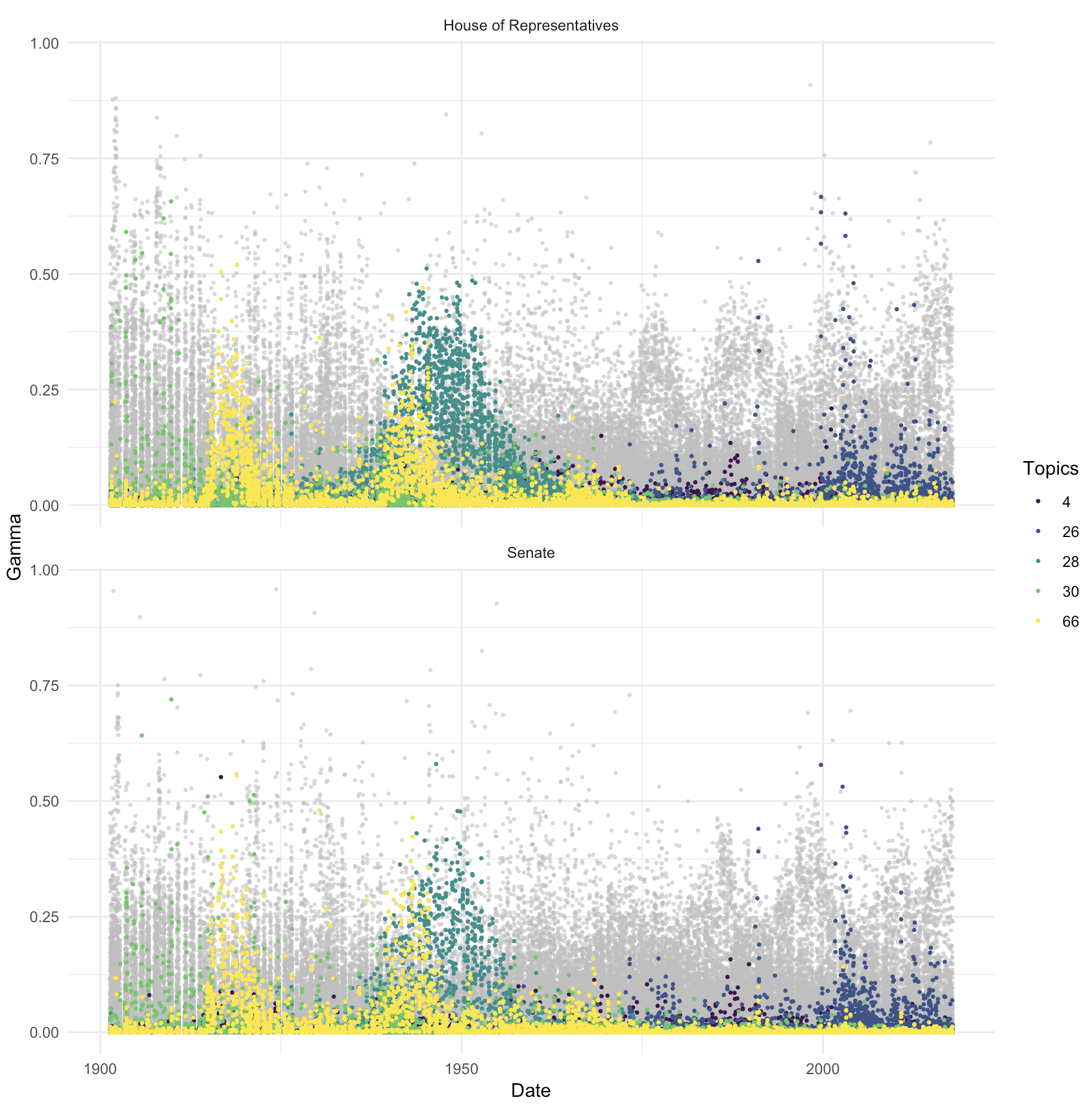
Figure 1: Illustrative topic model output, with five topics highlighted

Figure 2 shows the topic model output in the context of three notable periods of Australian political history. The first panel of Figure 2 is the second Menzies term. The dashed lines show the elections. While the results here abstract from differences based on topic mix, the shape of the distribution seems to be reasonably similar. Given 80 topics, it may be difficult to see differences in the topic mix manually, and so we would like for the analysis model to be able to suggest whether the mix is changing. The second panel shows the 1983 election, and the subsequent change from Fraser to Hawke on 11 March 1983, identified by a dotted line on that date. The distribution of topics seems less bunched after the change, but it is difficult to tell how different it is. We would like the analysis model to be able to distinguish between the two if they seem different. The third panel shows the first Rudd term. The important aspect to note is that the period after the 2007 election and the Rudd term contain essentially the same Hansard dates. The analysis model needs to be able to deal with this situation.

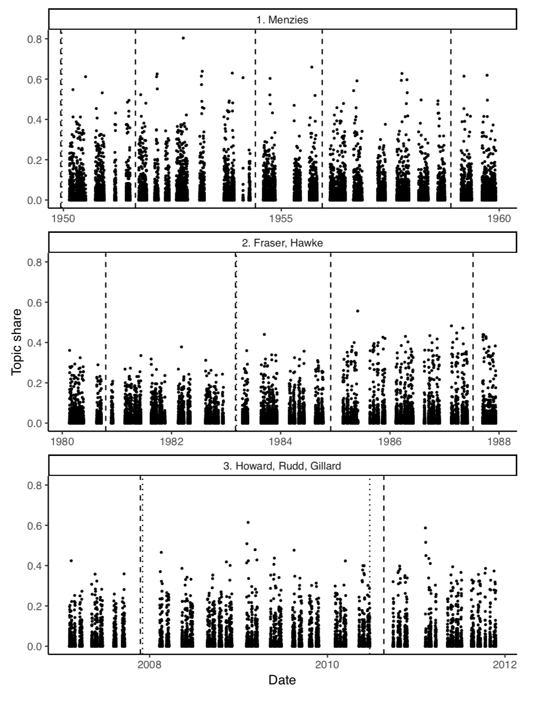
Figure 2: Illustrative topic model output, for three periods

Results from analysis model

As discussed in Section 3.2, the modelling process takes the topic proportions estimated by the CTM and reduced to the Comparative Agendas Project, and examines the association between these topic distributions and events.

There are several outputs of interest from this modelling stage. For example, the model provides estimates of topic prevalence by each sitting period. Figure 3 illustrates the estimated topic prevalence by sitting period for topic 15, one of the defense-related topics, overlaid with the daily topic prevalence (as also illustrated in Figure 2 above). This nicely illustrates how the topics change over time, as the daily estimates tend to be quite variable.

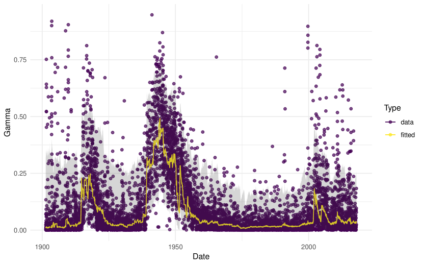
Figure 3: Model estimates of topic prevalance by sitting period for those related to war and conflict

One of the main goals of the analysis model is to see which elections and changes of prime minister are associated with changes in the prevalence of topics over time. By way of background, as Australia has a parliamentary system it is possible for the prime minister to change without an election. If a person was prime minister more than once then these periods are considered independently.

As detailed in Section 3.2, the model estimates an effect for each prime minister, $\alpha_{\_}g$ and each election, $\beta_{\_}e$. We identify differences between neighbouring prime ministers and between neighbouring elections based on calculating 95 per cent Bayesian credible intervals from posterior samples of these respective mean effects. When these do not overlap we consider that the model finds a difference between either the neighbouring prime ministers or elections, as appropriate.

We summarise our results in terms of prime ministers in Table 2 and in terms of elections in Table 3. These tables focus on prime ministers and elections that were different to the ones that preceded them. A total of 17 out of the 36 prime ministerial periods had significantly different topic discussions than their predecessor. In terms of elections, 12 out of a total of 45 elections were significantly different to the previous cycle.

Table 2: Prime ministers that were significantly different to their predecessor

Number	Premiership	Start	End	Party changed
2	Deakin 1	1903-09-24	1904-04-27	No
3	Watson	1904-04-27	1904-08-18	Yes
6	Fisher 1	1908-11-13	1909-06-02	Yes
9	Cook	1913-06-24	1914-09-17	Yes
12	Bruce	1923-02-09	1929-10-22	Yes
14	Lyons	1932-01-06	1939-04-07	Yes
17	Fadden	1941-08-28	1941-10-07	Yes
20	Chifley	1945-07-13	1949-12-19	No
22	Holt	1966-01-26	1967-12-19	No
24	Gorton	1968-01-10	1971-03-10	Yes
25	McMahon	1971-03-10	1972-12-05	No
28	Hawke	1983-03-11	1991-12-20	Yes
29	Keating	1991-12-20	1996-03-11	No
31	Rudd 1	2007-12-03	2010-06-24	Yes
32	Gillard	2010-06-24	2013-06-27	No
34	Abbott	2013-09-18	2015-09-15	Yes
35	Turnbull	2015-09-15	2018-08-24	No

• Note:

• The significance of a prime minister is determined by whether at least one topic was significantly different during this term, compared with the previous one.

Table 3: Election-periods that were significantly different to the one before

Number	Year	Date	Total seats	Election winner	Changed party
9	1922	1922-12-16	75	Non-labor	No
19	1949	1949-12-10	121	Non-labor	Yes
20	1951	1951-08-28	121	Non-labor	No
22	1955	1955-12-10	122	Non-labor	No
24	1961	1961-12-09	122	Non-labor	No
25	1963	1963-11-30	122	Non-labor	No
29	1974	1974-05-18	127	Labor	No
33	1983	1983-03-05	125	Labor	Yes
34	1984	1984-12-01	148	Labor	No
38	1996	1996-03-02	148	Non-labor	Yes
43	2010	2010-08-21	150	Labor	No
45	2016	2016-07-02	150	Non-labor	No

• Note:

• The significance of an election is determined by whether at least one topic was significantly different during the period between this election and the next, compared with the period between the previous election and this one.

In Figures 4 and 5 we focus on certain topics to illustrate significant differences between prime ministers and elections, respectively. In the graphs, the points show the estimated value of $\alpha_{\_}g$ and $\beta_{\_}e$, respectively, for each of the topics specified. The error bars represent 95 per cent Bayesian credible intervals. We have focused on Topics 1, 2, 7, 13, 15, 16, 17, and 19 here which have to do with war and conflict. Large differences can be seen at various times.

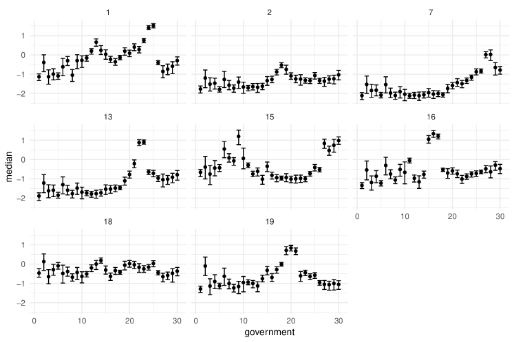
Figure 4: Level effects for prime ministers by selected topics.

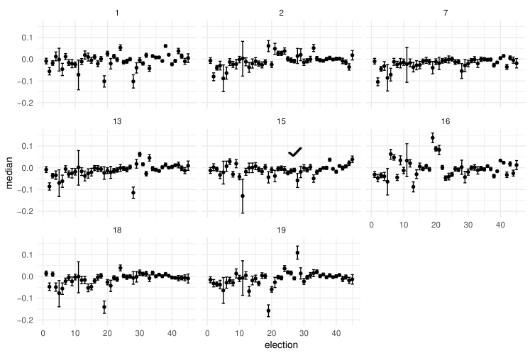
Figure 5: Level effects for election periods by selected topics

Additional results: identifying outlying days

Once prime minister and election effects have been taken into consideration, some days stand out compared with others in their sitting period. We do not explicitly include them in the model because of over-fitting and effect-type concerns, but we are interested to see if these can be explained by events that occurred on or before that sitting day. For instance, we may expect that events of a historical magnitude, such as the 9/11 attacks would change the discussion, or that the sitting day when, for instance, the Apology to the Stolen Generation was delivered, or some particularly prominent legislation introduced, would be different to others in that sitting period.

The model set-up allows for these outlying days to be identified. In particular, we are estimating $\mu_{\_}{c,s,p}$, which can be thought of as the mean topic prevalence for topic $p$ in chamber $c$ and sitting period $s$. We can identify ‘outlying days’ by comparing this mean prevalence and a particular day’s topic distribution. This approach means that the model generates dates that are interesting without us having to specify interesting dates. More specifically, we define a day to be ‘outlying’ or ‘different-to-expected’ if the topic distribution on that particular day is more than three standard deviations different to the mean topic distribution for the relevant sitting period.

Table 4 summarises the days where parliamentary discussion was significantly different from the rest prevailing in that week. Notably, considerably more than a majority of these dates occur in the first half of our sample. And a full seven occur in 1909.

Table 4: Days that were significantly different to other days in their sitting period

Dates
1904-07-15	1911-12-13	1930-06-06	1945-05-30	1991-01-22	2002-08-26
1908-10-30	1912-10-02	1930-06-11	1945-06-12	1999-09-21	2003-03-20
1909-10-13	1912-10-18	1930-06-12	1946-11-06	1999-09-22	2003-05-13
1909-10-14	1923-07-27	1935-10-09	1947-11-14	1999-09-23	2006-02-16
1909-10-19	1923-07-30	1935-11-06	1949-02-22	1999-09-27	2010-03-16
1909-10-20	1923-07-31	1935-11-07	1954-02-15	2001-03-08	2012-10-30
1909-10-21	1923-08-01	1944-03-17	1959-03-12	2001-05-09	2013-06-25
1909-10-22	1925-08-26	1944-07-17	1965-05-26	2001-09-17	2015-11-30
1909-10-26	1927-10-19	1945-04-18	1991-01-21	2002-06-04	-

• Note:

• These days were significantly different to others in their sitting period after taking election and prime minister effects into consideration.

Discussion

In this paper we explored changes in parliamentary discussion in association with changing prime minister and elections events in Australia. We used OCR and other text processing techniques to create a comprehensive dataset which covers parliamentary discussion in Australia throughout history since Federation in 1901 to the present day. We then used topic modeling to ascertain comparable topics of discussion over time, and a Bayesian hierarchical Dirichlet model to relate these topics to changes in elections and prime ministers. In general we find that changes in prime minister change the distribution of topics discussed in parliament, but that most elections did not. We find that significant events such as 9/11 and the Bali Bombings had a substantial effect.

Of the 36 prime ministers over this period, we find that 17 of them were significantly different to the prime minister that preceded them, after we account for and remove some that had especially short terms. The three earliest of them occur in the first decade after Federation, and to a certain extent this may be due to the variety of the issues that had to be addressed in those initial years. Joseph Cook’s time as prime minister is found to be significantly different to that of his predecessor, Andrew Fisher, although it may be that this is due to World War I.

The second Menzies term, beginning in 1949, is the next government that is significantly different to its predecessor. The other governments that are different are concentrated in the second half of our sample, with three of them being in the past twenty years. Similarly, of the 45 general elections that have been held we find that 14 of them define periods that were significantly different to their immediate predecessor. 1974, 1980, 1990, 1998, 2004, and 2007 stand out as elections where the government did not change, but the model suggests there was considerable change in the topics discussed in parliament.

The second Menzies term was associated with a variety of changes compared with the preceding Chifley Government. Chifley had governed through the end of World War II and the difficult economic times that followed. There was also a large increase in the number of seats in the House of Representatives at the 1949 election. Many new politicians entered parliament, and this changed representation may also have been partly to do with the changed distribution of discussion topics, although further investigation of this is left for future work. The sixteen-year length of the second Menzies term, and better economic conditions over this time make it understandable why parliamentary discussion would have been different. There were six elections within the second Menzies term. Three toward the middle of that government were associated with significant changes in the topics discussed.

Menzies was succeeded by Holt in January 1966. This is an example where there was a change in prime minister without an election, as the next election only happened in November 1966. We find that Holt is different to Menzies.

In Figures 6 we compare the topics during Menzies’ final term with the topics of Holt.

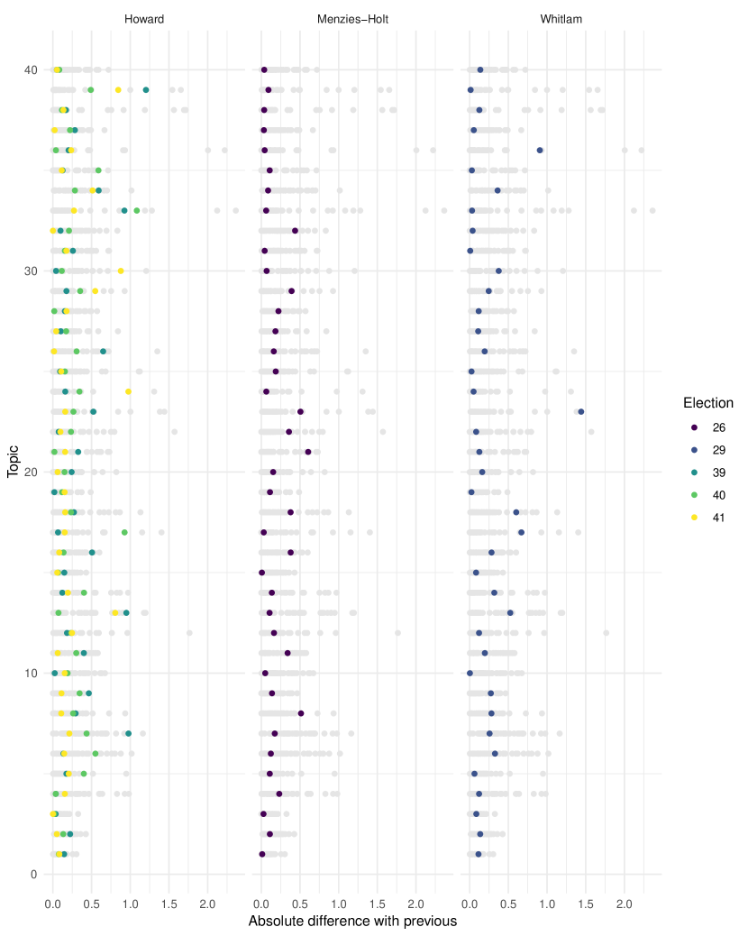
Figure 6: Differences between various elections

Whitlam’s term is especially interesting as we find a difference in the topics after he was first elected in December 1972, compared with his second election win in May 1974. Figure 6 compares the topics that are significant before and after the election.

Howard is also interesting because of the significant differences between elections. For instance, each of the election periods is associated with fairly substantial differences compared with the preceding election periods, and all are actually significantly different at the 95 per cent level. Figure 6 compares the topics that are significant in the different elections that Howard won.

To a certain extent the change after the November 2001 election is expected because of the 9/11 terrorist attacks that had only occurred two months earlier, the Bali Bombings that occurred in October 2002, and the dramatic increase in the discussion related to terrorism and conflict over these years. However, the change in 1998 and 2004 is more unexpected. Although Howard is the second-longest serving prime minister and commonly thought of as a period of stability because the senior ministers were consistent as well, it might be that it is better to think of Howard as a combination of three or four different periods and that Howard reinvented itself over this period.

One advantage of our analysis model compared with using the STM approach is that we can create a measure that is equivalent to testing for outliers in a model where the underlying variables were not latent. The results of this reduction in supervision are promising, but suggest the specifics of our process may need further refinement. For instance, our approach appropriately identifies the sitting day that first follows 11 September 2001. But there are many dates that we would have expected to be identified that were not, and similarly some of the dates that were identified are surprising. When we examine this we find that some of them are associated with significant legislation. Although our results are not overly over-weighted in the first half of our sample, there is a substantial gap between 1965 and 1991. Table 4 highlights further work is needed to improve this approach. For instance, it may be that our approach is not appropriately considering step-changes or it may be that our identification of sitting periods is not appropriate for the entire period, given the changed sitting pattern that we identify.

Limitations and future work

Using text as data allows us to conduct larger-scale analysis that would not be viable using less-automated approaches and so researchers may be able to identify associations and patterns that would otherwise have been overlooked. That said, the approach has well-known shortcomings and weaknesses, such as those documented by Grimmer and Stewart (2013). Because of these, our paper should be considered a complement to more detailed analysis such as qualitative methods and case studies.

One weakness of topic models is that the number of topics needs to be specified but there is rarely a clear reason to choose some particular number. There are also more nuanced weaknesses to be aware of. For instance, the topics need to be interpreted. Some of our topics were not overly meaningful, especially on their own. Interpretation is especially difficult when the number of topics is large, but we found that a large number of topics worked best for our dataset.

Although topic modelling is an unsupervised machine learning technique, the inputs require fine-tuning. For instance, selecting stop words for removal and which words to merge because of common co-location has an impact on the topics. Topic model outcomes are known to be sensitive to preprocessing (Denny and Spirling, 2018) and ours was no exception.

One way to get around using topic models is to use a supervised learning approach, such as that used by Ash, Morelli and Osnabru (2018) in the context of New Zealand Hansard. Another is to use the words more directly, for instance word2vec and other approaches. As computational power become cheaper and more appropriate analytical methods, such as Taddy (2015) as applied in Gentzkow, Shapiro and Taddy (2018) in the context of examining congressional speech records, are developed this becomes a more feasible options and future research could explore that direction.

In this paper we think of events as affecting daily discussion in parliament. Given the events that we consider and the broad topics of discussion we consider this the most appropriate direction for our paper. However, conducting a similar analysis at a person, instead of daily, level would lead to interesting results. This would allow the analysis model to include a rich set of person-level covariates such as gender or party, and account for broader factors such as the televising of question time, or the state of the economy and the budget position. It would also be especially interesting to consider reversing the direction of causality and examine the effect of what is said in parliament on various economic, political and social events.

In terms of the analysis model that relates the topic distributions with events, there are several limitations to the model. Firstly, we are assuming that the effect of a particular prime minister is constant across the whole period. In addition, we assume that the effect of elections is monotonically decreasing across days since election. Future work could consider different functional forms on both of these effects, and in particular try to allow for elections to have a ‘lead-up’ effect.

The way that we identify unusual periods could also be improved. We defined sitting periods in a constant fashion across the whole dataset time frame, but how long the stretches are that parliament sits for has changed over time. In addition, more work needs to be done on how to identify outlying events. For instance, the extent to which an important event that occurs outside a sitting period can be identified has a great deal of uncertainty. And if an event happens in the middle of a sitting period, it may have a large effect on the overall mean, such that specific days are not identified as significantly outlying.

Finally, the current modelling and analysis set-up is a two-stage process: we take the output of a topic model, and use this as the input to a second model. However, this approach does not appropriately propagate the uncertainty of the topic distribution estimation stage. Future methodological work could consider how to combine these two modelling steps, for instance by extending the STM approach into a more flexible framework.

Watching Australian politicians at work can sometimes be a little disheartening. It can be hard to believe that not only are those in charge shouting insults that would not be tolerated in a schoolyard, but that the electorate voted to put them there. Nonetheless, our work suggests that important topics are discussed in parliament. It is easy to look back and think that we live in uniquely tumultuous times, but our analysis suggests events have always driven debate and that periods of stability may be the exception. However, we do find that since the 1990s the effect of prime ministers and elections on the topics discussed in the Australian parliament does seem more pronounced than it used to be.

Appendix

Authors: Rohan Alexander and Monica Alexander

Appendix A Hansard details

Example Hansard page

Figure 7: Example Hansard page – 6 February 1902

Summary statistics

Counts per year

The number of sitting days in a year varies considerably. The highest in the House of Representatives was 122 days in 1904, followed by 113 days in 1901 and 1920. The year with the most sitting days in the Senate was 1902 with 93 days, followed by 1989 with 92 days, and 1986 with 86 days (Figure 8).

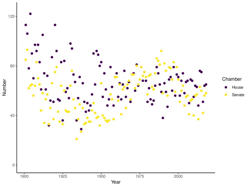
Figure 8: Number of sitting days, by year

Until the 1950s the House of Representatives tended to have more sitting days than the Senate. It was then similar, before the Senate had more days in the 1980s and 1990s. Since the 2000s the House of Representatives again has tended to have more sitting days than the Senate.

Distribution over the year

The distribution of sitting days over the course of the year changes over time (Figure 9).

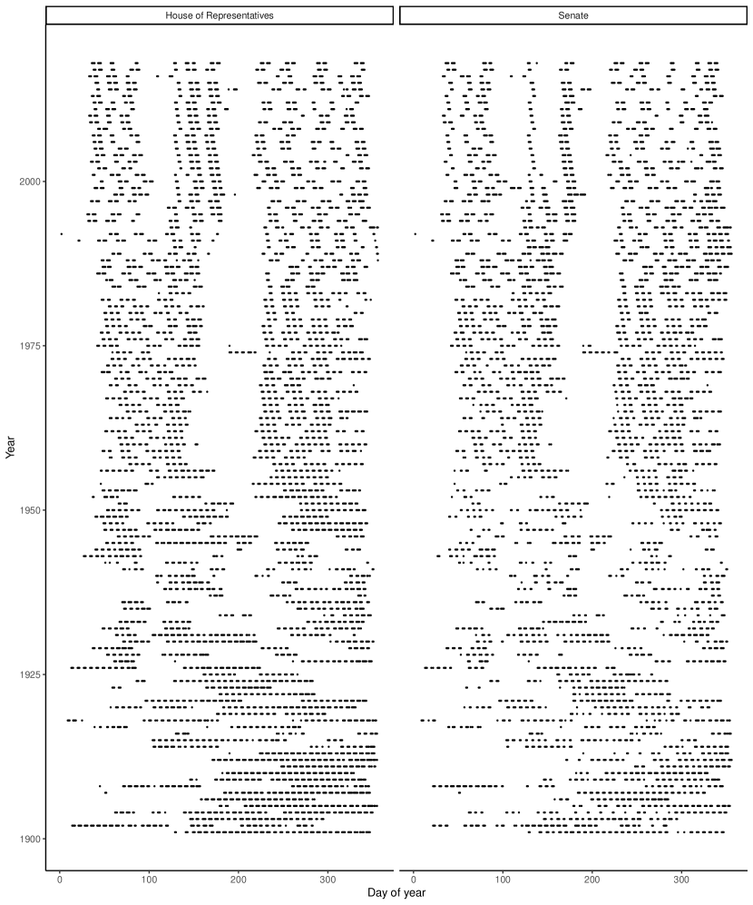
Figure 9: All sitting days

It was initially more piecemeal. This can be seen by comparing the pattern of sitting days in the years to 1920 (Figure 10) with those in the 19 years from, and including, 2000 (Figure 11).

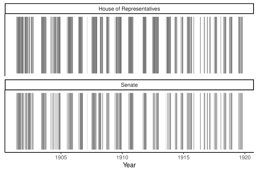
Figure 10: Number of sitting days, by year

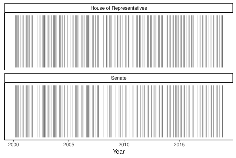
Figure 11: Number of sitting days, by year

The largest gap between sitting dates for both the House of Representatives and the Senate is 284 days, which happened when neither house sat between 25 November 1910 and 5 September 1911. The next longest gap is 244 the House of Representatives and 243 for the Senate when the lower house last sat on 9 October 1924, the upper house last sat on 10 October 1924 and neither sat again until 10 June 1925.

These counts of the number of sitting days are based on available PDFs. For this reason the counts may be slightly different to other counts. An example of one known issue of this type is detailed in the next section.

Annual counts of sitting days, compared with parliamentary website

The parliamentary website provides a summary table of the number of sitting days in each year by chamber. Comparing the numbers provided in that table with number of days that we have provides an indication of how complete our dataset is.

In general the number of sitting days on the parliamentary website summary table is similar to the number of PDFs that we have although it does identify a few particularly concerning years (Figure 12).

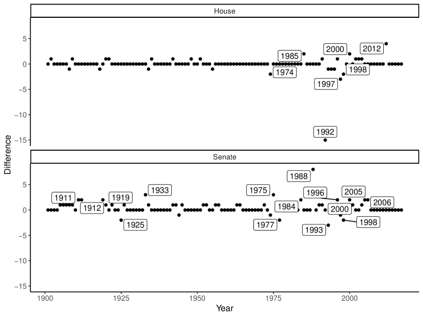
Figure 12: Differences by year between the number of sitting days and our number of PDFs

When the difference is positive, it means that in that year we have fewer PDFs than the parliamentary website claims. For instance, 5 could mean that the parliamentary website claimed there were 100 days, but we only had PDFs for 95 days. Similarly, when the difference is negative then we have more PDFs than the parliamentary website claims there were sitting days.

The two major years of concern are 1992 in the House of Representatives where we have 15 days more than the parliamentary website claims there were, and 1988 in the Senate where we have eight days fewer. We examined the physical copy of the Hansard kept in the NSW State Library and this suggests that the summary table on the parliamentary website may be wrong.

The Parliament website is missing the Hansard PDFs for the following dates in the Senate: 1988-12-21, 1988-12-20, 1988-12-19, 1988-12-16, 1988-12-15, 1988-12-14, 1988-12-13, 1988-12-12, 2000-10-12, 2000-06-19, and 2004-08-09.

There are two unaccounted for differences in 2006, one unaccounted for difference in 2001.

The Parliament website is missing the Hansard PDFs for the following dates in the House of Representatives: 1985-08-23, 1992-09-10, 1996-12-13, 2000-10-12, 2000-06-29, and 2002-05-14.

There is one unaccounted for difference in 1920, 1921, 1935, 1942, 1948, 1951, 1991, 2003, 2004, and there are two unaccounted for in 1985 and four unaccounted for in 2012.

In terms of other known issues, in the Senate, the PDF for the website date 10 August 1917 may be wrong. When downloaded the PDF says that it is for 10 January 1918 on the cover sheet, but there’s no website entry for 10 January 1918. This is also the case for 18 December 1918 (which contains the PDF for 28 November 1918), and for 1 August 1917 (which contains the PDF for 10 August 1917).

Stopwords over time

Figure 13 shows the proportion of five common words – ‘and’, ‘be’, ‘of’, ‘the’, ‘to’ – compared with the total number of words over time.

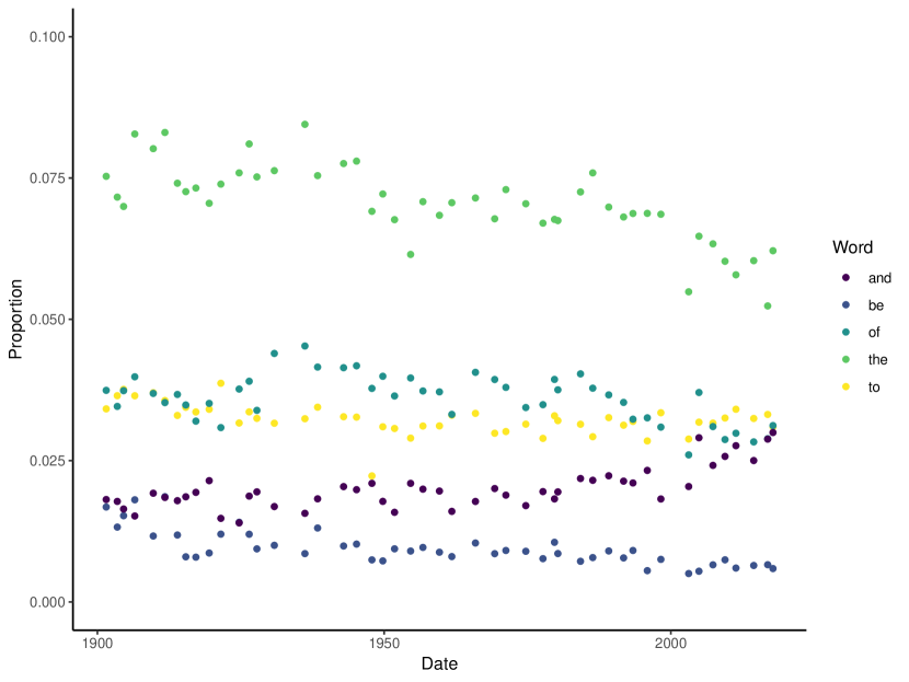
Figure 13: Proportion that some common words comprise of all words, over time

Appendix B Topic modelling example and details

Overview and example

As applied to Hansard, LDA considers each statement to be a result of a process where a politician first chooses the topics they want to speak about. After choosing the topics, the politician then chooses appropriate words to use for each of those topics. Statistically, LDA considers each document as having been generated by some probability distribution over topics. Similarly, each topic is considered a probability distribution over terms. To choose the terms used in each document, terms are picked from each topic in the appropriate proportion.

As an example, Figures 14 and 15 illustrate a smaller application with five topics, two documents, and ten terms. In this case, the first document may be comprised mostly of the first few topics; the other document may be mostly about the final few topics (Figure 14).

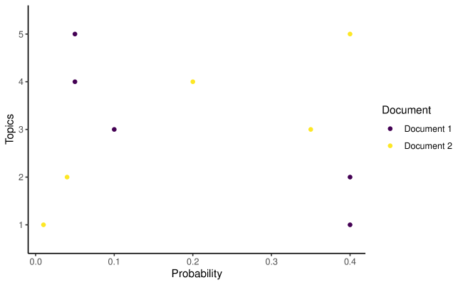
Figure 14: Probability distributions over topics for two documents

For instance, if there were ten terms, then one topic could be defined by giving more weight to terms related to immigration; and some other topic may give more weight to terms related to the economy (Figure 15).

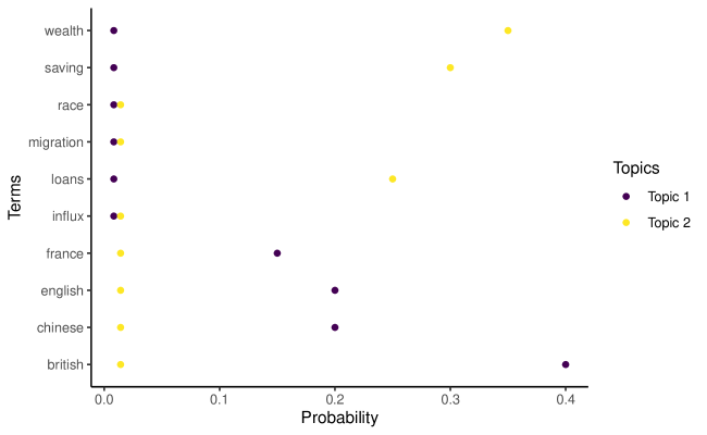
Figure 15: Probability distributions over terms

Document generation process

Following Blei and Lafferty (2009), Blei (2012) and Griffiths and Steyvers (2004), the process by which a document is generated is more formally considered to be:

1. There are $1,2,\dots,k,\dots,K$ topics and the vocabulary consists of $1,2,\dots,V$ terms. For each topic, decide the terms that the topic uses by randomly drawing distributions over the terms. The distribution over the terms for the $k$th topic is $\beta_{\_}k$. Typically a topic would be a small number of terms and so the Dirichlet distribution with hyper-parameter $\boldsymbol{\eta}$ is used: $\beta_{\_}k\sim\mbox{Dirichlet}(\boldsymbol{\eta})$, where $\boldsymbol{\eta}=(\eta_{\_}1,\eta_{\_}2,\dots,\eta_{\_}{K})$. In practice, a symmetric Dirichlet distribution is usually used, where all elements of $\boldsymbol{\eta}$ are equal.

2. Decide the topics that each document will cover by randomly drawing distributions over the $K$ topics for each of the $1,2,\dots,d,\dots,D$ documents. The topic distributions for the $d$th document are $\theta_{\_}d$, and $\theta_{\_}{d,k}$ is the topic distribution for topic $k$ in document $d$. Again, the Dirichlet distribution with the hyper-parameter $0<\alpha<1$ is used here because usually a document would only cover a handful of topics: $\theta_{\_}d\sim\mbox{Dirichlet}(\boldsymbol{\alpha})$. Again, strictly $\boldsymbol{\alpha}$ is vector of length $K$ of hyper-parameters and they are usually equal.

3. If there are $1,2,\dots,n,\dots,N$ terms in the $d$th document, then to choose the $n$th term, $w_{\_}{d,n}$:

   1. Randomly choose a topic for that term $n$, in that document $d$, $z_{\_}{d,n}$, from the multinomial distribution over topics in that document, $z_{\_}{d,n}\sim\mbox{Multinomial}(\theta_{\_}d)$.

   2. Randomly choose a term from the relevant multinomial distribution over the terms for that topic, $w_{\_}{d,n}\sim\mbox{Multinomial}(\beta_{\_}{z_{\_}{d,n}})$.

Given this set-up, the joint distribution for the variables is (Blei (2012), p.6):

$$p(\beta_{\_}{1:K},\theta_{\_}{1:D},z_{\_}{1:D,1:N},w_{\_}{1:D,1:N})=\prod^{K}_{\_}{i=1}p(\beta_{\_}i)\prod^{D}_{\_}{d=1}p(\theta_{\_}d)\left(\prod^{N}_{\_}{n=1}p(z_{\_}{d,n}|\theta_{\_}d)p\left(w_{\_}{d,n}|\beta_{\_}{1:K},z_{\_}{d,n}\right)\right).$$

Based on this document generation process the analysis problem, discussed next, is to compute a posterior over $\beta_{\_}{1:K}$ and $\theta_{\_}{1:D}$, given $w_{\_}{1:D,1:N}$. This is intractable directly, but can be approximated (Griffiths and Steyvers (2004) and Blei (2012)).

After the documents are created, they are all that we have to analyse. The term usage in each document, $w_{\_}{1:D,1:N}$, is observed, but the topics are hidden, or ‘latent’. We do not know the topics of each document, nor how terms defined the topics. That is, we do not know the probability distributions of Figures 14 or 15. In a sense we are trying to reverse the document generation process – we have the terms and we would like to discover the topics.

If the earlier process around how the documents were generated is assumed and we observe the terms in each document, then we can obtain estimates of the topics (Steyvers and Griffiths (2006)). The outcomes of the LDA process are probability distributions and these define the topics. Each term will be given a probability of being a member of a particular topic, and each document will be given a probability of being about a particular topic. That is, we are trying to calculate the posterior distribution of the topics given the terms observed in each document (Blei (2012), p. 7):

$$p(\beta_{\_}{1:K},\theta_{\_}{1:D},z_{\_}{1:D,1:N}|w_{\_}{1:D,1:N})=\frac{p\left(\beta_{\_}{1:K},\theta_{\_}{1:D},z_{\_}{1:D,1:N},w_{\_}{1:D,1:N}\right)}{p(w_{\_}{1:D,1:N})}.$$

Gibbs sampling or the variational expectation-maximization algorithm can be used to approximate the posterior. A summary of these approaches is provided next.

Posterior estimation

Following Steyvers and Griffiths (2006) and Darling (2011), the Gibbs sampling process attempts to find a topic for a particular term in a particular document, given the topics of all other terms for all other documents. Broadly, it does this by first assigning every term in every document to a random topic, specified by Dirichlet priors with $\alpha=\frac{50}{K}$ and $\eta=0.1$ (Steyvers and Griffiths (2006) recommends $\eta=0.01$), where $\alpha$ refers to the distribution over topics and $\eta$ refers to the distribution over terms (Grün and Hornik (2011), p. 7). It then selects a particular term in a particular document and assigns it to a new topic based on the conditional distribution where the topics for all other terms in all documents are taken as given (Grün and Hornik (2011), p. 6):

$$p(z_{\_}{d,n}=k|w_{\_}{1:D,1:N},z^{\prime}_{\_}{d,n})\propto\frac{\lambda^{\prime}_{\_}{n\rightarrow k}+\eta}{\lambda^{\prime}_{\_}{.\rightarrow k}+V\eta}\frac{\lambda^{\prime(d)}_{\_}{n\rightarrow k}+\alpha}{\lambda^{\prime(d)}_{\_}{-i}+K\alpha}$$

where $z^{\prime}_{\_}{d,n}$ refers to all other topic assignments; $\lambda^{\prime}_{\_}{n\rightarrow k}$ is a count of how many other times that term has been assigned to topic $k$; $\lambda^{\prime}_{\_}{.\rightarrow k}$ is a count of how many other times that any term has been assigned to topic $k$; $\lambda^{\prime(d)}_{\_}{n\rightarrow k}$ is a count of how many other times that term has been assigned to topic $k$ in that particular document; and $\lambda^{\prime(d)}_{\_}{-i}$ is a count of how many other times that term has been assigned in that document. Once $z_{\_}{d,n}$ has been estimated, then estimates for the distribution of words into topics and topics into documents can be backed out.

This conditional distribution assigns topics depending on how often a term has been assigned to that topic previously, and how common the topic is in that document (Steyvers and Griffiths (2006)). The initial random allocation of topics means that the results of early passes through the corpus of document are poor, but given enough time the algorithm converges to an appropriate estimate.

The choice of the number of topics, k, drives the results and must be specified a priori. If there is a strong reason for a particular number, then this can be used. Otherwise, one way to choose an appropriate number is to use cross validation. More detail on this process is provided in the next section.

Selection of number of topics

The choice of the number of topics to use in a topic model has a substantial effect on the results of the model. For instance, in our topic model, choosing a smaller number of topics, such as 10 or 20 results in a model that is not all that useful because the topics are so broad.

There are a variety of diagnostic measures that can guide the selection of the topics, but there is rarely a clear best choice, especially at a finer level such as choosing between 60 and 65 topics. We found it useful to try a few quite different measures before settling on 80 topics. This provided a balance between being granular enough to be informative—anything less than 40 topics tended to be too broad—yet still being tractable for our analysis model in a reasonable amount of time. In addition to looking at the topics and how they changed over time, diagnostic measures that we considered include the held-out likelihood, the lower bound, residuals, exclusivity. and semantic coherence (Figures 16).

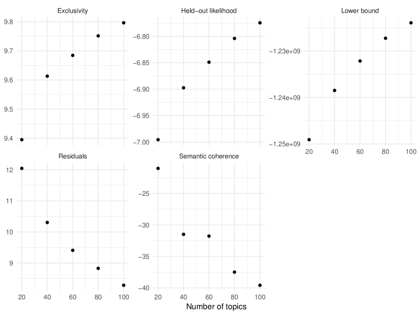
Figure 16: Model diagnostics

Roberts, Stewart and Tingley (2018) provides more detail about the diagnostic tests that we use, but we briefly discuss each here. Exclusivity is a measure of how specific words are to particular topics. It looks at the proportion that a word makes up of a particular topic compared with the proportion that word makes up of the other topics. As the number of topics increases we usually expect exclusivity to increase because the topics become more particular. Higher values are better. The held-out likelihood as described by Wallach et al. (2009) takes a test/training approach to estimate the probability of held-out documents given the training documents. Higher values are better. The lower bound gives some indication of whether the model may have multiple modes and hence the end result be sensitive to the starting position (Roberts, Stewart and Tingley (2016)). Residuals analysis, Taddy (2012), compares the theoretical distribution of the variance with the actual distribution. It is a test for over-dispersion of the variance, and if it is found then this can suggest that more topics would be appropriate. Semantic coherence is the trade-off for having topics that are more specific and the subsequent risk that the topics become meaningless. Mimno et al. (2011) define a measure of coherence that is based on ratios of single words compared with pairs of words. The idea is that words that should occur in the one document should be more likely to be in a particular topic than ones that do not occur together. For instance, a topic that has ‘wine’ and ‘cheese’ as highly rated words would score better on their measure than another that contained ‘cheese’ and ‘mining’. Lower values are better. Roberts, Stewart and Tingley (2018) recommend examining the trade-off between exclusivity and semantic coherence. This suggests that the magnitude of improvement reduces from about 80 topics (Figure 17).

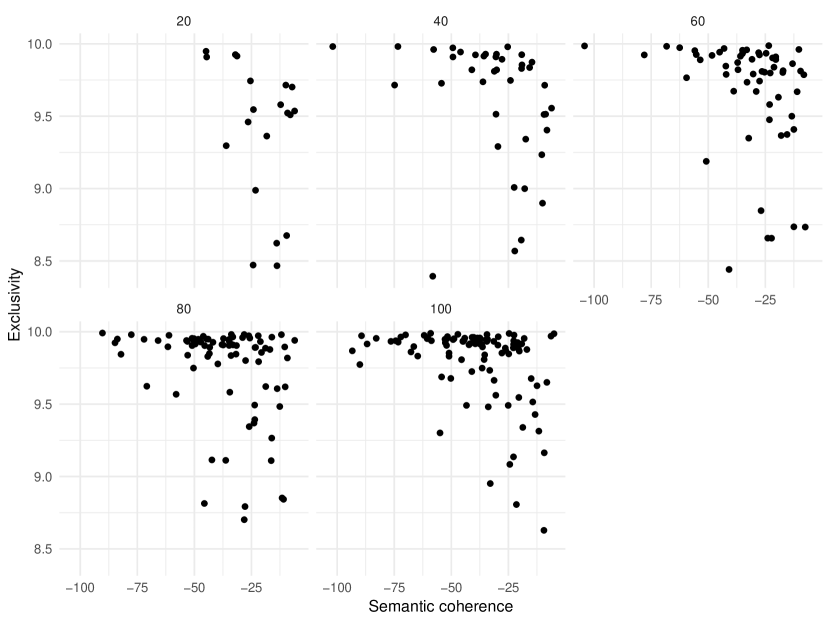
Figure 17: Exclusitivity compared with semantic coherence

Correlated Topic Model

One of the limitations of LDA is that the model assumes that the presence of one topic is not correlated with the presence of another topic. In reality, topics are often related. For instance, in the Hansard context, we may expect topics related to the army to be more commonly found with topics related to the navy, but less commonly with topics related to banking. The goal of the CTM (Blei and Lafferty, 2007) is to account for this correlation between topics, in order to produce more realistic and stable topic distributions over time. The models are very similar, and the key difference is the underlying distributions that are drawn from.

As with LDA, the process assumed to generate the documents is the key aspect as this will be reversed to estimate the topics. The document generation process of Blei, Ng and Jordan (2003), discussed in Appendix B.2, is just slightly modified. Specifically, rather than assuming that the distribution of topics in a document, $\theta_{\_}d$, are a draw from a Dirichlet distribution, as in Step 2 of the LDA document generation process detailed in Appendix B.2, CTM assumes:

$$\theta_{\_}d\sim\mbox{Logistic Normal}(\mu,\Sigma).$$

That is, the main difference of CTM over LDA is that it replaces the assumption of the Dirichlet distribution with a more flexible logistic multivariate Normal distribution. This distribution can incorporate a covariance structure across the topics. The remainder of the steps of the document generating process are pretty much the same as LDA.

However, the replacement of the Dirichlet distribution with the logistic multivariate Normal distribution adds a level of computational complexity to CTM. The posterior distributions of the parameters of interest ($\beta_{\_}{1:K},\theta_{\_}{1:D},z_{\_}{1:D,1:N}$) can no longer be obtained using standard simulation techniques such as Gibbs Sampling. Blei and Lafferty (2007) develop a fast variational inference procedure for estimating the CTM. CTM itself has also been extended by Roberts, Stewart and Airoldi (2016) as part of their work on Structural Topic Models. The main difference is to add a covariate to $\mu$ which allows consideration of additional information.

Appendix C Topic model outputs - Economics

Although the example topics in the main paper have a military and defence theme, there are other topics that also share a broader theme. An example of these are those to do with economics. For instance Topics 17, 22, 25, 44, 51, 55, 59, 71, 72, 74, 76, and 77.

In Figure 18 we focus on the period around the Great Depression and the Premiers’ Plan.

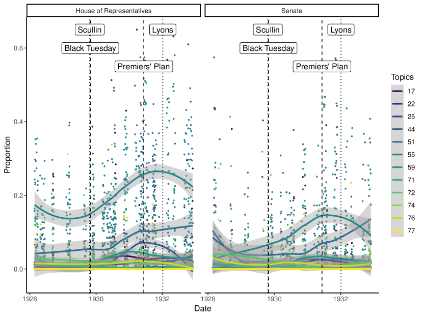
Figure 18: Economic topic changes around the the Great Depression

The notable aspect of the response to the 1929 ‘Black Tuesday’ stock market declines was the Premiers’ Plan, which appeared newspapers on 11 June 1931. Copland (1934) describes the differences of opinion that occurred in the lead-up to the plan, but Figure 18 highlights how new the Scullin Government was when the economic troubles began.

In Figure 19 we focus on the 1980s and 1990s when there was a great deal of economic change.

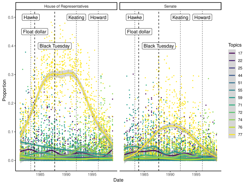
Figure 19: Economic topic changes during the 1980s and 1990s

One notable aspect is the difference between the House of Representatives and the Senate that the proportion of economic topics accounts for. The emphasis that the Hawke/Keating government placed on economic issues comes through clearly given the clear change following Hawke’s election.

Finally, in Figure 20 we focus on the financial crisis of 2007-08.

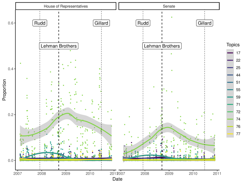
Figure 20: Economic topic changes around the 2007-08 financial crisis

It is notable that despite the enormous importance of the financial crisis of 2007-08, topics that are clearly related to economic issues do not dominate the discussion in either house.

Appendix D Events

List of Elections

The first of the two types of events that we consider in this paper is an election (Table LABEL:tab:elections).

[para]

Note:

This table contains summary information for each prime minister of Australia. HoR and Senate refer to the number of days that each chamber sat for between elections.

Table 5: List of Australian elections

Number	Year	Date	Total seats	Winner	HoR	Senate
1	1901	1901-03-29	75	Non-labor	297	240
2	1903	1903-12-16	75	Non-labor	282	185
3	1906	1906-12-12	75	Non-labor	286	217
4	1910	1910-04-13	75	Labor	249	167
5	1913	1913-05-31	75	Non-labor	108	59
6	1914	1914-09-05	75	Labor	147	133
7	1917	1917-05-05	75	Non-labor	174	134
8	1919	1919-12-13	75	Non-labor	258	197
9	1922	1922-12-16	75	Non-labor	171	132
10	1925	1925-11-14	75	Non-labor	205	147
11	1928	1928-11-17	75	Non-labor	40	29
12	1929	1929-10-12	75	Labor	206	154
13	1931	1931-12-19	75	Non-labor	155	111
14	1934	1934-09-15	74	Non-labor	169	116
15	1937	1937-10-23	74	Non-labor	153	108
16	1940	1940-09-21	74	Non-labor	144	113
17	1943	1943-08-21	74	Labor	206	132
18	1946	1946-09-28	74	Labor	278	119
19	1949	1949-12-10	121	Non-labor	107	87
20	1951	1951-08-28	121	Non-labor	173	99
21	1954	1954-05-29	121	Non-labor	94	65
22	1955	1955-12-10	122	Non-labor	190	147
23	1958	1958-11-22	122	Non-labor	200	194
24	1961	1961-12-09	122	Non-labor	119	106
25	1963	1963-11-30	122	Non-labor	196	170
26	1966	1966-11-26	124	Non-labor	179	185
27	1969	1969-10-25	125	Non-labor	208	209
28	1972	1972-12-02	125	Labor	97	96
29	1974	1974-05-18	127	Labor	117	118
30	1975	1975-12-13	127	Non-labor	147	151
31	1977	1977-12-10	124	Non-labor	188	196
32	1980	1980-10-18	125	Non-labor	121	152
33	1983	1983-03-05	125	Labor	101	124
34	1984	1984-12-01	148	Labor	183	202
35	1987	1987-07-11	148	Labor	158	215
36	1990	1990-03-24	148	Labor	163	216
37	1993	1993-03-13	147	Labor	187	213
38	1996	1996-03-02	148	Non-labor	180	196
39	1998	1998-10-03	148	Non-labor	215	214
40	2001	2001-11-10	150	Non-labor	189	161
41	2004	2004-10-09	150	Non-labor	196	163
42	2007	2007-11-24	150	Labor	173	129
43	2010	2010-08-21	150	Labor	179	155
44	2013	2013-09-07	150	Non-labor	190	153
45	2016	2016-07-02	150	Non-labor	156	137

Between 1901 and 2018 there are 45 elections, roughly one every two to three years. All of the election periods have a reasonable number of sitting days within them. The fewest was the election on 17 November 1928, with only 40 sitting days in the House of Representatives and 29 in the Senate, as there was another election almost a year later on 12 October 1929.

The number of seats increases from 74 to 121 at the 10 December 1949 election, having been reasonably consistent to that point. Another large increase in the number of seats, this time from 125 to 148, happens at the 1 December 1984 election.

In the first half of our sample especially, the name of the major opposition party changes. For this reason we distinguish between the Labor Party, and the non-Labor Party in terms of who won the election, that is which party was able to form government.

List of Prime Ministers

The second of the two types of events that we consider in this paper is a change in prime minister (Table LABEL:tab:governments).

[para]

Note:

This table contains summary information for each prime minister of Australia. HoR and Senate refer to the number of days that each chamber sat for while that person was prime minister.

Table 6: List of Australian prime ministers

Government	Prime Minister	Party	Start	End	Died in Office	HoR	Senate
Barton	Edmund Barton	Protectionist	1901-01-01	1903-09-24	No	284	228
Deakin 1	Alfred Deakin	Protectionist	1903-09-24	1904-04-27	No	31	23
Watson	Chris Watson	Labour	1904-04-27	1904-08-18	No	47	18
Reid	George Reid	Free Trade	1904-08-18	1905-07-05	No	60	37
Deakin 2	Alfred Deakin	Protectionist	1905-07-05	1908-11-13	No	334	255
Fisher 1	Andrew Fisher	Labour	1908-11-13	1909-06-02	No	15	14
Deakin 3	Alfred Deakin	Commonwealth Liberal	1909-06-02	1910-04-29	No	94	67
Fisher 2	Andrew Fisher	Labor	1910-04-29	1913-06-24	No	249	167
Cook	Joseph Cook	Commonwealth Liberal	1913-06-24	1914-09-17	No	108	59
Fisher 3	Andrew Fisher	Labor	1914-09-17	1915-10-27	No	90	77
Hughes	Billy Hughes	Labor National Labor and Nationalist	1915-10-27	1923-02-09	No	489	387
Bruce	Stanley Bruce	Nationalist (Coalition)	1923-02-09	1929-10-22	No	416	308
Scullin	James Scullin	Labor	1929-10-22	1932-01-06	No	206	154
Lyons	Joseph Lyons	United Australia (Coalition)	1932-01-06	1939-04-07	Yes	396	279
Page	Earle Page	Country (Coalition)	1939-04-07	1939-04-26	No	2	0
Menzies 1	Robert Menzies	United Australia (Coalition)	1939-04-26	1941-08-28	No	118	87
Fadden	Arthur Fadden	Country (Coalition)	1941-08-28	1941-10-07	No	8	6
Curtin	John Curtin	Labor	1941-10-07	1945-07-05	Yes	223	153
Forde	Frank Forde	Labor	1945-07-06	1945-07-13	No	1	1
Chifley	Ben Chifley	Labor	1945-07-13	1949-12-19	No	357	173
Menzies 2	Robert Menzies	Liberal (Coalition)	1949-12-19	1966-01-26	No	1024	822
Holt	Harold Holt	Liberal (Coalition)	1966-01-26	1967-12-19	Yes	117	111
McEwen	John McEwen	Country (Coalition)	1967-12-19	1968-01-10	No	0	0
Gorton	John Gorton	Liberal (Coalition)	1968-01-10	1971-03-10	No	200	201
McMahon	William McMahon	Liberal (Coalition)	1971-03-10	1972-12-05	No	125	128
Whitlam	Gough Whitlam	Labor	1972-12-05	1975-11-11	No	213	213
Fraser	Malcolm Fraser	Liberal (Coalition)	1975-11-11	1983-03-11	No	457	500
Hawke	Bob Hawke	Labor	1983-03-11	1991-12-20	No	546	681
Keating	Paul Keating	Labor	1991-12-20	1996-03-11	No	246	289
Howard	John Howard	Liberal (Coalition)	1996-03-11	2007-12-03	No	780	734
Rudd 1	Kevin Rudd	Labor	2007-12-03	2010-06-24	No	172	128
Gillard	Julia Gillard	Labor	2010-06-24	2013-06-27	No	179	154
Rudd 2	Kevin Rudd	Labor	2013-06-27	2013-09-18	No	1	2
Abbott	Tony Abbott	Liberal (Coalition)	2013-09-18	2015-09-15	No	143	115
Turnbull	Malcolm Turnbull	Liberal (Coalition)	2015-09-15	2018-08-24	No	179	151
Morrison	Scott Morrison	Liberal (Coalition)	2018-08-24	-	-	24	24

Between 1901 and 2018 30 different people have been prime minister. Four of those—Deakin, Fisher, Menzies and Rudd—returned as prime minister at least once after being replaced, meaning Scott Morrison defines the 36th prime ministerial period.

Three people have died while prime minister: Lyons in 1939, Curtin in 1945, and Holt in 1967. Their respective immediate successors were only prime minister for a short period. As such, we do not consider them when determining the neighbouring prime minister. Specifically, we compare: the first Menzies term with Lyons instead of Page; Chifley with Curtin instead of with Forde; and Gorton with Holt instead of with McEwan.

The other prime ministerial period that we do not consider in this paper is the second Rudd term. This is because it only contained a few sitting days. That is, we compare Tony Abbot with Julia Gillard.

References

- (1)
- Ash, Morelli and Osnabru (2018) Ash, Elliott, Massimo Morelli and Moritz Osnabru. 2018. “Proportional Representation Increases Party Politics: Evidence from New Zealand Parliament using a Supervised Topic Model.” Working Paper .
- Baumgartner and Jones (1993) Baumgartner, Frank R. and Bryan D. Jones. 1993. Agendas and Instability in American Politics. University of Chicago Press.
-
Benoit (2018)
Benoit, Kenneth. 2018.
quanteda: Quantitative Analysis of Textual Data.
R package version 1.3.4.
http://quanteda.io -
Bevan (2017)
Bevan, Shaun. 2017.
Gone Fishing: The Creation of the Comparative Agendas Project
Master Codebook.
Version 0.9.1 Beta.
http://sbevan.com/cap-master-codebook.html - Blei (2012) Blei, David M. 2012. “Probabilistic Topic Models.” Communications of the ACM 55(4):77–84.
- Blei, Ng and Jordan (2003) Blei, David M, Andrew Y Ng and Michael I Jordan. 2003. “Latent Dirichlet Allocation.” Journal of Machine Learning Research 3(Jan):993–1022.
- Blei and Lafferty (2007) Blei, David M and John D Lafferty. 2007. “A Correlated Topic Model of Science.” The Annals of Applied Statistics 1(1):17–35.
- Blei and Lafferty (2009) Blei, David M and John D Lafferty. 2009. Topic Models. In Text Mining. Chapman and Hall/CRC pp. 101–124.
- Boulus (2013) Boulus, Paul. 2013. Policy Attention in the Parliament of Australia 1946–2012. Australian National University, Honours thesis.
- Copland (1934) Copland, Douglas. 1934. “The Premiers’ Plan in Australia: An Experiment in Economic Adjustment.” International Affairs (Royal Institute of International Affairs 1931-1939) 13(1):79–92.
- Curran et al. (2018) Curran, Ben, Kyle Higham, Elisenda Ortiz and Demival Vasques Filho. 2018. “Look Who’s Talking: Two-mode Networks As Representations Of A Topic Model Of New Zealand Parliamentary Speeches.” PLOS ONE 13(6):1–16.
- Darling (2011) Darling, William M. 2011. A Theoretical and Practical Implementation Tutorial on Topic Modeling and Gibbs Sampling. In Proceedings of the 49th Annual Meeting of the Association for Computational Linguistics: Human Language Technologies. pp. 642–647.
- Denny and Spirling (2018) Denny, Matthew J. and Arthur Spirling. 2018. “Text Preprocessing For Unsupervised Learning: Why It Matters, When It Misleads, And What To Do About It.” Political Analysis 26(2):168–189.
- Dimitruk (2018) Dimitruk, Kara. 2018. “I Intend Therefore to Prorogue: The Effects of Political Conflict and the Glorious Revolution in Parliament, 1660–1702.” European Review of Economic History 22(3):261–297.
- Dowding et al. (2010) Dowding, Keith, Andrew Hindmoor, Richard Iles and Peter John. 2010. “Policy Agendas in Australian Politics: The Governor-General’s Speeches, 1945–2008.” Australian Journal of Political Science 45(4):533–557.
- Duthie, Budzynska and Reed (2016) Duthie, Rory, Katarzyna Budzynska and Chris Reed. 2016. Mining Ethos in Political Debate. In Computational Models of Argument, ed. P Baroni, TF Gordon, T Scheffler and M Stede. Vol. 287 pp. 299–310.
- Edwards (2016) Edwards, Cecilia. 2016. “The Political Consequences of Hansard Editorial Policies: The Case for Greater Transparency.” Australasian Parliamentary Review 31(2):145–160.
-
Feinerer and Hornik (2018)
Feinerer, Ingo and Kurt Hornik. 2018.
tm: Text Mining Package.
R package version 0.7-5.
https://CRAN.R-project.org/package=tm - Fraussen, Graham and Halpin (2018) Fraussen, Bert, Timothy Graham and Darren Halpin. 2018. “Assessing The Prominence Of Interest Groups In Parliament: A Supervised Machine Learning Approach.” Journal of Legislative Studies 24(4):450–474.
-
Gagolewski (2018)
Gagolewski, Marek. 2018.
R Package stringi: Character String Processing Facilities.
http://www.gagolewski.com/software/stringi/ - Gans and Leigh (2012) Gans, Joshua and Andrew Leigh. 2012. “How Partisan Is The Press? Multiple Measures Of Media Slant.” The Economic Record 88(280):127–147.
-
Gentzkow, Shapiro and Taddy (2018)
Gentzkow, Matthew, Jesse M. Shapiro and Matt Taddy. 2018.
Measuring Group Differences in High-Dimensional Choices: Method and
Application to Congressional Speech. Technical report Stanford University.
http://web.stanford.edu/~gentzkow/research/politext.pdf - Graham (2016) Graham, Ruth. 2016. Withdraw and Apologise: A Diachronic Study of Unparliamentary Language in the New Zealand Parliament, 1890–1950. Victoria University of Wellington, PhD thesis.
- Griffiths and Steyvers (2004) Griffiths, Thomas and Mark Steyvers. 2004. “Finding Scientific Topics.” PNAS 101:5228–5235.
- Grimmer and Stewart (2013) Grimmer, Justin and Brandon M. Stewart. 2013. “Text as Data: The Promise and Pitfalls of Automatic Content Analysis Methods for Political Texts.” Political Analysis 21(3):267–297.
-
Grolemund and Wickham (2011)
Grolemund, Garrett and Hadley Wickham. 2011.
“Dates and Times Made Easy with lubridate.” Journal of
Statistical Software 40(3):1–25.
http://www.jstatsoft.org/v40/i03/ - Grün and Hornik (2011) Grün, Bettina and Kurt Hornik. 2011. “topicmodels: An R Package for Fitting Topic Models.” Journal of Statistical Software 40(13):1–30.
-
Izrailev (2014)
Izrailev, Sergei. 2014.
tictoc: Functions for Timing R Scripts.
R package version 1.0.
https://CRAN.R-project.org/package=tictoc - Mimno et al. (2011) Mimno, David, Edmund Talley, Miriam Leenders, Hanna M Wallach and Andrew McCallum. 2011. Optimizing Semantic Coherence in Topic Models. In Proceedings of the 2011 Conference on Empirical Methods in Natural Language Processing. Edinburgh, Scotland, UK pp. 262–272.
- Mollin (2008) Mollin, Sandra. 2008. “The Hansard hazard: Gauging the Accuracy of British Parliamentary Transcripts.” Corpora 2(2):187–210.
-
Ooms (2017)
Ooms, Jeroen. 2017.
hunspell: High-Performance Stemmer, Tokenizer, and Spell
Checker.
R package version 2.9.
https://CRAN.R-project.org/package=hunspell -
Ooms (2018)
Ooms, Jeroen. 2018.
pdftools: Text Extraction, Rendering and Converting of PDF
Documents.
R package version 1.8.
https://CRAN.R-project.org/package=pdftools - Peterson and Spirling (2018) Peterson, Andrew and Arthur Spirling. 2018. “Classification Accuracy as a Substantive Quantity of Interest: Measuring Polarization in Westminster Systems.” Political Analysis 26(1):120–128.
-
Plummer (2018)
Plummer, Martyn. 2018.
rjags: Bayesian Graphical Models using MCMC.
R package version 4-7.
https://CRAN.R-project.org/package=rjags -
R Core Team (2018)
R Core Team. 2018.
R: A Language and Environment for Statistical Computing.
Vienna, Austria: R Foundation for Statistical Computing.
https://www.R-project.org/ - Rasiah (2010) Rasiah, Parameswary. 2010. “A Framework for the Systematic Analysis of Evasion in Parliamentary Discourse.” Journal of Pragmatics 42:664–680.
- Rheault and Cochrane (2018) Rheault, Ludovic and Christopher Cochrane. 2018. Word Embeddings for the Estimation of Ideological Placement in Parliamentary Corpora. In PolMeth 2018. Provo, UT: Society for Political Methodology.