Learning to Compose Visual Relations

Abstract

The visual world around us can be described as a structured set of objects and their associated relations. An image of a room may be conjured given only the description of the underlying objects and their associated relations. While there has been significant work on designing deep neural networks which may compose individual objects together, less work has been done on composing the individual relations between objects. A principal difficulty is that while the placement of objects is mutually independent, their relations are entangled and dependent on each other. To circumvent this issue, existing works primarily compose relations by utilizing a holistic encoder, in the form of text or graphs. In this work, we instead propose to represent each relation as an unnormalized density (an energy-based model), enabling us to compose separate relations in a factorized manner. We show that such a factorized decomposition allows the model to both generate and edit scenes that have multiple sets of relations more faithfully. We further show that decomposition enables our model to effectively understand the underlying relational scene structure. Project page at: https://composevisualrelations.github.io/

1 Introduction

The ability to reason about the component objects and their relations in a scene is key for a wide variety of robotics and AI tasks, such as multistep manipulation planning [12], concept learning [26], navigation [44], and dynamics prediction [3]. While a large body of work has explored inferring and understanding the underlying objects in a scene, robustly understanding the component relations in a scene remains a challenging task. In this work, we explore how to robustly understand relational scene description (Figure 1).

Naively, one approach towards understanding relational scene descriptions is to utilize existing multi-modal language and vision models. Such an approach has recently achieved great success in DALL-E [37] and CLIP [36], both of which show compelling results on encoding object properties with language. However, when these approaches are instead utilized to encode relations between objects, their performance rapidly deteriorates, as shown in [37] and which we further illustrate in Figure 7. We posit that the lack of compositionality in the language encoder prevents it from capturing all the underlying relations in an image.

To remedy this issue, we propose instead to factorize the scene description with respect to each individual relation. Separate models are utilized to encode each individual relation, which are then subsequently composed together to represent a relational scene description. The most straightforward approach is to specify distinct regions of an image in which each relation can be located, as well as a composed relation description corresponding to the combination of all these regions.

Such an approach has significant drawbacks. In practice, the location of one pair of objects in a relation description may be heavily influenced by the location of objects specified by another relation description. Specifying a priori the exact location of a relation will thus severely hamper the number of possible scenes that can be realized with a given set of relations. Is it possible to factorize relational descriptions of a scene and generate images that incorporate each given relation description simultaneously?

In this work, we propose to represent and factorize individual relations as unnormalized densities using Energy-Based Models. A relational scene description is represented as the product of the individual probability distributions across relations, with each individual relation specifying a separate probability distribution over images. Such a composition enables interactions between multiple relations to be modeled.

We show that this resultant framework enables us to reliably capture and generate images with multiple composed relational descriptions. It further enables us to edit images to have a desired set of relations. Finally, by measuring the relative densities assigned to different relational descriptions, we are able to infer the objects and their relations in a scene for downstream tasks, such as image-to-text retrieval and classification.

There are three main contributions of our work. First, we present a framework to factorize and compose separate object relations. We show that the proposed framework is able to generate and edit images with multiple composed relations and significantly outperforms baseline approaches. Secondly, we show that our approach is able to infer the underlying relational scene descriptions and is robust enough in understanding semantically equivalent relational scene descriptions. Finally, we show that our approach can generalize to a previously unseen relation description, even if the underlying objects and descriptions are from a separate dataset not seen during training. We believe that such generalization is crucial for a general artificial intelligence system to adapt to the infinite number of variations of the world around it.

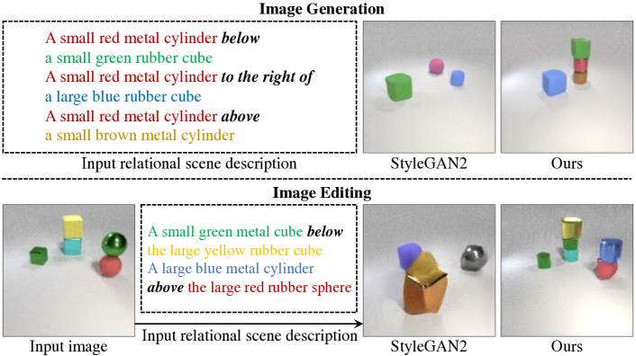
Figure 1: Our model can generate and edit images with multiple composed relations. Top: Image generation results based on relational scene descriptions. Bottom: Image editing results based on relational scene descriptions.

2 Related Work

Language Guided Scene Generation.

A large body of work has explored scene generation utilizing text descriptions [35, 40, 14, 31, 41, 39, 48, 49, 21, 18, 37, 47]. In contrast to our work, prior work [39, 48, 49, 18] have focused on generating images given only a limited number of relation descriptions. Recently, [37] shows compelling results on utilizing text to generate images, but also explicitly state that relational generation was a weakness of the model. In this work, we seek to tackle how we may generate images given an underlying relational description.

Visual Relation Understanding.

To understand visual relations in a scene, many works applied neural networks to graphs [21, 3, 38, 33, 29, 30, 15, 6, 16, 1, 19, 2]. Raposo et al. [38] proposed Relation Network (RN) to explicitly compute relations from static input scenes while we implicitly encode relational information to generate and edit images based on given relations and objects. Johnson et al. [21] proposed to condition image generation on relations by utilizing scene graphs which were further explored in [45, 32, 30, 16, 1, 15, 19]. However, these approaches require excessive supervisions, such as bounding boxes, segmentation masks, etc., to infer and generate the underlying relations in an image. Such a setting restricts the possible combinations of individual relations in a scene. In our work, we present a method that enables us to generate images given only a relational scene description.

Energy Based Models.

Our work is related to existing work on energy-based models [23, 43, 7, 46, 34, 13, 9, 11, 5]. Most similar to our work is that of [8], which proposes a framework of utilizing EBMs to compose several object descriptions together. In contrast, in this work, we study the problem of how we may compose relational descriptions together, an important and challenging task for existing text description understanding systems.

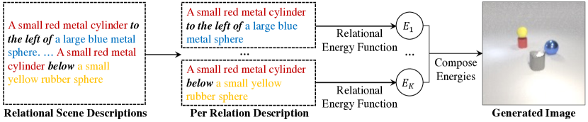
Figure 2: Overview of our pipeline for understanding a relational scene description. A relational scene description is split into a set of underlying relation descriptions. Individual relation descriptions are represented as EBMs which are subsequently composed together to generate an image.

3 Method

Given a training dataset $\mathcal{C}=\{{\bm{x}}_{i},R_{i}\}_{i=1}^{N}$ with $N$ distinct images ${\bm{x}}_{i}\in\mathbb{R}^{D}$ and associated relational descriptions $R_{i}$, we aim at learning the underlying probability distribution $p_{\theta}({\bm{x}}|R)$ — the probability distributions of an image given a corresponding relational description. To represent $p_{\theta}({\bm{x}}|R)$, we split a relational description $R$ into $K$ separate relations $\{r_{1}\cdots,r_{K}\}$ and model each component relation separately using a probability distribution $p_{\theta}({\bm{x}}|r_{k})$ which is represented as an Energy-Based Model. Our overall scene probability distribution is then modeled by a composition of individual probability distributions for each relation description $p_{\theta}({\bm{x}}|R)\propto\prod_{k}p_{\theta}({\bm{x}}|r_{k})$.

In this section, we give an overview of our approach towards factorizing and representing a relational scene description. We first provide a background overview of Energy-Based Models (EBMs) in Section 3.1. We then describe how we may parameterize individual relational probability distributions with EBMs in Section 3.2. We further describe how we compose relational probability distributions to model a relational scene description in Section 3.3. Finally, we illustrate downstream applications of our relational scene understanding model in Section 3.4.

3.1 Energy-Based Models

We model each relational probability distribution utilizing an Energy-Based Model (EBM) [27, 7]. EBMs are a class of unnormalized probability models, which parameterize a probability distribution $p_{\theta}({\bm{x}})$ utilizing a learned energy function $E_{\theta}(\bf x)$:

$$p_{\theta}({\bf x})\propto e^{-E_{\theta}({\bf x})}.$$ (1)

EBMs are typically trained utilizing contrastive divergence [17], where energies of training data-points are decreased and energies of sampled data points from $p_{\theta}({\bm{x}})$ are increased. We adopt the training code and models from [9] to train our EBMs. To generate samples from an EBM $p_{\theta}({\bm{x}})$, we utilize MCMC sampling on the underlying distribution, and Langevin dynamics, which refines a data sample iteratively from a random noise:

$$\tilde{\bf x}^{m}=\tilde{\bf x}^{m-1}-\frac{\lambda}{2}\nabla_{{\bf x}}E_{\theta}(\tilde{\bf x}^{m-1})+\omega^{m},\ \omega^{m}\sim\mathcal{N}(0,\sigma)$$ (2)

where $m$ refers to the iteration and $\lambda$ is the step size, utilizing the gradient of the energy function with respect to the input sample $\nabla_{{\bf x}}E_{\theta}$, and $\omega^{m}$ is sampled from a Gaussian noise. EBMs enable us to naturally compose separate probability distributions together [8]. In particular, given a set of independent marginal distributions $\{p_{\theta}^{i}({\bm{x}})\}$, the joint probability distribution is represented as:

$$\prod\limits_{i}p_{\theta}^{i}({{\bm{x}}})\propto e^{-\sum_{i}E_{\theta}^{i}({{\bm{x}}})},$$ (3)

where we utilize Langevin dynamics to sample from the resultant joint probability distribution.

3.2 Learning Relational Energy Functions

Given a scene relation $r_{i}$, described using a set of words $\{w_{i}^{1},\ldots w_{i}^{n}\}$, we seek to learn a conditional EBM to model the underlying probability distribution $p_{\theta}({\bm{x}}|r_{i})$:

$$p_{\theta}({\bm{x}};r_{i})\propto e^{-E^{i}_{\theta}({\bm{x}}|\text{Enc}(r_{i}))},$$ (4)

where $p_{\theta}({\bm{x}}|r_{i})$ represents the probability distribution over images given relation $r_{i}$ and $\text{Enc}(r_{i})$ denotes a text encoder for relation $r_{i}$.

The most straightforward manner to encode relational scene descriptions is to encode the entire sentence using an existing text encoder, such as CLIP [36]. However, we find that such an approach cannot capture scene relations as shown in Supplement Section A. An issue with such an approach is that the sentence encoder loses or masks the information captured by the relation tokens in $r_{i}$.

To enforce that the underlying relation tokens in $r_{i}$ is effectively encoded, we instead propose to decompose the relation $r_{i}$ into a relation triplet $(r^{\prime}_{i},o_{i}^{1},o_{i}^{2})$, where $r_{i}^{\prime}$ is the relation token, e.g. “below”, “to the right of”, $o_{i}^{1}$ is the description of the first object, and $o_{i}^{2}$ is the description of the second object appeared in $r_{i}$. Each separate entry in the relation triplet is then separately embedded.

Such an encoding scheme encourages the models to encode underlying objects and relations in a scene, enabling us to effectively model the relational distribution. We explored two separate approaches to embed the underlying object descriptions into our relational energy function.

CLIP Embedding.

One approach we consider is to directly utilize CLIP to obtain the embedding of an object description. Such an approach may potentially enable us to generalize relations in a zero-shot manner to new objects by utilizing CLIP’s underlying embedding of the object, but may also hurt learning if the underlying object embedding does not distinctly separate two object descriptions.

Random Initialization.

Alternatively, we may encode an object description using a learned embedding layer that is trained from scratch. In this approach, we extract a scene embedding by concatenating the learned embeddings of color, shape, material, and size of any two objects, $o_{i}^{1},o_{i}^{2}$, and their relation $r_{i}$.

3.3 Representing Relational Scene Descriptions

Given an underlying scene description $R$, we represent the underlying probability distribution $p({\bm{x}}|R)$ by factorizing it as a product of probabilities over the the underlying relations $r_{k}$ inside $R$.

Given the separate relational energy functions learned in Section 3.2, this probability $p({\bm{x}}|R)$ is proportional to

$$p({\bm{x}}|R)=e^{-E^{k}_{\theta}({\bm{x}}|R)}\propto\prod_{k}p({\bm{x}}|r_{k})=e^{-\sum\limits_{k}E^{k}_{\theta}({\bm{x}}|\text{Enc}(r_{k}))},$$ (5)

which is a new EBM with underlying energy function $E_{\theta}({\bm{x}}|R)=\sum\limits_{k}E^{k}_{\theta}({\bm{x}}|\text{Enc}(r_{k}))$. The overview of the proposed method is shown in Figure 2, where $E_{1},\cdots,E_{K}$ correspond to the $K$ individual relational energy functions $E^{k}_{\theta}{({\bm{x}}|\text{Enc}(r_{k}))}$.

3.4 Downstream Applications

By learning the probability distribution $p({\bm{x}}|R)$ with corresponding EBM $E_{\theta}({\bm{x}}|R)$, our model can be applied to solve many downstream applications, such as image generation, editing, and classification, which we detail below and validate in the experiment section.

Image Generation.

We generate images from a relational scene description $R$ by sampling from the probability distribution $p({\bm{x}}|R)$ using Langevin sampling on the energy function $E_{\theta}({\bm{x}}|R)$ from random noise.

Image Editing.

To edit an image ${\bm{x}}^{\prime}$, we utilize the same probability distribution $p({\bm{x}}|R)$ and Langevin sampling on the energy function $E_{\theta}({\bm{x}}|R)$ but initialize sampling from the image we wish to edit ${\bm{x}}^{\prime}$ instead of random noise.

Relational Scene Understanding.

We may further utilize the energy function $E_{\theta}({\bm{x}}|R)$ as a tool for relational scene understanding by noting that $p({\bm{x}}|R)\propto e^{-E_{\theta}({\bm{x}}|R)}$. The output values of the energy function can be used as a matching score of the generated/edited image and the given scene relational scene description $R$.

Table 1: Evaluation of the accuracy of object relations in the generated images or edited images on the CLEVR and iGibson datasets. We compare our method with baselines on three test sets, i.e. 1R, 2R, and 3R (see text).

Dataset	Model	Image Generation (%)			Image Editing (%)
		1R Acc	2R Acc	3R Acc	1R Acc	2R Acc	3R Acc
CLEVR	StyleGAN2	10.68	2.46	0.54	10.04	2.10	0.46
	StyleGAN2 (CLIP)	65.98	9.56	1.78	-	-	-
	Ours (CLIP)	94.79	48.42	18.00	95.56	52.78	16.32
	Ours (Learned Embed)	97.79	69.55	37.60	97.52	65.88	32.38
iGibson	StyleGAN2	12.46	2.24	0.60	11.04	2.18	0.84
	StyleGAN2 (CLIP)	49.20	17.06	5.10	-	-	-
	Ours (CLIP)	74.02	43.03	19.59	78.12	32.84	12.66
	Ours (Learned Embed)	78.27	45.03	19.39	84.16	44.10	20.76

4 Experiment

We conduct empirical studies to answer the following questions: (1) Can we learn relational models that can generate and edit complex multi-object scenes when given relational scene descriptions with multiple composed scene relations? (2) Can we use our model to generalize to scenes that are never seen in training? (3) Can we understand the set of relations in a scene and infer semantically equivalent descriptions?

To answer these questions, we evaluate the proposed method and baselines on image generation, image editing, and image classification on two main datasets, i.e. CLEVR [20] and iGibson [42]. We also test the image generation performance of the proposed model and baselines on a real-world dataset i.e. Blocks [28].

4.1 Datasets

CLEVR. We use $50,000$ pairs of images and relational scene descriptions for training. Each image contains $1\sim 5$ objects and each object consists of five different attributes, including color, shape, material, size, and its spatial relation to another object in the same image. There are $9$ types of colors, $4$ types of shapes, $3$ types of materials, $3$ types of sizes, and $6$ types of relations.

iGibson. On the iGibson dataset, we use 30,000 pairs of images and relational scene descriptions for training. Each image contains $1\sim 3$ objects and each object consists of the same five different types of attributes as the CLEVR dataset. There are $6$ types of colors, $5$ types of shapes, $4$ types of materials, $2$ types of sizes, and $4$ types of relations. The objects are randomly placed in the scenes.

Blocks. On the real-world Blocks dataset, a number of 3,000 pairs of images and relational scene descriptions are used for training. Each image contains $1\sim 4$ objects and each object differs in color. We only consider the “above” and “below” relations as objects are placed vertically in the form of towers.

In the training set, each image’s relational scene description only contains one scene relation and objects are randomly placed in the scene. We generated three test subsets that contain relational scene descriptions with a different number of scene relations to test the generation ability of the proposed methods and baselines. The 1R test subset is similar to the training set where each relational scene description contains one scene relation. The 2R and 3R test subsets have two and three scene relations in each relational scene description, respectively. Each test set has $5,000$ images with corresponding relational scene descriptions.

4.2 Baselines

We compare our method with two baseline approaches. The first baseline is StyleGAN2 [22], one of the state-of-the-art methods for unconditional image generation. To enable StyleGAN2 to generate images and edit images based on relational scene descriptions, we train a ResNet-18 classifier on top of it to predict the object attributes and their relations. Recently, CLIP [36] has achieved a substantial improvement on the text-image retrieval task by learning good text-image feature embeddings on large-scale datasets. Thus we design another baseline, StyleGAN2+CLIP, that combines the capabilities of both approaches. To do this, we encode relational scene descriptions into text embeddings using CLIP and condition StyleGAN2 on the embeddings to generate images. Please see Supplement Section E for more details of baselines.

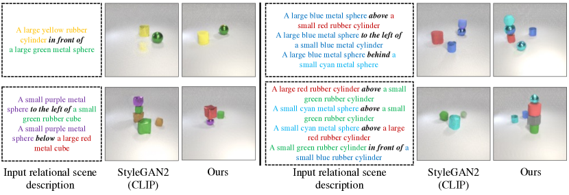
Figure 3: Image generation results on the CLEVR dataset. Image are generated based on 1 $\sim$ 4 relational descriptions. Note that the models are trained on a single relational description and the composed scene relations (2, 3, and 4 relational descriptions) are outside the training distribution.

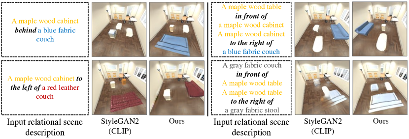
Figure 4: Image generation results on the iGibson dataset. Images are generated based on 1 $\sim$ 2 relational descriptions. Note that the two composed scene relations are outside the training distribution.

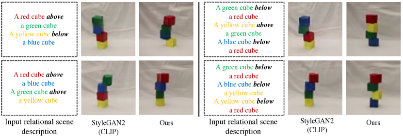
Figure 5: Image generation results on the Blocks dataset. Image are generated based the relational scene description. Note that the models are trained on a single relational scene description and the composed scene relations are outside the training distribution.

4.3 Image Generation Results

Given a relational scene description, e.g. “a blue cube on top of a red sphere”, we aim to generate images that contain corresponding objects and their relations as described in the given descriptions.

Quantitative comparisons. To evaluate the quality of generated images, we train a binary classifier to predict whether the generated image contains objects and their relations described in the given relational scene description.

Given a pair of an image and a relational scene description, we first feed the image to several convolutional layers to generate an image feature and then send the relational scene description to an embedding layer followed by several fully connected layers to generate a relational scene feature. The image feature and relational scene feature are combined and then passed through several fully connected and finally a sigmoid function to predict whether the given image matches the relational scene description. The binary classifier is trained on real images from the training dataset. We train a classifier on each dataset and observe classification accuracy on real images to be close to $100\%$, indicating that the classifier is effective. During testing, we generate an image based on a relational scene description and send the generated image and the relational scene description to the classifier for prediction. For a fair comparison, we use the same classifier to evaluate images generated by all the approaches on each dataset.

The “Image Generation” column in Table 1 shows the classification results of different approaches on the CLEVR and iGibson datasets. On each dataset, we test each method on three test subsets, i.e. 1R, 2R, 3R, and report their binary classification accuracies. Both variants of our proposed approach outperform StyleGAN2 and StyleGAN2 (CLIP), indicating that our method can generate images that contain the objects and their relations described in the relational scene descriptions. We find that our approach using the learned embedding, i.e. Ours (Learned Embed), achieves better performances on the CLEVR and iGibson datasets than the other variant using the CLIP embedding, i.e. Ours (CLIP).

StyleGAN2 and StyleGAN2 (CLIP) can perform well on the 1R test subset. This is an easier test subset because the models are trained on images with a single scene relation and the models generate images based on a single relational scene description during testing as well. The 2R and 3R are more challenging test subsets because the models need to generate images conditioned on relational scene descriptions of multiple scene relations. Our models outperform the baselines by a large margin, indicating the proposed approach has a better generalization ability and can compose multiple relations that are never seen during training.

Human evaluation results. To further evaluate the performance of the proposed method on image generation, we conduct a user study to ask humans to evaluate whether the generated images match the given input scene description. We compare the correctness of the object relations in the generated images and the input language of our proposed model, i.e. “Ours (Learned Embed)”, and “StyleGAN2 (CLIP)”. Given a language description, we generate an image using “Ours (Learned Embed)” and “StyleGAN2 (CLIP)”. We shuffle these two generated images and ask the workers to tell which image has better quality and the object relations match the input language description. We tested 300 examples in total, including 100 examples with 1 sentence relational description (1R), 100 examples with 2 sentence relational descriptions (2R), and 100 examples with 3 sentence relational descriptions (3R). There are 32 workers involved in this human experiment.

The workers think that there are 87%, 86%, and 91% of generated examples that “Ours (Learned Embed)” is better than “StyleGAN2 (CLIP)” for 1R, 2R, and 3R respectively. The human experiment shows that our proposed method is better than “StyleGAN2 (CLIP)”. The conclusion is coherent with our binary classification evaluation results.

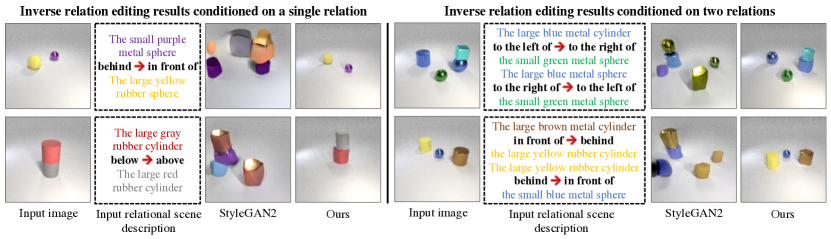
Figure 6: Image editing results on the CLEVR dataset. Left: image editing results based on a single relational scene description. Right: image editing results based on two composed relational scene descriptions. Note that the composed scene relations in the right part are outside the training distribution and our approach can still edit the images accurately.

Qualitative comparisons. The image generation results on CLEVR, iGibson and Block scenes are shown in Figure 3, 4, and 5, respectively. We show examples of generated images conditioned on relational scene descriptions of different number of scene relations. Our method generates images that are consistent with the relational scene descriptions. Note that both the proposed method and the baselines are trained on images that only contain a relational scene description of a single scene relation describing the visual relationship between two objects in each image. We find that our approach can still generalize well when composing more visual relations. Taking the upper right figure in Figure 3 as an example, a relational scene description of multiple scene relations, i.e. “A large blue metal sphere above a small red rubber cylinder. A large blue metal sphere to the left of a small blue metal cylinder $\cdots$”, is never seen during training. “StyleGAN2 (CLIP)” generates wrong objects and scene relations that are different from the scene descriptions. In contrast, our method has the ability to generalize to novel relational scenes.

4.4 Image Editing Results

Given an input image, we aim to edit this image based on relational scene descriptions, such as “put a red cube in front of the blue cylinder”.

Quantitative comparisons. Similar to the image generation, we use a classifier to predict whether the image after editing contains the objects and their relations described in the relational scene description. For the evaluation on each dataset, we use the same classifier for both image generation and image editing.

The “Image Editing” column in Table 1 shows the classification results of different approaches on the CLEVR and iGibson datasets. Both variants of our proposed approach, i.e. “Ours (CLIP)” and “Ours (Learned Embed)” outperform the baselines, i.e. “StyleGAN2” and “StyleGAN2 (CLIP)”, substantially. The good performance of our approach on the 2R and 3R test subsets shows that the proposed method has a good generalization ability to relational scene descriptions that are outside the training distribution. The images after editing based on relational scene descriptions can incorporate the described objects and their relations accurately.

Qualitative comparisons. We show image editing examples in Figure 6. The left part is image editing results conditioned on a single scene relation while the right part is conditioned on two scene relations. We show examples that edit images by inverting individual spatial relations between given two objects. Taking the first image in Figure 6 as an example, “the small purple metal sphere” is behind “the large yellow rubber sphere”, after editing, our model can successfully put “the small purple metal sphere” in front of “the large yellow rubber sphere”. Even for relational scene descriptions of two scene relations that are never seen during training, our model can edit images so that the selected objects are placed correctly.

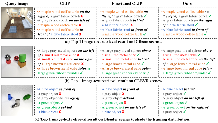
Figure 7: Image-to-text retrieval results. We compare the proposed approach with the pretrained CLIP and fine-tuned CLIP and show their top-1 retrieved relation description based on the given image query.

4.5 Relational Understanding

We hypothesize the good generation performance of our proposed approach is due to our system’s understanding of relations and ability to distinguish between different relational scene descriptions. In this section, we evaluate the relational understanding ability of our proposed method and baselines by comparing their image-to-text retrieval and semantic equivalence results.

Image-to-text retrieval. In Figure 7, we evaluate whether our proposed model can understand different relational scene descriptions by image-to-text retrieval. We create a test set that contains $240$ pairs of images and relational scene descriptions. Given a query image, we compute the similarity of this image and each relational scene description in the gallery set. The top 1 retrieved relational scene description is shown in Figure 7. We compare our method with two baselines. We use the pre-trained CLIP model and test it on our dataset directly. “Fine-tuned CLIP” means the CLIP model is fine-tuned on our dataset. Even though CLIP has shown good performance on the general image-text retrieval task, we find that it cannot understand spatial relations well, while EBMs can retrieve all the ground truth descriptions.

Table 2: Quantitative evaluation of semantic equivalence on the CLEVR dataset.

Model	Semantic Equivalence (%)
	1R Acc	2R Acc	3R Acc
Classifier	52.82	27.76	14.92
CLIP	37.02	14.40	5.52
CLIP (Fine-tuned)	60.02	35.38	20.9
Ours (CLIP)	70.68	50.48	38.06
Ours (Learned Emb)	74.76	57.76	44.86

We also find that our approach generalizes across datasets. In the bottom row of Figure 7, we conduct an additional image-to-text retrieval experiment on the Blender [4] scenes that are never seen during training. Our approach can still find the correct relational scene description for the query image.

Can we understand semantically equivalent relational scene descriptions? Given two relational scene descriptions describing the same image but in different ways, can our approach understand that the descriptions are semantically similar or equivalent? To evaluate this, we create a test subset that contains $5,000$ images and each image has $3$ different relational scene descriptions. There are two relational scene descriptions that match the image but describe the image in different ways, such as “a cabinet in front of a couch” and “a couch behind a cabinet”. There is one further description that does not match the image. The relative score difference between the two ground truth relational scene descriptions should be smaller than the difference between one ground truth relational scene description and one wrong relational scene description.

We compare our approach with three baselines. For each model, given an image, if the difference between two semantically equivalent relational scene description is smaller than the difference between the semantically different ones, we will classify it as correct. We compute the percentage of correct predictions and show the results in Table 2. Our proposed method outperforms the baselines substantially, indicating that our EBMs can distinguish semantically equivalent relational scene descriptions and semantically nonequivalent relational scene descriptions. In Figure 8, We further show two examples generated by our approach on the iGibson and CLEVR datasets. The energy difference between the semantically equivalent relational scene description is smaller than the mismatching pairs.

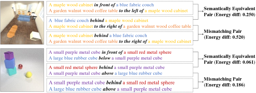
Figure 8: Examples of semantic equivalence on CLEVR and iGibson scenes. Given an input image, our approach is able to recognize whether the relational scene descriptions are semantically equivalent or not.

4.6 Zero-shot Generalization Across Datasets

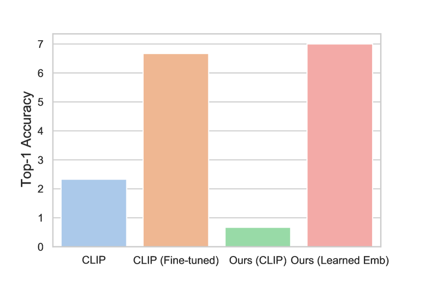
Figure 9: Zero-shot generalization on Blender scenes. Our approach with learned embedding outperforms other methods on image-to-text retrieval.

We find that our method can generalize across datasets as shown in the third example in Figure 7. To quantitatively evaluate the generalization ability across datasets of the proposed method, we test the image-to-text retrieval accuracy on the Blender dataset. We render a new Blender dataset using objects including boots, toys, and trucks. Note that our model and baselines are trained on CLEVR and have never seen the Blender scenes during training.

We generate a Blender test set that contains $300$ pairs of images and relational scene descriptions. For each image, we do text retrieval on the $300$ relational scene descriptions. The top 1 accuracy is shown in Figure 9. We compare our approaches with two baselines, i.e. CLIP and CLIP fine-tuned on the CLEVR dataset. We find the CLIP model and our approach using the CLIP embedding perform badly on the Blender dataset. This is because CLIP is not good at modeling relational scene description, as we have shown in Section 4.5. Our approach using the learned embedding outperforms other methods, indicating that our EBMs with a good embedding feature can generalize well even on unseen datasets, such as Blender.

5 Conclusion

In this paper, we demonstrate the potential usage for our model on compositional image generation, editing, and even generalization on unseen datasets given only relational scene descriptions. Our results provide evidence that EBMs are a useful class of models to study relational understanding.

One limitation of the current approach is that the evaluated datasets are simpler compared to the complex relational descriptions used in the real world. A good direction for future work would be to study how these models scale to complex datasets found in the real world. One particular interest could be measuring the zero-shot generalization capabilities of the proposed model.

Our system, as with all systems based on neural networks, is susceptible to dataset biases. The learned relations will exhibit biases if the training datasets are biased. We must take balanced and fair datasets if we develop our model to solve real-world problems, as otherwise, it could inadvertently worsen existing societal prejudices and biases.

Acknowledgements. Shuang Li is supported by Raytheon BBN Technologies Corp. under the project Symbiant (reg. no. 030256-00001 90113) and Mitsubishi Electric Research Laboratory (MERL) under the project Generative Models For Annotated Video. Yilun Du is supported by NSF graduate research fellowship and in part by ONR MURI N00014-18-1-2846 and IBM Thomas J. Watson Research Center CW3031624.

Supplement

In this supplementary material, we first present qualitative and quantitative comparisons with additional baseline approaches in Section A. We then show the experiment results on the more complex real world datasets in Section B and additional dataset details in Section C. More details of our proposed approach and baselines are shown in Section D and Section E, respectively. We provide the model architecture details of various approaches and their implementation details in Section G and Section H, respectively. Finally, we show the psuedocode for our algorithm in Section I.

Appendix A Additional Results

Comparison with more baseline approaches.

We provide more results of additional baselines in Table 3. We use the same evaluation metrics as in Table 1 of the main paper. The details of baselines are described in Section E of this supplement. As shown in Table 3 of this supplement, our approach achieves the highest accuracy among all the methods for both image generation and image editing. In Table 3, as noted in the main paper, directly encoding a relational scene description such as “a large blue rubber cube to the left of a small red metal cube” utilizing CLIP to train an EBM (“EBM (CLIP) (Full Sentence)”) performs much worse than the proposed method “Ours (CLIP)” and “Ours (Learned Embed)”.

Additional evaluation metric.

In addition to comparing the binary classification accuracy of different methods as we used in Table 1 of the main paper, we provide an additional evaluation metric for image generation. We investigate the performance of utilizing the graph-based relational similarity metric proposed by [10] for image generation. A graph-based relational similarity score is used to test the correct placement of objects, without requiring the model to draw the objects exactly in the same locations as the ground truth. Such a metric can construct scene graphs for both the generated and ground truth images without telling the model to precisely draw objects at the exact locations. However, it heavily relies on the pre-trained object detector and localizer. The pre-trained object detector or localizer could generate false predictions on both real images and generated images, especially when the generated images are out of the training distribution.

As the evaluation metric used in [10] focuses more on the local matching while our binary classification focuses on the global matching, in this supplement, we further report the results for two baselines and our approach using the evaluation metric proposed by [10]. The image generation results on the CLEVR dataset are listed in Table 4. The conclusion obtained by using this new metric is coherent with using our binary classification metric (Table 1 of the main paper): our proposed method outperforms the baselines.

Table 3: Evaluation of the accuracy of object relations in the generated images or edited images on the CLEVR and iGibson datasets. We compare our method with baselines on three test sets, i.e. 1R, 2R, and 3R. In Table 1 of the main paper, we had two baselines, i.e. StyleGAN2 and StyleGAN2 (CLIP). Here we add another 3 baselines, i.e. Scene Graph GAN [21], EBM (CLIP) (Full Sentence), and StyleGAN2 (CLIP) (Multi-Relations), for comparison.

Dataset	Model	Image Generation (%)
		1R Acc	2R Acc	3R Acc
CLEVR	StyleGAN2	10.68	2.46	0.54
	StyleGAN2 (CLIP)	65.98	9.56	1.78
	StyleGAN2 (CLIP) (Multi-Relations)	66.62	9.60	1.68
	Scene Graph GAN	83.72	14.18	4.48
	EBM (CLIP) (Full Sentence)	4.75	0.24	0.00
	Ours (CLIP)	94.79	48.42	18.00
	Ours (Learned Embed)	97.79	69.55	37.60
iGibson	StyleGAN2	12.46	2.24	0.60
	StyleGAN2 (CLIP)	49.20	17.06	5.10
	StyleGAN2 (CLIP) (Multi-Relations)	36.94	13.42	6.86
	Scene Graph GAN	54.64	0.02	0.00
	EBM (CLIP) (Full Sentence)	34.25	8.05	3.47
	Ours (CLIP)	74.02	43.04	19.59
	Ours (Learned Embed)	78.27	45.03	19.39

Table 4: Comparison of different methods on the CLEVR dataset. The accuracy of graph-based relational similarity proposed by [10] is reported.

Model	Relational Similarity (%)
	1R Acc	2R Acc	3R Acc
StyleGAN2	22.37	19.75	17.13
StyleGAN2 (CLIP)	37.50	28.62	28.75
Ours (Learned Emb)	50.77	36.87	42.50

Additional qualitative results.

We show more qualitative results of image generation in Figure 10 and Figure 11. Our approach can generate images with correct relations, and can even generalize to relational scene descriptions that are out of the training distribution.

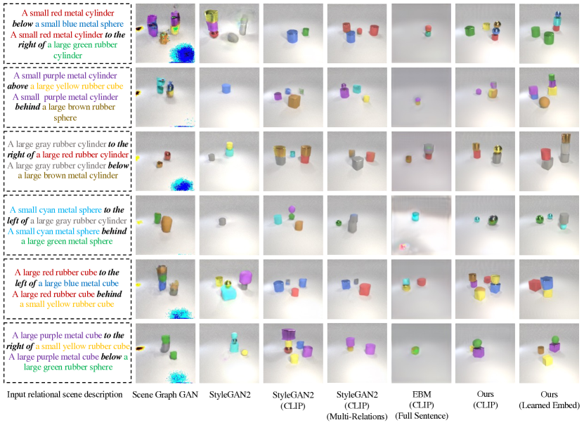
Figure 10: Image generation results on the CLEVR dataset. Image are generated based on 2 relational descriptions. Note that the models are trained on a single relational description and the two composed scene relations are outside the training distribution. Our approaches “Ours (CLIP)” and “Ours (Learned Embed)” are able to generate images accurately based on the input scene descriptions.

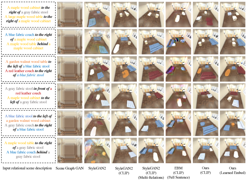
Figure 11: Image generation results on the iGibson dataset. Image are generated based on 2 relational descriptions. Note that the models are trained on a single relational description and the two composed scene relations are outside the training distribution. Our approaches “Ours (CLIP)” and “Ours (Learned Embed)” are able to generate images accurately based on the input scene descriptions.

Appendix B Image Generation Results on Real World Datasets

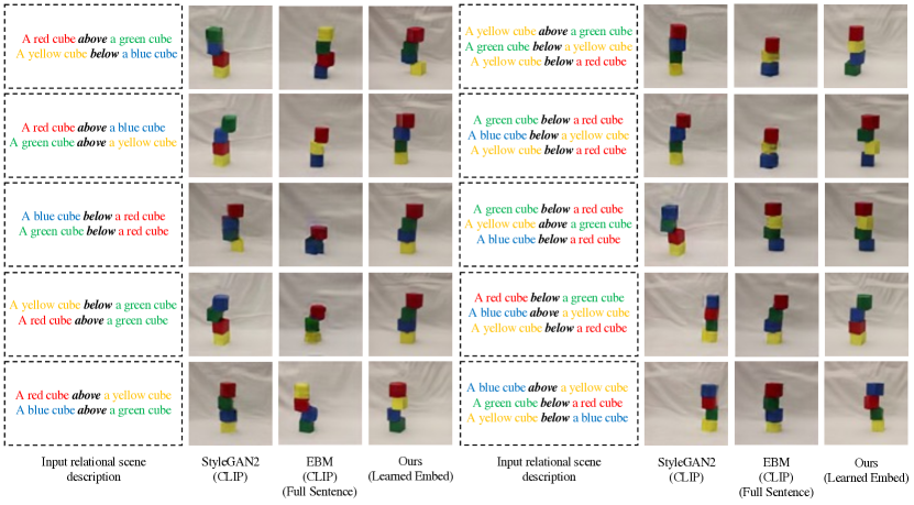
Figure 12: Image generation results on the Block dataset. Image are generated based on 2 or 3 relational descriptions. Note that the models are trained on a single relational description and the composed scene relations (2 and 3 relational descriptions) are outside the training distribution. Our approach “Ours (Learned Embed)” is able to generate images accurately based on the input scene descriptions.

In terms of image generation on real scenes, we train and evaluate our model on two real-world datasets, the Blocks dataset [28] and the Visual Genome dataset [25].

The Blocks dataset is from [28] and we train our model using the object relations, e.g. “above” and “below”. We show the images generated conditioned on two relational descriptions and three relational descriptions in Figure 12.

For the Visual Genome dataset [25], we train our models on a subset that consists of common objects and relations for computational efficiency. As shown in Figure 13, we find that the CLIP text encoder performs better, as it has seen large-scale image-text pairs that cover a wide range of relations, attributes and objects.

Our approach is able to generate images (objects and their relations) matching the given language descriptions on the real-world Blocks dataset and the Visual Genome dataset. The quality of generated images on the Blocks dataset is great. However, the quality of results on the Visual Genome dataset is a bit worse. We believe that the generation quality could be further improved.

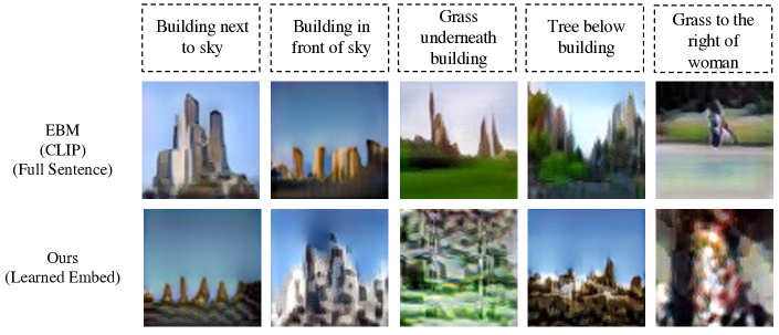
Figure 13: Image generation results on the Visual Genome dataset. “EBM (CLIP) (Full Sentence)” performs better than our approach “Ours (Learned Emb)” on generating more complex natural images because pretrained CLIP text encoder has seen large-scale image-text pairs that cover a wide range of relations and objects.

Appendix C Datasets Details

CLEVR. On the CLEVR dataset, each image contains $1\sim 5$ objects and each object consists of five different attributes, including color, shape, material, size, and its relation to another object in the same image. There are $9$ types of colors, $4$ types of shapes, $3$ types of materials, $3$ types of sizes, and $6$ types of relations. The objects are randomly placed in the scenes.

iGibson. On the iGibson dataset, each image contains $1\sim 3$ objects and each object consists of the same five different types of attributes as the CLEVR dataset. There are $6$ types of colors, $5$ types of shapes, $4$ types of materials, $2$ types of sizes, and $4$ types of relations. The objects are randomly placed in the scenes.

Blocks. On the real-world Blocks dataset, each image contains $1\sim 4$ cubes and each cube only differs in color. Objects in the images are placed vertically in the form of towers.

There are 50,000, 30,000 and 3,000 training images on the CLEVR, iGibson and Blocks datasets, respectively, and 5,000 testing images on both the CLEVR and iGibson datasets. We test the zero-shot generalization across datasets using the blender data. There are three types of objects, including trucks, toys, and boots. We generated 5,000 testing images with each image contains $1\sim 3$ objects for the Blocks dataset. There is no overlap between the training and testing data on each dataset.

Appendix D Details of Our Approaches

Ours (CLIP).

In our EBM setting, we use the pre-trained CLIP model to encode objects and a learned embedding layer to encode their relations. Taking the scene description of “a large blue rubber cube to the left of a small red metal cube” as an example, we use the pre-trained CLIP model to encode the two objects seperately, i.e. $o^{1}$ for “a large blue rubber cube” and $o^{2}$ for “a small red metal cube”. We then use an embedding layer to encode their relation, i.e. $r^{\prime}$ for “to the left”. The features of the first and second objects and their relations are concatenated and used as the feature of the relational scene description which is further send to the relational energy functions $E_{\theta}$ for image generation or image editting.

Ours (Learned Embed).

Different from “Ours (CLIP)”, “Ours (Learned Embed)” uses the learned embedding layers for both objects and their relations. To encode an object, we use 6 different embedding layers to learn its color, size, material, shape, relation and position, seperately. The embedded features of objects and their relations are concatenated and used as the feature of the relational scene description which is further sent to the relational energy functions $E_{\theta}$ for image generation or image editting.

Appendix E Details of Baselines

StyleGAN2.

In Section 4.2 of the main paper, we used the unconditional StyleGAN2 [22] as one of the baselines. We train the unconditional StyleGAN2 and the ResNet-18 classifier separately on each dataset. For training, we use the default setting provided by [22]. To generate an image with respect to a particular relation, we optimize the underlying latent code to minimize the loss from the classifier.

StyleGAN2 (CLIP).

StyleGAN2 (CLIP) is the same as StyleGAN2 except that StyleGAN2 (CLIP) uses the text encoder of the CLIP model [36] to encode relational scene descriptions. We follow the same configuration as the StyleGAN2 to train StyleGAN2 (CLIP).

StyleGAN2 (CLIP) (Multi-Relations).

StyleGAN2 (CLIP) (Multi-Relations) has the same model architecture as StyleGAN2 (CLIP) but is trained with more scene relations. In StyleGAN2 (CLIP), we only use a single scene relation during training while StyleGAN2 (CLIP) (Multi-Relations) uses $1\sim 3$ scene relations.

Scene Graph GAN.

We apply the models from [21] and utilize the extracted scene graphs as input to train a conditional StyleGAN2. As there is no object bounding boxes available in our setting, we set the input bounding box to be the whole image frame and our input scene graphs only consist of two objects and their relation.

EBM (CLIP) (Full Sentence).

In this setting, we use the text encoder of CLIP to encode every word in the relational scene descriptions. Such a holistic encoder has a bad performance as shown in Table 3, Figure 10, Figure 11 and Figure 12.

Appendix F Inference Details

In this section, we introduce the inference details of image generation and image editing using our proposed method.

Image Generation.

Given an input scene description and the random noise map, we run 10 alternating series of data augmentation and Langevin sampling to get an intermediate result. Then we run the Langevin sampling 80 steps to generate the final image.

Image Editing.

After splitting a relational scene description into corresponding input labels, we simply run Langevin sampling on the input image with 80 steps to generate the final image. The step size used in image editing applies the same rule as we used in image generation.

Appendix G Model Architecture Details

Table 5: We use the multi-scale model architecture to compute energies as in [9].

3x3 Conv2d 128
CondResBlock 128
CondResBlock Down 128
CondResBlock 128
CondResBlock Down 256
Self-Attention 256
CondResBlock 256
CondResBlock Down 256
CondResBlock 512
CondResBlock Down 512
Global Mean Pooling
Dense $\to$ 1

3x3 Conv2d 128
CondResBlock 128
CondResBlock Down 128
CondResBlock 128
CondResBlock Down 128
Self-Attention 256
CondResBlock 256
CondResBlock Down 256
Global Mean Pooling
Dense $\to$ 1

3x3 Conv2d 128
CondResBlock 128
CondResBlock Down 128
Self-Attention 128
CondResBlock 128
CondResBlock Down 128
Global Mean Pooling
Dense $\to$ 1

We follow the implementation of EBMs from [9] in our experiments. Similar to [9], we use the multi-scale model architecture to compute energies as shown in Table 5. Each model generates an energy value and the final energy $E_{\theta}({\mathbf{x}})$ is the sum of energies from all the models listed in Table 5. Given relational scene descriptions, we generate or edit images based on the final energy.

Appendix H Implementation Details

StyleGAN2.

It takes 2 days to train the StyleGAN2 model and 2 hours to train the classifier using a single Tesla 32GB GPU on each dataset. We use the Adam optimizer [24] with $\beta_{1}=0$, $\beta_{2}=0.99$, and $\epsilon=10^{-8}$ to train the model.

StyleGAN2 (CLIP).

For StyleGAN2 (CLIP) and StyleGAN2 (CLIP) (Multi-Relations), it takes around 2 days to train each of them on each dataset using a single Tesla 32GB GPU. We use the Adam optimizer [24] with $\beta_{1}=0$, $\beta_{2}=0.99$, and $\epsilon=10^{-8}$ to train them.

Scene Graph GAN.

We train the model on each dataset with the default training configuration provided in the codebase from [21] for 2 days using a single Tesla 32GB GPU. We use the Adam optimizer [24] with $\beta_{1}=0.9$, $\beta_{2}=0.999$, and $\epsilon=10^{-4}$ to train the model.

EBMs (i.e., Ours (CLIP), Ours (Learned Embed), EBM (CLIP) (Full Sentence)).

In our experiments, we use the same setting to train models using EBMs, i.e., Ours (CLIP), Ours (Learned Embed), and EBM (CLIP) (Full Sentence), for fair comparison. We use the Adam optimizer [24] with learning rates of $10^{-4}$ and $2\times 10^{-4}$ on the CLEVR and iGibson datasets, respectively. For MCMC sampling, we use a step size of 300 on the CLEVR dataset, 750 on the iGibson dataset and 300 on the Blocks dataset. On each dataset, the model is trained for 3 days on a single Tesla 32GB GPU.

To generate images at test time, we initialize an image sample from random noise. We then iteratively apply data augmentation on the image sample followed by 20 steps of Langevin sampling. To generate the final image, we run 80 additional steps of Langevin sampling on the image sample.

To edit images at test time, we run 80 steps of Langevin sampling on the image to edit. The step size of Langevin sampling is inversely proportional to the number of scene relations, i.e. more scene relations leads to a lower Langevin sampling step size.

Appendix I Algorithms

We provide the algorithms of the proposed method, including training, image generation, image editing, and image-to-text retrieval, in Algorithm 1, 2, 3 and 4, respectively.

  Input: data dist $p_{D}({\bm{x}})$, relational scene descriptions $R_{D}({\bm{r}})$, step size $\lambda$, number of steps $K$, data augmentation $D(\cdot)$, stop gradient operator $\Omega(\cdot)$, EBM $E_{\theta}(\cdot)$, Encoder Enc$(\cdot)$

  $\mathcal{B}\leftarrow\varnothing$

  while not converged do

     ${\bm{x}}^{+}_{i}\sim p_{D}$

     $R_{i}\sim R_{D}$

     $\tilde{{\bm{x}}}^{0}_{i}\sim\mathcal{B}$ with 99% probability and $\mathcal{U}$ otherwise

     $X\sim\mathcal{B}$ for nearest neighbor entropy calculation

     $\triangleright$ Split a relational scene description into individual scene relations:

     $\{{\bm{r}}_{1},\dots\bm{r}_{m}\}\leftarrow R_{i}$

     $\triangleright$ Apply data augmentation to sample:

     $\tilde{{\bm{x}}}^{0}_{i}=D(\tilde{{\bm{x}}}^{0}_{i})$

     $\triangleright$ Generate sample using Langevin dynamics:

     for sample step $k=1$ to $K$ do

        $\tilde{{\bm{x}}}^{k-1}_{i}=\Omega(\tilde{{\bm{x}}}^{k-1}_{i})$

        $\tilde{{\bm{x}}}^{k}\leftarrow\tilde{{\bm{x}}}^{k-1}-\nabla_{\bm{x}}\sum_{j=1}^{m}E_{\theta}(\tilde{{\bm{x}}}^{k-1}\ |\ \text{Enc}({\bm{r}}_{j}))+\omega,\;\;\omega\sim\mathcal{N}(0,\sigma)$

     end for

     $\triangleright$ Generate two variants of ${\bm{x}}^{-}$ with and without gradient propagation:

     ${\bm{x}}^{-}_{i}=\Omega(\tilde{{\bm{x}}}^{k}_{i})$

     $\hat{{\bm{x}}}^{-}_{i}=\tilde{{\bm{x}}}^{k}_{i}$

     $\triangleright$ Optimize objective $\mathcal{L}_{\text{CD}}+\mathcal{L}_{\text{KL}}$ wrt $\theta$:

     $\mathcal{L}_{\text{CD}}=\frac{1}{N}\sum_{i}\sum_{j=1}^{m}(E_{\theta}({\bm{x}}^{+}_{i}\ |\ \text{Enc}({\bm{r}}_{j})-E_{\theta}({\bm{x}}^{-}_{i}\ |\ \text{Enc}({\bm{r}}_{j}))$

     $\mathcal{L}_{\text{KL}}=\sum_{j=1}^{m}E_{\Omega(\theta)}(\hat{{\bm{x}}}^{-}_{i}\ |\ \text{Enc}({\bm{r}}_{j}))-\log(NN(\hat{{\bm{x}}}^{-}_{i},X)$

     $\triangleright$ Optimize objective $\mathcal{L}_{\text{CD}}+\mathcal{L}_{\text{KL}}$ wrt $\theta$:

     $\Delta\theta\leftarrow\nabla_{\theta}(\mathcal{L}_{\text{CD}}+\mathcal{L}_{\text{KL}})$

     Update $\theta$ based on $\Delta\theta$ using Adam optimizer

     $\triangleright$ Update replay buffer $\mathcal{B}$

     $\mathcal{B}\leftarrow\mathcal{B}\cup\tilde{{\bm{x}}}_{i}^{-}$

  end while

Algorithm 1 Conditional EBM training algorithm

  Input: Relational scene description $R$, number of data augmentation applications $N$, step size $\lambda$, number of steps $K$, data augmentation $D(\cdot)$, EBM $E_{\theta}(\cdot)$, Encoder Enc$(\cdot)$

  $\tilde{{\bm{x}}}^{0}\sim\mathcal{U}$

  $\triangleright$ Split a relational scene description into individual scene relations:

  $\{{\bm{r}}_{1},\dots\bm{r}_{m}\}\leftarrow R$

  $\triangleright$ Generate samples through $N$ iterative steps of data augmentation/Langevin dynamics:

  for sample step $n=1$ to $N$ do

     $\triangleright$ Apply data augmentation to samples:

     $\tilde{{\bm{x}}}^{0}=D(\tilde{{\bm{x}}}^{0}_{i})$

     $\triangleright$ Run $K$ steps of Langevin dynamics:

     for sample step $k=1$ to $K$ do

        $\tilde{{\bm{x}}}^{k}\leftarrow\tilde{{\bm{x}}}^{k-1}-\sum_{i=1}^{n}\nabla_{\bm{x}}E_{\theta}(\tilde{{\bm{x}}}^{k-1}\ |\ \text{Enc}({\bm{r}}_{i}))+\omega,\;\;\omega\sim\mathcal{N}(0,\sigma)$

     end for

     $\triangleright$ Iteratively refine samples:

     $\tilde{{\bm{x}}}^{0}=\tilde{{\bm{x}}}^{k}$

  end for

  $\triangleright$ Final output:

  ${\bm{x}}=\tilde{{\bm{x}}}^{0}$

Algorithm 2 Image generation during testing

  Input: input image $\tilde{{\bm{x}}}^{0}$, relational scene description $R$, number of data augmentation applications $N$, step size $\lambda$, number of steps $K$, data augmentation $D(\cdot)$, EBM $E_{\theta}(\cdot)$ Encoder Enc$(\cdot)$

  $\triangleright$ Split a relational scene description into individual scene relations:

  $\{{\bm{r}}_{1},\dots\bm{r}_{m}\}\leftarrow R$

  $\triangleright$ Generate samples through $N$ iterative steps of data augmentation/Langevin dynamics:

  for sample step $n=1$ to $N$ do

     $\triangleright$ Apply data augmentation to samples:

     $\tilde{{\bm{x}}}^{0}=D(\tilde{{\bm{x}}}^{0}_{i})$

     $\triangleright$ Run $K$ steps of Langevin dynamics:

     for sample step $k=1$ to $K$ do

        $\tilde{{\bm{x}}}^{k}\leftarrow\tilde{{\bm{x}}}^{k-1}-\sum_{i=1}^{n}\nabla_{\bm{x}}E_{\theta}(\tilde{{\bm{x}}}^{k-1}\ |\ \text{Enc}({\bm{r}}_{i}))+\omega,\;\;\omega\sim\mathcal{N}(0,\sigma)$

     end for

     $\triangleright$ Iteratively refine samples:

     $\tilde{{\bm{x}}}^{0}=\tilde{{\bm{x}}}^{k}$

  end for

  $\triangleright$ Final output:

  ${\bm{x}}=\tilde{{\bm{x}}}^{0}$

Algorithm 3 Image editing during testing

  Input: input image ${\bm{x}}$, relational scene descriptions $\{R_{1},\dots,R_{n}\}$, EBM $E_{\theta}(\cdot)$, Encoder Enc$(\cdot)$, output energy list $\mathcal{O}$, caption prediction $\mathcal{C}$

  $\mathcal{O}\leftarrow[]$

  $\triangleright$ Generate image-caption matching energies iteratively

  for number of scene relations descriptions $i=1$ to $n$ do

     $\triangleright$ Split a relational scene description into individual scene relations:

     $\{{\bm{r}}_{1},\dots\bm{r}_{m}\}\leftarrow R_{i}$

     ${\bm{e}}_{i}=\sum_{j=1}^{m}E_{\theta}({\bm{x}}\ |\ \text{Enc}({\bm{r}}_{j}))$

     $\triangleright$ output energy list $\mathcal{O}$

     $\mathcal{O}.append({\bm{e}}_{i})$

  end for

  $\triangleright$ Final output:

  $\mathcal{C}=\operatorname*{arg\,min}\mathcal{O}$

Algorithm 4 Image-to-text retrieval during testing

References

- Ashual and Wolf [2019] Oron Ashual and Lior Wolf. Specifying object attributes and relations in interactive scene generation. In Proceedings of the IEEE/CVF International Conference on Computer Vision, pages 4561–4569, 2019.
- Bar et al. [2020] Amir Bar, Roei Herzig, Xiaolong Wang, Gal Chechik, Trevor Darrell, and Amir Globerson. Compositional video synthesis with action graphs. arXiv preprint arXiv:2006.15327, 2020.
- Battaglia et al. [2016] Peter W Battaglia, Razvan Pascanu, Matthew Lai, Danilo Rezende, and Koray Kavukcuoglu. Interaction networks for learning about objects, relations and physics. arXiv preprint arXiv:1612.00222, 2016.
- Community [2018] Blender Online Community. Blender - a 3D modelling and rendering package. Blender Foundation, Stichting Blender Foundation, Amsterdam, 2018. URL http://www.blender.org.
- Dai et al. [2020] Bo Dai, Zhen Liu, Hanjun Dai, Niao He, Arthur Gretton, Le Song, and Dale Schuurmans. Exponential family estimation via adversarial dynamics embedding, 2020.
- De Cao and TMGAN [2018] N De Cao and Kipf TMGAN. An implicit generative model for small molecular graphs. arxiv preprint 2018. arXiv preprint arXiv:1805.11973, 2018.
- Du and Mordatch [2019] Yilun Du and Igor Mordatch. Implicit generation and generalization in energy-based models. arXiv preprint arXiv:1903.08689, 2019.
- Du et al. [2020a] Yilun Du, Shuang Li, and Igor Mordatch. Compositional visual generation and inference with energy based models. arXiv preprint arXiv:2004.06030, 2020a.
- Du et al. [2020b] Yilun Du, Shuang Li, Joshua Tenenbaum, and Igor Mordatch. Improved contrastive divergence training of energy based models. arXiv preprint arXiv:2012.01316, 2020b.
- El-Nouby et al. [2018] Alaaeldin El-Nouby, Shikhar Sharma, Hannes Schulz, Devon Hjelm, Layla El Asri, Samira Ebrahimi Kahou, Yoshua Bengio, and Graham W Taylor. Keep drawing it: Iterative language-based image generation and editing. arXiv preprint arXiv:1811.09845, 2, 2018.
- Gao et al. [2020] Ruiqi Gao, Erik Nijkamp, Diederik P Kingma, Zhen Xu, Andrew M Dai, and Ying Nian Wu. Flow contrastive estimation of energy-based models. In Proceedings of the IEEE/CVF Conference on Computer Vision and Pattern Recognition, pages 7518–7528, 2020.
- Garrett et al. [2021] Caelan Reed Garrett, Rohan Chitnis, Rachel Holladay, Beomjoon Kim, Tom Silver, Leslie Pack Kaelbling, and Tomás Lozano-Pérez. Integrated task and motion planning. Annual review of control, robotics, and autonomous systems, 4:265–293, 2021.
- Grathwohl et al. [2019] Will Grathwohl, Kuan-Chieh Wang, Jörn-Henrik Jacobsen, David Duvenaud, Mohammad Norouzi, and Kevin Swersky. Your classifier is secretly an energy based model and you should treat it like one. arXiv preprint arXiv:1912.03263, 2019.
- Gregor et al. [2015] Karol Gregor, Ivo Danihelka, Alex Graves, Danilo Rezende, and Daan Wierstra. Draw: A recurrent neural network for image generation. In International Conference on Machine Learning, pages 1462–1471. PMLR, 2015.
- Gu et al. [2019] Jiuxiang Gu, Handong Zhao, Zhe Lin, Sheng Li, Jianfei Cai, and Mingyang Ling. Scene graph generation with external knowledge and image reconstruction. In Proceedings of the IEEE/CVF Conference on Computer Vision and Pattern Recognition, pages 1969–1978, 2019.
- Herzig et al. [2020] Roei Herzig, Amir Bar, Huijuan Xu, Gal Chechik, Trevor Darrell, and Amir Globerson. Learning canonical representations for scene graph to image generation. In European Conference on Computer Vision, pages 210–227. Springer, 2020.
- Hinton [2002] Geoffrey E. Hinton. Training products of experts by minimizing contrastive divergence. Neural Comput., 14(8):1771–1800, August 2002. ISSN 0899-7667. doi: 10.1162/089976602760128018. URL https://doi.org/10.1162/089976602760128018.
- Hong et al. [2018] Seunghoon Hong, Dingdong Yang, Jongwook Choi, and Honglak Lee. Inferring semantic layout for hierarchical text-to-image synthesis. In Proceedings of the IEEE Conference on Computer Vision and Pattern Recognition, pages 7986–7994, 2018.
- Hua et al. [2021] Tianyu Hua, Hongdong Zheng, Yalong Bai, Wei Zhang, X. Zhang, and Tao Mei. Exploiting relationship for complex-scene image generation. In AAAI, 2021.
- Johnson et al. [2017] Justin Johnson, Bharath Hariharan, Laurens Van Der Maaten, Li Fei-Fei, C Lawrence Zitnick, and Ross Girshick. Clevr: A diagnostic dataset for compositional language and elementary visual reasoning. In Proceedings of the IEEE conference on computer vision and pattern recognition, pages 2901–2910, 2017.
- Johnson et al. [2018] Justin Johnson, Agrim Gupta, and Li Fei-Fei. Image generation from scene graphs. 2018 IEEE/CVF Conference on Computer Vision and Pattern Recognition, pages 1219–1228, 2018.
- Karras et al. [2020] Tero Karras, M. Aittala, Janne Hellsten, S. Laine, J. Lehtinen, and Timo Aila. Training generative adversarial networks with limited data. ArXiv, abs/2006.06676, 2020.
- Kim and Bengio [2016] Taesup Kim and Yoshua Bengio. Deep directed generative models with energy-based probability estimation. ArXiv, abs/1606.03439, 2016.
- Kingma and Ba [2014] Diederik P Kingma and Jimmy Ba. Adam: A method for stochastic optimization. arXiv preprint arXiv:1412.6980, 2014.
- Krishna et al. [2017] Ranjay Krishna, Yuke Zhu, Oliver Groth, Justin Johnson, Kenji Hata, Joshua Kravitz, Stephanie Chen, Yannis Kalantidis, Li-Jia Li, David A Shamma, et al. Visual genome: Connecting language and vision using crowdsourced dense image annotations. International journal of computer vision, 123(1):32–73, 2017.
- Lake et al. [2015] B. Lake, R. Salakhutdinov, and J. Tenenbaum. Human-level concept learning through probabilistic program induction. Science, 350:1332 – 1338, 2015.
- LeCun et al. [2006] Yann LeCun, Sumit Chopra, Raia Hadsell, Marc’Aurelio Ranzato, and Fu-Jie Huang. A tutorial on energy-based learning. In G. Bakir, T. Hofman, B. Schölkopf, A. Smola, and B. Taskar, editors, Predicting Structured Data. MIT Press, 2006.
- Lerer et al. [2016] Adam Lerer, Sam Gross, and Rob Fergus. Learning physical intuition of block towers by example. In International conference on machine learning, pages 430–438. PMLR, 2016.
- Li et al. [2019a] Jianan Li, Jimei Yang, Aaron Hertzmann, Jianming Zhang, and Tingfa Xu. Layoutgan: Generating graphic layouts with wireframe discriminators. ArXiv, abs/1901.06767, 2019a.
- Li et al. [2019b] Yikang Li, Tao Ma, Yeqi Bai, Nan Duan, Sining Wei, and Xiaogang Wang. Pastegan: A semi-parametric method to generate image from scene graph. In NeurIPS, 2019b.
- Mansimov et al. [2015] Elman Mansimov, Emilio Parisotto, Jimmy Lei Ba, and Ruslan Salakhutdinov. Generating images from captions with attention. arXiv preprint arXiv:1511.02793, 2015.
- Mittal et al. [2019] Gaurav Mittal, Shubham Agrawal, Anuva Agarwal, Sushant Mehta, and T. Marwah. Interactive image generation using scene graphs. ArXiv, abs/1905.03743, 2019.
- Nauata et al. [2020] Nelson Nauata, Kai-Hung Chang, Chin-Yi Cheng, Greg Mori, and Yasutaka Furukawa. House-gan: Relational generative adversarial networks for graph-constrained house layout generation. In European Conference on Computer Vision, pages 162–177. Springer, 2020.
- Nijkamp et al. [2020] Erik Nijkamp, Mitch Hill, Tian Han, Song-Chun Zhu, and Y. Wu. On the anatomy of mcmc-based maximum likelihood learning of energy-based models. ArXiv, abs/1903.12370, 2020.
- Oord et al. [2016] Aaron van den Oord, Nal Kalchbrenner, Oriol Vinyals, Lasse Espeholt, Alex Graves, and Koray Kavukcuoglu. Conditional image generation with pixelcnn decoders. arXiv preprint arXiv:1606.05328, 2016.
- Radford et al. [2021] Alec Radford, Jong Wook Kim, Chris Hallacy, Aditya Ramesh, Gabriel Goh, Sandhini Agarwal, Girish Sastry, Amanda Askell, Pamela Mishkin, Jack Clark, et al. Learning transferable visual models from natural language supervision. arXiv preprint arXiv:2103.00020, 2021.
- Ramesh et al. [2021] Aditya Ramesh, Mikhail Pavlov, Gabriel Goh, Scott Gray, Chelsea Voss, Alec Radford, Mark Chen, and Ilya Sutskever. Zero-shot text-to-image generation. arXiv preprint arXiv:2102.12092, 2021.
- Raposo et al. [2017] David Raposo, Adam Santoro, David Barrett, Razvan Pascanu, Timothy Lillicrap, and Peter Battaglia. Discovering objects and their relations from entangled scene representations. arXiv preprint arXiv:1702.05068, 2017.
- Reed et al. [2016a] Scott Reed, Zeynep Akata, Xinchen Yan, Lajanugen Logeswaran, Bernt Schiele, and Honglak Lee. Generative adversarial text to image synthesis. In International Conference on Machine Learning, pages 1060–1069. PMLR, 2016a.
- Reed et al. [2017] Scott Reed, Aäron Oord, Nal Kalchbrenner, Sergio Gómez Colmenarejo, Ziyu Wang, Yutian Chen, Dan Belov, and Nando Freitas. Parallel multiscale autoregressive density estimation. In International Conference on Machine Learning, pages 2912–2921. PMLR, 2017.
- Reed et al. [2016b] Scott E Reed, Zeynep Akata, Santosh Mohan, Samuel Tenka, Bernt Schiele, and Honglak Lee. Learning what and where to draw. Advances in neural information processing systems, 29:217–225, 2016b.
- Shen et al. [2020] Bokui Shen, Fei Xia, Chengshu Li, Roberto Martín-Martín, Linxi Fan, Guanzhi Wang, Shyamal Buch, Claudia D’Arpino, Sanjana Srivastava, Lyne P Tchapmi, et al. igibson, a simulation environment for interactive tasks in large realistic scenes. arXiv preprint arXiv:2012.02924, 2020.
- Song and Ou [2018] Yunfu Song and Zhijian Ou. Learning neural random fields with inclusive auxiliary generators. arXiv preprint arXiv:1806.00271, 2018.
- Stilman and Kuffner [2005] Mike Stilman and James J Kuffner. Navigation among movable obstacles: Real-time reasoning in complex environments. International Journal of Humanoid Robotics, 2(04):479–503, 2005.
- Tripathi et al. [2019] Subarna Tripathi, Anahita Bhiwandiwalla, Alexei Bastidas, and Hanlin Tang. Using scene graph context to improve image generation. arXiv preprint arXiv:1901.03762, 2019.
- Xie et al. [2016] Jianwen Xie, Yang Lu, Song-Chun Zhu, and Yingnian Wu. A theory of generative convnet. In International Conference on Machine Learning, pages 2635–2644. PMLR, 2016.
- Yu et al. [2020] Wei Yu, Wenxin Chen, Songhenh Yin, Steve Easterbrook, and Animesh Garg. Concept grounding with modular action-capsules in semantic video prediction. arXiv preprint arXiv:2011.11201, 2020.
- Zhang et al. [2017] Han Zhang, Tao Xu, Hongsheng Li, Shaoting Zhang, Xiaogang Wang, Xiaolei Huang, and Dimitris Metaxas. Stackgan: Text to photo-realistic image synthesis with stacked generative adversarial networks. In ICCV, 2017.
- Zhang et al. [2019] Han Zhang, Tao Xu, Hongsheng Li, Shaoting Zhang, Xiaogang Wang, Xiaolei Huang, and Dimitris N. Metaxas. Stackgan++: Realistic image synthesis with stacked generative adversarial networks. IEEE Transactions on Pattern Analysis and Machine Intelligence, 41:1947–1962, 2019.