Fast BATLLNN: Fast Box Analysis of Two-Level Lattice Neural Networks

Abstract.

In this paper, we present the tool Fast Box Analysis of Two-Level Lattice Neural Networks (Fast BATLLNN) as a fast verifier of box-like output constraints for Two-Level Lattice (TLL) Neural Networks (NNs). In particular, Fast BATLLNN  can verify whether the output of a given TLL NN always lies within a specified hyper-rectangle whenever its input constrained to a specified convex polytope (not necessarily a hyper-rectangle). Fast BATLLNN uses the unique semantics of the TLL architecture and the decoupled nature of box-like output constraints to dramatically improve verification performance relative to known polynomial-time verification algorithms for TLLs with generic polytopic output constraints. In this paper, we evaluate the performance and scalability of Fast BATLLNN, both in its own right and compared to state-of-the-art NN verifiers applied to TLL NNs. Fast BATLLNN compares very favorably to even the fastest NN verifiers, completing our synthetic TLL test bench more than 400x faster than its nearest competitor.

1. Introduction

Neural Networks (NNs) increasingly play vital roles within safety-critical cyber-physical systems (CPSs), where they either make safety-critical decisions directly (as in the case of low-level controllers) or influence high-level supervisory decision making (e.g. through vision networks). Ensuring the safety of such systems thus demands algorithms capable of formally verifying the safety of their NN components. However, since CPS safety is characterized by closed-loop behavior, it is not enough to pragmatically verify the input/output behavior of a NN component once. Such a verifier must additionally be as fast as possible, so that it can feasibly be invoked many times during the course of verifying a closed-loop property (as in (Tran et al., 2020b; Wang et al., 2020) for example).

In this paper, we propose Fast BATLLNN as an input/output verifier for Rectified Linear Unit (ReLU) NNs with a special emphasis on execution time. In particular, Fast BATLLNN takes a relatively uncommon approach among verifiers in that it explicitly trades off generality for execution time: whereas most NN verifiers are designed to work for arbitrary deep NNs and arbitrary half-space output properties (or the intersections thereof) (vnn, [n. d.]), Fast BATLLNN instead forgoes this generality in network and properties to reduce verification time. That is, Fast BATLLNN is only able to verify a very specific subset of deep NNs: those characterized by a particular architecture, the Two-Level Lattice (TLL) NN architecture introduced in (Ferlez and Shoukry, 2020a); see also Figure 1 and Section 2.3. Similarly, Fast BATLLNN is restricted to verifying only “box”-like output constraints (formally, hyper-rectangles).

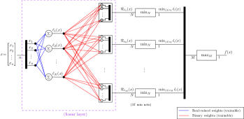
Figure 1. Illustration of TLL NN architecture for a function $\mathbb{R}^{n}\rightarrow\mathbb{R}$; reproduced from (Ferlez and Shoukry, 2020a). More details in Section 2.3.

Through extensive experiments, Fast BATLLNN exemplifies that sacrificing generality in both of these senses can lead to dramatically faster verification times. Compared to state-of-the-art general NN verifiers, Fast BATLLNN is 400-1900x faster verifying the same TLL NNs and properties.

In this sense, Fast BATLLNN  is primarily inspired by the recent result (Ferlez and Shoukry, 2020b), which showed that verifying a Two-Level Lattice (TLL) NN is an “easier” problem than verifying a general deep NN. Specifically, (Ferlez and Shoukry, 2020b) exhibits a polynomial time algorithm to verify a TLL with respect to an arbitrary half-space output property (i.e. polynomial-time in the number of neurons). Indeed, the semantic structure of the TLL architecture is precisely what makes polynomial-time verification possible: in a TLL NN, the neuronal parameters provide direct (polynomial-time) access to each of the affine functions that appear in its response, viewed as a Continuous Piecewise Affine (CPWA) function (Ferlez and Shoukry, 2020b). Since the same cannot be said of the neuronal parameters in a general deep NN, this indicates that considering only TLL NNs can facilitate a much faster verifier.

Thus, the major contribution of Fast BATLLNN is to further leverage the semantics of the TLL architecture under the additional assumption of verifying box-type (or hyper-rectangle) output properties. In particular, a TLL NN implements (component-wise) $\min$ and $\max$ lattice operations to compute each of its real-valued output components (as illustrated in Figure 1; see also Section 2.3). This fact can be used to dramatically simplify the verification of box-like output properties, which are component-wise real-valued intervals – and hence mutually decoupled. Importantly, the algorithm proposed in (Ferlez and Shoukry, 2020b) cannot take advantage of these lattice operations in the same way, since it considers only general half-space properties, which naturally couple the various output components of the TLL NN. As a result, we can show that Fast BATLLNN has a big-O verification complexity whose crucial exponent is half the size of the analogous exponent in (Ferlez and Shoukry, 2020b). The performance consequences of this improvement are reflected in our experimental results.

Before we proceed further, it is appropriate to make a few remarks about the restrictions inherent to Fast BATLLNN. Between the two restrictions of significance – the restriction to TLL NNs and the restriction to box-like output properties – the former is apparently more onerous: box-like properties can be used to adaptively assess more complicated properties whenever box-like properties are themselves inadequate. However even the restriction to TLL NNs is less imposing than at first it may seem. On the one hand, it is known that TLL NNs are capable of representing any Continuous Piecewise-Affine (CPWA) function (Ferlez and Shoukry, 2020a; Tarela and Martínez, 1999); i.e., any function that continuously switches between a finite set of affine functions. Since deep NNs themselves realize CPWA functions, the TLL NN architecture is able to instantiate any function that a generic deep NN can. We do not consider the problem of converting a deep NN to the TLL architecture (nor the possible loss in parametric efficiency that may result), but the extremely fast verification times achievable with Fast BATLLNN suggest that the trade off is very likely worth the cost. On the other hand, there is a spate of results which suggest that the TLL architecture a useful architecture within which to do closed-loop controller design in the first place (Ferlez and Shoukry, 2020a; Cruz et al., 2021; Ferlez et al., 2020) – potentially obviating the need for such a conversion at all.

Related work: To the best of our knowledge, the work (Ferlez and Shoukry, 2020b) is the only current example of an attempt to verify a specific NN architecture rather than a generic deep NN.

The literature on more general NN verifiers is far richer. These NN verifiers can generally be grouped into three categories: (i) SMT-based methods, which encode the problem into a Satisfiability Modulo Theory problem (Ehlers, 2017; Katz et al., 2017, 2019); (ii) MILP-based solvers, which directly encode the verification problem as a Mixed Integer Linear Program (Anderson et al., 2020; Bastani et al., 2016; Bunel et al., 2020; Cheng et al., 2017; Fischetti and Jo, 2018; Lomuscio and Maganti, 2017; Tjeng et al., 2017); (iii) Reachability based methods, which perform layer-by-layer reachability analysis to compute the reachable set (Bak et al., 2020; Fazlyab et al., 2019; Gehr et al., 2018; Ivanov et al., 2019; Tran et al., 2020a; Wang et al., 2018b; Xiang et al., 2017, 2018); and (iv) convex relaxations methods (Dvijotham et al., 2018; Wang et al., 2018a; Wong and Kolter, 2017; Khedr et al., 2020). Methods in categories (i) - (iii) tend to suffer from poor scalability, especially relative to convex relaxation methods. In this paper, we perform comparisons with state-of-the-art examples from category (iv) (Khedr et al., 2020; Wang et al., 2021) and category (iii) (Bak et al., 2020), as perform well overall in the standard verifier competition (vnn, [n. d.]).

2. Preliminaries

2.1. Notation

We will denote the real numbers by $\mathbb{R}$. For an $(n\times m)$ matrix (or vector), $A$, we will use the notation $\llbracket A\rrbracket_{[i,j]}$ to denote the element in the $i^{\text{th}}$ row and $j^{\text{th}}$ column of $A$. Analogously, the notation $\llbracket A\rrbracket_{[i,:]}$ will denote the $i^{\text{th}}$ row of $A$, and $\llbracket A\rrbracket_{[:,j]}$ will denote the $j^{\text{th}}$ column of $A$; when $A$ is a vector instead of a matrix, both notations will return a scalar corresponding to the corresponding element in the vector. We will use bold parenthesis $\;\negthinspace\text{{\stixfrak\char 54\relax}}\cdot\text{{\stixfrak\char 55\relax}}$ to delineate the arguments to a function that returns a function. We use two special forms of this notation: for an $(m\times n)$ matrix, $W$, and an $(m\times 1)$ vector, $b$:

(1) $$\mathscr{L}\negthinspace\text{{\stixfrak\char 54\relax}}W,b\text{{\stixfrak\char 55\relax}} :x\mapsto Wx+b$$

(2) $$\mathscr{L}_{i}\negthinspace\text{{\stixfrak\char 54\relax}}W,b\text{{\stixfrak\char 55\relax}} :x\mapsto\llbracket W\rrbracket_{[i,:]}x+\llbracket b\rrbracket_{[i,1]}.$$

We also use the functions $\mathtt{First}$ and $\mathtt{Last}$ to return the first and last elements of an ordered list (or by overloading, a vector in $\mathbb{R}^{n}$). The function $\mathtt{Concat}$ concatenates two ordered lists, or by overloading, concatenates two vectors in $\mathbb{R}^{n}$ and $\mathbb{R}^{m}$ along their (common) nontrivial dimension to get a third vector in $\mathbb{R}^{n+m}$. Finally, an over-bar indicates (topological) closure of a set: i.e. $\mkern 3.0mu\overline{\mkern-2.5muA\mkern-2.0mu}\mkern 2.0mu$ is the closure of $A$.

2.2. Neural Networks

We will exclusively consider Rectified Linear Unit Neural Networks (ReLU NNs). A $K$-layer ReLU NN is specified by $K$ layer functions, $\{L_{\theta^{|i}}:i=1,\dots,K\}$, of which we allow two kinds: linear and nonlinear. A nonlinear layer is a function:

(3) $$L_{\theta^{|i}}:\mathbb{R}^{\mathfrak{i}}\rightarrow\mathbb{R}^{\mathfrak{o}},\qquad L_{\theta^{|i}}:z\mapsto\max\{Wz+b,0\}$$

where the $\max$ function is taken element-wise, $W^{|i}$ and $b^{|i}$ are matrices of appropriate dimensions, and $\theta^{|i}\triangleq(W^{|i},b^{|i})$. A linear layer is the same as a nonlinear layer, except it omits the nonlinearity $\max\{\cdot,0\}$ in its layer function; a linear layer will be indicated with a superscript lin e.g. $L^{\text{lin}}_{\theta^{|i}}$ Thus, a $K$-layer ReLU NN function is specified by functionally composing $K$ such layer functions whose input and output dimensions satisfy $\mathfrak{i}_{i}=\mathfrak{o}_{i-1}:i=2,\dots,K$. We always consider the final layer to be a linear layer, so we may define:

(4) $${\mathscr{N}\negthickspace\negthickspace\negthinspace\mathscr{N}}\negthinspace=L_{\theta^{|K}}^{\text{lin}}\circ L_{\theta^{|K-1}}^{\vphantom{\text{lin}}}\circ\dots\circ L_{\theta^{|1}}^{\vphantom{\text{lin}}}$$

To make the dependence on parameters explicit, we will index a ReLU function ${\mathscr{N}\negthickspace\negthickspace\negthinspace\mathscr{N}}\negthinspace$ by a list of matrices $\Theta\triangleq$ $(\theta^{|1},$ $\dots,$ $\theta^{|K});$ in this respect, we will often use ${\mathscr{N}\negthickspace\negthickspace\negthinspace\mathscr{N}}\negthinspace={\mathscr{N}\negthickspace\negthickspace\negthinspace\mathscr{N}}\negthinspace\negthinspace\text{{\stixfrak\char 54\relax}}\Theta\text{{\stixfrak\char 55\relax}}$.

2.3. Two-Level-Lattice (TLL) Neural Networks

In this paper, we are exclusively concerned Two-Level Lattice (TLL) ReLU NNs as noted above. In this subsection, we formally define NNs with the TLL architecture using the succinct method exhibited in (Ferlez and Shoukry, 2020b); the material in this subsection is derived from (Ferlez and Shoukry, 2020a, b).

The most efficient way to characterize a TLL NN is by way of three generic NN composition operators. Hence, we have the following three definitions, which serve as auxiliary results in order to eventually define a TLL NN in Definition 4.

Definition 0 (Sequential (Functional) Composition).

Let ${\mathscr{N}\negthickspace\negthickspace\negthinspace\mathscr{N}}\negthinspace\negthinspace\text{{\stixfrak\char 54\relax}}\Theta_{\scriptscriptstyle 1}\text{{\stixfrak\char 55\relax}}:\mathbb{R}^{\mathfrak{i}}\rightarrow\mathbb{R}^{\mathfrak{c}}$ and ${\mathscr{N}\negthickspace\negthickspace\negthinspace\mathscr{N}}\negthinspace\negthinspace\text{{\stixfrak\char 54\relax}}\Theta_{\scriptscriptstyle 2}\text{{\stixfrak\char 55\relax}}:\mathbb{R}^{\mathfrak{c}}\rightarrow\mathbb{R}^{\mathfrak{o}}$ be two NNs. Then the sequential (or functional) composition of ${\mathscr{N}\negthickspace\negthickspace\negthinspace\mathscr{N}}\negthinspace\negthinspace\text{{\stixfrak\char 54\relax}}\Theta_{\scriptscriptstyle 1}\text{{\stixfrak\char 55\relax}}$ and ${\mathscr{N}\negthickspace\negthickspace\negthinspace\mathscr{N}}\negthinspace\negthinspace\text{{\stixfrak\char 54\relax}}\Theta_{\scriptscriptstyle 2}\text{{\stixfrak\char 55\relax}}$, i.e. ${\mathscr{N}\negthickspace\negthickspace\negthinspace\mathscr{N}}\negthinspace\negthinspace\text{{\stixfrak\char 54\relax}}\Theta_{\scriptscriptstyle 1}\text{{\stixfrak\char 55\relax}}\circ{\mathscr{N}\negthickspace\negthickspace\negthinspace\mathscr{N}}\negthinspace\negthinspace\text{{\stixfrak\char 54\relax}}\Theta_{\scriptscriptstyle 2}\text{{\stixfrak\char 55\relax}}$, is a well defined NN, and can be represented by the parameter list $\Theta_{1}\circ\Theta_{2}\triangleq\mathtt{Concat}(\Theta_{1},\Theta_{2})$.

Definition 0.

Let ${\mathscr{N}\negthickspace\negthickspace\negthinspace\mathscr{N}}\negthinspace\negthinspace\text{{\stixfrak\char 54\relax}}\Theta_{\scriptscriptstyle 1}\text{{\stixfrak\char 55\relax}}$ and ${\mathscr{N}\negthickspace\negthickspace\negthinspace\mathscr{N}}\negthinspace\negthinspace\text{{\stixfrak\char 54\relax}}\Theta_{\scriptscriptstyle 2}\text{{\stixfrak\char 55\relax}}$ be two $K$-layer NNs with parameter lists:

(5) $$\Theta_{i}=((W^{\scriptscriptstyle|1}_{i},b^{\scriptscriptstyle|1}_{i}),\dots,(W^{\scriptscriptstyle|K}_{i},b^{\scriptscriptstyle|K}_{i})),\quad i=1,2.$$

Then the parallel composition of ${\mathscr{N}\negthickspace\negthickspace\negthinspace\mathscr{N}}\negthinspace\negthinspace\text{{\stixfrak\char 54\relax}}\Theta_{\scriptscriptstyle 1}\text{{\stixfrak\char 55\relax}}$ and ${\mathscr{N}\negthickspace\negthickspace\negthinspace\mathscr{N}}\negthinspace\negthinspace\text{{\stixfrak\char 54\relax}}\Theta_{\scriptscriptstyle 2}\text{{\stixfrak\char 55\relax}}$ is a NN given by the parameter list

(6) $$\Theta_{1}\parallel\Theta_{2}\triangleq\big{(}\negthinspace\left(\negthinspace\left[\begin{smallmatrix}W^{\scriptscriptstyle|1}_{1}\\ W^{\scriptscriptstyle|1}_{2}\end{smallmatrix}\right],\left[\begin{smallmatrix}b^{\scriptscriptstyle|1}_{1}\\ b^{\scriptscriptstyle|1}_{2}\end{smallmatrix}\right]\negthinspace\right),{\scriptstyle\dots},\left(\negthinspace\left[\begin{smallmatrix}W^{\scriptscriptstyle|K}_{1}\\ W^{\scriptscriptstyle|K}_{2}\end{smallmatrix}\right],\left[\begin{smallmatrix}b^{\scriptscriptstyle|K}_{1}\\ b^{\scriptscriptstyle|K}_{2}\end{smallmatrix}\right]\negthinspace\right)\negthinspace\big{)}.$$

That is $\Theta_{1}\negthickspace\parallel\negthickspace\Theta_{2}$ accepts an input of the same size as (both) $\Theta_{1}$ and $\Theta_{2}$, but has as many outputs as $\Theta_{1}$ and $\Theta_{2}$ combined.

Definition 0 ($n$-element $\min$/$\max$ NNs).

An $n$-element $\min$ network is denoted by the parameter list $\Theta_{\min_{n}}$. ${\mathscr{N}\negthickspace\negthickspace\negthinspace\mathscr{N}}\negthinspace\negthinspace\text{{\stixfrak\char 54\relax}}\Theta_{\min_{n}}\text{{\stixfrak\char 55\relax}}:\mathbb{R}^{n}\rightarrow\mathbb{R}$ such that ${\mathscr{N}\negthickspace\negthickspace\negthinspace\mathscr{N}}\negthinspace\negthinspace\text{{\stixfrak\char 54\relax}}\Theta_{\min_{n}}\text{{\stixfrak\char 55\relax}}(x)$ is the minimum from among the components of $x$ (i.e. minimum according to the usual order relation $<$ on $\mathbb{R}$). An $n$-element $\max$ network is denoted by $\Theta_{\max_{n}}$, and functions analogously. These networks are described in (Ferlez and Shoukry, 2020a).

With Definition 1 through Definition 3 in hand, it is now possible for us to define TLL NNs in just the same way as (Ferlez and Shoukry, 2020b). We likewise proceed to first define a scalar (or real-valued) TLL NN; the structure of such a scalar TLL NN is illustrated in Figure 1. Then we extend this notion to a multi-output (or vector-valued) TLL NN.

Definition 0 (Scalar TLL NN (Ferlez and Shoukry, 2020b)).

A NN that maps $\mathbb{R}^{n}\rightarrow\mathbb{R}$ is said to be TLL NN of size $(N,M)$ if the size of its parameter list $\Xi_{\scriptscriptstyle N,M}$ can be characterized entirely by integers $N$ and $M$ as follows.

(7) $$\Xi_{N,M}\negthinspace\triangleq\negthinspace\Theta_{\max_{M}}\negthinspace\negthinspace\circ\negthinspace\big{(}(\negthinspace\Theta_{\min_{N}}\negthinspace\circ\Theta_{S_{1}}\negthinspace)\negthinspace\parallel\negthinspace{\scriptstyle\dots}\negthinspace\parallel\negthinspace(\negthinspace\Theta_{\min_{N}}\negthinspace\circ\Theta_{S_{M}}\negthinspace)\big{)}\negthinspace\circ\Theta_{\ell}$$

where

• $\Theta_{\ell}\triangleq((W_{\ell},b_{\ell}))$;

• each $\Theta_{S_{j}}$ has the form $\Theta_{S_{j}}=\big{(}S_{j},\mathbf{0}_{N,1}\big{)}$; and

• $S_{j}=\left[\begin{smallmatrix}{\llbracket I_{N}\rrbracket_{[\iota_{1},:]}}\negthickspace\negthickspace\negthickspace^{{}^{\scriptscriptstyle\text{T}}}&\;\dots\;&{\llbracket I_{N}\rrbracket_{[\iota_{N},:]}}\negthickspace\negthickspace\negthickspace^{{}^{\scriptscriptstyle\text{T}}}\end{smallmatrix}\right]^{\text{T}}$ for some length-$N$ sequence $\{\iota_{k}\}\subseteq\{1,\dots,N\}$ where $I_{N}$ is the $(N\times N)$ identity matrix.

The linear functions implemented by the mapping $\mathscr{L}_{i}\negthinspace\text{{\stixfrak\char 54\relax}}W_{\ell},b_{\ell}\text{{\stixfrak\char 55\relax}}$ for $i=1,\dots,N$ will be referred to as the local linear functions of $\Xi_{N,M}$; we assume for simplicity that these linear functions are unique. The matrices $\{S_{j}|j=1,\dots,M\}$ will be referred to as the selector matrices of $\Xi_{N,M}$. Each set $s_{j}\triangleq\{k\in\{1,\dots,N\}|\exists\iota\in\{1,\dots,N\}.\llbracket S_{j}\rrbracket_{\iota,k}=1\}$ is said to be the selector set of $S_{j}$.

Definition 0 (Multi-output TLL NN (Ferlez and Shoukry, 2020b)).

A NN that maps $\mathbb{R}^{n}\rightarrow\mathbb{R}^{m}$ is said to be a multi-output TLL NN of size $(N,M)$ if its parameter list $\Xi_{\scriptscriptstyle N,M}^{(m)}$ can be written as

(8) $$\Xi_{\scriptscriptstyle N,M}^{(m)}=\Xi_{\scriptscriptstyle N,M}^{1}\parallel\dots\parallel\Xi_{\scriptscriptstyle N,M}^{m}$$

for $m$ equally-sized scalar TLL NNs, $\Xi_{\scriptscriptstyle N,M}^{1},\dots,\Xi_{\scriptscriptstyle N,M}^{m}$; these scalar TLLs will be referred to as the (output) components of $\Xi_{\scriptscriptstyle N,M}^{(m)}$.

2.4. Hyperplanes and Hyperplane Arrangements

Here we review notation for hyperplanes and hyperplane arrangements; these results will be important in the developemnt of Fast BATLLNN. (Stanley, [n. d.]) is the main reference for this section.

Definition 0 (Hyperplanes and Half-spaces).

Let $\ell:\mathbb{R}^{n}\rightarrow\mathbb{R}$ be an affine map. Then define:

(9) $$H^{q}_{\ell}\triangleq\begin{cases}\{x|\ell(x)<0\}&q=-1\\ \{x|\ell(x)>0\}&q=+1\\ \{x|\ell(x)=0\}&q=0.\end{cases}$$

We say that $H^{0}_{\ell}$ is the hyperplane defined by $\ell$ in dimension $n$, and $H^{-1}_{\ell}$ and $H^{+1}_{\ell}$ are the negative and positive half-spaces defined by $\ell$, respectively.

Definition 0 (Hyperplane Arrangement).

Let $\mathcal{L}$ be a set of affine functions where each $\ell\in\mathcal{L}:\mathbb{R}^{n}\rightarrow\mathbb{R}$. Then $\{H^{0}_{\ell}|\ell\in\mathcal{L}\}$ is an arrangement of hyperplanes in dimension $n$.

Definition 0 (Region of a Hyperplane Arrangement).

Let $\mathcal{H}$ be an arrangement of $N$ hyperplanes in dimension $n$ defined by a set of affine functions, $\mathcal{L}$. Then a non-empty open subset $R\subseteq\mathbb{R}^{n}$ is said to be a region of $\mathcal{H}$ if there is an indexing function $\mathfrak{s}:\mathcal{L}\rightarrow\{-1,0,+1\}$ such that $R=\bigcap_{\ell\in\mathcal{L}}H^{\mathfrak{s}(\ell)}_{\ell}$; $R$ is said to be $n$-dimensional or full-dimensional if it is non-empty and described by an indexing function $\mathfrak{s}(\ell)\in\{-1,+1\}$ for all $\ell\in\mathcal{L}$.

Theorem 9 ((Stanley, [n. d.])).

Let $\mathcal{H}$ be an arrangement of $N$ hyperplanes in dimension $n$. Then $|\mathcal{R}_{\mathcal{H}}|$ is at most $\sum_{k=0}^{n}{N\choose k}$.

Remark 1.

Note that for a fixed dimension, $n$, the bound $\sum_{k=0}^{n}\negthinspace{N\choose k}$ grows like $O(N^{n}\negthinspace/n!)$, i.e. sub-exponentially in $N$.

3. Problem Formulation

The essence of Fast BATLLNN is its focus on verifying TLL NNs with respect to box-like output constraints. Formally, Fast BATLLNN considers only verification problems of the following form (stated using notation from Section 2).

Problem 1.

Let ${\mathscr{N}\negthickspace\negthickspace\negthinspace\mathscr{N}}\negthinspace\negthinspace\text{{\stixfrak\char 54\relax}}\Xi_{\scriptscriptstyle N,M}^{(m)}\text{{\stixfrak\char 55\relax}}:\mathbb{R}^{n}\rightarrow\mathbb{R}^{m}$ be a multi-output TLL NN. Also, let:

• $P_{X}\subset\mathbb{R}^{n}$ be a closed, convex polytope specified by the intersection of $\mathsf{N}_{X}$ half-spaces, i.e. $P_{X}\triangleq\cap_{i=1}^{\mathsf{N}_{X}}\{x:\ell_{X,i}(x)\leq 0\}$ where each $\ell_{X,i}:\mathbb{R}^{n}\rightarrow\mathbb{R}$ is affine; and

• $P_{Y}\subset\mathbb{R}^{m}$ be closed hyper-rectangle, i.e. $P_{Y}\triangleq\prod_{k=1}^{m}[a_{k},b_{k}]$ with $-\infty\leq a_{k}\leq b_{k}\leq\infty$ for each $k$.

Then the verification problem is to decide whether the following formula is true:

(10) $$\forall x\in P_{X}\subset\mathbb{R}^{n}.\big{(}{\mathscr{N}\negthickspace\negthickspace\negthinspace\mathscr{N}}\negthinspace\negthinspace\text{{\stixfrak\char 54\relax}}\Xi_{\scriptscriptstyle N,M}^{(m)}\text{{\stixfrak\char 55\relax}}\negthinspace(x)\in P_{Y}\subset\mathbb{R}^{m}\big{)}.$$

If (10) is true, the problem is SAT; otherwise, it is UNSAT.

Note that the properties (and their interpretations) in 1 are dual to the usual convention; it is more typical in the literature to associate “unsafe” outputs with a closed, convex polytope, and then the existence of such unsafe outputs is denoted by UNSAT (see (Tran et al., 2019) for example). However, we chose this formulation for 1 because it is the one adopted by (Ferlez and Shoukry, 2020b), and because it is more suited to NN reachability computations, one of the motivating applications of Fast BATLLNN. Indeed, to verify a property like (10), the typical dual formulation of 1 would require $2\cdot m$ verifier calls, assuming unbounded polytopes are verifiable (and then the verification would only be respect to the interior of $P_{Y}$). Of course this choice comes with a trade-off: Fast BATLLNN, which directly solves 1, requires adaptation to verify the dual property of 1; we return to this briefly at the end of this section, but it is ultimately left for future work.

In the case of Fast BATLLNN, there is another important reason to consider the stated formulation of 1: both the output property $P_{Y}$ and the NN $\Xi_{\scriptscriptstyle N,M}^{(m)}$ have an essentially component-wise nature (see also Definition 5). As a result, a component-wise treatment of 1 greatly facilitates the development and operation of Fast BATLLNN. To this end, we will find it convenient in the sequel to consider the following two verification problems; each is specified for a scalar TLL NNs and a single real-valued output property. Moreover, we cast them in terms of the negation of the analogous formula derived from 1; the reasons for this will become clear in Section 4.

Problem 1A (Scalar Upper Bound).

Let ${\mathscr{N}\negthickspace\negthickspace\negthinspace\mathscr{N}}\negthinspace\negthinspace\text{{\stixfrak\char 54\relax}}\Xi_{\scriptscriptstyle N,M}\text{{\stixfrak\char 55\relax}}:\mathbb{R}^{n}\rightarrow\mathbb{R}$ be a scalar TLL NN, and let $P_{X}\triangleq\cap_{i=1}^{\mathsf{N}_{X}}\{x:\ell_{X,i}(x)\leq 0\}$ be a closed convex polytope as in 1.

Then the scalar upper bound verification problem for $a\in\mathbb{R}$ is to decide whether the following formula is true:

(11) $$\exists x\in P_{X}\subset\mathbb{R}^{n}.\big{(}{\mathscr{N}\negthickspace\negthickspace\negthinspace\mathscr{N}}\negthinspace\negthinspace\text{{\stixfrak\char 54\relax}}\Xi_{\scriptscriptstyle N,M}\text{{\stixfrak\char 55\relax}}\negthinspace(x)>b\big{)}.$$

If (11) is true, the problem is UNSAT; otherwise, it is SAT.

Problem 1B (Scalar lower Bound).

Let ${\mathscr{N}\negthickspace\negthickspace\negthinspace\mathscr{N}}\negthinspace\negthinspace\text{{\stixfrak\char 54\relax}}\Xi_{\scriptscriptstyle N,M}\text{{\stixfrak\char 55\relax}}:\mathbb{R}^{n}\rightarrow\mathbb{R}$ and $P_{X}$ be as in 1A.

Then the scalar lower bound verification problem for $b\in\mathbb{R}$ is to decide whether the following formula is true:

(12) $$\exists x\in P_{X}\subset\mathbb{R}^{n}.\big{(}{\mathscr{N}\negthickspace\negthickspace\negthinspace\mathscr{N}}\negthinspace\negthinspace\text{{\stixfrak\char 54\relax}}\Xi_{\scriptscriptstyle N,M}\text{{\stixfrak\char 55\relax}}\negthinspace(x)<a\big{)}.$$

If (12) is true, the problem is UNSAT; otherwise, it is SAT.

Thus, note that the formulation of 1 is such that it can be verified by evaluating a boolean formula that contains only instances of 1A and 1B. That is, the following formula has the same truth value as (10):

(13) $$\bigwedge_{k=1}^{m}\Bigg{(}\neg\Big{(}\exists x\in P_{X}\subset\mathbb{R}^{n}.\big{(}{\mathscr{N}\negthickspace\negthickspace\negthinspace\mathscr{N}}\negthinspace\negthinspace\text{{\stixfrak\char 54\relax}}\Xi_{\scriptscriptstyle N,M}^{k}\text{{\stixfrak\char 55\relax}}\negthinspace(x)<a_{k}\big{)}\Big{)}\quad\wedge\\[-10.0pt] \neg\Big{(}\exists x\in P_{X}\subset\mathbb{R}^{n}.\big{(}{\mathscr{N}\negthickspace\negthickspace\negthinspace\mathscr{N}}\negthinspace\negthinspace\text{{\stixfrak\char 54\relax}}\Xi_{\scriptscriptstyle N,M}^{k}\text{{\stixfrak\char 55\relax}}\negthinspace(x)<b_{k}\big{)}\Big{)}\Bigg{)}.$$

We reiterate, however, that the same is not true of the dual property to 1. Consequently, Fast BATLLNN requires modification to verify such properties; this is a more or less straightforward procedure, but we defer this to future work, as noted above.

4. Fast BATLLNN: Theory

In this section, we develop the theoretical underpinnings of Fast BATLLNN. As noted in Section 3, the essential insight of our algorithm is captured by our solutions to problems 1A and 1B. Thus, this section is organized primarily around solving sub-problems of these forms; at the end of this section, we will show how to combine these results into a verification algorithm for 1, and then we will analyze the overall computational complexity of Fast BATLLNN.

4.1. Verifying 1A

1A, as stated above, regards the TLL NN to be verified merely as a map from inputs to outputs; this is the behavior that we wish to verify, after all. However, this point of view obscures the considerable semantic structure intrinsic to the neurons in a TLL NN. In particular, recall that ${\mathscr{N}\negthickspace\negthickspace\negthinspace\mathscr{N}}\negthinspace\negthinspace\text{{\stixfrak\char 54\relax}}\Xi_{\scriptscriptstyle N,M}\text{{\stixfrak\char 55\relax}}$ implements the following function, which was derived from the Two-Level Lattice representation of CPWAs – see Section 2.3 and (Ferlez and Shoukry, 2020a; Tarela and Martínez, 1999):

(14) $${\mathscr{N}\negthickspace\negthickspace\negthinspace\mathscr{N}}\negthinspace\negthinspace\text{{\stixfrak\char 54\relax}}\Xi_{\scriptscriptstyle N,M}\text{{\stixfrak\char 55\relax}}(x)=\max_{1\leq j\leq M}\min_{i\in s_{j}}\mathscr{L}_{i}\negthinspace\text{{\stixfrak\char 54\relax}}W_{\ell},b_{\ell}\text{{\stixfrak\char 55\relax}}(x).$$

In (14), the sets $s_{j}$ are the selector sets of ${\mathscr{N}\negthickspace\negthickspace\negthinspace\mathscr{N}}\negthinspace\negthinspace\text{{\stixfrak\char 54\relax}}\Xi_{\scriptscriptstyle N,M}\text{{\stixfrak\char 55\relax}}$ and the $\mathscr{L}_{i}\negthinspace\text{{\stixfrak\char 54\relax}}W_{\ell},b_{\ell}\text{{\stixfrak\char 55\relax}}$ are the local linear functions of ${\mathscr{N}\negthickspace\negthickspace\negthinspace\mathscr{N}}\negthinspace\negthinspace\text{{\stixfrak\char 54\relax}}\Xi_{\scriptscriptstyle N,M}\text{{\stixfrak\char 55\relax}}$; both terminologies are formally defined in Definition 4. Upon substituting (14) into (11), we obtain the following, far more helpful representation of the property expressed in 1A:

(15) $$\exists x\in P_{X}\subset\mathbb{R}^{n}.\big{(}\max_{1\leq j\leq M}\min_{i\in s_{j}}\mathscr{L}_{i}\negthinspace\text{{\stixfrak\char 54\relax}}W_{\ell},b_{\ell}\text{{\stixfrak\char 55\relax}}(x)>b\big{)}.$$

Literally, (15) compares the output property of interest, $b\in\mathbb{R}$, with a combination of real-valued $\max/\min$ operations applied to scalar affine functions. Crucially, that comparison is made using the usual order relation on $\mathbb{R}$, $\geq$, which is exactly the same order relation upon which the $\max$ and $\min$ operations are based.

Thus, it is possible to simplify (15) as follows. First note that the result of the $\max$ operation in (15) can exceed $b$ on $P_{X}$ if and only if:

(16) $$\exists x\in P_{X}.\exists j\in\{1,\dots,M\}.\Big{(}\min_{i\in s_{j}}\mathscr{L}(W_{\ell},b_{\ell})(x)>b\Big{)}.$$

In turn, the result of any one of the $\min$ operations in (15) can exceed $b$ on $P_{X}$, and hence make (16) true, if and only if

(17) $$\exists x\in P_{X}.\forall i\in s_{j}.\Big{(}\mathscr{L}_{i}\negthinspace\text{{\stixfrak\char 54\relax}}W_{\ell},b_{\ell}\text{{\stixfrak\char 55\relax}}(x)>b\Big{)}.$$

In particular, (17) is actually an intersection of half spaces, some open and some closed: the open half spaces come from local linear functions that violate the property; and the closed half-spaces come from the input property, $P_{X}$ (see 1). Moreover, there are at most $M$ such intersections of relevance to 1A: one for each of the $j=1,\dots,M$ such $\min$ operations present in (15). Finally, note that linear feasibility problems consisting entirely of non-strict inequality constraints are easy to solve: this suggests that we should first amend the $>b$ inequality with $\geq b$ before proceeding.

Formally, these ideas are captured in the following proposition.

Proposition 0.

Consider an instance of 1A. Then that instance is UNSAT if and only if the set:

(18) $$\bigcup_{j=1,\dots,M}\left(\bigcap_{i\in s_{j}}\{x\negthinspace:\mathscr{L}_{i}\negthinspace\text{{\stixfrak\char 54\relax}}W_{\ell},b_{\ell}\text{{\stixfrak\char 55\relax}}>b\}\cap\bigcap_{i=1}^{\mathsf{N}_{X}}\{x:\negthinspace\ell_{X,i}(x)\leq 0\}\negthinspace\right)\neq\emptyset.$$

Or equivalently, if for at least one of the $j=1,\dots,M$, the linear feasibility problem specified by the constraints

(19) $$F_{j}\triangleq\begin{cases}\mathscr{L}_{i_{1}}\negthinspace\text{{\stixfrak\char 54\relax}}W_{\ell},b_{\ell}\text{{\stixfrak\char 55\relax}}(x)\geq b\\ \vdots\\ \mathscr{L}_{i_{|s_{j}|}}\negthinspace\text{{\stixfrak\char 54\relax}}W_{\ell},b_{\ell}\text{{\stixfrak\char 55\relax}}(x)\geq b\end{cases}\bigwedge\;\;\begin{cases}\ell_{X,1}(x)\leq 0\\ \vdots\\ \ell_{X,\mathsf{N}_{X}}(x)\leq 0\end{cases}$$

is feasible, and one of the following conditions is true:

• it has non-empty interior; or

• there is a feasible point that lies only on some subset of the $\{\ell_{X,i}:i=1,\dots,\mathsf{N}_{X}\}$.

Proof.

The first claim follows immediately from the manipulations described in (16) and (17). The second claim merely exhausts the possibilities for how the constraints $\mathcal{L}_{i}\negthinspace\text{{\stixfrak\char 54\relax}}W_{\ell},b_{\ell}\text{{\stixfrak\char 55\relax}}(x)>b$ can participate in a feasible set for the linear program given by $F_{j}$. ∎

Remark 2.

The conclusion of Proposition 1 also has the following important interpretation: the $\exists x.(\dots>b)$ property can be seen to “distribute across” the $\max/\min$ operations in (15), and upon doing so, it converts the lattice operation $\max$ into set union and the lattice operation $\min$ into set intersection. Furthermore, since a TLL NN is constructed from two levels of lattice operations applied to affine functions, the innermost lattice operation of $\min$ is converted into a set intersection of half-spaces — i.e., a linear feasibility problem.

Of course Proposition 1 also suggests a natural and obvious algorithm to verify an instance of 1A. The pseudocode for this algorithm appears as the function verifyScalarUB in Algorithm 1, and its correctness follows directly from Proposition 1. In particular, verifyScalarUB simply evaluates the feasibility of each set of constraints $F_{j},j=1,\dots,M$ in turn, until either a feasible problem is found or the list is exhausted. Then for each such feasible $F_{j}$, verifyScalarUB attempts to find an interior point of the feasible set to reconcile it with the desired inequalities in (18); failing that, it searches for a vertex of the feasible set where no output property constraints are active. In practice, these operations can be combined by operating on the feasible point returned by the original feasibility program: an LP can be used to maximize the value of each constraint activate in order to explore adjacent vertices. Note further that verifyScalarUB may not need to execute all $M$ possible linear programs for properties that are UNSAT: it can terminate early on the first “satisfied” linear program found.

1

2

3

4

5

6

input :   $b\in\mathbb{R}$, a upper bound to verify

 $\Xi_{\scriptscriptstyle N,M}$, parameters of a TLL NN to verify

 $L_{X}=\{\ell_{X,1},\dots,\ell_{X,\mathsf{N}_{X}}\}$, affine functions

     specifying an input constraint polytope, $P_{X}$

output :   Boolean ($\mathtt{True=SAT};\mathtt{False=UNSAT}$)

7 function verifyScalarUB($b$, $\Xi_{\scriptscriptstyle N,M}$, $L_{X}$)

8      

9      for $j=1,\dots,M$ do

10            

11            constraints $\leftarrow$ $[\big{(}\mathscr{L}_{i}\negthinspace\text{{\stixfrak\char 54\relax}}W_{\ell},b_{\ell}\text{{\stixfrak\char 55\relax}}(x)\geq b\big{)}$ for $i\in s_{j}]$

12            constraints.append($[\ell_{X,1}(x)\leq~{}0,\dots,\ell_{X,N_{X}}(x)\leq~{}0]$)

13            (sol, status) $\leftarrow$ SolveLinFeas(constraints)

14            if status $==$ Feasible then

15                   if all($[\mathscr{L}_{i}\negthinspace\text{{\stixfrak\char 54\relax}}W_{\ell},b_{\ell}\text{{\stixfrak\char 55\relax}}($ sol $)>b$ for $i=1\dots N]$)

16                   or FindInt(constraints) == True then

17                         return False

18                   end if

19                  

20             end if

21            

22       end for

23      return True

24 end

Algorithm 1 verifyScalarUB; i.e., solve 1A

4.2. Verifying 1B

Naturally, we start our consideration of 1B in very much the same way as 1A. However, given that 1B and 1A are in some sense dual, the result is not nearly as convenient. In particular, substituting (14) into (12), and attempting carry out the same sequence of manipulations that led to Proposition 1 results in the following formula:

(20) $$\bigcap_{j=1,\dots,M}\left(\bigcup_{i\in s_{j}}\{x:\mathscr{L}_{i}\negthinspace\text{{\stixfrak\char 54\relax}}W_{\ell},b_{\ell}\text{{\stixfrak\char 55\relax}}(x)<a\}\cap\bigcap_{i=1}^{\mathsf{N}_{X}}\{x:\negthinspace\ell_{X,i}(x)\leq 0\}\right)\neq\emptyset,$$

which has the same truth value as formula (12). Unfortunately, (20) is not nearly as useful as the result in Proposition 1: under the “dual” output constraint $<a$, set intersection and set union are switched relative to Proposition 1. As a consequence, (20) is not itself a direct formulation in terms of intersections of half-spaces — i.e., linear feasibility problems.

Nevertheless, rearranging (20) into the union-of-half-space-int-
ersections form of Proposition 1 is possible and profitable. Using basic set operations, it is possible to rewrite (20) in a union-of-intersections form as follows (the set intersection $P_{X}=\cap_{i=1}^{\mathsf{N}_{X}}\{x:\ell_{X,i}(x)\leq 0\}$ is moved outside the outer union for convenience):

(21) $$P_{X}\cap\bigcup_{\begin{smallmatrix}(i_{1},\dots,i_{M})\\ \in s_{1}\times\dots\times s_{M}\end{smallmatrix}}\bigcap_{k=1,\dots,M}\{x:\mathscr{L}_{i_{k}}\negthinspace\text{{\stixfrak\char 54\relax}}W_{\ell},b_{\ell}\text{{\stixfrak\char 55\relax}}(x)<a\}\neq\emptyset.$$

By construction, (21) again has the same truth value as (12), but it is now in the desired form. In particular, it is verifiable by evaluating a finite number of half-space intersections much like Proposition 1.

Unfortunately, as a result of this rearrangement, the total number of mutual half-space intersections – or intersection “terms” – has grown from $M$ to $\prod_{j=1}^{M}|s_{j}|$, where $|s_{j}|$ is the cardinality of the selector set, $s_{j}$. In particular, this number can easily exceed $M$: for example, if each of the $s_{j}$ has exactly two elements, then there are $2^{M}$ total mutual intersection terms. Thus, verifying (21) in its current form would appear to require (in the worst case) exponentially more linear feasibility programs than the verifier we proposed for 1A. This situation is not only non-ideal in terms of run-time: it would also seem to contradict (Ferlez and Shoukry, 2020b), which describes an algorithm with polynomial-time complexity in $N$ and $M$ — and that algorithm is after all applicable to more general output properties.

Fortunately, however, there is one aspect not emphasized in this analysis so far: these intersection terms consist of half-spaces, and moreover, each of the half-spaces therein is specified by a hyperplane chosen from among a single, common group of $N$ hyperplanes. This will ultimately allow us to identify each non-empty intersection term in (21) with a full, $n$-dimensional region from this hyperplane arrangement, and by Theorem 9 in Section 2.4, there are at most $O(N^{n}/n!)$ such regions. Effectively, then, the geometry of this hyperplane arrangement (with $N$ hyperplanes in dimension $n$) prevents exponential growth in the number intersection terms relevant to the truth of (21): indeed, the polynomial growth, $O(N^{n}/n!)$, means that many of those intersection terms cannot correspond to valid regions in the arrangement.

In particular, consider the following set of affine functions, which in turn defines an arrangement of hyperplanes in $\mathbb{R}^{n}$:

(22) $$l_{i}^{a}\triangleq\mathscr{L}_{i}\negthinspace\text{{\stixfrak\char 54\relax}}W_{\ell},b_{\ell}\text{{\stixfrak\char 55\relax}}-a.$$

Let $\mathfrak{h}_{a}\triangleq\cup_{i=1}^{N}\{H^{0}_{l_{i}^{b}}\}$ denote the corresponding arrangement. Now, consider any index $(i_{1},\dots,i_{M})\in s_{1}\times\dots\times s_{M}$ specifying an intersection term in (21), and suppose without loss of generality that $i_{1},\dots,i_{K}$ are the only unique indices therein (an assumption we carry forward). Then using the notation $H^{-1}$ introduced in Definition 6, it is straightforward to write:

(23) $$\bigcap_{k=1,\dots,M}\{x:\mathscr{L}_{i_{k}}\negthinspace\text{{\stixfrak\char 54\relax}}W_{\ell},b_{\ell}\text{{\stixfrak\char 55\relax}}(x)<a\}=\bigcap_{i=1}^{K}H^{-1}_{l_{i}^{a}},$$

and where $l_{i}^{a}$ is as defined in (22). As a consequence, we conclude:

(24) $$\bigcap_{k=1,\dots,M}\{x:\mathscr{L}_{i_{k}}\negthinspace\text{{\stixfrak\char 54\relax}}W_{\ell},b_{\ell}\text{{\stixfrak\char 55\relax}}(x)<a\}\neq\emptyset\\ \Leftrightarrow\exists(\mathfrak{s}^{\prime}:\{l_{i}^{a}:i=1,\dots,K\}\rightarrow\{-1\}).\Big{(}\bigcap_{i=1}^{K}H^{\mathfrak{s}^{\prime}(l_{i}^{a})}_{l_{i}^{a}}\neq\emptyset\Big{)}.$$

Although it seems unnecessary to introduce the function $\mathfrak{s}^{\prime}$, this notation directly connects (23) to full-dimensional regions of the arrangement $\mathfrak{h}_{a}$. Indeed, it states that the intersection term of interest is non-empty if and only if there is a full-dimensional region in the hyperplane arrangement whose index function $\mathfrak{s}:\{l_{i}^{a}:i=1,\dots N\}\rightarrow\{-1,+1\}$ agrees with one of the partial indexing functions $\mathfrak{s}^{\prime}$ described in (24). More simply, said intersection term is non-empty if and only if it contains a full-dimensional region from the arrangement $\mathfrak{h}_{a}$; such a region can be said to “witness” the non-emptiness of the intersection term. This idea is illustrated in Figure 2.

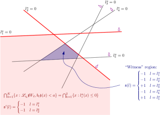
Figure 2. Illustration of identifying a non-empty intersection term from (21) with a full-dimensional region from the hyperplane arrangement $\mathfrak{h}_{a}$; positive half-spaces are indicated with blue arrows. Intersection term and defining half-spaces shown in red; “witness” region from $\mathfrak{h}_{a}$ shown in blue. Input constraints, $P_{X}$, omitted for clarity.

Formally, we have the following proposition.

Proposition 0.

Consider an instance of 1B. Then that instance is UNSAT if and only if the set:

(25) $$P_{X}\cap\bigcup_{\begin{smallmatrix}(i_{1},\dots,i_{M})\\ \in s_{1}\times\dots\times s_{M}\end{smallmatrix}}\bigcap_{k=1,\dots,M}\{x:\mathscr{L}_{i_{k}}\negthinspace\text{{\stixfrak\char 54\relax}}W_{\ell},b_{\ell}\text{{\stixfrak\char 55\relax}}(x)<a\}\neq\emptyset.$$

And this is the case if and only if there exists an index $(i_{1},\dots,i_{M})\in s_{1}\times\dots\times s_{M}$ with distinct elements denoted by $j_{1},\dots,j_{K}\in\{1,\dots,M\}$ such that the following holds:

• there exists a region $R$ in $\mathfrak{h}_{a}$, specified by $\mathfrak{s}_{R}:\{l_{i}^{a}:i=1,\dots,N\}\rightarrow\{-1,0,+1\}$, such that:

  (26) $$\mathfrak{s}_{R}(l^{a}_{j_{k}})=-1\text{ for all }k=1,\dots,K$$

  and

  (27) $$R\cap P_{X}\neq\emptyset.$$

If such a region $R$ exists, then it is said to witness the non-emptiness of the corresponding intersection term with the index $(i_{1},\dots,i_{M})$.

Proof.

The proof follows from the above manipulations. ∎

Proposition 2 establishes a crucial identification between full-dimensional regions in a hyperplane arrangement and the non-empty intersection terms in (21), a verification formula equivalent to the satisfiability of 1B. However, it is still framed in terms of individual indices of the form $(i_{1},\dots,i_{M})$, which are too numerous to enumerate for reasons noted above. Thus, converting Proposition 2 into a practical and fast algorithm to solve 1B entails one final step: efficiently evaluating a full-dimensional region in $\mathfrak{h}_{a}$ to determine if it matches any index of the form form $(i_{1},\dots,i_{M})\in s_{1}\times\dots\times s_{M}$. This will finally lead to Fast BATLLNN’s algorithm to verify an instance 1B by enumerating the regions of $\mathfrak{h}_{a}$ instead of enumerating all of the indices in $s_{1}\times\dots\times s_{M}$.

Predictably, Fast BATLLNN essentially takes a greedy approach to this problem. In particular, consider a full-dimensional region, $R\subset\mathbb{R}^{n}$, of the hyperplane arrangement $\mathfrak{h}_{a}$, and suppose that $R$ is specified by the index function (see Definition 8):

(28) $$\mathfrak{s}_{R}:\{l_{i}^{a}|i=1,\dots N\}\rightarrow\{-1,+1\}.$$

According to Proposition 2, $\mathfrak{s}_{R}$ will be a witness to a violation of 1B if each of its negative hyperplanes (those assigned $-1$ by $\mathfrak{s}_{R}$) can be matched to any element of one of the selector sets, $s_{j}$ $j=1,\dots,M$. Thus, to establish whether $\mathfrak{s}_{R}$ corresponds to a non-empty intersection term, we can iterate over its negative hyperplanes, checking each one for membership in any one of the $s_{j}$. This iteration proceeds as long as each negative hyperplane is found to be an element of some $s_{j}$. If all negative hyperplanes of $R$ can be matched in this way, then the region $R$ is a witness to a violation of 1B as per Proposition 2. If, however, a negative hyperplane of $R$ is found to belong to no $s_{j}$, then the iteration terminates, since the region $R$ cannot be a witness to a violation of 1B. This algorithm amounts to a greedy matching of the negative hyperplanes of $R$, and it works by effectively examining the smallest intersection term to which the region $R$ can be a witness. The pseudocode for this algorithm, with an outer loop to iterate over regions of $\mathfrak{h}_{a}$, appears as verifyScalarLB in Algorithm 2.

1

2

3

4

5

6

7

input :   $a\in\mathbb{R}$, a lower bound to verify

 $\Xi_{\scriptscriptstyle N,M}$, parameters of a TLL NN to verify

 $L_{X}=\{\ell_{X,1},\dots,\ell_{X,\mathsf{N}_{X}}\}$, affine functions

     specifying an input constraint polytope, $P_{X}$

output :   Boolean ($\mathtt{True=SAT};\mathtt{False=UNSAT}$)

8 function verifyScalarLB($a$, $\Xi_{\scriptscriptstyle N,M}$, $L_{X}$)

9      

10      h_a $\leftarrow$ $[\mathcal{L}_{i}\negthinspace\text{{\stixfrak\char 54\relax}}W_{\ell},b_{\ell}\text{{\stixfrak\char 55\relax}}(x)-a\;\;$ for $~{}i=1\dots N~{}]$

11      for reg in Regions(h_a) do

12            

13            if reg $\cap P_{X}==\emptyset$ then

14                   continue reg

15             end if

16            

17            negHypers $\leftarrow$ NegativeHyperplanes(reg)

18            for i in negHypers do

19                  

20                  for j $=1\dots M$ do

21                        

22                        if l(i,a) $\not\in s_{\text{{{j}}}}$ then

23                              

24                              /* This region cannot be a witness to violation; go to next region */

25                              

26                              continue reg

27                         end if

28                        

29                   end for

30                  

31                  /* This region witnesses a violation; return */

32                  

33                  return False

34             end for

35            

36       end for

37      return True

38 end

Algorithm 2 verifyScalarLB; i.e., solve 1B

4.3. On the Complexity of Fast BATLLNN

Given the remarks prefacing equation (13), it suffices to consider the complexity of Proposition 1 and 1B individually. To simplify the notation in this section, we denote the complexity of running a linear program with $N$ constraints in $n$ variables by $\mathtt{LP}(N,n)$. Note also: we consider complexities for a fixed $n$.

4.3.1. Complexity of 1A

Analyzing the complexity of verifyScalarUB in Algorithm 1 is straightforward. There are $M$ total $\min$ (or intersection) terms, and each of these requires: one LP to check for $\geq b$ feasibility (line 5 of Algorithm 1); followed by at most $N$ LPs to find an interior point (line 8 of Algorithm 1). Thus, the complexity of verifyScalarUB is bounded by the following:

(29) $$O(M\cdot N\cdot\mathtt{LP}(N+\mathsf{N}_{X},n).)$$

4.3.2. Complexity of 1B

Analyzing the runtime complexity of verifyScalarLB in Algorithm 2 is also more or less straightforward, given an algorithm that enumerates the regions of a hyperplane arrangement. Fast BATLLNN uses an algorithm very similar to the reverse search algorithm described in (Avis and Fukuda, 1996) and improved slightly in (Ferrez et al., 2001). For a hyperplane arrangement consisting of $N$ hyperplanes in dimension $n$, that reverse search algorithm has a per-region complexity bounded by:

(30) $$O(N\cdot\mathtt{LP}(N,n)).$$

By Theorem 9 in Section 2, there are at most $O(N^{n}/n!)$ such regions.

Indeed, the per-region complexity of the loops in verifyScalarLB is easily seen to be bounded by $M\cdot N^{2}$ operations per region. Thus, it remains to evaluate the complexity of checking the intersection $\mathtt{reg}\cap P_{X}==\emptyset$ (see line 4 of Algorithm 2); however, this only appears as a separate operation for pedagogical simplicity. Fast BATLLNN actually follows the technique in (Ferlez and Shoukry, 2020b) to achieve the same assertion: the hyperplanes describing $P_{X}$ are added to the arrangement $\mathfrak{h}_{a}$, and any region for which one of those hyperplanes satisfies $\mathfrak{s}(\ell_{X,i})=+1$ is ignored. This can be done with the additional per-region complexity associated with the size of the larger arrangement, but without increasing the number of regions evaluated beyond $O(N^{n}/n!)$. Thus, we claim the complexity of Algorithm 2 is bounded by:

(31) $$O\big{(}\;M\cdot N^{2}\cdot(N+\mathsf{N}_{X})\cdot\mathtt{LP}(N+\mathsf{N}_{X},n))\cdot(N^{n}/n!)\;\big{)}\\ =O(M\cdot N^{n+3}\cdot\mathtt{LP}(N+\mathsf{N}_{X},n)/n!).$$

4.3.3. Complexity of Fast BATLLNN Compared to (Ferlez and Shoukry, 2020b)

We begin by adapting the TLL verification complexity reported in (Ferlez and Shoukry, 2020b, Theorem 3) to the scalar TLLs and single output properties of 1A and 1B. In the notation of this paper, it is as follows:

(32) $$O(n\cdot M\cdot N^{2n+3}\cdot\mathtt{LP}(N^{2}+\mathsf{N}_{X},n)/n!).$$

It is immediately clear that Fast BATLLNN has a significant complexity advantage for either type of property. Even the more expensive verifyScalarLB has a runtime complexity of $\approx O(N^{n})$ compared to $\approx O(N^{2n})$ for (Ferlez and Shoukry, 2020b, Theorem 3), and that doesn’t even count the larger LPs used in (Ferlez and Shoukry, 2020b, Theorem 3).

5. Implementation

5.1. General Implementation

The core algorithms of Fast BATLLNN, Algorithm 1 and Algorithm 2, are amenable to considerable parallelism. Thus, in order to make Fast BATLLNN as fast as possible, its implementation is focused on parallelism and concurrency as much as possible.

With this in mind, Fast BATLLNN is implemented using a high-performance concurrency abstraction library for Python called charm4py (Cha, [n. d.]). charm4py uses an actor model to facilitate concurrent programming, and it provides a number of helpful features to achieve good performance with relatively little programming effort. For example, it employs a cooperative scheduler to eliminate race-conditions, and it transparently offers the standard Python pass-by-reference semantics for function calls on the same Processing Element (PE). Moreover, it can be compiled to run on top of Message Passing Interface (MPI), which allows a single code base to scale from an individual multi-core computer to a multi-computer cluster. Fast BATLLNN was written with the intention of being deployed this way: it offers flexibility in how its core algorithms are assigned PEs, so as to take better take advantage of both compute and memory resources that are spread across multiple computers.

5.2. Implementation Details for Algorithm 2

Between the two core algorithms of Fast BATLLNN, Algorithm 2 is the more challenging to parallelize. Indeed, Algorithm 1 has a trivial parallel implementation, since it consists primarily of a for loop over a known index set. In Algorithm 2, it is the for loop over regions of a hyperplane that makes parallelization non-trivial. Hence, this section describes how Fast BATLLNN parallelizes the region enumeration of a hyperplane arrangement for Algorithm 2.

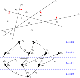
Figure 3. (Top) A hyperplane arrangement $\{H^{0}_{\ell_{1}},\dots,H^{0}_{\ell_{4}}\}$ with positive half spaces denoted by red arrows and regions $B,R_{1},\dots,R_{9}$. (Bottom) The corresponding adjacency poset.

To describe the architecture of Fast BATLLNN’s implementation of hyperplane region enumeration, we first briefly introduce the well-known reverse search algorithm for the same task (Ferrez et al., 2001), and the algorithm on which Fast BATLLNN’s implementation is loosely based. As its name suggests, it is a search algorithm: that is, it starts from a known region of the arrangement and searches for regions adjacent to it, and then regions adjacent to those, and so on. In particular, though, the reverse search algorithm is fundamentally a depth-first search, and it uses a minimum-index rule to ensure that regions are not visited multiple times (i.e., functioning much as Bland’s rule in simplex solvers) (Ferrez et al., 2001; Avis and Fukuda, 1996). This type of search algorithm has the great benefit that it is memory efficient, since it tracks the current state of the search using only the memory required to track adjacency indices; even the information required to back-track over the current branch is computed rather than being stored (Ferrez et al., 2001, pp. 10). However, the memory efficiency of (Ferrez et al., 2001) comes at the expense of parallelizability, precisely because the search state is stored using variables that are incremented with each descent down a branch.

The natural way to parallelize such a search is to allow multiple concurrent search workers, but have them enter their independent search results into a common, synchronized hash table. Assuming an amortized $O(1)$ hash complexity, this solution doesn’t affect the overall computational complexity; on the other hand, it comes with a steep memory penalty, since it could require storing all $O(N^{n})$ regions in the worst case. However, there is nevertheless a way to efficiently enable and coordinate multiple search processes, while avoiding this excessive memory requirement.

To this end, Fast BATLLNN leverages a special property of the region adjacency structure in a hyperplane arrangement. In particular, the regions of a hyperplane arrangement can be organized into a leveled adjacency poset (Edelman, 1984). That is, relative to any initial base region, all of the regions in the arrangement can be grouped according to the number of hyperplanes that were “crossed” in the process discovering them; the same idea is also implicit in (Ferrez et al., 2001; Avis and Fukuda, 1996). This leveled property of the adjacency poset is illustrated in Figure 3: the top pane shows a hyperplane arrangement with its regions labeled; the bottom pane depicts the region adjacency poset for this arrangement, with levels indicated relative to a base region, $B$. For example, a search starting from $B$ will find region $R_{1}$ by crossing only $\ell_{1}$ and region $R_{2}$ by crossing $\ell_{1}$ and $\ell_{3}$.

Thus, Fast BATLLNN still approaches the region enumeration problem as search, but instead it proceeds level-wise. All of the regions in the current level can be easily divided among the available processing elements, which then search in parallel for their immediately adjacent regions; the result of this search is a list of regions comprising the entire next level in the adjacency poset, which then becomes the current level and the process repeats. From an implementation standpoint, searching the region adjacency structure level-wise offers a useful way of reducing Fast BATLLNN’s memory footprint. In particular, once a level is fully explored, the regions it contains will never be seen again. Thus, Fast BATLLNN need only maintain a hash of regions from one level at a time: the hash tables from previous levels can be safely discarded. In this way, Fast BATLLNN achieves a parallel region search but without resorting to hashing the entire list of discovered regions.

Finally, we note that a search-type algorithm for region enumeration has a further advantage for solving a problem like 1B, though. In particular, a search algorithm reveals each new region with a relatively low computational cost — see (30); this is in contrast to some other enumeration algorithms, which must run to completion before even one region is available. Since Algorithm 2 is structured such that it can terminate on the first violating region found, this has a considerable advantage for UNSAT problems, as a violating region may be found very early in the search.

6. Experiments

We conducted a series of experiments to evaluate the performance and scalability of Fast BATLLNN as a TLL verifier, both in its own right and relative to general NN verifiers applied to TLL NNs. In particular, we conducted the following three experiments:

1. Scalability of Fast BATLLNN as a function of TLL input dimension, $n$; the number of local linear functions, $N$, and the number of selector sets, $M$, remained fixed.

2. Scalability of Fast BATLLNN as a function of the number of local linear functions, $N$, with $N=M$; the input dimension, $n$, remained fixed.

3. Comparison with general NN verifiers: nnenum (Bak et al., 2020), PeregriNN (Khedr et al., 2020) and Alpha-Beta-Crown (Wang et al., 2021).

All experiments were run within a VMWare Workstation Pro virtual machine (VM) running on a Linux host with 48 hyper-threaded cores and 256 GB of memory. All instances of the VM were given 64 GB of memory, and a core count that is specified within each experiment. A timeout of 300 seconds was used in all cases.

6.1. Experimental Setup: Networks and Properties

6.1.1. TLL NNs Verified

Given that 1 can be decomposed into instances of 1A and 1B, all of these experiments were conducted on scalar-output TLL NNs using real-valued properties of the form in either 1A or 1B.

In Experiments 1 and 2, TLL NNs of the desired $n$, $N$ and $M$ were generated randomly according to the following procedure, which was designed to ensure that they are unlikely to be degenerate on (roughly) the input set $[-1,1]^{n}$. The procedure is as follows:

1. Randomly generate elements of $W_{\ell}$ and $b_{\ell}$ according to normal distributions of mean zero and standard deviations of $1/10$ and $1$, respectively.

2. Randomly generate selector sets, $s_{j}$, by generating random integers between $0$ and $2^{N+1}-1$, and continue generating them by this mechanism until $M$ are obtained such that no two selector sets satisfy $s_{j}\subseteq s_{j^{\prime}}$ (a form of degeneracy).

3. For each corresponding selector matrix, $S_{j}$, solve $M$ instances of the following least squares problem:

   (33) $$\min_{x_{j}\in\mathbb{R}^{n}}\lVert S_{j}W_{\ell}x_{j}-S_{j}b_{\ell}\rVert_{2},$$

   to obtain the $M$ vectors, $x_{1},\dots,x_{M}$.

4. Then scale each row of $W_{\ell}$ (from (1) above) by the corresponding row of the vector:

   (34) $$\left[\begin{smallmatrix}\max_{j=1\dots M}|\llbracket x_{j}\rrbracket_{[1,1]}|&\dots&\max_{j=1\dots M}|\llbracket x_{j}\rrbracket_{[N,1]}|\end{smallmatrix}\right]^{\text{T}}.$$

   This has the (qualitative) effect of forcing the mutual intersections of randomly generated local linear functions to be concentrated around the origin.

In Experiment 3, we obtained and used the scalar TLL NNs that were tested in (Ferlez and Shoukry, 2020b). These networks all have $n=2$ and $N=M$; there are thirty examples for each of the sizes $N=M=8,16,24,32,40,48,56$ and $64$ (each size has a common neuron count, ranging from $256$ neurons for $N=8$ to $16384$ neurons for $N=64)$. We used these networks in particular so as to enable some basis of comparison with the experimental results in (Ferlez and Shoukry, 2020b). This is relevant, since that tool is not publicly available, and hence omitted from our comparison. Note: we considered these networks with different, albeit similar, properties to those used in (Ferlez and Shoukry, 2020b); see Section 6.1.3 below.

6.1.2. Input Constraints, $P_{X}$

In all experiments, we considered verification problems with $P_{X}=[-2,2]^{n}$. For the TLLs we generated, there is no great loss of generality in considering this fixed size for $P_{X}$, since we generated them to be “interesting” in this vicinity; see Section 6.1.1. However, using a hyper-rectangle $P_{X}$ was necessary for Experiment 3, since some of the general NN verifiers accept only hyper-rectangle input constraints. Thus, we made the universal choice $P_{X}=[-2,2]^{n}$ for consistency between experiments.

Note, however, that (Ferlez and Shoukry, 2020b) verified general polytopic input constraints on the networks we borrowed for Experiment 3. Nevertheless, we expect the results for Fast BATLLNN in Experiment 3 to be somewhat comparable to the results in (Ferlez and Shoukry, 2020b), since all of those polytopic constraints are contained in the box, $P_{X}=[-2,2]^{2}$.

6.1.3. Output Properties Verified

For a scalar TLL, only two parameters are required to specify an output property: a real-valued scalar and the direction of the inequality. In all cases, the direction of the inequality was determined by the outcome of Bernoulli random variable. And in all cases except one (noted in Experiment 2), the random real-valued property was generated by the following procedure. First, the TLL network was evaluated at 10,000 samples collected from the set $P_{X}$; any property between the min and max of these output samples is guaranteed to be UNSAT. Then, to get a mixture of SAT/UNSAT properties, we select a random property from this interval symmetrically extended to twice its original size.

6.2. Experiment 1: Input Dimension Scalability

In this experiment, we evaluated the scalability of Fast BATLLNN as a function of input dimension of the TLL to be verified. To that end, we generated a suite of TLL NNs with input sizes varying from $n=1$ to $n=30$, using the procedure described in Section 6.1.1. We generated 20 instances for each size, and for all TLLs, we kept $N=M=64$ constant. We then verified each of these TLLs with respect to its own, randomly generated property (as described in Section 6.1.3). For this experiment, Fast BATLLNN was run in a VM with 32 cores.

Figure 4 summarizes the results of this experiment with a box-and-whisker plot of verification times: each box-and-whisker summarizes the verification times for the twenty networks of the corresponding input dimension; no properties/networks resulted in a timeout. The data in the figure shows a clear trend of increasing median, as expected for progressively harder problems (recall the runtime complexities indicated in Section 4.3). By contrast, note that the minimum and maximum runtimes grow very slowly with dimension: given the complexity analysis of Section 4.3, we speculate that these results are likely due to the characteristics of the generated TLLs. That is, the generation procedure appears to “saturate” in the sense that it eventually produces networks which require, on average, a constant number of loop iterations to verify.

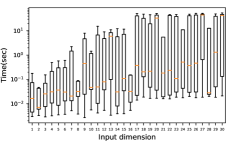
Figure 4. Experiment 1. Scaling the Input Dimension

6.3. Experiment 2: Network Size Scalability

In this experiment, we evaluated the scalability of Fast BATLLNN as a function of the number of local linear functions, $N$, in the TLL to be verified. To that end, we generated a suite of of TLL NNs local linear functions ranging in number from $N=16$ to $N=512$, again using the procedure described in Section 6.1.1. We generated 20 instances for each value of $N$, and for all networks we set $M=N$ and $n=15$. We then verified each of these networks with respect to its own, randomly generated property. The properties for network sizes $N=16$ through $N=256$ were generated as described in Section 6.1.3; however, a our TensorFlow implementation occupied too much memory to generate samples for TLLs of size $N=512$, so the properties for these networks were generated using the bounds for the $N=256$ TLLs. For this experiment, Fast BATLLNN was run in a VM with 32 cores.

Figure 5 summarized the results of this experiment with a box-and-whisker plot of verification times: each box-and-whisker summarize the verification times for the twenty test cases of the corresponding size, much as in Section 6.2. However, since some verification problems timed out in this experiment, those time outs were excluded from the box-and-whisker; they are instead indicated by a superimposed bar graph, which displays a count of the number of timeouts obtained from each group of equally-sized TLLs. The data in this figure shows the expected trend of increasingly difficult verification as $N$ increases; this is especially captured by the trend of experiencing more timeouts for larger networks. The outlier to this trend is the size $N=512$, but this is most likely due to different method of generating properties for these networks (see above). Finally, note that the minimum verification times exhibit a much slower growth trend, as in Experiment 1.

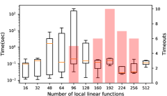
Figure 5. Experiment 2. Scaling the Number of Local Linear Functions

6.4. Experiment 3: General NN Verifiers

In this experiment, we compared the verification performance of Fast BATLLNN with state-of-the-art (SOTA) NN verifiers designed to work on general deep NNs. For this experiment, we compared against generic verifiers Alpha-Beta-Crown (Wang et al., 2021), nnenum (Bak et al., 2020) and PeregriNN (Khedr et al., 2020), as a representative sample of SOTA NN verifiers. Moreover, we conducted this experiment on the same 240 networks used in (Ferlez and Shoukry, 2020b), and described in Section 6.1.1; this further facilitates a limited comparison with that algorithm, subject to the caveats described in Section 6.1.1 and Section 6.1.3.

In order to make this test suite of TLLs available to the generic verifiers, each network was first implemented as a TensorFlow model using a custom implementation tool. The intent was to export these TensorFlow models to the ONNX format, which each of the generic verifiers can read. However, most of the generic verifiers do not support implementing multiple feed-forward paths by tensor reshaping operations, as in the most straightforward implementation of a TLL; see Figure 1 and Section 2.3. Thus, we had to first “flatten” our TensorFlow implementation into an equivalent network where each $\min$ network accepts the outputs of all of the selector matrices, only to null the irrelevant ones with additional kernel zeros in the first layer. This is highly sub-optimal, since it results in neurons receiving many more inputs than are really required. However, we could not devise another method to circumvent this limitation present in most of the tools.

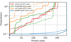
Figure 6. Experiment 3. General NN Verifiers

With all of the tools able to read the same NNs in our (borrowed) test suite, we randomly generated verification properties for each of the networks, as in the previous experiments. However, recall that the generic NN verifiers have a slightly different interpretation of properties compared with Fast BATLLNN. For scalar-output networks, this amounts to verifying the properties in 1A and 1B with the same interpretations, but with non-strict inequalities instead of strict inequalities. Since this will only generate divergent results when a property happens to be exactly equal to the maximum or minimum value on $P_{X}$, we elide this issue.

Thus, we ran each of the tools, Fast BATLLNN, Alpha-Beta-Crown, nnenum and PeregriNN on this test suite of TLLs and properties. PeregriNN was configured with SPLIT_RES = 0.1; nnenum was configured with TRY_QUICK_APPROX = True and all other parameters set to default values; and Alpha-Beta-Crown was configured with input space splitting, share_slopes = True, no_solve_slopes = True, lr_alpha = 0.01, and branching_method = sb. All the solvers used float64 computations. Furthermore, we ran two versions of this experiment, one where the VM had 4 cores and one where the VM had 24 cores.

Figure 6 summarizes the results of this experiment in the form of a cactus plot: a point on any one of the curves indicates the timeout that would be required to obtain the corresponding number of proved cases for that tool (from among of the test suite described above). As noted, each tool was run separately in two VMs, one with 4 cores and one with 24 cores; thus, each tool has two curves in Figure 6. The data shows that Fast BATLLNN is on average 960$\times$/435$\times$ faster than nnenum, 1800$\times$/1370$\times$ faster than Alpha-Beta-Crown, and 1000$\times$/500$\times$ faster than PeregriNN using 4 and 24 cores respectively. Fast BATLLNN also proved all 240 properties in just 17 seconds (4 cores), whereas nnenum proved 193, Alpha-Beta-Crown proved 153, and PeregriNN proved 186. Note that unlike the other tools, Fast BATLLNN doesn’t exhibit exponential growth in execution time on this test suite, which is consistent with the complexity analysis in Section 4.3. Despite the caveats noted above, Fast BATLLNN also compares favorably with the execution times shown in (Ferlez and Shoukry, 2020b, Figure 1(b)), which end up in the 100’s or 1000’s of seconds for $N=64$. Finally, note that although Fast BATLLNN suffered from slightly worse measured performance with 24 cores, the rate at which its timeouts increased was significantly slower than with 4 cores; this suggests the data is reflecting constants, rather than inefficient use of parallelism. Of similar note, Alpha-Beta-Crown seems to suffer from the overhead of using more CPU cores. Based on our understanding, the algorithm doesn’t benefit from multiple cores except for solving MIP problem.

- (1)
- Cha ([n. d.]) [n. d.]. Charm4py — Charm4py 1.0.0 Documentation. https://charm4py.readthedocs.io/en/latest/
- vnn ([n. d.]) [n. d.]. International Verification of Neural Networks Competition 2020 (VNN-COMP’20). https://sites.google.com/view/vnn20.
- Anderson et al. (2020) Ross Anderson, Joey Huchette, Will Ma, Christian Tjandraatmadja, and Juan Pablo Vielma. 2020. Strong mixed-integer programming formulations for trained neural networks. Mathematical Programming (2020), 1–37.
- Avis and Fukuda (1996) David Avis and Komei Fukuda. 1996. Reverse Search for Enumeration. Discrete Applied Mathematics 65, 1 (1996), 21–46. https://doi.org/10.1016/0166-218X(95)00026-N
- Bak et al. (2020) Stanley Bak, Hoang-Dung Tran, Kerianne Hobbs, and Taylor T. Johnson. 2020. Improved Geometric Path Enumeration for Verifying ReLU Neural Networks. In Computer Aided Verification, Shuvendu K. Lahiri and Chao Wang (Eds.). Lecture Notes in Computer Science, Vol. 12224. Springer International Publishing, 66–96. https://doi.org/10.1007/978-3-030-53288-8_4
- Bastani et al. (2016) Osbert Bastani, Yani Ioannou, Leonidas Lampropoulos, Dimitrios Vytiniotis, Aditya Nori, and Antonio Criminisi. 2016. Measuring neural net robustness with constraints. In Advances in neural information processing systems. 2613–2621.
- Bunel et al. (2020) Rudy Bunel, Jingyue Lu, Ilker Turkaslan, P Kohli, P Torr, and P Mudigonda. 2020. Branch and bound for piecewise linear neural network verification. Journal of Machine Learning Research 21, 2020 (2020).
- Cheng et al. (2017) Chih-Hong Cheng, Georg Nührenberg, and Harald Ruess. 2017. Maximum resilience of artificial neural networks. In International Symposium on Automated Technology for Verification and Analysis. Springer, 251–268.
- Cruz et al. (2021) Ulices Santa Cruz, James Ferlez, and Yasser Shoukry. 2021. Safe-by-Repair: A Convex Optimization Approach for Repairing Unsafe Two-Level Lattice Neural Network Controllers. arXiv:2104.02788 [cs, eess, math] http://arxiv.org/abs/2104.02788
- Dvijotham et al. (2018) Krishnamurthy Dvijotham, Robert Stanforth, Sven Gowal, Timothy A Mann, and Pushmeet Kohli. 2018. A Dual Approach to Scalable Verification of Deep Networks.. In UAI, Vol. 1. 2.
- Edelman (1984) Paul H. Edelman. 1984. A Partial Order on the Regions of Dissected by Hyperplanes. Trans. Amer. Math. Soc. 283, 2 (1984), 617–631. https://doi.org/10.2307/1999150 arXiv:1999150
- Ehlers (2017) Ruediger Ehlers. 2017. Formal verification of piece-wise linear feed-forward neural networks. In International Symposium on Automated Technology for Verification and Analysis. Springer, 269–286.
- Fazlyab et al. (2019) Mahyar Fazlyab, Alexander Robey, Hamed Hassani, Manfred Morari, and George Pappas. 2019. Efficient and accurate estimation of lipschitz constants for deep neural networks. In Advances in Neural Information Processing Systems. 11423–11434.
- Ferlez and Shoukry (2020a) James Ferlez and Yasser Shoukry. 2020a. AReN: Assured ReLU NN Architecture for Model Predictive Control of LTI Systems. In Hybrid Systems: Computation and Control 2020 (HSCC’20) (2019-11-04). ACM. arXiv:1911.01608 [cs, eess, math] http://arxiv.org/abs/1911.01608
- Ferlez and Shoukry (2020b) James Ferlez and Yasser Shoukry. 2020b. Bounding the Complexity of Formally Verifying Neural Networks: A Geometric Approach. arXiv:2012.11761 [cs] http://arxiv.org/abs/2012.11761
- Ferlez et al. (2020) James Ferlez, Xiaowu Sun, and Yasser Shoukry. 2020. Two-Level Lattice Neural Network Architectures for Control of Nonlinear Systems. arXiv:2004.09628 [cs, eess, math, stat] http://arxiv.org/abs/2004.09628
- Ferrez et al. (2001) J.-A. Ferrez, K. Fukuda, and Th M. Liebling. 2001. Cuts, Zonotopes and Arrangements. Infoscience. http://infoscience.epfl.ch/record/77413
- Fischetti and Jo (2018) Matteo Fischetti and Jason Jo. 2018. Deep neural networks and mixed integer linear optimization. Constraints 23, 3 (2018), 296–309.
- Gehr et al. (2018) Timon Gehr, Matthew Mirman, Dana Drachsler-Cohen, Petar Tsankov, Swarat Chaudhuri, and Martin Vechev. 2018. Ai2: Safety and robustness certification of neural networks with abstract interpretation. In 2018 IEEE Symposium on Security and Privacy (SP). IEEE, 3–18.
- Ivanov et al. (2019) Radoslav Ivanov, James Weimer, Rajeev Alur, George J Pappas, and Insup Lee. 2019. Verisig: verifying safety properties of hybrid systems with neural network controllers. In Proceedings of the 22nd ACM International Conference on Hybrid Systems: Computation and Control. 169–178.
- Katz et al. (2017) Guy Katz, Clark Barrett, David L. Dill, Kyle Julian, and Mykel J. Kochenderfer. 2017. Reluplex: An Efficient SMT Solver for Verifying Deep Neural Networks. In Computer Aided Verification (Cham, 2017) (Lecture Notes in Computer Science). Springer International, 97–117. https://doi.org/10.1007/978-3-319-63387-9_5
- Katz et al. (2019) Guy Katz, Derek A Huang, Duligur Ibeling, Kyle Julian, Christopher Lazarus, Rachel Lim, Parth Shah, Shantanu Thakoor, Haoze Wu, Aleksandar Zeljić, et al. 2019. The marabou framework for verification and analysis of deep neural networks. In International Conference on Computer Aided Verification. Springer, 443–452.
- Khedr et al. (2020) Haitham Khedr, James Ferlez, and Yasser Shoukry. 2020. PEREGRiNN: Penalized-Relaxation Greedy Neural Network Verifier. (2020). https://arxiv.org/abs/2006.10864v2
- Lomuscio and Maganti (2017) Alessio Lomuscio and Lalit Maganti. 2017. An approach to reachability analysis for feed-forward relu neural networks. arXiv preprint arXiv:1706.07351 (2017).
- Stanley ([n. d.]) Richard P Stanley. [n. d.]. An Introduction to Hyperplane Arrangements. ([n. d.]).
- Tarela and Martínez (1999) J. M. Tarela and M. V. Martínez. 1999. Region Configurations for Realizability of Lattice Piecewise-Linear Models. Mathematical and Computer Modeling 30, 11 (1999), 17–27. https://doi.org/10.1016/S0895-7177(99)00195-8
- Tjeng et al. (2017) Vincent Tjeng, Kai Xiao, and Russ Tedrake. 2017. Evaluating robustness of neural networks with mixed integer programming. arXiv preprint arXiv:1711.07356 (2017).
- Tran et al. (2019) H.-D. Tran, D. Manzanas Lopez, P. Musau, X. Yang, L.-V. Nguyen, W. Xiang, and T. Johnson. 2019. Star-Based Reachability Analysis of Deep Neural Networks. In Formal Methods – The Next 30 Years (Cham, 2019) (Lecture Notes in Computer Science). Springer International. https://doi.org/10.1007/978-3-030-30942-8_39
- Tran et al. (2020a) Hoang-Dung Tran, Xiaodong Yang, Diego Manzanas Lopez, Patrick Musau, Luan Viet Nguyen, Weiming Xiang, Stanley Bak, and Taylor T Johnson. 2020a. NNV: The Neural Network Verification Tool for Deep Neural Networks and Learning-Enabled Cyber-Physical Systems. arXiv preprint arXiv:2004.05519 (2020).
- Tran et al. (2020b) Hoang-Dung Tran, Xiaodong Yang, Diego Manzanas Lopez, Patrick Musau, Luan Viet Nguyen, Weiming Xiang, Stanley Bak, and Taylor T. Johnson. 2020b. NNV: The Neural Network Verification Tool for Deep Neural Networks and Learning-Enabled Cyber-Physical Systems. In Computer Aided Verification (Cham, 2020) (Lecture Notes in Computer Science), Shuvendu K. Lahiri and Chao Wang (Eds.). Springer International Publishing, 3–17. https://doi.org/10.1007/978-3-030-53288-8_1
- Wang et al. (2018a) Shiqi Wang, Kexin Pei, Justin Whitehouse, Junfeng Yang, and Suman Jana. 2018a. Efficient formal safety analysis of neural networks. In Advances in Neural Information Processing Systems. 6367–6377.
- Wang et al. (2018b) Shiqi Wang, Kexin Pei, Justin Whitehouse, Junfeng Yang, and Suman Jana. 2018b. Formal security analysis of neural networks using symbolic intervals. In 27th USENIX Security Symposium (USENIX Security 18). 1599–1614.
- Wang et al. (2021) Shiqi Wang, Huan Zhang, Kaidi Xu, Xue Lin, Suman Jana, Cho-Jui Hsieh, and J. Zico Kolter. 2021. Beta-CROWN: Efficient Bound Propagation with Per-neuron Split Constraints for Complete and Incomplete Neural Network Verification. arXiv:2103.06624 [cs.LG]
- Wang et al. (2020) Yuh-Shyang Wang, Lily Weng, and Luca Daniel. 2020. Neural Network Control Policy Verification With Persistent Adversarial Perturbation. In International Conference on Machine Learning (2020-11-21). PMLR, 10050–10059. https://proceedings.mlr.press/v119/wang20v.html
- Wong and Kolter (2017) Eric Wong and J Zico Kolter. 2017. Provable defenses against adversarial examples via the convex outer adversarial polytope. arXiv preprint arXiv:1711.00851 (2017).
- Xiang et al. (2017) Weiming Xiang, Hoang-Dung Tran, and Taylor T Johnson. 2017. Reachable set computation and safety verification for neural networks with relu activations. arXiv preprint arXiv:1712.08163 (2017).
- Xiang et al. (2018) Weiming Xiang, Hoang-Dung Tran, and Taylor T Johnson. 2018. Output reachable set estimation and verification for multilayer neural networks. IEEE transactions on neural networks and learning systems 29, 11 (2018), 5777–5783.