A Comprehensive Study of the Young Cluster IRAS 05100+3723: Properties, Surrounding Interstellar Matter, and Associated Star Formation

Abstract

We present a comprehensive multiwavelength investigation of a likely massive young cluster ‘IRAS 05100+3723’ and its environment with the aim to understand its formation history and feedback effects. We find that IRAS 05100+3723 is a distant ($\sim$3.2 kpc), moderate mass ($\sim$500 M_☉), young ($\sim$3 Myr) cluster with its most massive star being an O8.5V-type. From spectral modeling, we estimate the effective temperature and log $g$ of the star as $\sim$33,000 K and $\sim$3.8, respectively. Our radio continuum observations reveal that the star has ionized its environment forming an H ii region of size $\sim$2.7 pc, temperature $\sim$5,700 K, and electron density $\sim$165 cm^-3. However, our large-scale dust maps reveal that it has heated the dust up to several parsecs ($\sim$10 pc) in the range 17$-$28 K and the morphology of warm dust emission resembles a bipolar H ii region. From dust and ¹³CO gas analyses, we find evidences that the formation of the H ii region has occurred at the very end of a long filamentary cloud around 3 Myr ago, likely due to edge collapse of the filament. We show that the H ii region is currently compressing a clump of mass $\sim$2700 M_☉  at its western outskirts, at the junction of the H ii region and filament. We observe several 70 $\mu$m point sources of intermediate-mass and class 0 nature within the clump. We attribute these sources as the second generation stars of the complex. We propose that the star formation in the clump is either induced or being facilitated by the compression of the expanding H ii region onto the inflowing filamentary material.

1 Introduction

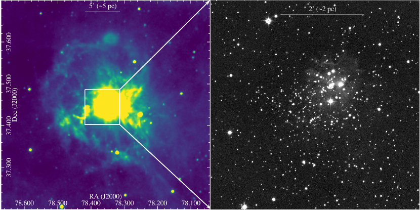
Figure 1: The left panel displays the WISE 12 $\mu$m image dust distribution around the cluster having an area of 30$\times$30  arcmin², while the right panel displays the UKDISS $H$-band image of the central 5$\times$5  arcmin² area.

It is believed that most, if not all, stars form in embedded clusters (Lada & Lada, 2003). In general, parsec-scale young clusters (age $>$ 2 Myr) have smooth, centrally condensed and nearly spherical structure (Ascenso et al., 2007; Harayama et al., 2008), while molecular clouds, in general, have irregular and much extended (up to tens of parsecs) structure (André et al., 2008; Molinari et al., 2010). In this context, a key question is “How centrally condensed clusters form from such molecular clouds?” Although, there are various proposed mechanisms of cluster formation such as the monolithic collapse of molecular clouds, hierarchical collapse and merger of gas and star(s), and global non-isotropic collapse (Longmore et al., 2014; Banerjee & Kroupa, 2015; Motte et al., 2018; Vázquez-Semadeni et al., 2019), yet it is unclear that which process plays a dominant role under which circumstances. Moreover, it is not known if other dynamical processes such as two-body relaxation and mass-segregation are also responsible to shape the structure of the newly born clusters (Banerjee & Kroupa, 2017; Sills et al., 2018). These questions can be addressed by studying young clusters while they are still associated with gas and dust. Another key question related to cluster formation, in particular associated with the formation of massive to intermediate-mass clusters, is whether such clusters play a constructive or destructive role in the future star formation processes of the host cloud. Because massive members of such clusters, on one hand, can switch off the star formation by blowing off the gas and dust from their immediate vicinity, while on the other hand, they can compress the cold parental gas to promote the star formation (Elmegreen & Lada, 1977; Deharveng et al., 2010) in the cloud. And the latter can prolong the star formation activity of a molecular cloud up to several million years (e.g. Preibisch & Mamajek, 2008). In the past, studying the early evolution of young clusters had been an observational challenge as they are buried inside molecular clouds. Recent sensitive surveys over the last decade, however, have provided a wealth of data in optical to mm domain (e.g. Jackson et al., 2006; Lawrence et al., 2007; Minniti et al., 2010; Molinari et al., 2010; Chambers et al., 2016; Gaia Collaboration et al., 2016). These surveys allow us to better understand the properties of the young clusters, and characterize the physical conditions of the surrounding interstellar medium (ISM). For example, by using parallax and proper motion (PM) measurements obtained from the Gaia (Gaia Collaboration et al., 2016, 2018) survey data, distance to the star clusters can precisely be estimated (Bailer-Jones et al., 2018) and membership of the bright stars can be well constrained. Similarly, using deep infrared data sets from surveys such as UKIDSS (UKIRT Infrared Deep Sky Survey) Galactic Plane Survey (UKIDSS-GPS; Lucas et al., 2008), Spitzer Galactic Legacy Infrared Mid-Plane Survey Extraordinaire (GLIMPSE; Whitney & GLIMPSE360 Team, 2009) survey and Wide-field Infrared Survey Explorer (WISE; Wright et al., 2010) pre-main-sequence (PMS) members of the young clusters can be identified (e.g. Gutermuth et al., 2009; Das et al., 2021). Moreover, for moderately extincted nearby clusters, age determination is possible by constructing color-magnitude diagrams (CMD) using data from optical surveys such as the $Gaia$ (Gaia Collaboration et al., 2018), the Panoramic Survey Telescope and Rapid Response System (Pan-STARRS1; Chambers et al., 2016) and Sloan Digital Sky Survey (SDSS; Alam et al., 2015). In addition to that, using wide area maps provided by surveys such as Herschel infrared Galactic Plane Survey (Hi-GAL Pilbratt et al., 2010; Molinari et al., 2010) and FCRAO (Five College Radio Astronomical Observatory; Jackson et al., 2006), connections between large-scale environment and the cluster forming clumps can be made.

In the present work, we characterize the young cluster IRAS 05100+3723 (Bica et al., 2003) associated with the H ii region Sharpless 228 (hereafter S228, Sharpless, 1959), also known as LBN 784, and RAFGL 5137 ($\alpha_{2000}$=78.^∘356250, $\delta_{2000}$=+37.^∘450278). The H ii region is believed to be powered by a massive star ALS 19710 of spectral type between O8V to B0V, whose reddening ($E(B-V)$), lies in the range 1.2$-$1.3 mag (Chini & Wink, 1984; Hunter & Massey, 1990). We study the physical conditions of dust and gas around the cluster by taking advantage of the key strengths of the aforementioned multiwavelength surveys. Figure 1 shows the WISE 12 $\mu$m image around the cluster over 30$\times$30 arcmin² area as well as the central 5$\times$5 arcmin² area in the near-infrared (NIR) $H$-band from the UKIDSS-GPS (Lucas et al., 2008) wherein the cluster is clearly visible. There are several shallow optical and infrared studies on the cluster suggesting that the cluster is located at a distance between 2.2 and 6.8 kpc and its age lies somewhere between 1 and 25 Myr (Lahulla, 1985; Hunter & Massey, 1990; Kharchenko et al., 2013; Yu et al., 2018). To date, the most detailed work on the cluster has been carried out by Borissova et al. (2003) using NIR observations. Their results suggest that the age of the cluster is $\sim$3 Myr and its total stellar mass is $\sim$1800  M_☉. This makes the cluster one of the potential young massive clusters in our Galaxy such as Orion Nebula Cluster (ONC, mass $\sim$2000 M_☉  and age $\sim$3 Myr, see Hillenbrand, 1997; Da Rio et al., 2010), albeit at a farther distance. Borissova et al. (2003) estimated the cluster radius to be 1.5 arcmin  while Yu et al. (2018) reported the cluster radius to be 2.5 arcmin.

Intermediate-mass to massive young clusters are rare in our Galaxy. For example, Lada & Lada (2003), in their study of young ($<$ 3 Myr) embedded clusters within 2 kpc of the solar neighborhood, found that the only cluster that has stellar mass $>$ 1000 M_☉  is the ONC. Thus, a cluster like IRAS 05100+3723 serves as a potential candidate for understanding the formation and early evolution of intermediate-mass to massive clusters. Despite the fact that IRAS 05100+3723 is a potentially young massive cluster, its detailed stellar content, physical properties, and surrounding ISM are scarcely explored. In this work, we examine the stellar, gaseous, and dust components of this likely massive cluster and its environment, with the aim to understand its formation history and feedback effects on the star formation processes of the host cloud.

We organize this paper as follows. In Section 2 we present the observations, archival data sets and data reduction procedures. Section 3 discusses the stellar content and properties of the cluster, and the physical conditions and kinematics of the large-scale environment. Section 4 discusses the dynamical status of the cluster, its formation history, and the effect of stellar feedback on the star formation scenario of the complex, followed by a summary in Section 5.

2 Observations and Data Sets

2.1 Optical Spectroscopic Observations

We obtained medium-resolution spectra for three bright stars in the S228 complex using the Medium Resolution Spectrograph (MRES) mounted on the 2.4 m Thai National Telescope (TNT). The MRES is a fiber-fed echelle spectrograph designed to work in spectral range of  3900$-$8800Å  with a spectral resolution of R $\sim$16,000$-$19,000. This instrument is equipped with a 2048$\times$512 pixels Andor CCD camera with a pixel size of 13.5 $\mu$m.

The data were acquired on the night of 2019 March 18 with a lunar illumination of $\sim$80% during partially cloudy weather conditions. The log of the observations is given in Table 1. In addition to the science spectra, we obtained standard calibration frames such as Bias, Flat and Th-Ar lamp. The data reduction was carried out using the echelle standard package of IRAF. The spectra were extracted using optimal extraction methods. The wavelength calibration of the spectra was done using Th-Ar lamp source. The wavelength calibrated, normalized spectra of the three stars are shown in Figure 2. We discuss the spectral classification of these stars in Section 3.1.1. It should be noted that only a part of the spectra, i.e. in the range 4400$-$6800 Å,  is being used in this work. The spectra in the range 3900$-$4400 Å  are dominated by noise due to poor sensitivity in this range and spectra beyond 6800 Å  are dominated by multiple telluric lines/bands and hence not used in our analysis.

Table 1: Log of the MRES observations.

ID	$\alpha_{2000}$	$\delta_{2000}$	Date of	V	Exposure
	(∘)	(∘)	observation	(mag)	time (sec)
1	078.356250	+37.458222	2019-03-18	12.6	2,700
2	078.356667	+37.458167	2019-03-18	13.2	3,000
3	078.353333	+37.453250	2019-03-18	13.1	3,000

2.2 Radio Continuum Observations

Radio continuum observations of the S228 region were obtained at 610 and 1280 MHz using the GMRT array (PI: M.R. Samal, ID: 13MRS01) with the aim to trace the ionized gas content of the cluster. The GMRT array consists of 30 antennae arranged in an approximate Y-shaped configuration, with each antenna having a diameter of 45 m. Details about the GMRT can be found in Swarup et al. (1991).

The Very Large Array (VLA) phase and flux calibrators ‘0555+398’ and ‘3C48’, respectively, were used for these observations. We carried out the data reduction using the aips software and followed the procedure described in Mallick et al. (2013). Briefly, we used various aips tasks for flagging the bad data and calibrating the data with standard phase and flux calibrators. Thereafter, we run the aips task ‘IMAGR’ to make maps after splitting the source data from the whole observations. We applied a few iterations of (phase) self-calibration to remove ionospheric phase distortion effects. The resultant maps are discussed in Section 3.2.1.

2.3 Ancillary Archival Data Sets

For the present work, we have also used the following archival data sets covering various wavelengths:

i) $Gaia$ Early Data Release 3 ($Gaia$ EDR3 Gaia Collaboration et al., 2020) from the European Space Agency Gaia mission (Gaia Collaboration et al., 2016). We used the kinematic information of Gaia data to estimate the distance to the cluster. The effective angular resolution of the survey is $\sim$0.4 arcsec.

ii) The Spitzer-IRAC warm mission data at 3.6 and 4.5 $\mu$m data (PI: Barbara Whitney, Program ID: 61070) from the $Spitzer$ Heritage Archive (SHA). We acquired the corrected basic calibrated data (cbcd), uncertainty (cbunc), and imask (bimsk) files. In order to create the final mosaic images with a pixel scale of 1.2 arcsec  pixel^-1, and to obtain the aperture photometry of the point sources, we followed the steps mentioned in Yadav et al. (2016) and used sources with uncertainty $<$ 0.2 mag for our analysis.

iii) The NIR ($J,H,$ and $K$) photometric data, from the UKIDSS-GPS (Lucas et al., 2008), with uncertainty $<$ 0.2 mag in all three bands. The spatial resolution of the UKIDSS-GPS data is in the range 0.8$-$1 arcsec.

iv) The INT/WFC Photometric H$\alpha$ Survey of the Northern Galactic Plane (IPHAS) data release 2 (Barentsen et al., 2014) photometric data with uncertainty $<$ 0.2 mag in Sloan $r$, $i$ broad-band and H$\alpha$ narrow-band filters. The spatial resolution of the IPHAS data is in the range 0.8$-$1 arcsec.

v) The Pan-STARRS1 (hereafter; PS1 Chambers et al., 2016) survey photometric data with uncertainty $<$ 0.2 mag in $i_{\rm{P1}}$  and $z_{\rm{P1}}$  bands were used to estimate the age of the cluster. The spatial resolution of the PS1 data is in the range 0.8$-$1 arcsec.

vi) The far-infrared images from the Herschel infrared Galactic Plane Survey (Hi-GAL) (Molinari et al., 2010) images at 70, 160, 250, 350, and 500 $\mu$m were used. The spatial resolution of the Hi-Gal observation at 70, 160, 250, 350, and 500 $\mu$m bands is 8.5, 13.5, 18.2, 24.9, and 36.3 arcsec, respectively.

vii) The radio continuum image at 8700 from the National Radio Astronomy Observatory (NRAO) data archive (Project ID: AR390). The beam size of the image is $\sim$10 arcsec$\times$ 8 arcsec while its rms noise is $\sim$0.1 $\mu$Jy beam^-1.

viii) The radio continuum image at 150 MHz from the TIFR GMRT Sky Survey (TGSS) (Intema et al., 2017). The typical resolution of the TGSS images is $\sim$25 arcsec$\times$25 arcsec  with a median noise of $\sim$3.5 mJy beam^-1.

2.3.1 Completeness of Photometric Data

In this work, we used UKDISS, Spitzer-IRAC and IPHAS data sets to access the young stellar contents of the cluster. We obtained the completeness limits of these bands using the histogram turnover method. Although this method is not a formal tool to measure the completeness, it serves as a proxy to give the typical value of completeness limit across the field (e.g. Samal et al., 2015; Damian et al., 2021). In this approach, the magnitude at which the histogram deviates from the linear distribution is, in general, considered as 90% complete. Figure 3 shows histograms of sources detected in various bands over a radius $\sim$2.5′(see Section 1). The above approach suggest, in general, our photometry is $\sim$90% complete down to $J$ = 17.8 mag, $H$ = 16.8 mag, $K$ = 16.2 mag and [4.5] = 15.5 mag, these are marked by vertical lines in Figure 3. Similarly, we also estimated the completeness limits of IPHAS $r$, H$\alpha$ , and $i$; and PS1 $i_{\rm{P1}}$  and $z_{\rm{P1}}$  bands as 20.3 mag, 19.8 mag, and 19.0 mag; and 20.4, and 19.7 mag, respectively.

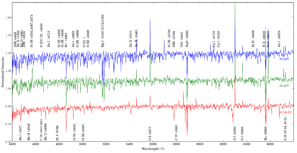
Figure 2: Continuum normalized and scaled spectra of three bright stars #1, #2, and #3 observed with MRES mounted on TNT. Important stellar lines are marked.

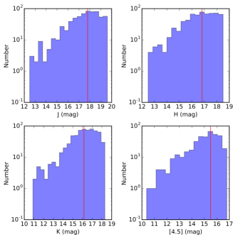
Figure 3: Histograms of the sources detected in $J,H,K$, and [4.5] $\mu$m photometric bands. The vertical red lines indicate the 90% completeness limit. See the text for details.

3 Analysis and Results

3.1 Stellar Content and Properties of the Cluster

In this section, we access massive and low-mass stellar contents of the cluster and derive cluster properties using various photometric catalogs.

3.1.1 Spectral Classification and Modeling of the Bright Sources

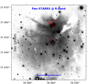
Figure 4: Pan-STARRS $r$-band image of the cluster along with the sources for which spectroscopic observations have been conducted. The ID and the coordinates of the sources are given in Table 1.

The cluster IRAS 05100+3723 is associated to an H ii region, implying that its massive members must be responsible for the ionization of the region. To identify the ionizing source(s) of the H ii region, we selected three bright sources located within the region of strong H$\alpha$ emission. Following Comerón & Pasquali (2005), we use the infrared reddening-free pseudo color index, Q = ($J-H$) $-$ 1.70$\times$($H-K$) and select sources with Q $<$ 0.1 as probable OB stars of the region. These sources are marked in Figure 4 as #1, #2, and #3. However, selected sources may be contaminated by objects such as AGB stars, carbon stars, and A-type giants (Comerón & Pasquali, 2005). We thus performed optical spectroscopic analyses of these three bright sources.

As mentioned in Section 2.1, observations were carried out under the cloudy weather conditions during the waxing Moon with  80% illumination. This caused the stellar spectra to be heavily contaminated with the solar lines. The contamination becomes more obvious upon close examination of the spectra  (Figures 2, and 5). The variable contamination of stellar spectra restricts our capabilities to find the accurate physical parameters of the stars, but the spectra still contain enough markers of the effective temperature.

The abundance of neutral and/or ionized helium lines in absorption is indicative of O or early B type main sequence stars. These lines may be in emission in case of giants/super giants. The strength of He ii 4686 gets weaker for late O-type stars, and this line is last seen in B0.5 stars (Walborn & Fitzpatrick, 1990). We could find such lines only in the spectrum of the star #1. To further constrain this, we compare our data with synthetic spectra computed for different combinations of effective temperature, surface gravity, and projected rotational velocity. Theoretical spectra were synthesized with Synplot, an IDL-based wrapper of the Synspec package for spectral synthesis (Hubeny & Lanz, 2011). We use “OSTAR2002” grid of pre-computed models of  Lanz & Hubeny (2003).

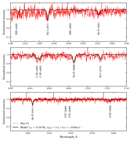
Figure 5: Part of the MRES spectrum (red) for the source #1 fitted with a synthetic profile (black). The synthetic spectrum was computed using the parameters specified in the text.

In the observed spectrum, we identified multiple neutral and ionized helium, carbon, and oxygen lines (Figure 5). Among them, two helium lines He I $\lambda 4471$ and He II $\lambda 4541$ are good indicators of effective temperature. The intensity ratio of these lines equals to 1 for the spectral class O7 (Walborn & Fitzpatrick, 1990) and it varies between $>$ 1 and $<1$ for the spectral range O5$-$O9. This intensity ratio for star #1 is estimated to be $<1$. By fitting synthetic spectrum, we derive the effective temperature $T_{eff}=33,000\pm 1000$ K and surface gravity $\log g=3.8\pm 0.5$ (Figure 5), which allowed us to classify this object as an O8.5V$\pm$0.5 star. The synthetic spectrum was computed for $T_{eff}=33,000\pm 1000$ K, $\log g=3.8\pm 0.5$, and $v\sin i=100\pm 50$ km/s for the whole wavelength range, which agrees well with the observed lines in other spectral regions and thereby verifies our estimates.

The spectral types of the two fainter stars are less certain. Their spectra do not contain any measurable lines of helium, which are typical of OB stars. Instead, from the comparison with the solar spectrum we identified neutral iron, chromium and titanium (see Figure 2) lines. Detailed modelling of these spectra was carried out using the NEMO grids of stellar atmospheres computed with a modified version of the ATLAS9 code (Heiter et al., 2002). The modelling results show that the star #2 is hotter than the Sun and has an effective temperature $7000\pm 1000$ K whereas the star #3 looks comparatively cooler with a probable effective temperature of 6400 K. The existing data do not allow us to determine the surface gravity (and thus the evolutionary status) of these stars with higher accuracy. Our spectral analysis suggests that stars #2 and #3 are late A to F type stars. Indeed, the Gaia data confirmed that stars #2 and #3 are the foreground objects, as discussed in Section 3.1.3.

3.1.2 Physical Extent

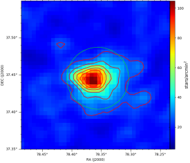
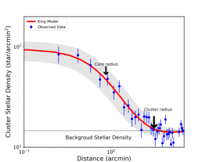
Figure 6: Upper Panel: Stellar surface density map of S228, made using the nearest neighbors method. The color bar represents the stellar surface density in the units of stars per arcmin². Contours correspond to stellar surface densities above $3\sigma$ of the mean background density, where $\sigma$ is the standard deviation of the background density. The green circle represents the cluster region whose radius was obtained using the radial density profile fitting method shown in the lower panel. Lower Panel: The observed stellar surface density (filled circles) of S228 as a function of radius. The horizontal line represents the mean density level of the field stars. The continuous curve shows the fitted King’s profile to the observed data, while the shaded area represents the $1\sigma$ error associated to the fitted profile. The error bars represent the Poisson uncertainties.

We derived the physical extent of the cluster by generating the stellar surface density map (SSDM) using UKDISS point sources. In order to generate the SSDM map, we use the nearest neighbors algorithm as described in Gutermuth et al. (2005). Succinctly, at each sample position [$i,j$] in a uniform grid, we measured $r_{N}$($i,j$), the projected radial distance to the $N^{th}$ nearest star. $N$ is allowed to vary to the desired smallest scale structures of interest. We generated the map using $N$=20, which, after a series of tests, was found to be a good compromise between the resolution and signal-to-noise ratio of the map. The resultant map is shown in Figure 6 (upper panel) along with stellar surface density contours. We then considered the peak (at $\alpha_{2000}$= 78.^∘366083 $\delta_{2000}$= +37.^∘444889) of the SSDM map as the cluster center.

We also constructed a radial density profile (RDP) of the cluster. The RDP is generated by plotting the annular stellar density against the corresponding radius (for details, see Panwar et al. (2019)). In order to parametrize the RDP, the observed RDP is fitted with the empirical King’s profile (King, 1962), which is of the form:

$$\rho(r)\propto b_{0}+\frac{\rho_{0}}{\left(1+\left(\frac{r}{r_{c}}\right)^{2}\right)}$$ (1)

where b₀, $\rho_{0}$ and $r_{c}$ are the background stellar density, peak density, and core radius, respectively. The fitted King’s profile, shown in the lower panel of Figure 6, yields a central density of $\rho_{0}$ = 116 stars arcmin^-2, a core radius of $r_{c}$ = 0.8 arcmin  and a background density $b_{0}$ = 13 stars arcmin^-2. From Figure 6, we note that the model profile merges with the background density at 2.5 arcmin and is almost constant beyond the radius of $\sim$3.0 arcmin. We thus considered the radius of the cluster to be 2.5 arcmin. The estimated radius is in agreement with the cluster size of 5.2 arcmin  (or radius of 2.6 arcmin) reported in Yu et al. (2018). A circle of thus estimated radius is also over plotted on the SSDM, which is in good agreement with the size of the SSDM map.

3.1.3 Distance

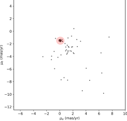
Figure 7: Proper-motion vector diagram (PVD) for all the sources toward S228 within the cluster region. Sources distributed in the red zone represent the likely cluster members.

The distance of S228 is quite uncertain, ranging from 2.2 to 6.8 kpc (Lahulla, 1985; Hunter & Massey, 1990; Borissova et al., 2003; Balser et al., 2011; Kharchenko et al., 2013). With the aim to tighten the distance of the cluster, we searched for the kinematic members of the cluster using the Gaia EDR3 catalog. Figure 7 shows the proper-motion vector diagram (PVD) of relatively bright sources ($G$ $<$ 18 mag) within the cluster radius. As can be seen, there are two likely distributions in the PVD, i) a compact group consisting of sources of similar motion (marked with red zone), thus are considered as cluster members, and ii) a loose group of sources showing scattered motion, thus are considered as field sources. A clear separation between the cluster and field stars motion enables us to select member stars of S228 relatively reliably. Among the compact group sources, we reject a few outliers, by keeping only those sources whose parallax ($\varpi$) values are within one standard deviation of the median parallax of the group and have good relative parallax uncertainties ($\varpi$/$\sigma_{\varpi}$ $>$ 5). The latter condition is primarily motivated by the fact that, if fractional parallax errors are less than about 20%, then the posterior probability distribution of parallax is nearly symmetric (Bailer-Jones, 2015), hence, distance can simply be computed by inverting the parallax. With these constraints, 7 sources are found to have common proper motions (PM) and parallaxes. We find that among these sources, the ionizing source (i.e. star #1) is one of the members, while the other bright spectroscopic sources (i.e. star #2 and #3) are not members, confirming our spectroscopic membership. The PM in Right Ascension ($\mu_{\alpha}$), PM in Declination ($\mu_{\delta}$) and parallax ($\varpi$) values of these sources lie in the range $-0.10$ to 0.37 mas yr^-1, $-1.45$ to $-1.30$ mas yr^-1 and 0.28 to 0.39 mas, respectively, with median -0.01 $\pm$ 0.15 mas yr^-1, $-$1.40 $\pm$ 0.06 mas yr^-1, and 0.31 $\pm$ 0.04 mas. From the median parallax value, we estimated the distance of the cluster to be 3.2 $\pm$ 0.4 kpc, which is in agreement with the kinematic distance of 3.5 kpc, very recently derived by Mège et al. (2021) using velocity analysis of the molecular gas associated to the region.

3.1.4 Pre-Main-Sequence Members

In the absence of spectroscopic or kinematic information of low-mass sources, optical and infrared color-color (CC) diagrams are often used as diagnostic tools to identify the likely PMS members in a star-forming region (e.g. Lada & Adams, 1992; Barentsen et al., 2011). In this work, we used IPHAS, UKIDSS-GPS, and Spitzer-IRAC point source catalogs above the completeness levels and employed CC diagrams to search for the PMS stars with either excess NIR emission due to the presence of circumstellar disc or excess H$\alpha$ emission due to accretion onto the stellar photosphere. The details about the CC diagrams and the identified sources are given below.

H$\alpha$ Excess Emission Sources

The ($r-$H$\alpha$ ) color measures the strength of the H$\alpha$ line relative to the $r-$band photospheric continuum. Since most main-sequence stars do not show H$\alpha$ emission, their ($r-$H$\alpha$ ) color, which is linked to spectral type, provides a template, against those whose ($r-$H$\alpha$ ) color excess caused by H$\alpha$ emission. Moreover, in the ($r-$H$\alpha$ , $r-i$) CC space, interstellar reddening has minimal effect on ($r-$H$\alpha$ ) color as the reddening moves only the unreddened MS track almost with a right angle to the ($r-$H$\alpha$ ) color. Thus, in star-forming complexes, the ($r-$H$\alpha$ , $r-i$) diagram is often used to discern H$\alpha$ emission line stars (Barentsen et al., 2011; Dutta et al., 2015). The ($r-$H$\alpha$ , $r-i$) CC diagram for the stars in the direction of S228 is shown in Figure 8. The running average ($r-$H$\alpha$ ) color of the stars as a function of their ($r-i$) color is shown with a solid line, while its 10$\sigma$ uncertainty is shown with a shaded area. Figure 8 shows the ($r-$H$\alpha$ , $r-i$) color of the main-sequence (MS) track taken from Drew et al. (2005) for $A_{\it V}$ $\sim$3.1 mag. Using this diagram, those sources with ($r-$H$\alpha$ ) color excess greater than 10$\sigma$ of the average color of the stars are considered as probable emission line sources, and are marked with red circles. With this approach, we identified 21 likely H$\alpha$ excess sources.

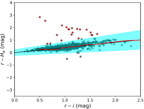
Figure 8: The IPHAS CC ($r-$ H$\alpha$ , $r-i$) diagram of the point sources in the direction of the cluster. The median ($r-$H$\alpha$ ) color of the field sources and 10$\sigma$ limits around the median color line (blue) is shown with a shaded area. The red curve represents the synthetic MS track taken from Drew et al. (2005) corresponding to E(B-V) = 1.0 mag (or $A_{\it V}$ $\sim$3.1 mag). The filled red circles are the probable H$\alpha$ excess candidates within the cluster area.

Near-Infrared Excess Emission Sources

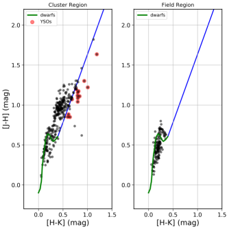
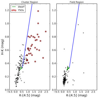
Figure 9: Left: The ($J-H$, $H-K$) CC diagram for the cluster region and the control field region. The green curves are the intrinsic dwarf locus from Bessell & Brett (1988). Right: The ($H-K$, $K-$ [4.5]) CC diagram for the cluster region and the control field region. The green curves are the intrinsic dwarf locus of late M-type dwarfs (Patten et al., 2006). In all the plots, the blue lines represent the reddening vectors drawn from the location of M6 dwarf, while the red circles represent likely NIR$-$excess sources.

The NIR ($J-H$, $H-K$) diagram is a useful tool to identify PMS sources exhibiting NIR$-$excess emission. However, other dusty objects along the line of sight may also appear as NIR$-$excess sources in the CC diagram. One possible way to separate out PMS sources is to compare the CC diagram of the cluster with that of a nearby control field of the same area and photometric depth. The left panel of Figure 9 shows NIR CC diagrams of the cluster as well as a control field (centered at $\alpha_{2000}$= 78.^∘382386, $\delta_{2000}$= 37.^∘17977) located $\sim$5 arcmin away from the cluster field. In the NIR CC diagram, sources distributed left to the reddening vector (blue line) can be field stars or reddened MS stars or weak-line T$-$Tauri stars, while sources located right to the reddening vector are considered as PMS sources with NIR$-$excess (Lada & Adams, 1992). As can be seen in Figure 9, compared to the cluster region, the NIR$-$excess zone of the control field is devoid of sources, implying the presence of true NIR$-$excess sources in the cluster region. However, in order to separate spurious sources, if any, from genuine excess sources we selected sources based on the following criteria: i) sources with ($J-H$) color greater than 0.7 mag because the maximum ($J-H$) color of the control field population is around 0.7 mag, and ii) sources that fall to the right of the reddening vector with ($H-K$) color excess larger than the uncertainties in their respective ($H-K$) colors. With this approach, we identified 14 NIR-excess candidate sources within the cluster region. These sources are identified as red circles in Figure 9.

It is well known that circumstellar emission from young stars dominates at longer wavelengths, where the spectral energy distribution (SED) significantly deviates from the pure photospheric emission. We thus use Spitzer-IRAC observations in combination with $JHK$ data to identify additional NIR$-$excess sources. For this purpose, we use the ($H-K$, $K-$[4.5]) CC diagram, shown in the right panel of Figure 9. It should be noted that we preferred 4.5 $\mu$m data over 3.6 $\mu$m as it is less affected by Polycyclic aromatic hydrocarbon (PAH) emission, which is often present in the H ii region environments (Smith et al., 2010). Similar to ($J-H$, $H-K$) analysis, we compared the distribution of cluster sources with control field sources, then selected NIR$-$excess sources whose excess emission is more by the error associated to the $K-[4.5]$ color of the sources and ($H-K$) color greater than 0.4 mag. With this approach, we identified 25 additional candidate stars with NIR excess. This makes 39 NIR excess sources in total.

In summary, with the above approaches, we identified 21 likely H$\alpha$ emission line sources and 39 NIR excess sources. Among 21 H$\alpha$ sources, 6 sources are found to have NIR excess counterparts. In total, within the cluster region, we identified 54 PMS sources. Out of the 54 PMS sources, 52 sources have optical counterparts in the Pan-STARRS1 bands, and are used to derive the age of the cluster.

3.1.5 Extinction

We derived visual extinction of the cluster using its likely OB members. Briefly, we select OB stars from the Gaia member sources (e.g, see Samal et al., 2010) identified in Section 3.1.3 by considering only those sources whose Q value is $<$ 0.1 showing no NIR excess. This resulted in five sources out of the seven Gaia members. We then derived the ($H-K$) color excess, $E(H-K)$, of the members from the observed and intrinsic ($H-K$) colors. Since the most massive star of the cluster is an O8.5V star, we thus adopted an intrinsic ($H-K$) color of $\sim$0.03 mag for our analysis, which is the mean intrinsic color of O8 to B9 MS stars as tabulated in Pecaut & Mamajek (2013). We then estimated the visual extinction of the sources using the relation, $A_{V}$ = 15.9 $\times$ $E(H-K)$, adopting the extinction laws of Rieke & Lebofsky (1985). This yields a mean visual extinction $A_{\it V}$ = 3.3 $\pm$ 0.6 mag, which is in agreement with the extinction measurements between 3.0 mag (Lahulla, 1985) and 3.9 mag (Hunter & Massey, 1990) derived for S228.

3.1.6 Age

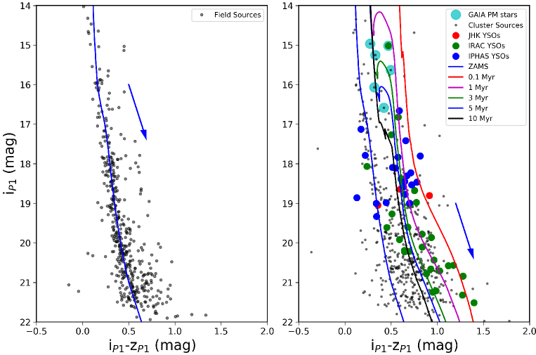
Figure 10: The optical ($i_{\rm{P1}}$, [$i_{\rm{P1}}$- $z_{\rm{P1}}$]) CMD of the control field (left panel) and cluster region (right panel). In the cluster CMD, the NIR$-$excess sources identified based on $JHK$ and $HK[4.5]$ bands are shown by red and green circles, while the H$\alpha$ excess sources are shown by blue circles, and the PM based massive members are shown by cyan circles. In cluster CMD the PMS isochrones of ages 0.1, 1, 3, 5, 7 and 10 Myr from Dotter (2016) are shown from left to right, while the blue solid curves in both the CMDs represent the ZAMS isochrone, to guide the distribution of filed stars in both the plots. All the PMS isochrones are corrected for a distance of 3.2 kpc and an average reddening of $A_{\it V}$ = 3.3 mag. In both the plots, the reddening vectors corresponding $A_{\it V}$ =0.5 mag are shown by slanted arrows.

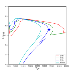
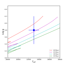
Figure 11: The (gravity ($g$), temperature ($T_{eff}$)) diagrams for the massive star. In the upper panel, the thin solid curves are the MESA isochrones for ages 2, 4, 6, and 10 Myr, while in the lower panel the dashed lines are the evolutionary tracks for 20, 25, 30 and 35 M_☉.

The ages of young clusters are typically derived by fitting theoretical PMS isochrones to the low-mass contracting population. To derive the age of IRAS 05100+3723, we use optical ($i_{\rm{P1}}$, [$i_{\rm{P1}}$$-$$z_{\rm{P1}}$]) CMD of the PMS sources identified in Section 3.1.4 as the cluster members. We chose $i_{\rm{P1}}$  and $z_{\rm{P1}}$  bands to derive the age, as both of these bands have higher PMS counterparts over other bands of the PS1 survey. Moreover, benefits of using optical bands are that i) it minimizes the effect of the excess emission compared to NIR bands, and ii) it minimizes the effect of differential reddening as the reddening vectors are nearly parallel to the isochrones. Figure 10 shows the ($i_{\rm{P1}}$, [$i_{\rm{P1}}$$-$$z_{\rm{P1}}$]) CMDs of the cluster (right) as well as the nearby control field (left). In the cluster CMD, all the sources within the cluster area and the likely PMS sources are shown with grey dots and filled circles, respectively. We find that the average $A_{\it V}$ of the control field population is likely around 2.3 mag, which is estimated by matching a reddened theoretical "zero-age main sequence" (ZAMS) with the observed population. To guide our analysis, we have also plotted ZAMS at $A_{\it V}$ = 2.3 mag on the cluster CMD. A careful comparison of the distribution of the PMS sources and the control field sources on the CMD reveals that the majority of the PMS sources are redder compared to the ZAMS isochrone at $A_{\it V}$ = 2.3 mag. Comparison of both the diagrams reveals that the field population is quite significant in the direction of the cluster.

Next, we over-plotted MESA (Modules for Experiments in Stellar Astrophysics) isochrones (Dotter, 2016) on the CMD after correcting them for the adopted distance of 3.2 kpc and extinction of $A_{\it V}$ = 3.3 mag. The adopted extinction value is also found to match well with the bright PM based cluster members, implying that for the cluster, the average $A_{\it V}$ = 3.3 mag is a reasonable assumption. We note that compared to the field population, the extra extinction of $A_{\it V}$ = 1 mag observed in the direction of the cluster could be intrinsic to the cluster. In fact, we find that the cluster is still associated with gas and dust as seen in Figure 22 supporting the above hypothesis. As can be seen from Figure 10 the location of most of the PMS sources are in the age range 0.1$-$10 Myr, implying that the cluster is young. We note that a small fraction of H$\alpha$ emitting sources are found to be close to the field distribution. Such sources could be contaminants such as carbon stars, white dwarfs, and/or interacting binaries (for details, see Barentsen et al., 2011). In this analysis, we consider all the PMS sources younger than 10 Myr as most likely cluster members, because the level of accretion activity for PMS sources older than 10 Myr is expected to be very low (Williams & Cieza, 2011). Then we derive the age of the individual PMS sources by comparing their location with isochrones having age between 1 and 10 Myr with an interval of 0.1 Myr. We assign PMS sources an age equal to the age of the closest isochrone. In this process, some sources located to the right of the 0.1 Myr isochrone are simply considered to have an age of 0.1 Myr. Doing so, we estimate the mean age of the PMS sources, thus of the cluster, to be $\sim$2.1 $\pm$ 1.3 Myr. Although the smaller sample of PMS sources and variable extinction limit us to derive a very precise age of the cluster, yet it agrees well with the age estimates of Borissova et al. (2003).

To ascertain our result, we further use the properties of the massive star derived in Section 3.1.1. To do so, we compared the derived $T_{eff}$ and log $g$ of the star with the MESA isochrones and stellar evolutionary tracks as shown in Figure 11. As can be seen, because of a large error in log $g$ value, the location of the star in Figure 11 spans over a wide range of mass and age. Although accurate stellar parameters are needed to constrain the age of the star more precisely, nonetheless, we use the Bayesian approach implemented in the isochrones package (Morton, 2015) to derive the most probable age and mass of the star. The isochrones package uses the nested sampling scheme MULTINEST (Feroz et al., 2009) to capture the true multi-modal nature of the posteriors. Figure 12 shows the obtained posterior probability confidence contours of mass and age with the Bayesian approach. The peak of the likelihood distribution is considered as the most probable value, and the estimated uncertainty is determined by considering 15 and 85 percentile values of the likelihood distribution. With this approach, we find the most probable age of the star to be $\sim$4 Myr, while the most probable mass to be $\sim$20 M_☉. If one takes the average uncertainty associated to the most probable value, then the age, 4.0 $\pm$ 2.7 Myr, is in reasonable agreement with the age, 2.1 $\pm$ 1.3 Myr, derived using CMD of the low-mass stars.

With these two approaches, the average age turns out to be 3.0 $\pm$ 1.5 Myr, which we considered as the age of the cluster for further analyses. Since the cluster is associated with an H ii region that is still bright in optical and radio bands, thus one would expect the cluster to be young. Our analysis confirms this hypothesis.

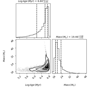
Figure 12: The lower-left plot shows the posterior probability distributions of mass and age of the massive star obtained from the isochrone fitting. The upper-left and lower-right plots are the probability distribution histograms for the mass and age, respectively. The middle line in the histogram plots is the median value of the distribution, while the left and right lines represent the 16% and 84% percentile values, respectively.

3.1.7 Mass Function and Total Stellar Mass

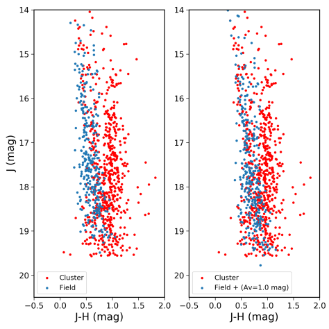
Figure 13: The ($J$, $J-H$) CMDs of the cluster (red dots) and the control field (blue dots). In the left panel, control field sources are plotted without any reddening correction, while in the right panel an extra reddening corresponding to $A_{\it V}$ = 1.0 mag have been applied to control field sources.

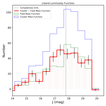
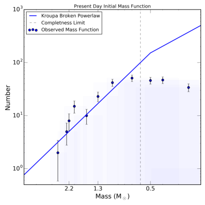
Figure 14: Left Panel: The green and blue histograms represent the $J$-band luminosity functions of the cluster and control fields, respectively, while the luminosity function after correcting for the field-star contamination is shown with the red histogram. The control field is reddened by $A_{\it V}$ = 1 mag. In the plot, the vertical dashed line represents the $\sim$90% completeness limit of the $J$-band, while the error bars represent the Poisson uncertainties. Right Panel: Present-day mass function of the cluster computed from the field-star decontaminated $J$-band luminosity function and is shown by dots. The 90% mass completeness limit of the data in terms of mass is shown by a vertical dashed line. The fitted power law of the observed mass function is shown by a blue line and is extended towards the low-mass end using the functional form of the mass function given by Kroupa (2001).

The stellar initial mass function (IMF) describes the mass distribution of the stars in a stellar system during birth and is fundamental to several astrophysical concepts. For a young cluster, IMF is in general derived from the luminosity function of member stars above the completeness limit. In our case, adopting the estimated age and extinction of the cluster, we find the photometric completeness limits of our $J,H,$ and $K$ bands (see Section 2.3) correspond to mass completeness limits of 0.6 M_☉, 0.6 M_☉, and 0.7 M_☉, respectively. We then used the $J$-band luminosity function (JLF) to derive the IMF. The selection of the $J$-band is motivated mainly by the fact that the effect of circumstellar excess emission in the $J$-band is minimum compared to the $H$ and $K$ bands (see Section 2.3.1), and moreover its mass sensitivity is comparable to these bands. Figure 13 (left panel) shows the ($J$, $J-H$) CMD for the cluster as well as the control field. As can be seen from the figure, the cluster region (red dots) appears to have bi-modal color distributions, in which a group of redder sources with $J$ $>$ 16.0 mag are relatively well separated from a group of bluer sources. This implies that the redder sources are likely the cluster members, while the bluer sources are likely the field population in the direction of the cluster. One may also notice that compared to the ($i_{\rm{P1}}$, [$i_{\rm{P1}}$- $z_{\rm{P1}}$]) CMD shown in Fig. 10, the ($J,J-H$) CMD shows a richer population of young sources. This could be due to the fact that infrared bands are less affected by extinction, and also young sources are intrinsically bright at longer wave bands. In the present case, we have detected 112 extra sources in $J$ and $H$ bands compared to $i_{\rm{P1}}$  and $z_{\rm{P1}}$  bands.

One can also see from the figure that the distribution of the likely field population of the cluster matches well with the distribution of the control field sources (blue dots), but appears to be slightly redder. To match the control population with the field population of the cluster, we reddened the control population with a reddening corresponding to $A_{\it V}$ = 1 mag (3.3$-$2.3 mag), as discussed in section 3.1.6. Here, we assume that most of the field population in the direction of the cluster is in the background of the cluster. In doing so, we found that the distribution of the field population of the cluster matches well with the control population in both color and photometric depth (see Figure 13, right panel).

Figure 14 (left panel) shows the JLF of the cluster, the reddened field population, and the field subtracted cluster population. As can be seen that the JLF at the low-luminosity end, beyond $J$ = 18 mag, shows a declining trend, which we attribute to the incompleteness of the data beyond $J$ = 17.8 mag. We then constructed the present-day mass function (see Figure 14 (right panel)) from the field star subtracted luminosity function using the mass-luminosity relation for a 3 Myr MESA isochrone. Although the completeness limit of our $J$-band data keeps us from drawing any conclusions on the peak of the IMF and the shape of the IMF towards the lower mass (M $<$ 0.6 M_☉) end, but in general in star clusters, the peak in the stellar distribution lies in the mass range 0.2 $-$ 0.7 M_☉ (e.g. Neichel et al., 2015; Damian et al., 2021). Future deeper observations of the region would shed more light on the shape of the IMF towards the lower-mass end. Nonetheless, a simple power law fit to the data over mass range $\sim$3$-$0.6 M_☉  resulted in a slope of $\alpha$ = $-$2.3 $\pm$ 0.25, which is comparable to the canonical value of $\alpha$ = $-$2.35 given by Salpeter (1955) or $\alpha$ = $-$2.3 given by Kroupa (2001) for the mass range 0.5 $-$ 10 M_☉. This implies that the IMF of the cluster at the high-mass end is similar to other Galactic clusters. We then estimated the total stellar mass of the cluster, assuming that Kroupa’s broken power-law (shown in Figure 14) holds true down to 0.08 M_☉. Since the most massive star of the cluster is of $\sim$20 M_☉, thus, we integrated the mass function over the mass range 20$-$0.08 M_☉  which yields a total stellar mass of $\sim$510 M_☉. It should be noted that using a mass function slope $\alpha=-2.33$ and integrating over the mass range 20 $-$ 0.1 M_☉, Borissova et al. (2003) have estimated the mass of the cluster to be 1800 M_☉. For comparison, if we use a single power-law slope of -2.3 between 20$-$0.1 M_☉, we find the total cluster mass to be $\sim$900 M_☉. Even though our mass estimation is done over a larger area (i.e. over 2.5′  radius) yet we obtained stellar mass less by a factor between two and four compared to Borissova et al. (2003). The exact reason of this discrepancy is not known, however, it is worth noting that Borissova et al. (2003): i) did not use deep control field observations for field star subtraction, instead, they used 2MASS data for the field population assessment, and ii) we have used reddened control population to match the depth and color of the likely field population in the cluster region, and iii) they used $K$-band luminosity function for their analysis, while we use $J$-band luminosity function. These factors could be the possible reasons for the discrepancy in the total cluster mass estimation.

The empirical relation between the mass of the most massive star ($m_{\mathrm{max}}$) of a cluster and its total mass ($M_{\mathrm{ecl}}$) is given by Bonnell et al. (2004) as:

$$m_{\mathrm{max}}^{\mathrm{Bonnell}}=0.39\times M_{\mathrm{ecl}}^{2/3}.$$ (2)

Using the Bonnell et al. (2004) relationship, we estimated that for a cluster like, IRAS 05100+3723, whose most massive star is a $\sim$20 M_☉  star. One would expect the total cluster mass to be $\sim$400 M_☉, consistent with our cluster stellar mass estimation. Based on our results, it can be inferred that IRAS 05100+3723 is a moderate mass cluster ($100\mbox{M${}_{\sun}$}<M_{cl}<1000\mbox{M${}_{\sun}$}$) in the classification scheme of Weidner et al. (2010).

3.2 Physical Environment and Large-scale Distribution of Gas and Dust

3.2.1 Ionized gas Properties and Distribution

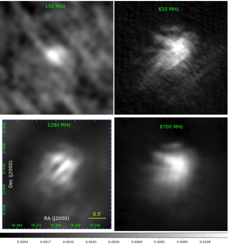
Figure 15: Radio maps of the H ii region S228 at 150, 610, 1280 and 8700 MHz, showing the distribution of ionized emission at different bands. The grey scale bar shows the intensity of radio emission in the units of mJy/beam.

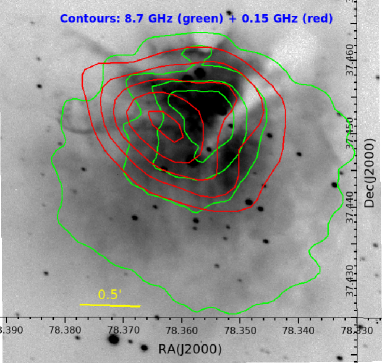
Figure 16: Comparison between emission at 8700 MHz (green contours), 150 MHz (red contours) and optical H$\alpha$ emission (grey scale background image) of the H ii region. The contours are drawn above the five times of the rms noise of the respective maps. The 8700 MHz contour levels are at 0.0005, 0.0035, 0.0065, and 0.0095 Jy/beam, whereas the 150 MHz contours are at 0.015, 0.022, 0.029, 0.036 and 0.044 Jy/beam.

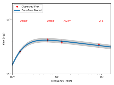
Figure 17: The SED of the H ii region S228 combining flux at 150, 610, 1280 and 8700 MHz. These measurements represent the fluxes integrated over a circular area of effective radius 0.7 arcmin ($\sim$0.7 pc). The solid line represents the fitted free-free emission model, while the shaded area represents the 1$\sigma$ uncertainty associated to the fit.

As discussed in Section 1, the cluster is associated with the H ii region S228. Figure 15 shows the maps of the H ii region at 150, 610, 1280 and 8700 MHz. These maps include GMRT observations at 610 MHz (beam size $\sim$6.6″$\times$ 3.4″, rms noise $\sim$0.2 mJy/beam) and 1280 MHz (beam size $\sim$10 ″$\times$ 8″, rms noise $\sim$0.4 mJy/beam), along with 8700 MHz map (beam size $\sim$10.5″$\times$ 7.5″, rms $\sim$0.1 mJy/beam) from the VLA archive and 150 MHz map (beam size $\sim$25″$\times$ 25″, rms $\sim$3.0 mJy/beam) from the GMRT TGSS survey.

In interferometric observations, low-level diffuse emission is often found to be missing in high-resolution and/or high-frequency observations. Despite the fact that the 150 MHz map is of low-resolution, we find that compared to other bands the ionized emission at 150 MHz, however, is seen only in the central area (e.g. see Figure 16). This could be due to the lower sensitivity of the 150 MHz observations.

Normally, the free-free emission from a homogeneous classical H ii region shows a rising SED with flux (S${}_{\nu})\propto\nu^{2}$ at lower frequencies and almost flat SED with S${}_{\nu}\propto\nu^{-0.1}$ at higher frequencies. However, the true behavior of S_ν with respect to $\nu$ strongly depends on the evolutionary status of the H ii region and can be well constrained with the thermal free-free emission modeling. Since the emission from 150 MHz is coming only from the inner region of an effective radius of $\sim$0.7′, we thus integrated fluxes at 610, 1280, and 8700 MHz maps over the same area as we did for 150 MHz. We note that before measuring the fluxes, we made low-resolution maps similar to the resolution of the 150 MHz map. Then, we convolved the maps to the exact resolution as the 150 MHz map. Figure 17 shows the radio spectrum of the H ii region along with the thermal free-free emission model (Verschuur & Kellermann, 1988) of the form:

$$S_{\nu}=\frac{2k\nu^{2}}{c^{2}}\Omega_{s}T_{e}(1-e^{-\tau_{ff}})$$ (3)

where the optical depth, $\tau_{ff}$ is expressed as

$$\tau_{ff}=0.082\times\left[\frac{EM}{{\rm cm^{-6}pc}}\right]\left[\frac{T_{e}}{{\rm K}}\right]^{-1.35}\left[\frac{\nu}{{\rm GHz}}\right]^{-2.1}.$$ (4)

In the above equations, $k$ is the Boltzmann constant, $\nu$ is the frequency, $c$ is the speed of light in vacuum, $T_{e}$ is the electron temperature, $EM$ is the emission measure, and $\Omega_{s}$ is the source solid angle. Here, we opted $\Omega_{s}$ to be $\frac{2r\pi}{6}$ for a circular aperture of radius $r$ (Mezger & Henderson, 1967). The free-free emission model resulted in the electron temperature $T_{e}\simeq 5700$ $\pm$ 400 K and emission measure $EM\simeq$3.3$\pm$0.3 $\times 10^{4}$ cm^-6 pc. We then estimated the rms electron density ($n_{e}$) using the relation, $EM$ = $n_{e}^{2}$ $\times$ $l$, where $l$ is the path length and $n_{e}$ is the electron density. This yields $n_{e}$ $\simeq$ 165 $\pm$ 10 cm^-3 using source size as the path length. We note that these values represent the average properties of the H ii region over a radius of $\sim$0.7 arcmin, and if the H ii region is clumpy, as often the case, these values can be higher at peak positions of the clumpy structures. Nonetheless, we find that our estimates are in agreement with the electron temperature in the range 0.78 $\pm$ 0.13 to 1.02 $\pm$ 0.07 K (Fernández-Martín et al., 2017) and electron density in the range 180 $\pm$ 10 to 222 $\pm$ 10 cm^-3 obtained by Fernández-Martín et al. (2017) using the nebular analysis of the optical emission lines.

For optically thin free-free emission, the radio flux density is directly proportional to the flux of the ionizing photons. And as can be seen from Figure 17, the H ii region is optically thin at high frequencies. We thus estimate the total Lyman continuum photons $N_{Lyc}$ emitted per second from the ionizing star using the total integrated flux $S_{\nu}$ of the H ii region at 8700 MHz as per the relation given in Rubin (1968)

$$N_{Lyc}=4.76\cdot 10^{48}\left(\frac{S_{\nu}}{\textnormal{Jy}}\right)\left(\frac{T_{e}}{\textnormal{K}}\right)^{-0.45}\left(\frac{\nu}{\textnormal{GHz}}\right)^{0.1}\left(\frac{d}{\textnormal{kpc}}\right)^{2}$$ (5)

where d is the distance of the region, while the meaning of the other terms are the same as in Equs. 3 & 4. Using this relation, we estimate log ($N_{Lyc}$) to be $\simeq$ 47.70.

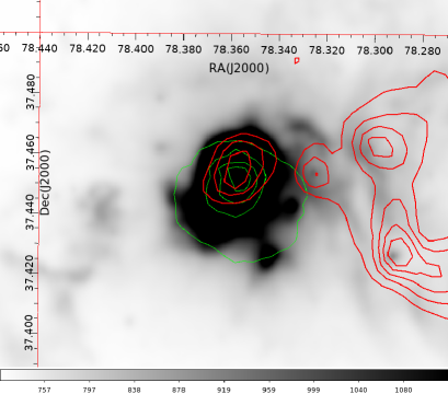
Figure 18: Image showing the distribution of WISE 12 $\mu$m (background image) emission and ionized gas emission at 8700 MHz (green contours) of S228. The red contours show the distribution of cold dust of column density greater than 3 $\times$ 10²¹ cm^-2, while the green contours reflect the 8700 MHz emission above 0.0005 Jy/beam.

In general, photo-dissociation regions (PDRs) are found at the surface layer of molecular clouds surrounding the H ii regions. PAH molecules are strong tracers of PDRs (see Samal et al., 2007, and references therein). In this regard, WISE band 3 with an effective wavelength of $\sim$12 $\mu$m is a good tracer of PDR as it contains emission lines of PAH molecules (for details, see Anderson et al., 2019). We thus consider the bright diffuse 12 $\mu$m emission around the H ii region coming from the PDR region. As can be seen from Figure 18, the 8700 MHz emission is mainly distributed within the bright PDR, implying that most of the radio emission is coming primarily from the H ii region bordered by PDR.

From spectroscopic observations, we know that the effective temperature of the massive star is $\sim$33000 $\pm$ 1000 K, thus one would expect that the minimum log($N_{lyc}$) from such a star to be $\simeq$ 48.10 photons per second (Martins et al., 2005) considering the lower limit of the temperature. We find that this value is higher than log($N_{Lyc}$) estimated from the 8700 MHz emission, implying that the fraction of the photons could have been leaked into the ISM along low-density pathways of the H ii region. We discuss this point further in Section 22.

3.2.2 Dust Distribution and Properties

To investigate the physical condition of dust around the S228 region, we derived column density and dust temperature maps by performing a pixel-to-pixel modified black-body fit to the 160, 250, 350, and 500 $\mu$m Herschel images following the procedure outlined in Battersby et al. (2011); Mallick et al. (2015). Briefly, prior to performing the modified black-body fit, we converted all the SPIRE images to the PACS flux unit (i.e., Jy pixel^-1). Then we convolved and regridded all the shorter wavelength images to the resolution and pixel size of the 500 $\mu$m map. Next, we minimize the contribution of possible excess dust emission from each image along the line-of-sight by subtracting the corresponding background flux, which we estimated from a field nearly devoid of emission. Finally, we fitted the modified black-body on these background-subtracted fluxes. For the spectral fitting, we use a dust spectral index of $\beta$=2, and the dust opacity per unit mass column density $\kappa_{\nu}=0.1~{}(\nu/1000~{}{\rm GHz})^{\beta}$ cm²gm^-1 as given in Beckwith & Sargent (1991), keeping the dust temperature T_dust, and the dust column density $N$(H${}_{2})$ as free parameters.

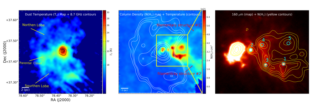
Figure 19: The left panel shows the dust temperature distribution of the S228 environment along with the distribution of ionized gas (black contours). The contour levels of the ionized gas are the same as in Figure 16. The warm dusty lobes and the heated dust of the central parental cloud are also marked. The middle panel shows the dust column density distribution along with the dust temperature contours at 17.2, 16.4, 17.6, 18.4, and 19.0 K. Two filamentary structures attached to the western clump are also marked. The right panel shows the zoomed view of the western clump. The background image is the Hershel 160 $\mu$m map and the yellow contours correspond to the dense gas above column density greater than 3 $\times$ 10²¹ cm^-2. The CUTEX identified compact sources are labelled as $\#1$ to $\#5$.

Figure 19 shows the beam-averaged low-resolution ($\sim$36${\arcsec}$) dust temperature and (left) dust column density maps (middle) of the S228 complex, along with the emission at $Herschel$ 160 $\mu$m of the high column density region. As can be seen from the figure, the temperature of the dust is between 17 and 28 K, and is distributed over a much wider area (size $\sim$10 arcmin$\times$ 20 arcmin) than the size of the cluster (i.e. radius $\sim$2.5 arcmin). The temperature map shows an almost elongated dust distribution similar to those in bipolar H ii regions (Samal et al., 2018). For example, similar to bipolar H ii regions, S228 displays two dusty lobes, each with a size of $\sim$10 arcmin  ($\sim$9.6 pc) extending nearly perpendicular to a faint warm dust lane seen at the base of the lobes. The peak of the temperature map coincides with the radio continuum emission, implying the high-temperature zone is primarily created by the intense UV radiation coming from the cluster. In contrast to the temperature map, the column density map displays a lower dust column density within the bipolar H ii region, but exhibits higher column density structures with density in the range 2$-$7 $\times$ 10²¹ cm^-2 in the western part of the H ii region. In particular, in the immediate vicinity of the H ii region lies a nearly a semicircular clumpy structure with a radius $\sim$2.8 pc and column density $>$ 3 $\times$ 10²¹ cm^-2. In general, molecular clumps have typical sizes of a few parsecs and are sites of active star formation. Thus, it could be a site of ongoing star formation as column densities above $\sim$5 $\times$ 10²¹ cm^-2 are, in general, observed to be sites of recent star formation (Lada et al., 2010). In fact, we found four 70/160 $\mu$m point sources within the condensation affirming the above hypothesis (see Figure 19 right panel). The average dust temperature of the clump is $\sim$16 K, while the average column density is $\sim$4 $\times$ 10²¹ cm^-2. The column density map also illustrates that the clump is associated with two filamentary structures in the north-western direction, and south-western directions, respectively. The north-western filament is faint and narrow with a mean temperature around 15.5 K, while the south-western filament is slightly structured with temperature in the range 14.5$-$15.5 K.

We estimated the total mass ($M_{gas}$) of the clump above column density $\sim$3 $\times$ 10²¹ cm^-2 using the following equation:

$$M=\mu{\mathrm{m}_{H}}A_{\mathrm{p}ix}\Sigma{\mathrm{H}_{2}}\,$$ (6)

where $\mu$ is the mean molecular weight, ${\mathrm{m}_{H}}$ is the mass of the hydrogen atom, $\Sigma$H₂ is the integrated H₂ column density, and $A_{\mathrm{p}ix}$ is the area of a pixel in cm^-2 at the distance of the region. The above approach yields area, mass, and density of the clump to be $\sim$28 pc², $\sim$2700 M_⊙, and $\sim$350 cm^-2, respectively. We find that the properties of the clump are similar to the nearby Ophiuchus star forming region which is one of the youngest (age $\sim$1 Myr) and closest (distance $\sim$125 pc) star-forming regions having a size of $\sim$29 pc² and mass $\sim$3100 M_☉  (Dunham et al., 2015).

The stability of a clump against gravitational collapse can be evaluated using the virial parameter (Kauffmann et al., 2013)

$$\mathit{\alpha}=1.2\left(\frac{\sigma_{\upsilon}}{\rm km\ s^{-1}}\right)^{2}\left(\frac{R_{\rm eff}}{\rm pc}\right)\left(\frac{M}{10^{3}M_{\odot}}\right)^{-1}$$ (7)

where $\sigma_{\upsilon}$ is the one-dimensional velocity dispersion, $R_{\rm eff}$ is the effective radius, and $M$ is the mass of the clump. In general, $\alpha$ $<$ 1 is suggestive of collapsing clumps while $\alpha$ $>$ 2 is suggestive of dissipating clumps and $\alpha$ $\sim$1$-$2 describes a clump that is in approximate equilibrium. However, the external pressure confined clumps with $\alpha\leq 2$ are also found to be bound and can live longer with respect to the dynamical timescale (Bertoldi & McKee, 1992). In the present case, using $\sigma$ = 1.3 km s^-1estimated over clump area from the ¹³CO map (discussed in Section 22), we find $\alpha$ $\sim$1.6, implying that clump may still be bound.

3.2.3 Herschel Compact Sources and Properties

From the right panel of Figure  19, it appears that the western clump has been fragmented into five compact structures (marked with number #1 to #5), four of which (sources #1 to #4) are protostellar as each of them is associated with a 70/160 $\mu$m point source, while the source #5 is not associated with any point like source, thus is likely a prestellar source. The presence of 70/160 $\mu$m point sources within column density peaks suggests a fresh star formation is happening at the western border of the nebula.

In order to understand the properties and evolutionary status of the 160 $\mu$m point sources, we extracted their far-infrared fluxes between 70 and 500 $\mu$m using the CUrvature Thresholding EXtractor (CUTEX) software described in Molinari et al. (2011). The CUTEX was specifically developed to optimize the source detection and extraction in the spatially varying background like the emission seen in the Herschel maps of the star-forming environments (e.g. Molinari et al., 2011). In order to estimate the envelope temperatures of the identified point sources, we fitted the observed fluxes at 70, 160, 250, and 350 $\mu$m with the modified blackbody model. Fluxes at 500 $\mu$m have been excluded, owing to the low-resolution of the 500 $\mu$m beam. This is done in order to avoid bias in the fitting procedure due to the overestimation of fluxes at 500 $\mu$m because of source confusion and the inclusion of excess background emission. We also adopted 20 percent error in flux values instead of formal photometric errors, in order to avoid any possible bias caused by underestimation of the flux uncertainties. We fitted the modified blackbody of the form, $S_{\nu}=A\,\nu^{\beta}\,B_{\nu}(T_{\rm dust})$, where $S_{\nu}$ is the observed flux distribution, $A$ is a scaling factor, $B_{\nu}(T_{\rm dust})$ is the Planck function for the dust temperature $T_{\rm dust}$ , and $\beta$ is the dust emissivity spectral index. A sample SED is shown in Figure 20 for $\beta$=2.

Having derived dust temperature, we then determined the total mass $Mass$ (gas $+$ dust) of the envelope from the dust continuum flux, $S_{\nu}$, using the following equation:

$${\rm\it Mass}=\frac{S_{\nu}\,Rd^{2}}{\kappa_{\nu}\,B_{\nu}(T_{dust})}$$ (8)

where $d$ is the distance, $R$ is the gas-to-dust ratio and is considered to be 100, and $\kappa_{\nu}$ is the dust mass opacity. We use the same dust opacity law as used in Section 3.2.2.We also estimated bolometric luminosities of the sources by integrating SED between 2 and 1000 $\mu$m. We note that, since we have not taken into account the wavelength dependence of $\beta$, therefore, the uncertainty in the mass can be of a factor of two, as discussed in Deharveng et al. (2015). Moreover, if the compact structures contain multiple point sources that are unresolved at Herschel bands, the derived mass and luminosity can be even more discrepant. Nonetheless, taking these properties of the sources at face value, we infer their likely evolutionary status by plotting them on the M${}_{env}-$ L_bol diagram. Figure 21 shows the M_env $-$ L_bol diagram of the sources along with the evolutionary tracks of protostellar objects from André et al. (2008). The figure also marks the zones of Class 0 and Class I sources. As can be seen, all the sources lie in the Class 0 zone of the plot and the evolutionary tracks in the plot indicate that these objects would evolve into stars of the mass range $\sim$3 $-$ 15 M_☉. This implies that the condensation is possibly a site of low- to intermediate-mass star formation.

4 Discussion

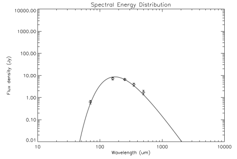
Figure 20: The SED of the embedded source #4. The circles denote the observed flux values. The black solid curve shows the grey-body fit to the data points, between 70 $\mu$m and 350 $\mu$m.

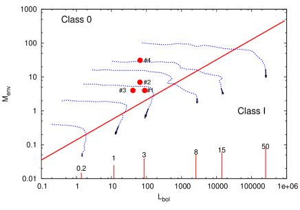
Figure 21: The (L_bol, M_env) diagram of the candidate protostars detected in the western clump (ID numbers are the same as in Figure 19). The dashed blue lines represent the evolutionary tracks from André et al. (2008). Evolution proceeds from the upper left to the lower right (indicated by arrows at the end of each track). The final stellar masses of these tracks, in solar units, are given above the vertical lines. The slanted red line corresponds to the location where 50% of the initial core mass is converted into stellar mass (Bontemps et al., 1996; André et al., 2000).

4.1 Gas Removal and Dynamical Status of the Cluster

Stellar feedback plays an important role in the removal of gas from star clusters, and subsequently cluster members dissolve completely into the galactic field (Lada & Lada, 2003). It is suggested that by comparing the age of a star in the cluster with its crossing time ($T_{cr}$) one can distinguish expanding clusters from bound clusters. According to Gieles & Portegies Zwart (2011), $\frac{T_{cr}}{Age}\sim 1$, separates bound clusters ($T_{cr}$ $<$ Age) from the unbound associations ($T_{cr}$ $>$ Age). The general definition of $T_{cr}$ (= 2$R_{H}/\sigma$) includes half mass radius ($R_{H}$) and the root-mean-square velocity dispersion ($\sigma$) of the member stars (Binney & Tremaine, 2008). Since we do not have velocity measurements of stars, we thus use the expression $T_{cr}=2.8({R_{V}^{3}}/{GM})^{1/2}$, to estimate the crossing time; where $M$ is the total mass of the system, $G$ is the gravitational constant and is $\simeq$ 0.0045 pc³ M_☉^-1 Myr^-1, and $R_{V}$ is the virial radius of the cluster (Gieles, 2010; Weidner et al., 2007). The latter is related to the $R_{H}$ as $R_{V}$ = 1.25$\times R_{H}$. We made an approximate estimate of the $R_{H}$ from the cluster center as the radius where the star count above the photometric completeness level is exactly half of the total number of stars within the cluster radius, and it turns out to be 1.07 pc. We assume that the mass of each star is roughly $\sim$0.5 M_☉, based on the fact thatf the mass distribution of stars in young clusters peaks somewhere between 0.2 to 0.7 M_☉  (Damian et al., 2021). Using this approach, we estimated $T_{cr}$ to be $\sim$3 Myr, implying that the cluster is probably marginally bound or in its initial stage of expansion, considering its age $\sim$3 Myr. It is worth noting that recently Kuhn et al. (2019) studied a sample of 28 clusters and associations with ages $\sim$1-5 Myr using PM measurements from Gaia DR2 and revealed that at least 75% of these systems are expanding.

4.2 Comparison to Other Young Clusters

Lada & Lada (2003) examined a sample of young embedded clusters within 2 kpc from the Sun with deep NIR observations and have tabulated their properties. We find that IRAS 05100+3723 is more massive than the majority of the nearby embedded clusters, except the Orion Nebula Cluster (ONC). The ONC is one of the nearest ($\sim$450 pc), young ($\sim$2 Myr), massive ($>$1000 M_☉) clusters, and hosts four massive stars of spectral type between B0 and O7 (for details see Panwar et al., 2018, and references therein). Compared to ONC, IRAS 05100+3723 is a slightly more evolved (age $\sim$3 Myr) and less massive (mass $\sim$500 M_☉) cluster and hosts only a single massive star of spectral type O8.5. We find that in terms of mass, age, and size, the studied cluster resembles the cluster Stock 8, studied by Jose et al. (2017). Stock 8 is a young cluster of age $\sim$3 Myr with the most massive star being a star of spectral type between O8 and O9 and total stellar mass $\sim$580 M_☉. We also find that IRAS 05100+3723 lies well below the mass-radius relation ($mass\propto r^{1.67}$) given by Pfalzner et al. (2016), derived for embedded clusters. This could be due to the fact that the cluster is possibly expanding and dispersing into the Galactic ISM. As a result, the cluster is not compact anymore, while embedded clusters are, in general, bound and compact systems. In fact, we find that IRAS 05100+3723 lies between embedded and loose clusters in the radius-age plane of Pfalzner & Kaczmarek (2013). Although, the total $A_{\it V}$ in the direction of the cluster is 3.3 mag, but extinction intrinsic to the cluster is only $A_{V}\sim$1 mag, which also points towards the fact that the cluster is probably no more an embedded cluster.

4.3 Star Formation Processes and Activity in the Complex

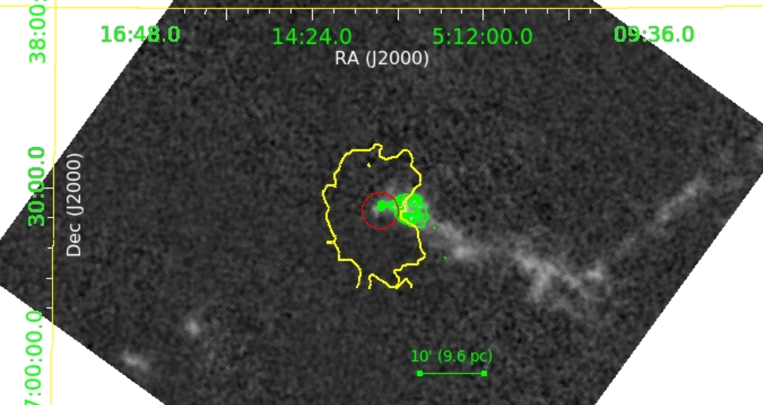
Figure 22: The image showing the distribution of ¹³CO intensity in the gray scale. The outer boundary of the $Herschel$ dust temperature map is shown with a yellow contour with $T_{d}$ = 17.2 K. The extent of the cluster is shown with a red circle. And the $Herschel$ column density contours above density 3 $\times$ 10²¹ cm^-2 (in the direction of western clump) are shown in green. The contour levels are same as given in the right panel of Figure 19.

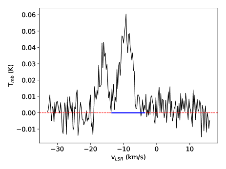
Figure 23: Average ¹³CO spectrum observed towards the S228 complex. The red and blue lines indicate the entire velocity range and velocity range associated with the S228 complex.

4.3.1 Cloud Structure, Cluster Formation, and Leaking fraction of the Ionized Gas

Figure 22 shows the ¹³CO gas distribution in the complex, along with warm and cold dust distributions derived from the temperature and column density maps. The ¹³CO intensity map was made using the observations taken with the FCRAO telescope at a spatial resolution of $\sim$45 arcsec  and a velocity resolution $\sim$0.25 km s^-1(provided by Mark Heyer, in a private communication). In the ¹³CO spectrum, two velocity components are found in the direction of S228, as shown in Figure 23. We obtained the moment maps (i.e. intensity, velocity, and velocity dispersion maps) of S228 region using its velocity component in the range $-$13.5 to $-$3.5 km s^-1, the velocity range corresponding to S228 (e.g. Chen et al., 2020). As shown in Figure 22, the distribution of the ¹³CO intensity suggests that the cluster lies at the end of a filamentary cloud. It is generally hypothesized that star-forming clouds collapse to lower-dimensional structures, producing first sheets and then filaments (Lin et al., 1965; Burkert & Hartmann, 2004; Gómez & Vázquez-Semadeni, 2014; Naranjo-Romero et al., 2020). Simulations show that such clouds experience highly non-linear gravitational acceleration as a function of position, causing the material to pile up near the cloud edge, forming a young cluster like Orion (e.g. Burkert & Hartmann, 2004; Hartmann & Burkert, 2007; Heitsch et al., 2008).

From the ¹³CO moment 1 map, we find that the V_LSR  of the ¹³CO molecular gas in the zone of the ionized gas is $\sim-$5.5 km s^-1, while the V_LSR  of the ionized gas lies in the range $-$9.4 to $-$13.6 km s^-1(Israel, 1977; Chen et al., 2020). The mean velocity of the ionized gas differs from that of the molecular gas by 4$-$8 km s^-1, implying that the ionizing gas is possibly streaming away from the cloud. This behavior is typical for H ii regions where massive stars form
near the very edge of a molecular cloud (Tenorio-Tagle, 1979) or in the center of a flat or sheet-like cloud (Bodenheimer et al., 1979), resulting in an easy flow of the ionized gas along the low-density paths of the parental cloud.

Since the morphology of the warm dust is more like the morphology of a bipolar H ii region, we thus hypothesized that the H ii region might have formed at the very end of a sheet-like or flattened cloud containing a central filament as advocated in Deharveng et al. (2015). In such clouds density along the equatorial axis is expected to be high, whereas it is expected to be low in the polar directions. Considering that the ionized gas is streaming away from the filamentary cloud at a minimum velocity of $\sim$5 km s^-1, one would expect that the ionized gas to reach $\sim$15 pc in 3 Myr (i.e the age of the cluster) from its original location. This is comparable with the projected size, $\sim$10 pc, of the warm dusty lobes seen in the temperature map. This also suggests that a fraction of the ionizing photons could have leaked into the surrounding ISM heating the dust up to several parsecs. Comparing the Lyman continuum photons expected from the ionizing star of the H ii region with the observed Lyman continuum photons derived from radio observations within the bright PDR zone, we find that approximately 60% of the Lyman photons likely have escaped from the H ii region into the diffuse ISM during the lifetime of the star. If we consider the uncertainty in the estimation of temperature and density of the ionized gas, then also the escape fraction is in the range of 40$-$50%. Our estimated escape fraction is in good agreement with the values found for other H ii regions (e.g. Oey & Kennicutt, 1997; Pellegrini et al., 2012). We note, the escape fraction also strongly depends on the age of the Lyman photon emitting source, and structure and geometry of the medium (Bodenheimer et al., 1979; Yorke et al., 1982; Howard et al., 2017); thus, may vary from region to region.

4.3.2 Compression and Confinement of Cold Gas, and Formation of Dense Clump

Figure 22 shows that the western clump (shown by green contours) lies close to the H ii region. The clump displays bow-like morphology with its apex facing the H ii region, as found in numerical simulations of H ii regions expanding into collapsing molecular clouds (e.g. Walch et al., 2015). This suggests that the over-pressured expanding H ii region possibly has compressed and pushed the western clump to its present shape. To evaluate the degree of interaction between the H ii region and the clump, we evaluated various average pressures within both the regions using the equations given below. We estimated pressure due to ionized gas of the H ii region using the following relation:

$$\begin{split}P_{\mbox{H~{}{\sc ii}~{}}}&=\sqrt{3Q_{\rm H}\over 4\pi\alpha_{rec}r^{3}}kT\\ &\approx 10^{-9}\,\left(\frac{Q_{\rm H}}{2\times 10^{49}\,\textrm{s}^{-1}}\right)^{1/2}\left(\frac{0.72\,\textrm{pc}}{r}\right)^{3/2}\,\textrm{dyn cm}^{-2}\,\end{split}$$ (9)

where $r$ is the radius, $Q_{\rm H}$ is the Lyman continuum photon responsible for the ionization of the H ii region, and $\alpha_{rec}$ is the recombination coefficient (for details see Eq. 6 of Murray, 2009). $Q_{\rm H}$ is taken to be $\sim$5.1 $\times$ 10⁴⁷ photons per second, while for the clump it is assumed to be zero as no hyper or ultra-compact H ii regions present in our high-resolution 8700 MHz image. We estimated radiation pressure using the following relation:

$$\begin{split}P_{rad}&=L/4\pi cr^{2}\\ &=4.4\times 10^{-15}\,\left(\frac{L}{\mbox{$L_{\sun}$}}\right)\left(\frac{r}{\textrm{ pc}}\right)^{-2}\,\textrm{dyn cm}^{-2}\,\end{split}$$ (10)

where we adopt the ionizing star of the H ii region as the dominant source of stellar luminosity ($L$), while in the clump the $L_{bol}$ of the most massive protostar is adopted as a proxy for stellar luminosity. We then estimated the turbulent pressure using the following relation:

$$\begin{split}P_{turb}&=\rho\sigma_{nt}^{2}\\ &=4.7\times 10^{-14}\,\left(\frac{n}{\textrm{cm}^{-3}}\right)\left(\frac{\sigma_{nt}}{\textrm{km\ s}^{-1}}\right)^{2}\,\textrm{dyn cm}^{-2}\,\end{split}$$ (11)

within the H ii region and the clump, where $\rho$ is the mass density, $n$ is the particle density, and

$$\begin{split}\sigma_{\mathrm{nt}}=\sqrt{\sigma_{\mathrm{obs}}^{2}-\sigma_{\mathrm{th}}^{2}}\end{split}$$ (12)

is the non-thermal velocity dispersion of the gas. Assuming a Gaussian distribution of the line profiles, $\sigma_{\mathrm{obs}}$ and $\sigma_{\mathrm{th}}$ can be estimated from line-widths ($\Delta V$) using

$$\sigma_{\mathrm{obs}}=\frac{\Delta V_{obs}}{2.35}\mbox{ and }\sigma_{\mathrm{th}}=\frac{\Delta V_{th}}{2.35}.$$ (13)

For the ionized gas within the H ii region, we use the observed line-width of the hydrogen radio recombination (RRL) line from Chen et al. (2020), while for the clump we use the line-width of the ¹³CO line within the clump area. For the molecular gas, we use the expression, ${\Delta V_{th}}=\sqrt{\frac{8\it{ln2}kT}{m_{\mathrm{co}}}}$, where $k$ is the Boltzmann’s constant, $T$ is the kinetic temperature of the molecular gas, and $m_{\mathrm{co}}$ is the mass of ¹³CO molecule in amu. For the ionized gas, we use the expression, ${\Delta V_{th}}=21.4\sqrt{\frac{T_{\mathrm{e}}}{10^{4}K}}$, for the hydrogen atom (Garay & Lizano, 1999), where $T_{\mathrm{e}}$ is the electron temperature. Lastly, we estimated thermal pressure using the equation:

$$\begin{split}P_{them}&=2nkT\\ &=2.8\times 10^{-16}\,\left(\frac{n_{e}}{\textrm{cm}^{-3}}\right)\left(\frac{T}{K}\right)\,\textrm{dyn cm}^{-2}\end{split}$$ (14)

where we use the mean density and mean temperature of the ionized gas and cold dust. Doing so, we estimated the total pressure within the ionized region

$$P_{ionized}=P_{\mbox{H~{}{\sc ii}~{}}}+P_{\rm{rad}}+P_{\rm{turb}}+P_{\rm{them}}$$ (15)

to be $\sim$4.5 $\times$10^-8 dyn cm^-2, while the total pressure within the clump

$$P_{\rm clump}=P_{\rm{rad}}+P_{\rm{turb}}+P_{\rm{therm}}$$ (16)

to be $\sim$2.3 $\times$10^-9 dyn cm^-2, implying that the H ii region must still be compressing the clump, as a result the clump may be under external pressure confinement. However, since the typical average pressure of the ISM is in the range of 10^-11 $-$ 10^-12 dyn cm^-2 (Bloemen, 1987; Draine, 2011); thus, we hypothesized that the H ii region must be expanding more rapidly into the ISM. In the present case, the expansion may be occurring more preferentially in the direction perpendicular to the plane of the cloud, as a result, we are observing warm dusty bipolar lobes.

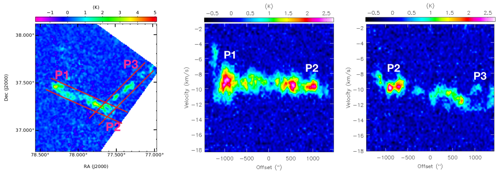
Figure 24: Position-velocity (PV) maps along the long axis of the L-shaped filament. The left panel shows the ¹³CO intensity map of the filament in Galactic longitude and latitude coordinates, the middle panel shows the PV map of the P1$-$P2 filament, while the right panel shows the PV map of the P2$-$P3 filament.

Herschel column density map shows (see Section 3.2.2) that the clump is located at the junction of two filamentary structures, while in the large-scale ¹³CO map, the clump seems to be located at the end of a long L-shaped filamentary structure. This long filamentary structure corresponds to the south-western filament seen in the Herschel image. The non-visibility of the small north-western filament in the ¹³CO map could be due to the lower sensitivity of the ¹³CO map. We note that the small-scale filamentary structures can be generated due to the self-gravity of the clump. Nonetheless, the situation is very similar to several other star-forming regions where massive clumps have been found at the merger or convergence point of filaments (e.g. Myers, 2009; Schneider et al., 2012; Kumar et al., 2020) or at the end of a large-scale filament due to edge collapse (e.g. Burkert & Hartmann, 2004; Pon et al., 2011; Yuan et al., 2020). The large-scale velocity gradients along the filaments have often been interpreted as signatures of mass flow towards star-forming clumps as a consequence of the longitudinal collapse of the filaments (Kirk et al., 2013; Ryabukhina et al., 2018; Dutta et al., 2018). Although the structure of the filament is not very smooth, which could be due to star-formation activity at multiple locations of the filament as the filament is presumably older than 3 Myr (i.e. the age of the cluster), nonetheless, we search for signatures of underlying large-scale flow (i.e. signatures of velocity gradient) along the filament’s long axis in the position-velocity (PV) map. Figure 24 shows the PV maps of the filament, extracted along its spine. To extract the PV maps, we divide the L$-$shaped filament into two parts (P1$-$P2 and P2$-$P3) as marked in Fig 24 (left panel). Figure 24 (middle panel) and Figure 24 (right panel), show the PV maps of P1$-$P2, and P2$-$P3, respectively. In PV maps, the velocity gradient in P1$-$P2 is weaker compared to the one observed for the P2$-$P3 region. Overall, the velocity gradient in the whole filament is $\sim$0.05 km s^-1. This weak velocity gradient could be due to the fact that the filament, being $\sim$3 Myr old (cluster age), star formation along the filament has already distorted its gas kinematics and also has changed the location of star-forming potential; thus, the kinematics at smaller-scale during its evolution (e.g. see discussions in Peretto et al., 2014). Nonetheless, the velocity gradient (i.e $\sim$0.1 km s^-1pc^-1) observed within P2$-$P3 is comparable to some of the large-scale filaments such as IRDC G035.39$-$00.33 ($\sim$0.2 km s^-1pc^-1; Sokolov et al., 2017) and W33 filamentary system (0.3$-$0.1 km s^-1pc^-1; Liu et al., 2021). This points to the fact that the filament has likely been dynamically active for a few Myr, thus might have supplied cold matter to the cluster location. However, high-resolution spectral observations of the filament close to the clump location will be essential to better understand the filamentary flow.

4.3.3 Second Generation Star Formation

In the filamentary environment, numerical simulations by Fukuda & Hanawa (2000) suggest that the expansion of H ii region can generate sequential waves of star-forming cores along the long axis of the filament on either side of the H ii region. This has particularly been observed in bipolar H ii regions, which are thought to be formed due to anisotropic expansion of the H ii region in a flat or sheet-like cloud containing filaments (Deharveng et al., 2015; Samal et al., 2018). Indeed, Samal et al. (2018), from the analysis of a sample of bipolar bubbles found that the most massive and compact clumps with signatures of massive star formation are always located at the waist of the bipolar bubbles and they argue that these massive clumps are the possible sites of second-generation massive- to moderate-mass star formation. Eswaraiah et al. (2019) using magnetic field geometry, strength, and comparing various pressure components, showed that the evolution and star formation of the clumps at the waists of bipolar H ii regions are indeed strongly influenced by the H ii region feedback.

The morphology of the S228 in WISE 12 $\mu$m and Herschel temperature map appears to be bipolar with two lobes extending nearly perpendicular to a faint dust lane located at the bases of the lobes. At the western waist of the bubble lies a clump whose mean temperature and mean column density are 16 K and $\sim$4 $\times$ 10²¹ cm^-2, respectively, which are conducive for the process of star formation (Lada et al., 2010; Eden et al., 2019).

Within this dense clump, as discussed in Section 3.2.3, several Class 0/I protostars and a starless core, have been identified. The fact that the age of Class 0/I sources is of the order of $\sim$10⁵ yrs (Evans et al., 2009), and these sources are located in a clump that lies at the junction point of the H ii region and filament, and the clump is under the influence of a $\sim$3 Myr old H ii region, altogether suggest that these protostars are the likley second generation stars of the complex.

5 Summary

In order to understand the formation of young massive clusters and their feedback effects on the parental cloud, we investigate the young cluster IRAS 05100+3723 and studied its environment using multiwavelength data sets.

Our findings conclude that IRAS 05100+3723 is an intermediate-mass (mass $\sim$500 M_☉) young cluster formed around 3 Myr ago at the very end of a long filamentary cloud. We find that the massive star of the cluster has created an H ii region of size $\sim$2.7 pc and temperature $\sim$5,700 K. However, it has heated the dust up to several parsecs and the distribution of the warm dust on a large-scale resembles a bipolar H ii regions. This implies that the parental cloud could be sheet-like or flattened in nature containing a central filament as suggested by Deharveng et al. (2015) for molecular clouds that host bipolar H ii regions.

Although, high-resolution kinematic studies of the filament are needed, nonetheless, from the evidences found in Sects. 4.3.1 and 4.3.2, we hypothesized that the formation of the cluster (and the H ii region) is likely due to the edge or end-dominated global collapse of the filament as advocated in Burkert & Hartmann (2004); Pon et al. (2011) and then the formation of the western clump followed. We suggest that the latter is either induced or facilitated by the compression of the expanding H ii region (Sect. 4.3.2) onto the inflowing filamentary material.

Inside the clump, we observed several far-infrared point sources of class 0/I nature. We suggest that these sources are the second-generation stars of the complex as such sources are absent in the vicinity of the ionizing star of the H ii region (see Sect. 3.2.3), they are significantly younger (age $\sim$ 10⁵ yr) than age of the H ii region (age $\sim$ 3 Myr), and they occupy a distinct location (i.e. at the interaction zone of the H ii region and filament) compared to optically visible stars. We hypothesize this scenario may be applicable to star formation at the border of several H ii region - filament environments and may be an efficient process for forming second-generation stars in molecular clouds. Future high-resolution studies of a larger sample of young H ii region - filament environments would be helpful to support our hypothesis.

We thank the anonymous referee for providing valuable comments and suggestions that improved the paper. This paper, in part, is based on observations made with MRES mounted on TNT at the Thai National Observatory (program ID C06$\_$024). TNT is operated by the National Astronomical Research Institute of Thailand (Public Organization). We acknowledge Mark Heyer for sharing FCRAO ¹³CO observations. This research has made use of the SIMBAD database, operated at CDS, Strasbourg, France. The Gaia space mission is operated by the European Space Agency (ESA). This publication uses data from the UKIDSS. This work, in part, uses the data from the Pan-STARRS1 (PS1) surveys. We acknowledge the data obtained as part of the INT Photometric H$\alpha$ Survey of the Northern Galactic Plane (IPHAS). This research uses the data obtained with the Spitzer Space Telescope. The GMRT is run by the National Centre for Radio Astrophysics of the Tata Institute of Fundamental Research. The National Radio Astronomy Observatory is a facility of the National Science Foundation operated under cooperative agreement by Associated Universities, Inc. This work has been funded by Indo-Thai project, which is supported by Ministry of Higher Education, Science, Research and Innovation (MHESI), Thailand and Department of Science and Technology (DST), India (project No. DST/INT/Thai/P-15/2019). AZ thanks the support of the Institut Universitaire de France. DKO acknowledges the support of the Department of Atomic Energy, Government of India (project No. RTI 4002). SP acknowledges the DST-INSPIRE fellowship (No. IF180092) of the Department of Science and Technology, India.

IPS (van Moorsel et al., 1996), CASA (McMullin et al., 2007), APLpy (Robitaille & Bressert, 2012), Astropy (Astropy Collaboration et al., 2013), CUTEX (Molinari et al., 2011), DS9 (Joye & Mandel, 2003; Smithsonian Astrophysical Observatory, 2000), IRAF (Tody, 1986, 1993), isochrones (Morton, 2015), STARLINK (Currie et al., 2014).

References

- Alam et al. (2015) Alam, S., Albareti, F. D., Allende Prieto, C., et al. 2015, ApJS, 219, 12, doi: 10.1088/0067-0049/219/1/12
- Anderson et al. (2019) Anderson, L. D., Makai, Z., Luisi, M., et al. 2019, ApJ, 882, 11, doi: 10.3847/1538-4357/ab1c59
- André et al. (2000) André, P., Ward-Thompson, D., & Barsony, M. 2000, in Protostars and Planets IV, ed. V. Mannings, A. P. Boss, & S. S. Russell, 59. https://arxiv.org/abs/astro-ph/9903284
- André et al. (2008) André, P., Minier, V., Gallais, P., et al. 2008, A&A, 490, L27, doi: 10.1051/0004-6361:200810957
- Ascenso et al. (2007) Ascenso, J., Alves, J., Beletsky, Y., & Lago, M. T. V. T. 2007, A&A, 466, 137, doi: 10.1051/0004-6361:20066433
- Astropy Collaboration et al. (2013) Astropy Collaboration, Robitaille, T. P., Tollerud, E. J., et al. 2013, A&A, 558, A33, doi: 10.1051/0004-6361/201322068
- Bailer-Jones (2015) Bailer-Jones, C. A. L. 2015, PASP, 127, 994, doi: 10.1086/683116
- Bailer-Jones et al. (2018) Bailer-Jones, C. A. L., Rybizki, J., Fouesneau, M., Mantelet, G., & Andrae, R. 2018, AJ, 156, 58, doi: 10.3847/1538-3881/aacb21
- Balser et al. (2011) Balser, D. S., Rood, R. T., Bania, T. M., & Anderson, L. D. 2011, ApJ, 738, 27, doi: 10.1088/0004-637X/738/1/27
- Banerjee & Kroupa (2015) Banerjee, S., & Kroupa, P. 2015, MNRAS, 447, 728, doi: 10.1093/mnras/stu2445
- Banerjee & Kroupa (2017) —. 2017, A&A, 597, A28, doi: 10.1051/0004-6361/201526928
- Barentsen et al. (2011) Barentsen, G., Vink, J. S., Drew, J. E., et al. 2011, MNRAS, 415, 103, doi: 10.1111/j.1365-2966.2011.18674.x
- Barentsen et al. (2014) Barentsen, G., Farnhill, H. J., Drew, J. E., et al. 2014, MNRAS, 444, 3230, doi: 10.1093/mnras/stu1651
- Battersby et al. (2011) Battersby, C., Bally, J., Ginsburg, A., et al. 2011, A&A, 535, A128, doi: 10.1051/0004-6361/201116559
- Beckwith & Sargent (1991) Beckwith, S. V. W., & Sargent, A. I. 1991, ApJ, 381, 250, doi: 10.1086/170646
- Bertoldi & McKee (1992) Bertoldi, F., & McKee, C. F. 1992, ApJ, 395, 140, doi: 10.1086/171638
- Bessell & Brett (1988) Bessell, M. S., & Brett, J. M. 1988, PASP, 100, 1134, doi: 10.1086/132281
- Bica et al. (2003) Bica, E., Dutra, C. M., & Barbuy, B. 2003, A&A, 397, 177, doi: 10.1051/0004-6361:20021479
- Binney & Tremaine (2008) Binney, J., & Tremaine, S. 2008, Galactic Dynamics: Second Edition (Princeton University Press)
- Bloemen (1987) Bloemen, J. B. G. M. 1987, ApJ, 322, 694, doi: 10.1086/165765
- Bodenheimer et al. (1979) Bodenheimer, P., Tenorio-Tagle, G., & Yorke, H. W. 1979, ApJ, 233, 85, doi: 10.1086/157368
- Bonnell et al. (2004) Bonnell, I. A., Vine, S. G., & Bate, M. R. 2004, MNRAS, 349, 735, doi: 10.1111/j.1365-2966.2004.07543.x
- Bontemps et al. (1996) Bontemps, S., Andre, P., Terebey, S., & Cabrit, S. 1996, A&A, 311, 858
- Borissova et al. (2003) Borissova, J., Pessev, P., Ivanov, V. D., et al. 2003, A&A, 411, 83, doi: 10.1051/0004-6361:20034009
- Burkert & Hartmann (2004) Burkert, A., & Hartmann, L. 2004, ApJ, 616, 288, doi: 10.1086/424895
- Chambers et al. (2016) Chambers, K. C., Magnier, E. A., Metcalfe, N., et al. 2016, arXiv e-prints, arXiv:1612.05560. https://arxiv.org/abs/1612.05560
- Chen et al. (2020) Chen, H.-Y., Chen, X., Wang, J.-Z., Shen, Z.-Q., & Yang, K. 2020, ApJS, 248, 3, doi: 10.3847/1538-4365/ab818e
- Chini & Wink (1984) Chini, R., & Wink, J. E. 1984, A&A, 139, L5
- Comerón & Pasquali (2005) Comerón, F., & Pasquali, A. 2005, A&A, 430, 541, doi: 10.1051/0004-6361:20041788
- Currie et al. (2014) Currie, M. J., Berry, D. S., Jenness, T., et al. 2014, in Astronomical Society of the Pacific Conference Series, Vol. 485, Astronomical Data Analysis Software and Systems XXIII, ed. N. Manset & P. Forshay, 391
- Da Rio et al. (2010) Da Rio, N., Robberto, M., Soderblom, D. R., et al. 2010, ApJ, 722, 1092, doi: 10.1088/0004-637X/722/2/1092
- Damian et al. (2021) Damian, B., Jose, J., Samal, M. R., et al. 2021, arXiv e-prints, arXiv:2101.08804. https://arxiv.org/abs/2101.08804
- Das et al. (2021) Das, S. R., Jose, J., Samal, M. R., Zhang, S., & Panwar, N. 2021, MNRAS, 500, 3123, doi: 10.1093/mnras/staa3222
- Deharveng et al. (2010) Deharveng, L., Schuller, F., Anderson, L. D., et al. 2010, A&A, 523, A6, doi: 10.1051/0004-6361/201014422
- Deharveng et al. (2015) Deharveng, L., Zavagno, A., Samal, M. R., et al. 2015, A&A, 582, A1, doi: 10.1051/0004-6361/201423835
- Dotter (2016) Dotter, A. 2016, ApJS, 222, 8, doi: 10.3847/0067-0049/222/1/8
- Draine (2011) Draine, B. T. 2011, Physics of the Interstellar and Intergalactic Medium (Princeton University Press)
- Drew et al. (2005) Drew, J. E., Greimel, R., Irwin, M. J., et al. 2005, MNRAS, 362, 753, doi: 10.1111/j.1365-2966.2005.09330.x
- Dunham et al. (2015) Dunham, M. M., Allen, L. E., Evans, Neal J., I., et al. 2015, ApJS, 220, 11, doi: 10.1088/0067-0049/220/1/11
- Dutta et al. (2015) Dutta, S., Mondal, S., Jose, J., et al. 2015, MNRAS, 454, 3597, doi: 10.1093/mnras/stv2190
- Dutta et al. (2018) Dutta, S., Mondal, S., Samal, M. R., & Jose, J. 2018, ApJ, 864, 154, doi: 10.3847/1538-4357/aadb3e
- Eden et al. (2019) Eden, D. J., Liu, T., Kim, K.-T., et al. 2019, MNRAS, 485, 2895, doi: 10.1093/mnras/stz574
- Elmegreen & Lada (1977) Elmegreen, B. G., & Lada, C. J. 1977, ApJ, 214, 725, doi: 10.1086/155302
- Eswaraiah et al. (2019) Eswaraiah, C., Lai, S.-P., Ma, Y., et al. 2019, ApJ, 875, 64, doi: 10.3847/1538-4357/ab0a0c
- Evans et al. (2009) Evans, Neal J., I., Dunham, M. M., Jørgensen, J. K., et al. 2009, ApJS, 181, 321, doi: 10.1088/0067-0049/181/2/321
- Fernández-Martín et al. (2017) Fernández-Martín, A., Pérez-Montero, E., Vílchez, J. M., & Mampaso, A. 2017, A&A, 597, A84, doi: 10.1051/0004-6361/201628423
- Feroz et al. (2009) Feroz, F., Hobson, M. P., & Bridges, M. 2009, MNRAS, 398, 1601, doi: 10.1111/j.1365-2966.2009.14548.x
- Fukuda & Hanawa (2000) Fukuda, N., & Hanawa, T. 2000, ApJ, 533, 911, doi: 10.1086/308701
- Gaia Collaboration et al. (2020) Gaia Collaboration, Brown, A. G. A., Vallenari, A., et al. 2020, arXiv e-prints, arXiv:2012.01533. https://arxiv.org/abs/2012.01533
- Gaia Collaboration et al. (2016) Gaia Collaboration, Prusti, T., de Bruijne, J. H. J., et al. 2016, A&A, 595, A1, doi: 10.1051/0004-6361/201629272
- Gaia Collaboration et al. (2018) Gaia Collaboration, Brown, A. G. A., Vallenari, A., et al. 2018, A&A, 616, A1, doi: 10.1051/0004-6361/201833051
- Garay & Lizano (1999) Garay, G., & Lizano, S. 1999, PASP, 111, 1049, doi: 10.1086/316416
- Gieles (2010) Gieles, M. 2010, in IAU Symposium, Vol. 266, Star Clusters: Basic Galactic Building Blocks Throughout Time and Space, ed. R. de Grijs & J. R. D. Lépine, 69–80, doi: 10.1017/S1743921309990895
- Gieles & Portegies Zwart (2011) Gieles, M., & Portegies Zwart, S. F. 2011, MNRAS, 410, L6, doi: 10.1111/j.1745-3933.2010.00967.x
- Gómez & Vázquez-Semadeni (2014) Gómez, G. C., & Vázquez-Semadeni, E. 2014, ApJ, 791, 124, doi: 10.1088/0004-637X/791/2/124
- Gutermuth et al. (2009) Gutermuth, R. A., Megeath, S. T., Myers, P. C., et al. 2009, ApJS, 184, 18, doi: 10.1088/0067-0049/184/1/18
- Gutermuth et al. (2005) Gutermuth, R. A., Megeath, S. T., Pipher, J. L., et al. 2005, ApJ, 632, 397, doi: 10.1086/432460
- Harayama et al. (2008) Harayama, Y., Eisenhauer, F., & Martins, F. 2008, ApJ, 675, 1319, doi: 10.1086/524650
- Hartmann & Burkert (2007) Hartmann, L., & Burkert, A. 2007, ApJ, 654, 988, doi: 10.1086/509321
- Heiter et al. (2002) Heiter, U., Kupka, F., van’t Veer-Menneret, C., et al. 2002, A&A, 392, 619, doi: 10.1051/0004-6361:20020788
- Heitsch et al. (2008) Heitsch, F., Hartmann, L. W., Slyz, A. D., Devriendt, J. E. G., & Burkert, A. 2008, ApJ, 674, 316, doi: 10.1086/523697
- Hillenbrand (1997) Hillenbrand, L. A. 1997, AJ, 113, 1733, doi: 10.1086/118389
- Howard et al. (2017) Howard, C., Pudritz, R., & Klessen, R. 2017, ApJ, 834, 40, doi: 10.3847/1538-4357/834/1/40
- Hubeny & Lanz (2011) Hubeny, I., & Lanz, T. 2011, Synspec: General Spectrum Synthesis Program. http://ascl.net/1109.022
- Hunter & Massey (1990) Hunter, D. A., & Massey, P. 1990, AJ, 99, 846, doi: 10.1086/115378
- Intema et al. (2017) Intema, H. T., Jagannathan, P., Mooley, K. P., & Frail, D. A. 2017, A&A, 598, A78, doi: 10.1051/0004-6361/201628536
- Israel (1977) Israel, F. P. 1977, A&A, 60, 233
- Jackson et al. (2006) Jackson, J. M., Rathborne, J. M., Shah, R. Y., et al. 2006, ApJS, 163, 145, doi: 10.1086/500091
- Jose et al. (2017) Jose, J., Herczeg, G. J., Samal, M. R., Fang, Q., & Panwar, N. 2017, ApJ, 836, 98, doi: 10.3847/1538-4357/836/1/98
- Joye & Mandel (2003) Joye, W. A., & Mandel, E. 2003, in Astronomical Society of the Pacific Conference Series, Vol. 295, Astronomical Data Analysis Software and Systems XII, ed. H. E. Payne, R. I. Jedrzejewski, & R. N. Hook, 489
- Kauffmann et al. (2013) Kauffmann, J., Pillai, T., & Zhang, Q. 2013, ApJ, 765, L35, doi: 10.1088/2041-8205/765/2/L35
- Kharchenko et al. (2013) Kharchenko, N. V., Piskunov, A. E., Schilbach, E., Röser, S., & Scholz, R. D. 2013, A&A, 558, A53, doi: 10.1051/0004-6361/201322302
- King (1962) King, I. 1962, AJ, 67, 471, doi: 10.1086/108756
- Kirk et al. (2013) Kirk, H., Myers, P. C., Bourke, T. L., et al. 2013, ApJ, 766, 115, doi: 10.1088/0004-637X/766/2/115
- Kroupa (2001) Kroupa, P. 2001, MNRAS, 322, 231, doi: 10.1046/j.1365-8711.2001.04022.x
- Kuhn et al. (2019) Kuhn, M. A., Hillenbrand, L. A., Sills, A., Feigelson, E. D., & Getman, K. V. 2019, ApJ, 870, 32, doi: 10.3847/1538-4357/aaef8c
- Kumar et al. (2020) Kumar, M. S. N., Palmeirim, P., Arzoumanian, D., & Inutsuka, S. I. 2020, A&A, 642, A87, doi: 10.1051/0004-6361/202038232
- Lada & Adams (1992) Lada, C. J., & Adams, F. C. 1992, ApJ, 393, 278, doi: 10.1086/171505
- Lada & Lada (2003) Lada, C. J., & Lada, E. A. 2003, ARA&A, 41, 57, doi: 10.1146/annurev.astro.41.011802.094844
- Lada et al. (2010) Lada, C. J., Lombardi, M., & Alves, J. F. 2010, ApJ, 724, 687, doi: 10.1088/0004-637X/724/1/687
- Lahulla (1985) Lahulla, J. F. 1985, A&AS, 61, 537
- Lanz & Hubeny (2003) Lanz, T., & Hubeny, I. 2003, ApJS, 146, 417, doi: 10.1086/374373
- Lawrence et al. (2007) Lawrence, A., Warren, S. J., Almaini, O., et al. 2007, MNRAS, 379, 1599, doi: 10.1111/j.1365-2966.2007.12040.x
- Lin et al. (1965) Lin, C. C., Mestel, L., & Shu, F. H. 1965, ApJ, 142, 1431, doi: 10.1086/148428
- Liu et al. (2021) Liu, X.-L., Xu, J.-L., Wang, J.-J., et al. 2021, A&A, 646, A137, doi: 10.1051/0004-6361/201935035
- Longmore et al. (2014) Longmore, S. N., Kruijssen, J. M. D., Bastian, N., et al. 2014, in Protostars and Planets VI, ed. H. Beuther, R. S. Klessen, C. P. Dullemond, & T. Henning, 291, doi: 10.2458/azu_uapress_9780816531240-ch013
- Lucas et al. (2008) Lucas, P. W., Hoare, M. G., Longmore, A., et al. 2008, MNRAS, 391, 136, doi: 10.1111/j.1365-2966.2008.13924.x
- Mallick et al. (2013) Mallick, K. K., Kumar, M. S. N., Ojha, D. K., et al. 2013, ApJ, 779, 113, doi: 10.1088/0004-637X/779/2/113
- Mallick et al. (2015) Mallick, K. K., Ojha, D. K., Tamura, M., et al. 2015, MNRAS, 447, 2307, doi: 10.1093/mnras/stu2584
- Martins et al. (2005) Martins, F., Schaerer, D., & Hillier, D. J. 2005, A&A, 436, 1049, doi: 10.1051/0004-6361:20042386
- McMullin et al. (2007) McMullin, J. P., Waters, B., Schiebel, D., Young, W., & Golap, K. 2007, in Astronomical Society of the Pacific Conference Series, Vol. 376, Astronomical Data Analysis Software and Systems XVI, ed. R. A. Shaw, F. Hill, & D. J. Bell, 127
- Mège et al. (2021) Mège, P., Russeil, D., Zavagno, A., et al. 2021, A&A, 646, A74, doi: 10.1051/0004-6361/202038956
- Mezger & Henderson (1967) Mezger, P. G., & Henderson, A. P. 1967, ApJ, 147, 471, doi: 10.1086/149030
- Minniti et al. (2010) Minniti, D., Lucas, P. W., Emerson, J. P., et al. 2010, New Astronomy, 15, 433, doi: 10.1016/j.newast.2009.12.002
- Molinari et al. (2011) Molinari, S., Schisano, E., Faustini, F., et al. 2011, A&A, 530, A133, doi: 10.1051/0004-6361/201014752
- Molinari et al. (2010) Molinari, S., Swinyard, B., Bally, J., et al. 2010, A&A, 518, L100, doi: 10.1051/0004-6361/201014659
- Morton (2015) Morton, T. D. 2015, isochrones: Stellar model grid package. http://ascl.net/1503.010
- Motte et al. (2018) Motte, F., Bontemps, S., & Louvet, F. 2018, ARA&A, 56, 41, doi: 10.1146/annurev-astro-091916-055235
- Murray (2009) Murray, N. 2009, ApJ, 691, 946, doi: 10.1088/0004-637X/691/2/946
- Myers (2009) Myers, P. C. 2009, ApJ, 700, 1609, doi: 10.1088/0004-637X/700/2/1609
- Naranjo-Romero et al. (2020) Naranjo-Romero, R., Vázquez-Semadeni, E., & Loughnane, R. M. 2020, arXiv e-prints, arXiv:2012.12819. https://arxiv.org/abs/2012.12819
- Neichel et al. (2015) Neichel, B., Samal, M. R., Plana, H., et al. 2015, A&A, 576, A110, doi: 10.1051/0004-6361/201425464
- Oey & Kennicutt (1997) Oey, M. S., & Kennicutt, R. C., J. 1997, MNRAS, 291, 827, doi: 10.1093/mnras/291.4.827
- Panwar et al. (2018) Panwar, N., Pandey, A. K., Samal, M. R., et al. 2018, AJ, 155, 44, doi: 10.3847/1538-3881/aa9f1b
- Panwar et al. (2019) Panwar, N., Samal, M. R., Pandey, A. K., Singh, H. P., & Sharma, S. 2019, AJ, 157, 112, doi: 10.3847/1538-3881/aafbe6
- Patten et al. (2006) Patten, B. M., Stauffer, J. R., Burrows, A., et al. 2006, ApJ, 651, 502, doi: 10.1086/507264
- Pecaut & Mamajek (2013) Pecaut, M. J., & Mamajek, E. E. 2013, ApJS, 208, 9, doi: 10.1088/0067-0049/208/1/9
- Pellegrini et al. (2012) Pellegrini, E. W., Oey, M. S., Winkler, P. F., et al. 2012, ApJ, 755, 40, doi: 10.1088/0004-637X/755/1/40
- Peretto et al. (2014) Peretto, N., Fuller, G. A., André, P., et al. 2014, A&A, 561, A83, doi: 10.1051/0004-6361/201322172
- Pfalzner & Kaczmarek (2013) Pfalzner, S., & Kaczmarek, T. 2013, A&A, 559, A38, doi: 10.1051/0004-6361/201322134
- Pfalzner et al. (2016) Pfalzner, S., Kirk, H., Sills, A., et al. 2016, A&A, 586, A68, doi: 10.1051/0004-6361/201527449
- Pilbratt et al. (2010) Pilbratt, G. L., Riedinger, J. R., Passvogel, T., et al. 2010, A&A, 518, L1, doi: 10.1051/0004-6361/201014759
- Pon et al. (2011) Pon, A., Johnstone, D., & Heitsch, F. 2011, ApJ, 740, 88, doi: 10.1088/0004-637X/740/2/88
- Preibisch & Mamajek (2008) Preibisch, T., & Mamajek, E. 2008, The Nearest OB Association: Scorpius-Centaurus (Sco OB2), ed. B. Reipurth, Vol. 5, 235
- Rieke & Lebofsky (1985) Rieke, G. H., & Lebofsky, M. J. 1985, ApJ, 288, 618, doi: 10.1086/162827
- Robitaille & Bressert (2012) Robitaille, T., & Bressert, E. 2012, APLpy: Astronomical Plotting Library in Python. http://ascl.net/1208.017
- Rubin (1968) Rubin, R. H. 1968, ApJ, 154, 391, doi: 10.1086/149766
- Ryabukhina et al. (2018) Ryabukhina, O. L., Zinchenko, I. I., Samal, M. R., et al. 2018, Research in Astronomy and Astrophysics, 18, 095, doi: 10.1088/1674-4527/18/8/95
- Salpeter (1955) Salpeter, E. E. 1955, ApJ, 121, 161, doi: 10.1086/145971
- Samal et al. (2018) Samal, M. R., Deharveng, L., Zavagno, A., et al. 2018, A&A, 617, A67, doi: 10.1051/0004-6361/201833015
- Samal et al. (2007) Samal, M. R., Pandey, A. K., Ojha, D. K., et al. 2007, ApJ, 671, 555, doi: 10.1086/522941
- Samal et al. (2010) —. 2010, ApJ, 714, 1015, doi: 10.1088/0004-637X/714/2/1015
- Samal et al. (2015) Samal, M. R., Ojha, D. K., Jose, J., et al. 2015, A&A, 581, A5, doi: 10.1051/0004-6361/201322787
- Schneider et al. (2012) Schneider, N., Csengeri, T., Hennemann, M., et al. 2012, A&A, 540, L11, doi: 10.1051/0004-6361/201118566
- Sharpless (1959) Sharpless, S. 1959, ApJS, 4, 257, doi: 10.1086/190049
- Sills et al. (2018) Sills, A., Rieder, S., Scora, J., McCloskey, J., & Jaffa, S. 2018, MNRAS, 477, 1903, doi: 10.1093/mnras/sty681
- Smith et al. (2010) Smith, N., Povich, M. S., Whitney, B. A., et al. 2010, MNRAS, 406, 952, doi: 10.1111/j.1365-2966.2010.16792.x
- Smithsonian Astrophysical Observatory (2000) Smithsonian Astrophysical Observatory. 2000, SAOImage DS9: A utility for displaying astronomical images in the X11 window environment. http://ascl.net/0003.002
- Sokolov et al. (2017) Sokolov, V., Wang, K., Pineda, J. E., et al. 2017, A&A, 606, A133, doi: 10.1051/0004-6361/201630350
- Swarup et al. (1991) Swarup, G., Ananthakrishnan, S., Kapahi, V. K., et al. 1991, Current Science, 60, 95
- Tenorio-Tagle (1979) Tenorio-Tagle, G. 1979, A&A, 71, 59
- Tody (1986) Tody, D. 1986, in Society of Photo-Optical Instrumentation Engineers (SPIE) Conference Series, Vol. 627, Instrumentation in astronomy VI, ed. D. L. Crawford, 733, doi: 10.1117/12.968154
- Tody (1993) Tody, D. 1993, in Astronomical Society of the Pacific Conference Series, Vol. 52, Astronomical Data Analysis Software and Systems II, ed. R. J. Hanisch, R. J. V. Brissenden, & J. Barnes, 173
- van Moorsel et al. (1996) van Moorsel, G., Kemball, A., & Greisen, E. 1996, in Astronomical Society of the Pacific Conference Series, Vol. 101, Astronomical Data Analysis Software and Systems V, ed. G. H. Jacoby & J. Barnes, 37
- Vázquez-Semadeni et al. (2019) Vázquez-Semadeni, E., Palau, A., Ballesteros-Paredes, J., Gómez, G. C., & Zamora-Avilés, M. 2019, MNRAS, 490, 3061, doi: 10.1093/mnras/stz2736
- Verschuur & Kellermann (1988) Verschuur, G. L., & Kellermann, K. I. 1988, Galactic and extra-galactic radio astronomy (Springer)
- Walborn & Fitzpatrick (1990) Walborn, N. R., & Fitzpatrick, E. L. 1990, PASP, 102, 379, doi: 10.1086/132646
- Walch et al. (2015) Walch, S., Whitworth, A. P., Bisbas, T. G., Hubber, D. A., & Wünsch, R. 2015, MNRAS, 452, 2794, doi: 10.1093/mnras/stv1427
- Weidner et al. (2010) Weidner, C., Kroupa, P., & Bonnell, I. A. D. 2010, MNRAS, 401, 275, doi: 10.1111/j.1365-2966.2009.15633.x
- Weidner et al. (2007) Weidner, C., Kroupa, P., Nürnberger, D. E. A., & Sterzik, M. F. 2007, MNRAS, 376, 1879, doi: 10.1111/j.1365-2966.2007.11580.x
- Whitney & GLIMPSE360 Team (2009) Whitney, B., & GLIMPSE360 Team. 2009, in American Astronomical Society Meeting Abstracts, Vol. 214, American Astronomical Society Meeting Abstracts #214, 210.01
- Williams & Cieza (2011) Williams, J. P., & Cieza, L. A. 2011, ARA&A, 49, 67, doi: 10.1146/annurev-astro-081710-102548
- Wright et al. (2010) Wright, E. L., Eisenhardt, P. R. M., Mainzer, A. K., et al. 2010, AJ, 140, 1868, doi: 10.1088/0004-6256/140/6/1868
- Yadav et al. (2016) Yadav, R. K., Pandey, A. K., Sharma, S., et al. 2016, MNRAS, 461, 2502, doi: 10.1093/mnras/stw1356
- Yorke et al. (1982) Yorke, H. W., Bodenheimer, P., & Tenorio-Tagle, G. 1982, A&A, 108, 25
- Yu et al. (2018) Yu, P.-C., Yu, C.-H., Lee, C.-D., et al. 2018, AJ, 155, 91, doi: 10.3847/1538-3881/aaa45b
- Yuan et al. (2020) Yuan, L., Li, G.-X., Zhu, M., et al. 2020, A&A, 637, A67, doi: 10.1051/0004-6361/201936625