A Hitting Set Relaxation for $k$-Server
and an Extension to Time-Windows

Abstract

We study the $k$-server problem with time-windows. In this problem, each request $i$ arrives at some point $v_{i}$ of an $n$-point metric space at time $b_{i}$ and comes with a deadline $e_{i}$. One of the $k$ servers must be moved to $v_{i}$ at some time in the interval $[b_{i},e_{i}]$ to satisfy this request. We give an online algorithm for this problem with a competitive ratio of $\operatorname{poly}\log(n,\Delta)$, where $\Delta$ is the aspect ratio of the metric space. Prior to our work, the best competitive ratio known for this problem was $O(k\operatorname{poly}\log(n))$ given by Azar et al. (STOC 2017).

Our algorithm is based on a new covering linear program relaxation for $k$-server on HSTs. This LP naturally corresponds to the min-cost flow formulation of $k$-server, and easily extends to the case of time-windows. We give an online algorithm for obtaining a feasible fractional solution for this LP, and a primal dual analysis framework for accounting the cost of the solution. Together, they yield a new $k$-server algorithm with poly-logarithmic competitive ratio, and extend to the time-windows case as well. Our principal technical contribution lies in thinking of the covering LP as yielding a truncated covering LP at each internal node of the tree, which allows us to keep account of server movements across subtrees. We hope that this LP relaxation and the algorithm/analysis will be a useful tool for addressing $k$-server and related problems.

1 Introduction

The $k$-Server problem, originally proposed by Manasse, McGeoch, and Sleator [MMS90], is perhaps the most well-studied problem in online algorithms. Given an $n$-point metric space and an online sequence of requests at various locations, the goal is to coordinate $k$ servers so that each request is served by moving a server to the corresponding location. The objective of the algorithm is to minimize the total distance moved by the servers (i.e., the movement cost). It has been known for more than two decades that the best deterministic competitive ratio for this problem is between $k$ [MMS90] and $2k-1$ [KP95], although determining the exact constant remains open. For randomized algorithms, even obtaining a tight asymptotic bound is still open, although there has been tremendous progress in the last decade culminating in a poly-logarithmic competitive ratio [BBMN11, BCL⁺18, BGMN19].

We focus on the $k$-server with time-windows ($k$-ServerTW) problem, where each request arrives at a location in the metric space at some time $b$ with a deadline $e\geq b$. The algorithm must satisfy the request by moving a server to that location at any point during this time interval $[b,e]$. (If $e=b$ for every request, this reduces to $k$-Server.) The techniques used to solve the standard $k$-Server problem seem to break down in the case of time-windows. Nonetheless, an $O(k\operatorname{poly}\log n)$-competitive deterministic algorithm was given for the case where the underlying metric space is a tree [AGGP17]; this gives an $O(k\operatorname{poly}\log n)$-competitive randomized algorithm for arbitrary metric spaces using metric embedding results.

For the special case of $k$-ServerTW on an unweighted star, [AGGP17] obtained competitive ratios of $O(k)$ and $O(\log k)$ using deterministic and randomized algorithms respectively. The deterministic competitive ratio of $O(k)$ extended to weighted stars as well (which is same as Weighted Paging), but a randomized (poly)-logarithmic bound already turned out to be more challenging; a bound of $\operatorname{poly}\log(n)$ was obtained only recently [GKP20]. This raises the natural question: can we obtain a poly-logarithmic competitive ratio for the $k$-ServerTW problem on general metric spaces? The technical gap between Weighted Paging and $k$-Server is substantial and bridging this gap for randomized algorithms was the preeminent challenge in online algorithms for some time. Moreover, the approaches eventually used to bridge this gap do not seem to extend to time-windows, so we have to devise a new algorithm for $k$-Server as well in solving $k$-ServerTW. We successfully answer this question.

Theorem 1.1 (Randomized Algorithm).

There is an $O(\operatorname{poly}\log(n\Delta))$-competitive randomized algorithm for $k$-ServerTW on any $n$-point metric space with aspect ratio $\Delta$.

Theorem 1.1 follows from our main technical result Theorem 1.2 below. Indeed, since any $n$-point metric space can be probabilistically approximated using $\lambda$-HSTs with height $H=O(\log_{\lambda}\Delta)$ and expected stretch $O(\lambda\log_{\lambda}n)$ [FRT04], we can set $\lambda=O(\log\Delta)$ and use the rounding algorithm from [BBMN11, BCL⁺18] to complete the reduction.

Theorem 1.2 (Fractional Algorithm for HSTs).

Fix $\delta^{\prime}\leq\nicefrac{{1}}{{n^{2}}}$. There is an $O(\operatorname{poly}(H,\lambda,\log n))$-competitive fractional algorithm for $k$-ServerTW using $\frac{k}{1-\delta^{\prime}}$ servers such that for any instance on a $\lambda$-HST with height $H$ and $\lambda\geq 10H$, and for each request interval $R=[b,e]$ at some leaf $\ell$ in this instance, there is a time in this interval at which the number of servers at $\ell$ is at least $1$.

Apart from the result itself, a key contribution of our paper is an approach to solve a new covering linear program for $k$-Server. Previous results in $k$-Server (e.g., [BCL⁺18]) used a very different LP relaxation, and it remains unclear how to extend that relaxation to the case of time-windows. The covering LP in this paper is easy to describe and flexible. It is quite natural, following from the min-cost LP formulation for $k$-Server (see §A). We hope that this relaxation, and indeed our online algorithm and accounting framework for obtaining a feasible solution will be useful for other related problems.

1.1 Our Techniques

The basis of our approach is a restatement of $k$-Server (and thence $k$-ServerTW) as a covering LP without box constraints. This LP has variables $x(v,t)$ that try to capture the event that a server leaves the subtree rooted at $v$ at some time $t$. There are several complications with this LP: apart from having an exponential number of constraints, it is too unstructured to directly tell us how to move servers. E.g., the variable for a node may increase but that for its parent or child edges may not. Or the online LP solver may increase variables for timesteps in the past, which then need to be translated to server movements at the present timestep.

Our principal technical contribution is to view this new LP as yielding “truncated” LPs, one for each internal node $v$ of the tree. This “local” LP for $v$ restricts the original LP to inequalities and variables corresponding to the subtree below $v$. This truncation is contingent on prior decisions taken by the algorithm, and so the constraints obtained may not be implied by those for the original LP. However, we show how the primal—and just as importantly—the dual solutions to local LPs can be composed to give primal/dual solutions to the original LP. These are then crucial for our accounting.

The algorithm for $k$-Server proceeds as follows. Suppose a request comes at some leaf $\ell$, and suppose $\ell$ has less than $1-\delta^{\prime}$ amounts of server at it (else we deem it satisfied):

1. Consider a vertex $v_{i}$ on the backbone (i.e., the path $\ell=v_{0},v_{1},\ldots,v_{H}=\mathbbm{r}$ from leaf $\ell$ to the root $\mathbbm{r}$). If $v_{i}$ has off-backbone children whose descendant leaves contain non-trivial amounts of server, we move servers from these descendants to $\ell$ until the total server movement has cost roughly some small quantity $\gamma$. Since the cost of server movement grows exponentially up the tree, and the movement cost is roughly the same for each $v_{i}$, more server mass is moved from closer locations. Since there are $H$ levels in the HST, the total movement cost is roughly $H\gamma$. This concludes one “round” of server movement. This server movement is now repeated over multiple rounds until $\ell$ has $1-\delta^{\prime}$ amount of server at it. (This can be thought of as a discretization of a continuous process.)

2. To account for server movement at node $v_{i}$, we raise both primal and dual variables of the local LP at $v_{i}$. The primal increase tells us which children of $v_{i}$ to move the servers from. The dual increase allows us to account for the server movement. Indeed, we ensure that the total dual increase for the local LP at each $v_{i}$—and hence by our composition operations, the dual increase for the global LP—is also approximately $\gamma$ in each round. Moreover, we show this dual scaled down by $\beta\approx O(\log n)$ is feasible. This means that the $O(H\gamma)$ cost of server movement in each round can be approximately charged to this increase of the global LP dual, giving us $H\beta=O(H\log n)$-competitiveness.

3. The choice of dual variables to raise for the local LP at node $v$ is dictated by the corresponding dual variables for the children of $v$. Each constraint in the local LP at $v$ is composed from the local constraints at some of its children. It is possible that there are several constraints at $v$ that are composed using the same constraint at a child $u$ of $v$. We maintain the invariant that the total dual values of the former is bounded by the dual value of the latter. Now, we can only raise those dual variables at $v$ where there is some slack in this invariant condition.

Finally, to extend our results to $k$-ServerTW, we say that a request $(\ell,I=[b,q])$ becomes critical (at time $q$) if the amount of server mass at $\ell$ at any time during $I$ was at most $1-\delta^{\prime}$. We proceed as above to move server mass to $\ell$. However, after servicing $\ell$, we also service active request intervals at nearby leaves: we service these piggybacked requests according to (a variation of) the earliest deadline rule while ensuring that the total cost incurred remains bounded by (a factor times) the cost incurred to service $\ell$. We use ideas from [AGGP17] (for the case of $k=1$) to find this tour, but we need a new dual-fitting-based analysis of this algorithm. Moreover, new technical insights are needed to fit this dual-fitting analysis (which works only for $k=1$) with the rest of our analytical framework. Indeed, the power of our LP relaxation for $k$-Server lies in the ease with which it extends to $k$-ServerTW.

1.2 Roadmap

In §2, we describe the covering LP relaxation for both $k$-Server and $k$-ServerTW. In §3 we define the notion of “truncated” constraints used to define local LPs at the internal nodes of the HST, and show how constraints for the children’s local LPs can be composed to get constraints for the parent LP. We then give the algorithm and analysis for the $k$-Server problem in §4 and §5 respectively: although we could have directly described the algorithm for $k$-ServerTW, it is easier to understand and build intuition for the algorithm for $k$-Server first, and then see the extension to the case of time-windows. This extension appears in §6: the algorithm is similar to that in §4, the principal addition being the issue of piggybacked requests. We give the analysis in §7: many of the ideas in §5 extend easily, but again new ideas are needed to account for the piggybacked requests. We conclude with some open problems in §8.

1.3 Related Work

The $k$-Server problem is arguably the most prominent problem in online algorithms. Early work focused on deterministic algorithms [FRR94, KP95], and on combinatorial randomized algorithms [Gro91, BG00]. $k$-Server has also been studied for special metric spaces, such as lines, (weighted) stars, trees: e.g., [CKPV91, CL91, FKL⁺91, MS91, ACN00, BBN12a, Sei01, CMP08, CL06, BBN12b, BBN10]. [BEY98] gives more background on the $k$-Server problem. Works obtaining poly-logarithmic competitive ratio are more recent, starting with [BBMN15], and more recently, by [BCL⁺18] and [Lee18]; this resulted in the first $\operatorname{poly}\log k$-competitive algorithm. ([BGMN19] gives an alternate projection-based perspective on [BCL⁺18].) A new LP relaxation was introduced by [BCL⁺18], who then use a mirror descent strategy with a multi-level entropy regularizer to obtain the online dynamics. However, it is unclear how to extend their LP when there are time-windows, even for the case of star metrics. Our competitive ratio for $k$-Server on HSTs is $\operatorname{poly}\log(n\Delta)$ as against just $\operatorname{poly}\log(k)$ in their work, but this weaker bound is in exchange for a more flexible algorithm/analysis that extends to time-windows.

Online algorithms where requests can be served within some time-window (or more generally, with delay penalties) have recently been given for matching [EKW16, AAC⁺17, ACK17], TSP [AV16], set cover [ACKT20], multi-level aggregation [BBB⁺16, BFNT17, AT19], $1$-server [AGGP17, AT19], network design [AT20], etc. The work closest to ours is that of [AGGP17] who show $O(k\log^{3}n)$-competitiveness for $k$-Server with general delay functions, and leave open the problem of getting poly-logarithmic competitiveness. Another related work is [GKP20] who show $O(\log k\log n)$-competitiveness for Weighted Paging, which is the same as $k$-Server with delays for weighted star metrics. This work also used a hitting-set LP: this was based on two different kinds of extensions of the request intervals and was very tailored to the star metric, and is unclear how to extend it even to $2$-level trees. Our new LP relaxation is more natural, being implied by the min-cost flow relaxation for $k$-Server, and extends to time-windows.

Algorithms for the online set cover problem were first given by [AAA⁺09]: this led to the general primal-dual approach for covering linear programs (and sparse set-cover instances) [BN09], and to sparse CIPs [GN14]. Our algorithm also uses a similar primal-dual approach for the local LPs defined at each node of the tree; we also need to crucially use the sparsity properties of the corresponding set-cover-like constraints.

2 A Covering LP Relaxation

For the rest of the paper, we consider the $k$-Server problem on hierarchically well-separated trees (HSTs) with $n$ leaves, rooted at node $\mathbbm{r}$ and having height $H$. (The standard extension to general metrics via tree embeddings was outlined in §1.) Define the level of a node as its combinatorial height, with the leaves at level $0$, and the root at level $H$. For a non-root node $v$, the length of the edge $(v,p(v))$ going to its parent $p(v)$ is $c_{v}:=\lambda^{\text{level}(v)}$. So leaf edges have length $1$, and edges between the root and its children have length $\lambda^{H-1}$. We assume that $\lambda\geq 10H$. For a vertex $v$, let $\chi_{v}$ be its children, $T_{v}$ be the subtree rooted at $v$, and $L_{v}$ be the leaves in this subtree. Let $n_{v}:=|T_{v}|$. For a subset $A$ of nodes of a tree $T$, let $T^{A}$ denote the minimal subtree of $T$ containing the root node and set $A$, i.e., the subtree consisting of all nodes in $A$ and their ancestors.

Request Times and Timesteps.

Let the request sequence be $\mathfrak{R}:=r_{1},r_{2},\ldots$. For $k$-Server, each request $r_{i}\in\mathfrak{R}$ is a tuple $(\ell_{q_{i}},q_{i})$ for some leaf $\ell_{q_{i}}$ and distinct request time $q_{i}\in\mathbb{Z}_{+}$, such that $q_{i-1}<q_{i}$ for all $i$. In $k$-ServerTW each request $r_{i}$ is a tuple $(\ell_{e_{i}},I_{i}=[b_{i},e_{i}])$ for a leaf $\ell_{i}$ and (request) interval $I_{i}=[b_{i},e_{i}]$ with arrival/start time $b_{i}$ and end time $e_{i}$. The algorithm sees this request $r_{i}$ at time $b_{i}$; again $b_{i-1}<b_{i}$ for all $i$. A solution must ensure that a server visit $\ell_{i}$ during interval $I_{i}$. The set of all starting and ending times of intervals are called request times; we assume these are distinct integers.

Between any two request times $q$ and $q+1$, we define a large collection of timesteps (denoted by $\tau$ or $t$)—these timesteps take on values $\{q+i\eta\}$ for some small value $\eta\in(0,1)$. (Each request arrival time is also a timestep). We use $\mathfrak{T}$ to denote the set of timesteps. Our fractional algorithm moves a small amount of server to the request location $r_{q}$ at some of the timesteps $t\in[q,q+1)$. Given a timestep $\tau$, let $\lfloor\tau\rfloor$ refer to the request time $q$ such that $\tau\in[q,q+1)$.

2.1 The Covering LP Relaxation

We first give a covering LP relaxation for $k$-Server, and then generalize it to $k$-ServerTW. Consider an instance of $k$-Server specified by an HST and a request sequence $r_{1},r_{2},\ldots$. Our LP relaxation $\mathfrak{M}$ has variables $x(v,t)$ for every non-root node $v$ and timestep $t$, where $x(v,t)$ indicates the amount of server traversing the edge from $v$ to its parent $p(v)$ at timestep $t$. The objective function is

$$\sum_{v\neq\mathbbm{r}}\sum_{t}c_{v}\;x(v,t).$$ (1)

There are exponentially many constraints. Let $A$ be a subset of leaves. Let $\boldsymbol{\tau}:=\{\tau_{u}\}_{u\in T^{A}}$ be a set of timesteps for each node in $T^{A}$, i.e., nodes in $A$ and their ancestors. These timesteps must satisfy two conditions: (i) each (leaf) $\ell\in A$ has a request at time $\lfloor\tau_{\ell}\rfloor$, and (ii) for each internal node $u\in T^{A}$, $\tau_{u}=\max_{\ell\in A\cap T_{u}}\tau_{\ell}$; i.e., $\tau_{u}$ is the latest timestep assigned to a leaf in $u$’s subtree by $\boldsymbol{\tau}$. For the tuple $(A,\boldsymbol{\tau})$, the LP relaxation contains the constraint $\varphi_{A,\boldsymbol{\tau}}$:

$$\sum_{v\in T^{A},v\neq\mathbbm{r}}x(v,(\tau_{v},\tau_{p(v)}])\geq|A|-k.$$ (2)

Define $x(v,I):=\sum_{t\in I}x(v,t)$ for any interval $I$. We now prove validity of these constraints. (In §A we show these constraints are implied by the usual min-cost flow formulation for $k$-Server, giving another proof of validity.)

Figure 1: Example of a tuple $(A,\boldsymbol{\tau})$: the set $A$ is given by the leaves in bold, the tree $T^{A}$ by the bold edges, and $\boldsymbol{\tau}$ is shown against each vertex in $T^{A}$. Bold circles on the timeline denote request arrival times, the dots denote timesteps. Each shown timestep has the corresponding request arriving at the shown leaf at the arrival time (bold dot) preceding it.

Claim 2.1.

The linear program $\mathfrak{M}$ is a valid relaxation for the $k$-Server problem.

Proof.

Consider a solution to the $k$-server instance that ensures that for a request at a leaf $\ell$ at time $q$, there is a server at $\ell$ at time $q$. We assume that this solution has the eagerness property—if leaves $\ell$ and $\ell^{\prime}$, requested at times $q$ and $q^{\prime}$ respectively, are two consecutive locations visited by a server, the server moves from $q$ to $q^{\prime}$ at timestep $q+\eta$ (which is less than $q^{\prime}$).

Now for a constraint of the form (2), let $A_{1},A_{2},\ldots,A_{k}$ be the subsets of $A$ that are served by the different servers (some of these sets may be empty). Define $x_{i}(v,t)\leftarrow 1$ if server $i$ crosses the edge $(v,p(v))$ from $v$ to $p(v)$ (i.e., upwards) at timestep $t$, and $0$ otherwise. We show that

$$\sum_{v\in T(A_{i}),v\neq\mathbbm{r}}x_{i}(v,(\tau_{v},\tau_{p(v)}])\geq|A_{i}|-1.$$

Defining $x(v,t):=\sum_{i}x_{i}(v,t)$ by summing over all $i$ gives (2). For any server $i$ and set $A_{i}$, define $E^{\prime}$ to be the edges $(v,p(v))$ for which $x_{i}(v,(\tau_{v},\tau_{p(v)}])=1$. If $|E^{\prime}|<|A_{i}|-1$, then deleting the edges in $E^{\prime}$ from the tree leaves a connected component $C$ with at least two vertices from $A_{i}$. Server $i$ serves at least two leaf vertices $C\cap A_{i}$, say $v,w$, requested at times $q_{v}=\lfloor\tau_{v}\rfloor,q_{w}=\lfloor\tau_{w}\rfloor$ respectively. Say $q_{v}<q_{w}$, and let $u$ be the least common ancestor of $v,w$. Notice that $\tau_{u}\geq\tau_{v}$, and if the path from $v$ to $u$ is labeled $v_{0}=v,v_{1},\ldots,v_{h}=u$, then the intervals $(\tau_{v_{i}},\tau_{v_{i+1}}]$ partition $(\tau_{v},\tau_{u}]$. Since the server is at $v$ at timestep $\tau_{v}$ (by the construction above) and is at $w$ at time $q_{w}\leq\tau_{w}$, there must be an edge $(v_{i},v_{i+1})$ such that it crosses this edge upwards during $(\tau_{v_{i}},\tau_{v_{i+1}}]$. Then this edge should be in $E^{\prime}$, a contradiction. ∎

Remark 2.2.

We could have replaced the constraint (2) by its simpler version involving $x_{i}(v,(q_{v},q_{p(v)}])$, where $q_{v}:=\lfloor\tau_{v}\rfloor$: that would be valid and sufficient. However, since our algorithm works at the level of timesteps, it is convenient to use (2).

Extension to Time-Windows.

We now extend these ideas to $k$-ServerTW. In constraint (2) for a pair $(A,\boldsymbol{\tau})$, the timesteps for ancestors of (a leaf in) $A$ could be inferred from the values assigned by $\tau$ to $A$. We now generalize this by (i) allowing $A$ to contain non-leaf nodes, as long as they are independent (in terms of the ancestor-descendant relationship), and (ii) the timestep assigned to an internal node is at least that of each of its descendants in $A$. Formally, consider a tuple $(A,f,\boldsymbol{\tau})$, where $A$ is a subset of tree nodes such that no two of them have an ancestor-descendant relationship, the function $f:A\to\mathfrak{R}$ maps each node $v\in A$ to a request $(\ell_{v},[b_{v},e_{v}])$ given by a leaf $\ell_{v}\in T_{v}$ and an interval $[b_{v},e_{v}]$ at $\ell_{v}$, and the assignment $\boldsymbol{\tau}$ maps each node $u\in T^{A}$ to a timestep $\tau_{u}$ satisfying the following two (monotonicity) properties:

• For each node $v\in T^{A}$, $\tau_{v}\geq\max_{u\in A\cap T_{v}}e_{u}.$

• If $v_{1},v_{2}$ are two nodes in $T^{A}$ with $v_{1}$ being the ancestor of $v_{2}$, then $\tau_{v_{1}}\geq\tau_{v_{2}}.$

Given such a tuple $(A,f,\boldsymbol{\tau})$, we define the constraint $\varphi_{A,f,\boldsymbol{\tau}}$

$$\sum_{v\in A,v\neq\mathbbm{r}}x(v,(b_{v},\tau_{p(v)}])+\sum_{v\in T^{A}\setminus A,v\neq\mathbbm{r}}x(v,(\tau_{v},\tau_{p(v)}])\geq|A|-k.$$ (3)

Note the differences with constraint (2): the LHS for a node $v\in A$ has a longer interval starting from $b_{v}$ instead of from $\tau_{v}$. Also, (3) does not use the timesteps $\{\tau_{v}\}_{v\in A}$: these will be useful later in defining the truncated constraints. In the special case of $k$-Server where $e_{v}=b_{v}+1$, the above constraint is similar to (2), though the terms for nodes in $A$ differ slightly. The objective function is the same as (1). We denote this LP by $\mathfrak{M}_{TW}$.

Figure 2: Example of a tuple $(A,f,\boldsymbol{\tau})$ for $k$-ServerTW: the set $A$ is given by the bold nodes, the tree $T^{A}$ by the bold edges, and $\boldsymbol{\tau}$ is shown against each internal vertex in $T^{A}$. Arrows indicate the mapping $f$ to a leaf request interval.

Claim 2.3.

The linear program $\mathfrak{M}_{TW}$ is a valid relaxation for $k$-ServerTW.

Proof.

Consider a solution to the instance that ensures a server moves only when a request becomes critical (although at this time, it can serve several outstanding requests). Now for a constraint of the form (3), let $L$ denote the set of leaves corresponding to the nodes in $A$. let $L_{1},L_{2},\ldots,L_{k}$ be the subsets of $L$ that are served by the different servers (some of these sets may be empty), and let $A_{i}$ be the subset of $A$ corresponding to $L_{i}$. Define $x_{i}(v,t)\leftarrow 1$ if server $i$ crosses the edge $(v,p(v))$ at time $t$, and $x(v,t):=\sum_{i}x_{i}(v,t)$. We show that

$$\sum_{v\in A,v\neq\mathbbm{r}}x_{i}(v,(b_{v},\tau_{p(v)}])+\sum_{v\in T^{A}\setminus A,v\neq\mathbbm{r}}x_{i}(v,(\tau_{v},\tau_{p(v)}])\geq|A_{i}|-1;$$

recall that $b_{v},v\in A,$ is the starting time of the request interval given by $f(v)$. Summing the above inequality over all $i$ gives (3).

For sake of brevity, let $I_{v}$ denote the interval $(b_{v},\tau_{p(v)}]$ or $(\tau_{v},\tau_{p(v)}]$ depending on whether $v\in A$. Define $E^{\prime}$ as the set of edges $(v,p(v))$ for which $x_{i}(v,I_{v})\geq 1$. We need to show that $|E|\geq|A_{i}|-1$. Suppose not. Then deleting the edges in $E^{\prime}$ from the tree $T$ leaves a connected component with at least two vertices from $A_{i}$.

Call this component $C$, and let $u,v$ be two distinct vertices in $A_{i}\cap C$. Let $f(u)$ and $f(v)$ be $(\ell_{u},R_{u}=(b_{u},e_{u}]),(\ell_{v},R_{v}=(b_{v},e_{v}])$ respectively. Let $w$ be the lca of $\ell_{u}$ and $\ell_{v}$. Note that $w$ is also the lca of $u$ and $v$. Suppose server $i$ satisfies $R_{u}$ before satisfying $R_{v}$. We claim that the server $i$ reaches $w$ at some time during $(b_{u},\tau_{w}]$. To see this, we consider two cases:

• Server $i$ visits $u$ at time $e_{u}$ when the request $R_{u}$ becomes critical: Since it reaches $v$ by time $e_{v}$, it must have visited $w$ during $(e_{u},e_{v}]\subseteq(b_{u},\tau_{w}]$.

• Server $i$ visits $u$ before $R_{u}$ becomes critical. In this case, it would have visited $u$ strictly after $b_{u}$ ((because all start and end times of requests are distinct). Since it reaches $w$ at or before $e_{v}\leq\tau_{w}$, the desired statement holds in this case as well.

Let the sequence of nodes in $B$ from $u$ to $w$ be $v_{0}=u,v_{1},\ldots,v_{h}=w.$ Note that all the edges $(v_{i},p(v_{i})),i<h,$ lie below $w$ and so are not in $E^{\prime}$. Observe that the intervals $I_{v_{i}},i=0,\ldots,h-1$, partition $(b_{u},\tau_{w}]$. As outlined in the two cases above, the server $i$ leaves $u$ strictly after $b_{u}$ and reaches $w$ by time $\tau_{w}$. Therefore, there must be an edge $(v_{i},p(v_{i})),i<h$, such that it crosses this edge during $I_{v_{i}}$. Then this edge should be in $E^{\prime}$, a contradiction. ∎

3 The Local LPs: Truncation and Composition

We maintain a collection of local LPs $\mathfrak{L}^{v}$, one for each internal vertex $v$ of the tree. While the constraints of local LPs for the non-root nodes are not necessarily valid for the original $k$-Server instance, those in the local LP $\mathfrak{L}^{\mathbbm{r}}$ are implied by constraints of $\mathfrak{M}$ or $\mathfrak{M}_{TW}$. This gives us a handle on the optimal cost. The constraints in the local LP at a node are related to those in its children’s local LPs, allowing us to relate their primal/dual solutions, and their costs.

To define the local LPs, we need some notation. Our (fractional) algorithm ${\mathcal{A}}$ moves server mass around over timesteps. In the local LPs, we define constraints based on the state of our algorithm ${\mathcal{A}}$. Let $k_{v,t}$ be the server mass that ${\mathcal{A}}$ has in $v$’s subtree $T_{v}$ at timestep $t$ (when $v$ is a leaf, this is the amount of server mass at $v$ at timestep $t$). We choose three non-negative parameters $\delta,\delta^{\prime},\gamma$. The first two help define lower and upper bounds on the amount of (fractional) servers at any leaf, and $\gamma$ denotes the granularity at which movement of server mass happens. We ensure $\delta^{\prime}\gg\delta\gg\gamma$, and set $\delta^{\prime}=\frac{1}{n^{2}},\delta=\frac{1}{10n^{3}},\gamma=\frac{1}{n^{4}}$.

Definition 3.1 (Active and Saturated Leaves).

Given an algorithm ${\mathcal{A}}$, a leaf $\ell$ is active if it has at least $\delta$ amount of server (and inactive otherwise). The leaf is saturated if $\ell$ has more than $1-\delta^{\prime}$ amount of server (and unsaturated otherwise).

The server mass at each location should ideally lie in the interval $[\delta,1-\delta^{\prime}]$, but since we move servers in discrete steps, we maintain the following (slightly weaker) invariant:

Invariant (I1).

The server mass at each leaf lies in the interval $[\nicefrac{{\delta}}{{2}},1-\nicefrac{{\delta^{\prime}}}{{2}}].$

Constraints of $\mathfrak{L}^{v}$ are defined using truncations of the constraints $\varphi_{A,\boldsymbol{\tau}}$. For a node $v$ and subset of nodes $A$ in $T$, let the subtree $T_{v}^{A}$ be the minimal subtree of $T_{v}$ containing $v$ and all the nodes in $A\cap T_{v}$.

Definition 3.2 (Truncated Constraints).

Consider a node $v$, a subset $A$ of leaves in $T$ and a set $\boldsymbol{\tau}:=\{\tau_{u}\}_{u\in T^{A}_{v}}$ of timesteps satisfying the conditions: (i) each (leaf) $\ell\in A$ has a request at time $\lfloor\tau_{\ell}\rfloor$, and (ii) for each internal node $u\in T^{A}_{v},\tau_{u}=\max_{\ell\in A}\cap T_{v}$. The truncated constraint $\varphi_{A,\boldsymbol{\tau},v}$ is defined as:

$$\sum_{u:u\neq v,u\in T^{A}_{v}}y^{v}(u,(\tau_{u},\tau_{p(u)}])\geq|A\cap T_{v}|-k_{v,\tau_{v}}-2\delta(n-n_{v});$$ (4)

recall that $k_{v,\tau_{v}}$ is the amount of server mass in $T_{v}$ at the end of timestep $\tau_{v}$. We say that the truncated constraint $\varphi_{A,\boldsymbol{\tau},v}$ ends at $\tau_{v}$.

The truncated constraint $\varphi_{A,\boldsymbol{\tau},v}$ can be thought of as truncating an actual LP constraint of the form (2) for the nodes in $T_{v}^{A}$ only. One subtle difference is the last term that weakens the constraint slightly; we will see in Lemma 3.5 that this weakening is crucial. The truncated constraint $\varphi_{A,f,\boldsymbol{\tau},v}$ in case of $k$-ServerTW is defined analogously: given a node $v$, a tuple $(A,f,\boldsymbol{\tau})$ satisfying the conditions stated above (3) with the restriction that $A$ lies in $T_{v}$ and $\boldsymbol{\tau}$ is defined for nodes in $T_{v}^{A}$ only, the truncated constraint $\varphi_{A,f,\boldsymbol{\tau},v}$ (ending at $\tau_{v}$) is defined as (see 6.1 for a formal definition):

$$\sum_{u\in A\cap T_{v},u\neq v}y^{v}(u,(b_{u},\tau_{p(u)}])+\sum_{u\in T^{A}_{v}\setminus A,u\neq v}y^{v}(u,(\tau_{u},\tau_{p(u)}])\geq|A\cap T_{v}|-k_{v,\tau_{v}}-2\delta(n-n_{v})$$ (5)

A few remarks about the truncation: first, this truncated constraint uses local variables $y^{v}$ that are “private” for the node $v$ instead of the global variables $x$. In fact, we can think of $x$ as denoting variables $y^{\mathbbm{r}}$ local to the root, and therefore $\varphi_{A,\boldsymbol{\tau},\mathbbm{r}}=\varphi_{A,\boldsymbol{\tau}}$ (or $\varphi_{A,f,\boldsymbol{\tau},\mathbbm{r}}=\varphi_{A,f,\boldsymbol{\tau}}$). Second, a truncated constraint is not necessarily implied by the LP relaxation $\mathfrak{M}$ (or $\mathfrak{M}_{TW}$) even when we replace $y^{v}$ by $x$, since a generic algorithm is not constrained to maintain $k_{v,\tau_{v}}$ servers in subtree $T_{v}$ after timestep $\tau_{v}$. But, at the root (i.e., when $v=\mathbbm{r}$), we always have $k_{v,\tau_{v}}=k$ and the last term is $0$, so replacing $y^{\mathbbm{r}}$ by $x$ in its constraints gives us constraints of the form (2) from the actual LP.

Definition 3.3 ($\bot$-constraints).

A truncated constraint where $|A|=1$ is called a $\bot$-constraint.

Such $\bot$-constraints play a special role when a subtree has only one active leaf, namely the requested leaf. In the case of $k$-Server, if $|A|=1$ then the constraint (4) has no terms on the LHS but a positive RHS, so it can never be satisfied. Nevertheless, such constraints will be useful when forming new constraints by composition.

Composing Truncated Constraints.

The next concept is that of constraint composition: a truncated constraint $\varphi_{A,\boldsymbol{\tau},v}$ can be obtained from the corresponding truncated constraints for the children of $v$. Consider a subset $X$ of $v$’s children. For $u\in X$, let $C_{u}:=\varphi_{A(u),\boldsymbol{\tau}(u),u}$ be a constraint in ${\mathfrak{L}}^{u}$ ending at $\tau_{u}:=\tau(u)_{u}$, given by some linear inequality $\langle a^{C_{u}},y^{u}\rangle\geq b^{C_{u}}$. Then defining $A:=\cup_{u\in X}A(u)$ and $\tau:T^{A}\to\mathfrak{T}$ obtained by extending maps $\boldsymbol{\tau}(u)$ and setting $\tau_{v}=\max_{u\in X}\tau_{u}$, the constraint $\varphi_{A,\boldsymbol{\tau},v}$ is written as:

$$\sum_{u\in X}\bigg{(}y^{v}(u,(\tau_{u},\tau_{v}])+\langle a^{C_{u}},y^{v}\rangle\bigg{)}\geq\sum_{u\in X}b^{C_{u}}-\Big{(}k_{v,\tau_{v}}-\sum_{u\in X}k_{u,\tau_{u}}\Big{)}+2\delta\Big{(}n_{v}-\sum_{u\in X}n_{u}\Big{)}.$$ (6)

The constraints $\varphi_{A(u),\boldsymbol{\tau}(u),u}$ used their local variables $y^{u}$, whereas this new constraint uses $y^{v}$. Every constraint in ${\mathfrak{L}}^{v}$ can be obtained this way, and so the constraints of $\mathfrak{L}^{\mathbbm{r}}$ (which are implied by $\mathfrak{M}$) can be obtained by recursively composing truncated constraints for its children’s local LPs. In case of $k$-ServerTW, the composition operation holds for the constraints $\varphi_{A,f,\boldsymbol{\tau},v}$: a minor change is that the terms in LHS involving a vertex $u\in A$ have $y^{v}(u,(b_{u},\tau_{v}])$, where $b_{u}$ is the starting time of the request corresponding to $f(u)$. (We see the details later in (22).)

3.1 Constraints in Terms of Local Changes

The local constraints (4) and the composition rule (6) are written in terms of $k_{u,\tau_{u}}$, the amount of server that our algorithm ${\mathcal{A}}$ places at various locations and times. It will be more convenient to rewrite them in terms of server movements in ${\mathcal{A}}$.

Definition 3.4 ($g,r,D$).

For a vertex $v$ and timestep $t$, let the give $g(v,t)$ and the receive $r(v,t)$ denote the total (fractional) server movement out of and into the subtree $T_{v}$ on the edge $(v,p(v))$ at timestep $t$. For interval $I$, let $g(v,I):=\sum_{t\in I}g(v,t)$ and define $r(v,I)$ similarly, and define the “difference” $D(v,I):=g(v,I)-r(v,I)$.

Restating the composition rule in terms of the quantities $D$ defined above shows the utility of the extra term on the RHS of the truncated constraint.

Lemma 3.5.

Consider a vertex $v$, a timestep $\tau$ and a subset $X$ of children of $v$ such that at timestep $\tau$ all active leaves in $T_{v}$ are descendants of the nodes in $X$. For each $u\in X$, consider a truncated constraint $C_{u}:=\varphi_{A(u),\boldsymbol{\tau}(u),u}$ given by some linear inequality $\langle a^{C_{u}},y^{u}\rangle\geq b^{C_{u}}$. Define $(A,\boldsymbol{\tau})$ as in (6) with $\tau:=\tau_{v}$, and assume Invariant (I1) holds. Then the truncated constraint $\varphi_{A,\boldsymbol{\tau},v}$ from (6) implies the inequality :

$$\sum_{u\in X}\bigg{(}y^{v}(u,(\tau_{u},\tau_{v}])+\langle a^{C_{u}},y^{v}\rangle\bigg{)}\geq\sum_{u\in X}\bigg{(}D(u,(\tau_{u},\tau_{v}])+b^{C_{u}}\bigg{)}+\big{(}n_{v}-\sum_{u\in X}n_{u}\big{)}\delta,$$ (7)

We call this the composition rule. An analogous statement holds for a tuple $(A,f,\boldsymbol{\tau})$ for a vertex $v$ in the case of $k$-ServerTW, except that $\tau_{u}$ is replaced by $b_{u}$ for every vertex $u\in A$ on the LHS (see (22)).

Proof.

Note that $k_{v,\tau_{v}}=\sum_{u\in X}k_{u,\tau_{v}}+\sum_{w\not\in X}k_{w,\tau_{v}}=\sum_{u\in X}k_{u,\tau_{u}}-\sum_{u\in X}D(u,(\tau_{u},\tau_{v}])+\sum_{w\not\in X}k_{w,\tau_{v}}.$ in (6) gives

$$\sum_{u\in X}\bigg{(}y^{v}(u,(\tau_{u},\tau_{v}])+\langle a^{C_{u}},y^{v}\rangle\bigg{)}\geq\sum_{u\in X}\Big{(}D(u,(\tau_{u},\tau_{v}])+b^{C_{u}}\Big{)}-\sum_{w\not\in X}k_{w,\tau_{v}}+2\delta\Big{(}n_{v}-\sum_{u\in X}n_{u}\Big{)}.$$

Finally, since all active leaves in $T_{v}$ at timestep $\tau_{v}$ are descendants of $X$, Invariant (I1) implies that $\sum_{w\not\in X}k_{w,\tau_{v}}\leq\delta\sum_{w\notin X}n_{w}\leq\delta\left(n_{v}-\sum_{u\in X}n_{u}\right)$. This is where the weakening in (4) is useful. ∎

3.2 Timesteps and Constraint Sets

Recall that $\mathfrak{T}$ is the set of all timesteps. For each vertex $v$ we define a subset $\mathcal{R}(v)\subseteq\mathfrak{T}$ of relevant timesteps, such that the local LP $\mathfrak{L}^{v}$ contains a non-empty set of constraints ${\mathfrak{L}}^{v}(\tau)$ for each $\tau\in\mathcal{R}(v)$. Should we say what the variables are in this LP? Each constraint in ${\mathfrak{L}}^{v}(\tau)$ is of the form $\varphi_{A,\boldsymbol{\tau},v}$ for a tuple $(A,\boldsymbol{\tau})$ ending at $\tau$. Overloading notation, let ${\mathfrak{L}}^{v}:=\bigcup_{\tau\in\mathcal{R}(v)}{\mathfrak{L}}^{v}(\tau)$ denote the set of all constraints in the local LP at $v$. The objective function of this local LP is $\sum_{u\in T_{v},\tau}c_{u}\;y^{v}(u,\tau)$. What does $\tau$ sum over?

The timesteps in $\mathcal{R}(v)$ are partitioned into $\mathcal{R}^{s}(v)$ and $\mathcal{R}^{ns}(v)$, the solitary and non-solitary timesteps for $v$. The decision whether a timestep belongs to $\mathcal{R}(v)$ is made by our algorithm. and is encoded by adding $\tau$ to either $\mathcal{R}^{s}(v)$ or $\mathcal{R}^{ns}(v)$. For each timestep $\tau\in\mathcal{R}^{s}(v)$, the algorithm creates a constraint set ${\mathfrak{L}}^{v}(\tau)$ consisting of a single $\bot$-constraint (recall 3.3); for each timestep $\tau\in\mathcal{R}^{ns}(v)$ it creates a constraint set ${\mathfrak{L}}^{v}(\tau)$ containing only non-$\bot$-constraints obtained by composing constraints from ${\mathfrak{L}}^{w}(\tau_{w})$ for some children $w$ of $v$ and timesteps $\tau_{w}\in\mathcal{R}(w)$, where $\tau_{w}\leq\tau$.

For each $\tau$, a constraint $C\in{\mathfrak{L}}^{v}(\tau)$ corresponds to a dual variable $z_{C}$, which is raised only at timestep $\tau$. We ensure the following invariant.

Invariant (I2).

At the end of each timestep $\tau\in\mathcal{R}^{ns}(v)$, the objective function value of the dual variables corresponding to constraints in ${\mathfrak{L}}^{v}(\tau)$ equals $\gamma$. I.e., if a generic constraint $C$ is given by $\langle a^{C}\cdot y^{v}\rangle\geq b^{C}$, then

$$\sum_{C\in{\mathfrak{L}}^{v}(\tau)}b^{C}\cdot z_{C}=\gamma\qquad\forall\tau\in\mathcal{R}^{ns}(v).$$ (I2)

Furthermore, $b^{C}>0$ for all $C\in\mathfrak{L}^{v}(\tau)$ and $\tau\in\mathcal{R}(v)$.

No dual variables $z_{C}$ are defined for $\bot$-constraints, and (the first statement of) Invariant (I2) does not apply to timesteps $\tau\in\mathcal{R}^{s}(v)$. In the following sections, we show how to maintain a dual solution that is feasible for $\mathfrak{D}^{v}$ (the dual LP for $\mathfrak{L}^{v}$) when scaled down by some factor $\beta=\operatorname{poly}\log(n\lambda)$.

Awake Timesteps.

For a vertex $v$, we maintain a subset ${\sf Awake}(v)$ of awake timesteps. The set ${\sf Awake}(v)$ has the property that it contains all the solitary timesteps, i.e., $\mathcal{R}^{s}(v)$, and some non-solitary ones. Hence $\mathcal{R}^{s}(v)\subseteq{\sf Awake}(v)\subseteq\mathcal{R}^{s}\cup\mathcal{R}^{ns}(v)=\mathcal{R}(v)$. Whenever we add a timestep to $\mathcal{R}(v)$, we initially add it to ${\sf Awake}(v)$; some of the non-solitary ones subsequently get removed. A timestep $\tau$ is awake for vertex $v$ at some moment in the algorithm if it belongs to ${\sf Awake}(v)$ at that moment. For any vertex $v$, define

$${\sf prev}(v,\tau):=\arg\max\{\tau^{\prime}\in{\sf Awake}(v)\mid\tau^{\prime}\leq\tau\}$$ (8)

Note that as the set ${\sf Awake}(v)$ evolves over time, so does the identity of ${\sf prev}(v,\tau)$. We show in Claim 5.5 that ${\sf prev}$ is well-defined for all relevant $(v,\tau)$ pairs. Motivate this better?

Starting configuration.

At the beginning of the algorithm, assume that the root has $2k$ “dummy” leaves as children, each of which has server mass $\nicefrac{{1}}{{2}}$ at time $q=0$. All other leaves of the tree have mass $\delta/2$. (This ensures Invariant (I1) holds.) No requests arrive at any dummy leaf $v$; moreover, we add a $\bot$-constraint $\varphi_{A,\boldsymbol{\tau},v}$, where $A=\{v\}$ and $\tau_{v}=0$. Should we say why? Assuming this starting configuration only changes the cost of our solution by at most an additive term of $O(k\Delta)$, where $\Delta$ is the aspect ratio of the metric space.

4 Algorithm for $k$-Server

We now describe our algorithm for $k$-Server. At request time $q$, the request arrives at a leaf $\ell_{q}$. The main procedure calls local update procedures for each ancestor of $\ell_{q}$. Each such local update possibly moves servers to $\ell_{q}$, and also adds constraints to the local LPs and raises the primal/dual values to account for this movement. We use $\textsf{ReqLoc}(\tau)$ to denote the location of request with deadline at time $\lfloor\tau\rfloor$, i.e., $\ell_{\lfloor\tau\rfloor}$.

4.1 The Main Procedure

In the main procedure of Algorithm 1, let the backbone be the leaf-root path $\ell_{q}=v_{0},v_{1},\ldots,v_{H}=\mathbbm{r}$. We move servers to $\ell_{q}$ from other leaves until it is saturated: this server movement happens in small discrete increments over several timesteps. Each iteration of the while loop in line (1) corresponds to a distinct timestep $\tau$. Let ${\sf activesib}(v,\tau)$ be the siblings $v^{\prime}$ of $v$ with active leaves in their subtrees $T_{v^{\prime}}$ (at timestep $\tau$). Let $i_{0}$ be the smallest index with non-empty ${\sf activesib}(v_{i_{0}},\tau)$. The procedure SimpleUpdate adds a $\bot$-constraint to each of the sets $\mathfrak{L}^{v_{i}}(\tau)$ for $i=0,\ldots,i_{0}$. For $i>i_{0}$, the procedure FullUpdate adds (non-$\bot$) constraints to $\mathfrak{L}^{v_{i}}(\tau)$. If ${\sf activesib}(v_{i},\tau)$ is non-empty, it also transfers some servers from the subtrees below ${\sf activesib}(v_{i},\tau)$ to $\ell_{q}$.

0.1 foreach $q=1,2,\ldots$ do

0.2       get request $r_{q}$; let the path from $r_{q}$ to the root be $\ell_{q}=v_{0},v_{1},\ldots,v_{H}=\mathbbm{r}$.;

0.3       $\tau\leftarrow q+\eta$, the first timestep after $q$. ;

0.4       while $k_{v_{0},\tau}\leq 1-\delta^{\prime}$  do

0.5             let $i_{0}\leftarrow$ smallest index such that ${\sf activesib}(v_{i_{0}},\tau)\neq\varnothing$.

0.6             for $i=0,\ldots,i_{0}$ do call $\textsc{SimpleUpdate}(v_{i},\tau)$. ;

0.7             for $i=i_{0}+1,\ldots,H$ do call $\textsc{FullUpdate}(v_{i},\tau)$. ;

0.8             $\tau\leftarrow\tau+\eta$. // move to the next timestep

0.9      

Algorithm 1 Main Procedure

4.2 The Simple Update Procedure

This procedure adds timestep $\tau$ to both $\mathcal{R}^{s}(v)$ and ${\sf Awake}(v)$, and creates a $\bot$-constraint in the LP $\mathfrak{L}^{v}$.

0.1 let $v_{0}\leftarrow\textsf{ReqLoc}(\tau)$. ;

0.2 add timestep $\tau$ to the event set $\mathcal{R}^{s}(v)$ and to ${\sf Awake}(v)$. // “solitary” timestep for $v$ ;

${\mathfrak{L}}^{v}(\tau)\leftarrow$ the $\bot$-constraint $\varphi_{A,\boldsymbol{\tau},v}$, where $A=\{v_{0}\}$ and $\tau_{w}=\tau$ for nodes $w$ on the $v_{0}$-$v$ path.

Algorithm 2 $\textsc{SimpleUpdate}(v,\tau$)

4.3 The Full Update Procedure

The $\textsc{FullUpdate}(v,\tau$) procedure is called for backbone nodes $v$ that are above $v_{i_{0}}$ (using the notation of Algorithm 1). It has two objectives. First, it transfers servers to the requested leaf node $v_{0}$ from the subtrees of the off-backbone children of $v$, incurring a total cost of at most $\gamma$. Second, it defines the constraints ${\mathfrak{L}}^{v}(\tau)$ and runs a primal-dual update on these constraints until the total dual value raised is exactly $\gamma$. This dual increase is at least the server transfer cost, which we use to bound the algorithm’s cost. We now explain the steps of Algorithm 3 in more detail. (The notions of slack and depleted constraints are in 4.1.)

0.1 let $h\leftarrow{\textsf{level}}(v)-1$ and $u_{0}\in\chi_{v}$ be child containing the current request $v_{0}:=\textsf{ReqLoc}(\tau)$. ;

0.2 let $U\leftarrow\{u_{0}\}\cup{\sf activesib}(u_{0},\tau)$; say $U=\{u_{0},u_{1},\ldots,u_{\ell}\}$, $L_{U}\leftarrow$ active leaves below $U\setminus\{u_{0}\}$. ;

0.3 add timestep $\tau$ to event set $\mathcal{R}^{ns}(v)$ and to ${\sf Awake}(v)$. // “non-solitary” timestep for $v$;

0.4 set timer $s\leftarrow 0$. ;

0.5 repeat

0.6       for $u\in U$ do

0.7             let $\tau_{u}\leftarrow{\sf prev}(u,\tau)$ and $I_{u}=(\tau_{u},\tau]$. ;

0.8             let $C_{u}$ be a slack constraint in ${\mathfrak{L}}^{u}(\tau_{u})$. // slack constraint exists since ${\sf prev}(u,\tau)$ is awake

0.9      let $\sigma\leftarrow(C_{u_{0}},C_{u_{1}},\ldots,C_{u_{\ell}})$ be the resulting tuple of constraints. ;

0.10       add new constraint $C(v,\sigma,\tau)$ to constraint set ${\mathfrak{L}}^{v}(\tau)$.;

0.11      

0.12      while all constraints $C_{u_{j}}$ in $\sigma$ are slack and dual objective for ${\mathfrak{L}}^{v}(\tau)$ less than $\gamma$ do

0.13             increase timer $s$ at uniform rate. ;

0.14             increase $z_{C(v,\sigma,\tau)}$ at the same rate as $s$. ;

0.15             for all $u\in U$, define $S_{u}:=I_{u}\cap\left(\mathcal{R}^{ns}(u)\cup\{\tau_{u}+\eta\}\right).$ ;

0.16             increase $y^{v}(u,t)$ for $u\in U,t\in S_{u}$ according to $\frac{dy^{v}(u,t)}{ds}=\frac{y^{v}(u,t)}{\lambda^{h}}+\frac{\gamma}{Mn\cdot\lambda^{h}}$. ;

0.17             transfer server mass from $T_{u}$ into $v_{0}$ at rate $\frac{dy^{v}(u,I_{u})}{ds}+\frac{b^{C_{u}}}{\lambda^{h}}$ using the leaves in $L_{U}\cap T_{u}$, for each $u\in U\setminus\{u_{0}\}$ ;

0.18            

0.19      foreach constraint $C_{u_{j}}$ that is depleted do

0.20             if all the constraints in ${\mathfrak{L}}^{u_{j}}(\tau_{u_{j}})$ are depleted then remove $\tau_{u_{j}}$ from ${\sf Awake}(u_{j})$. ;

0.21            

0.22      

0.23until the dual objective corresponding to constraints in ${\mathfrak{L}}^{v}(\tau)$ becomes $\gamma$.;

Algorithm 3 $\textsc{FullUpdate}(v,\tau$)

Consider a call to $\textsc{FullUpdate}(v,\tau)$ with $u_{0}$ being the child of $v$ on the path to the request $v_{0}$ (See Figure 3). Each iteration of the repeat loop adds a constraint $C$ to ${\mathfrak{L}}^{v}(\tau)$ and raises the dual variable $z_{C}$ corresponding to it. For each node $u$ in $U:=\{u_{0}\}\cup{\sf activesib}(u_{0},\tau)$, define $\tau_{u}:={\sf prev}(u,\tau)$ to be the most recent timestep currently in ${\sf Awake}(u)$. This timestep $\tau_{u}$ may move backwards over the iterations as nodes are removed from ${\sf Awake}(u)$ in line (3). One exception is the node $u_{0}$: we will show that $\tau_{u_{0}}$ stays equal to $\tau$ for the entire run of FullUpdate. Indeed, we add $\tau$ to ${\sf Awake}(u_{0})$ during $\textsc{SimpleUpdate}(u_{0},\tau)$ or $\textsc{FullUpdate}(u_{0},\tau)$ before calling $\textsc{FullUpdate}(v,\tau)$, and Claim 5.11 shows that $\tau$ stays awake in $\mathcal{R}(u_{0})$ during $\textsc{FullUpdate}(v,\tau$).

1. We add a constraint $C(v,\sigma,\tau)$ to ${\mathfrak{L}}^{v}(\tau)$ by taking one constraint $C_{u}\in{\mathfrak{L}}^{u}(\tau_{u})$ for each $u\in U$ and setting $\sigma:=(C_{1},\ldots,C_{|U|})$. (The choice of constraint from ${\mathfrak{L}}^{u}(\tau_{u})$ is described in item 3 below.) Each $C_{u}$ has form $\varphi_{A(u),\boldsymbol{\tau}(u),u}$ ending at $\tau_{u}:=\boldsymbol{\tau}(u)_{u}$ for some tuple $(A(u),\boldsymbol{\tau}(u))$. The new constraint $C(v,\sigma,\tau)$ is the composition $\varphi_{A,\boldsymbol{\tau},v}$ as in (6), where $I_{u}:=(\tau_{u},\tau]$. Since $U$ contains all the children of $v$ whose subtrees contain active leaves at $\tau$, the set $A=\cup_{u}A(u)$ and the $\boldsymbol{\tau}$ obtained by extending the $\boldsymbol{\tau}(u)$ functions both satisfy the conditions of Lemma 3.5, which shows that $\varphi_{A(u),\boldsymbol{\tau}(u),u}$ implies:

   $$\underbrace{\sum_{u\in U}\left(y^{v}(u,I_{u})+a^{C_{u}}\cdot y^{v}\right)}_{a^{C(v,\sigma,\tau)}\cdot y^{v}}\geq\underbrace{\sum_{u\in U}\left(D(u,I_{u})+b^{C_{u}}\right)+(n_{v}-\sum_{u\in U}n_{u})\delta}_{\leq b^{C(v,\sigma,\tau)}}.$$ (9)

2. Having added constraint $C(v,\sigma,\tau)$, we raise the new dual variable $z_{C(v,\sigma,\tau)}$ at a constant rate in line (3), and the primal variables $y^{v}(u,t)$ for each $u\in U$ and any $t$ in some index set $S_{u}$ using an exponential update rule in line (3). The index set $S_{u}$ consists of all timesteps in $I_{u}\cap\mathcal{R}^{ns}(u)$ and the first timestep of $I_{u}$—which is $\tau_{u}+\eta$ if $I_{u}$ is non-empty. We will soon show that $S_{u}$ is not too large, yet captures all the “necessary” variables that should be raised (see Figure 3). Moreover, we transfer servers from active leaves in $T_{u}$ into $\textsf{ReqLoc}(q)$ in line (3). This transfer is done arbitrarily, i.e., we move servers out of any of the leaf nodes that were active at the beginning of this procedure. Our definition of ${\sf activesib}(u_{0},\tau)$ means that $T_{u}$ has at least one active leaf and hence at least $\delta$ servers to begin with. Since we move at most $\gamma\ll\delta$ amounts of server, we maintain Invariant (I1), as shown in Claim 5.16. The case of $u_{0}$ is special: since $\tau_{u_{0}}=\tau$, the interval $I_{u_{0}}$ is empty so no variables $y^{v}(u_{0},t)$ are raised.

   Somewhat unusually for an online primal-dual algorithm, both the primal and dual variables are used to account for our algorithm’s cost, and not for actual algorithmic decisions (i.e., the server movements). This allows us to increase primal variables from the past, even though the corresponding server movements are always executed at the current timestep.

To describe the stopping condition for this process, we need to explain the relationships between these local LPs, and define the notions of slack and depleted constraints. We use the fact that we have an almost-feasible dual solution $\{z_{C}\}_{C\in{\mathfrak{L}}^{u}(\tau_{u})}$ for each $u\in U$. This in turn corresponds to an increase in primal values for variables $y^{u}(u^{\prime},\tau^{\prime})$ in $\mathfrak{L}^{u}$. It will suffice for our proof to ensure that when we raise $z_{C(v,\sigma,\tau)}$, we constrain it as follows:

Invariant (I3).

For every $u\in\chi_{v},t\in\mathcal{R}^{ns}(u),$ and every constraint $C\in{\mathfrak{L}}^{u}(t)$ (which by definition of $\mathcal{R}^{ns}(u)$ is not a $\bot$-constraint):

$$\left(1+\frac{1}{H}\right)z_{C}\geq\sum_{\tau^{\prime}\geq t}\sum_{\sigma:C\in\sigma}z_{C(v,\sigma,\tau^{\prime})}.$$ (I3)

Definition 4.1 (Slack and Depleted Local Constraints).

A non-$\bot$ constraint $C\in{\mathfrak{L}}^{u}$ is slack if (I3) is satisfied with a strict inequality, else it is depleted. By convention, $\bot$-constraints are always slack.

We can now explain the remainder of the local update.

1. The choice of the constraint in line (3) is now easy: $C_{u}$ is chosen to be any slack constraint in ${\mathfrak{L}}^{u}(\tau_{u})$. If $\tau_{u}\in\mathcal{R}^{s}(u)$, this is the unique $\bot$-constraint in ${\mathfrak{L}}^{u}(\tau_{u})$.

   The primal-dual update in the while loop proceeds as long as all constraints $C_{u}$ in $\sigma$ are slack: once a constraint becomes tight, some other slack constraint $C_{u}\in{\mathfrak{L}}^{u}(\tau_{u})$ is chosen to be in $\sigma$. If there are no more slack constraints in ${\mathfrak{L}}^{u}(\tau_{u})$, the timestep $\tau_{u}$ is removed from the awake set (in line (3)). In the next iteration, $\tau_{u}$ gets redefined to be the most recent awake timestep before $\tau$ (in line (3)). Claim 5.5 shows that there is always an awake timestep on the timeline of every vertex.

2. The dual objective corresponding to constraints in ${\mathfrak{L}}^{v}(\tau)$ is $\sum_{C\in{\mathfrak{L}}^{v}(\tau)}b^{C}\,z_{C}$, where $C$ is of the form $\langle a^{C},y^{v}\rangle\geq b^{C}$. The local update process ends when the increase in this dual objective due to raising variables $\{z_{C}\mid C\in{\mathfrak{L}}^{v}(\tau)\}$ equals $\gamma$.

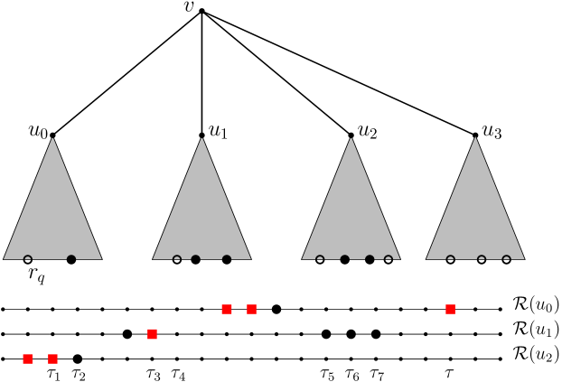
Figure 3: Illustration of $\textsc{FullUpdate}(v,\tau)$: leaves with filled dots are active and open dots are inactive, so ${\sf activesib}(u_{0},\tau)=\{u_{1},u_{2}\}$. The bold red squares or black circles denote timesteps in $\mathcal{R}(u)=\mathcal{R}^{s}(u)\cup\mathcal{R}^{ns}(u)$, with the red squares being awake at timestep $\tau$. Hence, $I_{u_{0}}=S_{u_{0}}=\varnothing$, $I_{u_{1}}=(\tau_{3},\tau],S_{u_{1}}=\{\tau_{4},\tau_{5},\tau_{6},\tau_{7}\},I_{u_{2}}=(\tau_{1},\tau],S_{u_{2}}=\{\tau_{2}\}.$ Timesteps in $\mathcal{R}^{s}(u)$ always remain awake.

For a constraint $C\in{\mathfrak{L}}^{u}(t)$, the variable $z_{C}$ is only raised in the call $\textsc{FullUpdate}(u,t)$. Subsequently, only the right side of (I3) can be raised. Hence, once a constraint $C$ becomes depleted, it stays depleted. It is worth discussing the special case when ${\sf activesib}(u_{0},\tau)$ is empty, so that $U=\{u_{0}\}$. In this case, no server transfer can happen, and the constraint $C(v,\sigma,\tau)$ is same as a slack constraint of $\mathfrak{L}^{u_{0}}(\tau)$, but with an additive term of $(n_{v}-n_{u_{0}})\delta$ on the RHS, as in (9). We still raise the dual variable $z_{C(v,\sigma,\tau)}$, and prove that the dual objective value rises by $\gamma$.

There is a parameter $M$ in line (3) that specifies the rate of change of $y^{v}$. This value $M$ should be an upper bound on the size of the index set $S_{u}$ over all calls to FullUpdate, and over all $u\in U$. Corollary 5.15 gives a bound of $M\leq\frac{5H\lambda^{H}k}{4\gamma}+1$, independent of the trivial bound $M\leq T$, where $T$ is the length of the input sequence.

5 Analysis Details

The proof rests on two lemmas: the first (proved in §5.1) bounds the movement cost in terms of the increase in dual value, and the second (proved in §5.2) shows near-feasibility of the dual solutions.

Lemma 5.1 (Server Movement).

The total movement cost during an execution of the procedure FullUpdate is at most $2\gamma$, and the objective value of the dual $\mathfrak{D}^{v}$ increases by exactly $\gamma$.

Lemma 5.2 (Dual Feasibility).

For each vertex $v$, the dual solution to $\mathfrak{L}^{v}$ is feasible if scaled down by a factor of $\beta$, where $\beta=O(\log\frac{nMk}{\gamma})=O(H\log(n\lambda))$.

Theorem 5.3 (Competitiveness for $k$-server).

Given any instance of the $k$-server problem on a $\lambda$-HST with height $H\leq\lambda/10$, Algorithm 1 ensures that each request location $\ell_{q}$ is saturated at some timestep in $[q,q+1)$. The total cost of (fractional) server movement is $O(\beta H)=O(H^{2}\log(n\lambda))$ times the cost of the optimal solution.

Proof.

All the server movement happens within calls to FullUpdate. By Lemma 5.1, each iteration of the while loop of line (1) in Algorithm 1 incurs a total movement cost of $O(H\gamma)$ over at most $H$ vertices on the backbone. Moreover, the call $\textsc{FullUpdate}(\mathbbm{r},\tau)$ corresponding to the root vertex $\mathbbm{r}$ increases the value of the dual solution to the LP $\mathfrak{L}^{\mathbbm{r}}$ by $\gamma$. This means the total movement cost is at most $O(H)$ times the dual solution value. Since all constraints of $\mathfrak{L}^{\mathbbm{r}}$ are implied by the relaxation $\mathfrak{M}$, any feasible dual solution gives a lower-bound on the optimal solution to $\mathfrak{M}$. By Lemma 5.2, the dual solution is feasible when scaled down by $\beta$, and so the (fractional) algorithm is $O(\beta H)=O(H^{2}\log(n\lambda))$-competitive. ∎

As mentioned in the introduction, using $\lambda$-HSTs with $\lambda=O(\log\Delta)$ allows us to extend this result to general metrics with a further loss of $O(\log^{2}\Delta)$.

5.1 Bounds on Server Transfer and Dual Increase

The dual increase of $\gamma$ claimed by Lemma 5.1 will follow from the proof of Invariant (I2). The upper bound on the server movement will follow from a new invariant, which we state below. Then in §5.1 we show both invariants are indeed maintained throughout the algorithm.

We first define the notion of the “lost” dual increase. Consider a call $\textsc{FullUpdate}(v,\tau)$. Let $u$ be $v$’s child such that request location $v_{0}$ lies in $T_{u}$. We say that $u$ is $v$’s principal child at timestep $\tau$. We prove (in Claim 5.11) that $\tau\in\mathcal{R}(u)$ remains in the awake set and hence $\tau_{u}=\tau$ throughout this procedure call. The dual update raises $z_{C(v,\sigma,\tau)}$ in line (3) and transfers servers from subtrees $T_{u^{\prime}}$ for $u^{\prime}\in{\sf activesib}(u,\tau)$ into subtree $T_{u}$ in line (3). This transfer has two components, which we consider separately. The first is the local component $\frac{dy^{v}(u,t)}{ds}$, and the second is the inherited component $\frac{b^{C_{u}}}{\lambda^{h}}$. In a sense, the inherited component matches the dual increase corresponding to the term $\sum_{u^{\prime}\in{\sf activesib}(u,\tau)}b^{C_{u^{\prime}}}$ on the RHS of (9). The only term without a corresponding server transfer is $b^{C_{u}}$ itself, where $C_{u}\in{\mathfrak{L}}^{u}(\tau)$ is the constraint in $\sigma$ corresponding to the principal child $u$. Motivated by this, we give the following definition.

Definition 5.4 (Loss).

For vertex $u$ with parent $v$, consider a timestep $\tau\in\mathcal{R}^{ns}(v)$ such that $\tau\in\mathcal{R}(u)$ as well. If $\tau\in\mathcal{R}^{s}(u)$, define ${\sf loss}(u,\tau):=0$. Else $\tau\in\mathcal{R}^{ns}(u)$, in which case.

$${\sf loss}(u,\tau):=\sum_{C\in{\mathfrak{L}}^{u}(\tau)}\;\sum_{C(v,\sigma,\tau):C\in\sigma}b^{C}\;z_{C(v,\sigma,\tau)}~{}~{}.$$ (10)

Invariant (I4).

For node $v$ and timestep $\tau\in\mathcal{R}^{ns}(v)$, let $u$ be $v$’s principal child at timestep $\tau$. The server mass entering subtree $T_{u}$ during the procedure $\textsc{FullUpdate}(v,\tau)$ is at most

$$\frac{\gamma-{\sf loss}(u,\tau)}{\lambda^{{\textsf{level}}(u)}}.$$ (I4)

Moreover, timestep $\tau\in\mathcal{R}(u)$ stays awake during the call $\textsc{FullUpdate}(v,\tau)$.

Multiplying the amount of transfer by the cost of this transfer, we get that the total movement cost is at most $O(\gamma)$. Invariants (I2) and (I4) prove Lemma 5.1. We now show these invariants hold over the course of the algorithm.

5.1.1 Proving Invariants (I2) and (I4)

To prove these invariants, we define a total order on pairs $(v,\tau)$ with $\tau\in\mathcal{R}(v)$ as follows:

$$\text{define: }(v_{1},\tau_{1})\prec(v_{2},\tau_{2})\text{ if }\tau_{1}<\tau_{2},\text{ or if $\tau_{1}=\tau_{2}$ and $v_{1}$ is a descendant of $v_{2}$}.$$

Since calls to FullUpdate are made in this order, we also prove the invariants by induction on this ordering: Assuming both invariants hold for all pairs $(v,\tau)\prec({v^{\star}},{\tau^{\star}})$, we prove them for the pair $({v^{\star}},{\tau^{\star}})$. The base case is easy to settle: at $q=0$, we only have $\bot$-constraints at the dummy leaf nodes. The only non-trivial statement among Invariants (I2) and (I4) for these nodes is to check that $b^{C}>0$ for any such $\bot$-constraint $C$ at a dummy leaf $v$. Note that $b^{C}=1-k_{v,0}-2\delta(n-1)=\frac{1}{2}-2\delta(n-1)>0$. DOuble-check this.

We start off with some supporting claims before proving the inductive step Invariants (I2) and (I4). First, we show that the notion of ${\sf prev}$ timestep in the FullUpdate procedure is well-defined.

Claim 5.5.

Let $u$ be any non-root vertex. Then the first timestep in $\mathcal{R}(u)$ corresponds to a $\bot$-constraint. Therefore, for any timestep $\tau$ such that $T_{u}$ has an active leaf at timestep $\tau$, ${\sf prev}(u,\tau)$ is well-defined.

Proof.

If $u$ is any of the dummy leaf nodes, then this follows by construction, the first timestep has a $\bot$-constraint. Else, let $q$ be the first time when a request arrives below $u$. Let $\tau_{f}$ be the first timestep after $q$. In the first iteration of the while loop in Algorithm 1 (corresponding to timestep $\tau_{f}$), we would call $\textsc{SimpleUpdate}(u,\tau_{f})$ because there are no active leaves below $u$ at this timestep. Hence we would add a $\bot$-constraint at timestep $\tau_{f}$, proving the first part of the claim. To show the second part, let $\tau$ be a timestep such that $T_{u}$ has an active leaf below it at timestep $\tau$. This means that $\tau\geq\tau_{f}$. Since $\mathfrak{L}^{u}(\tau_{f})$ is a $\bot$-constraint, $\tau_{f}$ is awake, and so ${\sf prev}(u,\tau)$ is well-defined. ∎

Next, we define ${\sf fill}(u,\tau)$ to to be the set of timesteps that load the constraints in $\mathfrak{L}^{u}(\tau)$. Formally, we have

Definition 5.6 (fill).

Given a node $u$ and its parent $v$, timestep $\tau\in\mathcal{R}^{ns}(u)$, and constraint $C\in{\mathfrak{L}}^{u}(\tau)$, define ${\sf fill}(C)$ to be the timesteps $\tau^{\prime}$ such that some constraint $C^{\prime}\in{\mathfrak{L}}^{v}(\tau^{\prime})$ appears on the RHS of inequality (I3) corresponding to $C$. All these timesteps $\tau^{\prime}$ must be after $\tau$. Extending this, let

$${\sf fill}(u,\tau):=\bigcup_{C\in{\mathfrak{L}}^{u}(\tau)}{\sf fill}(C).$$ (11)

In other words, ${\sf fill}(u,\tau)$ is the set of timesteps $\tau^{\prime}\in\mathcal{R}^{ns}(v)$ such that when we called $\textsc{FullUpdate}(v,\tau^{\prime}$), the node $u$ was either the $v$’s principal child at timestep $\tau^{\prime}$ or else belonged to the active sibling set, and moreover ${\sf prev}(u,\tau^{\prime})=\tau$. The following lemma shows part of their structure. Recall that $({v^{\star}},{\tau^{\star}})$ denotes the current pair in the inductive step.

Claim 5.7 (Structure of fill  times).

Fix a node $u$ with parent $v$, and a timestep $\tau\in\mathcal{R}^{ns}(u)$ such that $(v,\tau)\prec({v^{\star}},{\tau^{\star}})$. Then for any $\tau^{\prime}\in{\sf fill}(u,\tau)$, either (a) $\tau^{\prime}=\tau$, and $u$ is the principal child of $v$ at timestep $\tau^{\prime}$, or else (b) $\tau^{\prime}>\tau$, and $u$ is not $v$’s principal child at timestep $\tau^{\prime}$.

Proof.

Suppose $\tau=\tau^{\prime}$. Since we call FullUpdate only for ancestors of the requested node $v_{0}$, and $\tau\in\mathcal{R}^{ns}(u)$, so $v_{0}$ belongs to $T_{u}$ (and hence $u$ is the principal child of $v$ at timestep $\tau$). Else suppose $\tau^{\prime}>\tau$, and suppose $u$ is indeed $v$’s principal child at this timestep. Then during the call $\textsc{FullUpdate}(v,\tau^{\prime})$, we have ${\sf prev}(u,\tau^{\prime})=\tau^{\prime}$ throughout the execution of $\textsc{FullUpdate}(v,\tau^{\prime})$ (by the second statement in Invariant (I4)), and hence $\tau^{\prime}\notin{\sf fill}(u,\tau)$, giving a contradiction. ∎

We now give an upper bound on the server mass entering a subtree at any timestep $\tau<{\tau^{\star}}$.

Claim 5.8.

Let $\tau\in\mathcal{R}(u)$, $\tau<{\tau^{\star}}$. The server mass entering $T_{u}$ at timestep $\tau$ is at most

$$\left(1+\frac{1}{\lambda-1}\right)\frac{\gamma}{\lambda^{{\textsf{level}}(u)}}-\frac{{\sf loss}(u,\tau)}{\lambda^{{\textsf{level}}(u)}}.$$

Proof.

Since $\tau<{\tau^{\star}}$, we can apply the induction hypothesis to all pairs $(v,\tau)$ where $v$ is an ancestor of $u$. Servers enter $u$ at timestep $\tau$ because of $\textsc{FullUpdate}(w,\tau)$ for some ancestor $w$ of $u$. When $w$ is the parent of $u$, Invariant (I4) shows this quantity is at most $\frac{\gamma-{\sf loss}(u,\tau)}{\lambda^{h}},$ where $h={\textsf{level}}(u)$. For any other ancestor $w$ of $v$, Invariant (I4) implies a weaker upper bound of $\frac{\gamma}{\lambda^{h+k}}$, where ${\textsf{level}}(w)=h+k+1$. Simplifying the resulting geometric sum $\frac{\gamma-{\sf loss}(u,\tau)}{\lambda^{h}}+\sum_{h^{\prime}\geq h+1}\frac{\gamma}{\lambda^{h^{\prime}}}$ completes the proof. ∎

Next, we give a lower bound on the amount of server moving out of some subtree $T_{w}$. Such transfers out of $w$ takes place in line (3) with $w$ being either the node $u$ referred to on this line, or a descendant of such a node. Moreover, the server movement out of $T_{w}$ at timestep $\tau$ is denoted $g(w,\tau)$, which is non-zero only for those timesteps $\tau$ when $w$ is not on the corresponding backbone. We split this transfer amount into two:

• $g^{\mathsf{loc}}(w,\tau)$: the local component of the transfer, i.e., due to the increase in $y^{v}$ variables.

• $g^{\mathsf{inh}}(w,\tau)$: the inherited component of the transfer, i.e., due to the $b^{C_{u}}$ term.

Lemma 5.9.

Let $u$ be a non-principal child of ${v^{\star}}$ at timestep ${\tau^{\star}}$, and $I:=(\tau_{1},{\tau^{\star}}]$ for some timestep $\tau_{1}<{\tau^{\star}}$. Let $S$ be the timesteps in $\mathcal{R}^{ns}(u)\cap(\tau_{1},{\tau^{\star}}]$ that have been removed from ${\sf Awake}(u)$ by the moment when $\textsc{FullUpdate}({v^{\star}},{\tau^{\star}})$ is called. Then

$$g^{\mathsf{inh}}(u,(\tau_{1},{\tau^{\star}}])\geq\left(1+\frac{1}{H}\right)|S|\,\frac{\gamma}{\lambda^{{\textsf{level}}(u)}}-\sum_{\tau\in S}\frac{{\sf loss}(u,\tau)}{\lambda^{{\textsf{level}}(u)}}.$$

Proof.

Consider timesteps $\tau\in S$ and $\tau^{\prime}\geq\tau$ such that $\tau^{\prime}\in{\sf fill}(u,\tau)$. (We use the term phase here to denote a range of values of the timer $s$.) Consider the phase during $\textsc{FullUpdate}({v^{\star}},\tau^{\prime})$ when $\tau_{u}^{\prime}:={\sf prev}(u,\tau^{\prime})$ equals $\tau$: since $\tau^{\prime}\in{\sf fill}(u,\tau)$, we know that there will be such a phase. Whenever we raise the timer $s$ by a small $\varepsilon$ amount during this phase, we raise some dual variable $z_{C({v^{\star}},\sigma,\tau^{\prime})}$ by the same amount, where $\sigma$ contains a constraint $C$ from ${\mathfrak{L}}^{u}(\tau)$. Thus we contribute $\varepsilon$ to the LHS of (I3) for constraint $C$. For such a constraint $C$, let $[s_{1}(\tau^{\prime},C),s_{2}(\tau^{\prime},C)]$ be the range of the timer $s$ during which we raise a dual variable of the form $z_{C({v^{\star}},\sigma,\tau^{\prime})}$ such that $C\in\sigma$.

The timestep $\tau$ was removed from ${\sf Awake}(u)$ by line (3) because (I3) became tight for all constraints $C\in{\mathfrak{L}}^{u}(\tau)$, so:

$$\left(1+\frac{1}{H}\right)\sum_{C\in{\mathfrak{L}}^{u}(\tau)}b^{C}z_{C} =\sum_{C\in{\mathfrak{L}}^{u}(\tau)}b^{C}\sum_{C({v^{\star}},\sigma,\tau^{\prime}):C\in\sigma}z_{C({v^{\star}},\sigma,\tau^{\prime})}$$

Now the definition of $${\sf loss}(u,\tau)$$ allow us to split the expression on the RHS as follows:

$$={\sf loss}(u,\tau)+\sum_{C\in{\mathfrak{L}}^{u}(\tau)}b^{C}\sum_{C({v^{\star}},\sigma,\tau^{\prime}):C\in\sigma,\tau^{\prime}>\tau}z_{C({v^{\star}},\sigma,\tau^{\prime})}$$

$$={\sf loss}(u,\tau)+\sum_{\tau^{\prime}\in{\sf fill}(u,\tau),\tau^{\prime}>\tau}\sum_{C\in{\mathfrak{L}}^{u}(\tau)}b^{C}\Big{(}s_{2}(\tau^{\prime},C)-s_{1}(\tau^{\prime},C)\Big{)}.$$ (12)

We now bound the second expression on the RHS in another way. For a timestep $\tau^{\prime}\in{\sf fill}(u,\tau)$ with $\tau^{\prime}>\tau$, consider the phase when timer $s$ lies in the range $[s_{1}(\tau^{\prime},C),s_{2}(\tau^{\prime},C)]$ for a constraint $C\in{\mathfrak{L}}^{u}(\tau)$. Since $\tau^{\prime}>\tau$, Claim 5.7 implies that $u$ is not the principal child of ${v^{\star}}$ at timestep $\tau^{\prime}$, so raising $s$ by $\varepsilon$ units during this phase means that line (3) moves $\varepsilon\cdot\frac{b^{C}}{\lambda^{h}}$ servers out of $T_{u}$, where $h:={\textsf{level}}(u)$. Hence the increase in $g^{\mathsf{inh}}(u,I)$ due to transfers corresponding to timestep $\tau\in S$ is at least

$$\sum_{\tau^{\prime}\in{\sf fill}(u,\tau),\tau^{\prime}>\tau}\sum_{C\in{\mathfrak{L}}^{u}(\tau)}\frac{b^{C}(s_{2}(\tau^{\prime},C)-s_{1}(\tau^{\prime},C))}{\lambda^{h}} ~{}~{}\stackrel{{\scriptstyle\text{by~{}\eqref{eq:calc1}}}}{{=}}~{}~{}\left(1+\frac{1}{H}\right)\sum_{C\in{\mathfrak{L}}^{u}(\tau)}\frac{b^{C}z_{C}}{\lambda^{h}}-\frac{{\sf loss}(u,\tau)}{\lambda^{h}}$$

$$=\left(1+\frac{1}{H}\right)\frac{\gamma}{\lambda^{h}}-\frac{{\sf loss}(u,\tau)}{\lambda^{h}}.$$

The final equality above uses $(u,\tau)\prec({v^{\star}},{\tau^{\star}})$, because $\tau$ had been removed from ${\sf Awake}(u)$ before the call to $\textsc{FullUpdate}({v^{\star}},{\tau^{\star}})$, which means we can use the induction hypothesis Invariant (I2) for timestep $\tau\in\mathcal{R}^{ns}(u)$. Finally, summing over all timesteps in $S$ completes the proof. ∎

Corollary 5.10.

Let $u$ be a non-principal child of ${v^{\star}}$ at timestep ${\tau^{\star}}$, and $I:=(\tau_{1},{\tau^{\star}}]$. Consider the moment when $\textsc{FullUpdate}({v^{\star}},{\tau^{\star}})$ is called. If none of the timesteps in $I\cap\mathcal{R}(u)$ belong to ${\sf Awake}(u)$, then

• $g^{\mathsf{inh}}(u,I)\geq r(u,I)$,

• $0\leq g^{\mathsf{loc}}(u,I)\leq D(u,I)$, and

• $g^{\mathsf{loc}}(u,I)\geq y^{{v^{\star}}}(u,I)$.

Finally, $b^{C}>0$ for any constraint $C\in\mathfrak{L}^{v^{\star}}({\tau^{\star}})$ of the form $a^{C}\cdot y^{v}\geq b^{C}$.

Proof.

Since timesteps in $\mathcal{R}^{s}(u)$ always stay awake, $I\cap\mathcal{R}(u)=I\cap\mathcal{R}^{ns}(u)$; call this set $S$. Since $u$ is a non-principal child at timestep ${\tau^{\star}}$, we have ${\tau^{\star}}\not\in\mathcal{R}^{ns}(u)$. This means $\tau<{\tau^{\star}}$ for any $\tau\in S$, and so Claim 5.8 gives an upper bound on the server movement into $u$ at timestep $\tau$, and Lemma 5.9 gives a lower bound on the server movement out of $u$. Combining the two,

$$g^{\mathsf{inh}}(u,I)-r(u,I)\geq\left(\frac{1}{H}-\frac{1}{\lambda-1}\right)\frac{\gamma|S|}{\lambda^{h}}\geq\frac{4}{5H}\cdot\frac{\gamma|S|}{\lambda^{h}}\geq 0,$$ (13)

since $\lambda\geq 10H$ and $H\geq 2$, which proves (i). To prove (ii),

$$g^{\mathsf{loc}}(u,I)=(g-g^{\mathsf{inh}})(u,I)\stackrel{{\scriptstyle\text{by~{}(i)}}}{{\leq}}(g-r)(u,I)\stackrel{{\scriptstyle\text{by defn.}}}{{=}}D(u,I).$$

To prove (iii), whenever we raised $y^{{v^{\star}}}(u,\tau^{\prime})$ for some timestep $\tau^{\prime}$, we raised $g^{\mathsf{loc}}(u,\tau^{\prime\prime})$ for some $\tau^{\prime\prime}\geq\tau^{\prime}$) with the same rate. Both timesteps $\tau^{\prime},\tau^{\prime\prime}$ appear before ${\tau^{\star}}$, because we consider the moment when we call $\textsc{FullUpdate}({v^{\star}},{\tau^{\star}})$. Since interval $I$ ends at ${\tau^{\star}}$, it must contain either only $\tau^{\prime\prime}$ or both $\tau^{\prime},\tau^{\prime\prime}$, giving us that $g^{\mathsf{loc}}(u,I)\geq y^{{v^{\star}}}(u,I)$.

$\ll$Anupam 5.1: Stopping here.$\gg$ We now prove the final statement. If $C\in\mathfrak{L}^{v^{\star}}({\tau^{\star}})$ is a $\bot$-constraint $C$ added by $\textsc{SimpleUpdate}({v^{\star}},{\tau^{\star}})$. $b^{C}=1-k_{{v^{\star}},{\tau^{\star}}}-2\delta(n-n_{v^{\star}})$ (using (4)). Since $k_{{v^{\star}},{\tau^{\star}}}\leq 1-\delta^{\prime}$ (otherwise the while loop in Algorithm 1 would have terminated), we see that $b^{C}\geq\delta^{\prime}-2\delta n>0$. The other case is when $C$ is of the form $C({v^{\star}},\sigma,{\tau^{\star}})$ as in (9). By the induction hypothesis (Invariant (I2)), $b^{C_{u}}>0$ and $D(u,I_{u})\geq 0$ by (ii) above. Since $n_{v^{\star}}>\sum_{u\in U}n_{u}$, it follows that $b^{C}>0$. ∎

Having proved all the supporting claims, we start off with proving that the second statement in Invariant (I2) holds at $({v^{\star}},{\tau^{\star}})$.

Claim 5.11 (Principal Node Awake).

Suppose we call $\textsc{FullUpdate}({v^{\star}},{\tau^{\star}})$. If $u$ is the principal child of ${v^{\star}}$ at timestep ${\tau^{\star}}$, this call does not remove the timestep ${\tau^{\star}}$ from ${\sf Awake}(u)$.

Proof.

At the beginning of the call to $\textsc{FullUpdate}({v^{\star}},{\tau^{\star}})$, the timestep ${\tau^{\star}}$ has just been added to $\mathcal{R}(u)$ (and to ${\sf Awake}(u)$) in the call to $\textsc{FullUpdate}(u,{\tau^{\star}})$ or to $\textsc{SimpleUpdate}(u,{\tau^{\star}})$, and cannot yet be removed from ${\sf Awake}(u)$. So we start with $\tau_{u}={\tau^{\star}}$. For a contradiction, if we remove ${\tau^{\star}}$ from ${\sf Awake}(u)$ in line (3), then all the constraints in ${\mathfrak{L}}^{u}({\tau^{\star}})$ must have become depleted. For each such constraint $C\in{\mathfrak{L}}^{u}({\tau^{\star}})$, the contributions to the RHS in (I3) during this procedure come only from the newly-added constraints $C({v^{\star}},\sigma,{\tau^{\star}})\in{\mathfrak{L}}^{v^{\star}}({\tau^{\star}})$. So if all constraints in ${\mathfrak{L}}^{u}({\tau^{\star}})$ become depleted, the total dual objective raised during this procedure is at least

$$\sum_{C\in{\mathfrak{L}}^{u}({\tau^{\star}})}\;\sum_{C({v^{\star}},\sigma,{\tau^{\star}})\in{\mathfrak{L}}^{v^{\star}}({\tau^{\star}}):C\in\sigma}b^{C({v^{\star}},\sigma,{\tau^{\star}})}\;z_{C({v^{\star}},\sigma,{\tau^{\star}})}\geq\left(1+\nicefrac{{1}}{{H}}\right)\sum_{C\in{\mathfrak{L}}^{u}({\tau^{\star}})}b^{C}\,z_{C},$$

where we use that $b^{C({v^{\star}},\sigma,{\tau^{\star}})}\geq b^{C}$ (because in (9), $b^{C_{u}}\geq 0$ by the induction hypothesis (Invariant (I2)) and $D(u,I_{u})\geq 0$ by Corollary 5.10), and that each constraint in ${\mathfrak{L}}^{u}({\tau^{\star}})$ satisfies (I3) at equality. The induction hypothesis Invariant (I2) applied to $(u,{\tau^{\star}})$ implies that $\sum_{C\in{\mathfrak{L}}^{u}({\tau^{\star}})}b^{C}\,z_{C}=\gamma$, so the RHS above is $(1+\nicefrac{{1}}{{H}})\gamma$. So the total dual increase during $\textsc{FullUpdate}({v^{\star}},{\tau^{\star}})$, which is at least the LHS above, is strictly more than $\gamma$, contradicting the stopping condition of $\textsc{FullUpdate}({v^{\star}},{\tau^{\star}})$. ∎

Next, we prove the remainder of the inductive step, namely that Invariants (I2) and (I4) are satisfied with respect to $({v^{\star}},{\tau^{\star}})$ as well.

Claim 5.12 (Inductive Step: Active Siblings Exist).

Consider the call $\textsc{FullUpdate}({v^{\star}},{\tau^{\star}})$, and let $u_{0}$ be the principal child of ${v^{\star}}$ at this timestep. Suppose ${\sf activesib}(u_{0},{\tau^{\star}})\neq\varnothing$. Then the dual objective value corresponding to the constraints in ${\mathfrak{L}}^{v^{\star}}({\tau^{\star}})$ equals $\gamma$; i.e.,

$$\sum_{C\in{\mathfrak{L}}^{v^{\star}}({\tau^{\star}})}z_{C}\,b^{C}=\gamma.$$

Moreover, the server mass entering $T_{u_{0}}$ going to the requested node in this call is at most

$$\frac{\gamma-{\sf loss}(u_{0},{\tau^{\star}})}{\lambda^{{\textsf{level}}(u)}}.$$

Proof.

Let $U^{\prime}:={\sf activesib}(u_{0},{\tau^{\star}})$ be the non-principal children of ${v^{\star}}$ at timestep ${\tau^{\star}}$; let $U:=\{u_{0}\}\cup U^{\prime}$ as in FullUpdate. The identity of the timesteps $\tau_{u}$ and intervals $I_{u}$ change over the course of the call, so we need notation to track them carefully. Let $I_{u}(s^{\prime})$ be the set $I_{u}$ when the timer value is $s^{\prime}$; similarly, let $D_{s}(u,I_{u}(s^{\prime}))$ be the value of $D(u,I_{u}(s^{\prime}))$ when the timer value is $s$, and $y^{{v^{\star}}}_{s}(u,I_{u}(s^{\prime}))$ is defined similarly.

For $u\in U^{\prime}$, Corollary 5.10(ii,iii) implies that for any interval $I_{u}(s)$,

$$D_{0}(u,I_{u}(s))\geq y^{{v^{\star}}}_{0}(u,I_{u}(s)).$$ (14)

Since the timestep ${\tau^{\star}}$ stays awake for the principal child $u_{0}$ (due to Claim 5.11), the interval $I_{u_{0}}(s)$ equals $({\tau^{\star}},{\tau^{\star}}]$, which is empty, for all values of the timer $s$.

The dual increase is at most $\gamma$ due to the stopping criterion for FullUpdate, so we need to show this quantity reaches $\gamma$. Indeed, suppose we raise the timer from $s$ to $s+ds$ when considering some constraint $C_{s}(v,\sigma,\tau)$—the subscript indicates the constraint considered at that value of timer $s$. The dual objective increases by $b^{C_{s}(v,\sigma,\tau)}\,ds$. We now use the definition of $b^{C_{s}(v,\sigma,\tau)}$ from (9), substitute $(n_{v}-\sum_{u\in U}n_{u})\geq 1$, and use that all $b^{C_{u}}$ terms in the summation are non-negative (by Invariant (I2)) to drop these terms. This gives the first inequality below (recall that $I_{u_{0}}(s)$ stays empty):

$$b^{C_{s}(v,\sigma,\tau)} \geq\sum_{u\in U^{\prime}}D_{s}(u,I_{u}(s))+\delta\geq\sum_{u\in U^{\prime}}D_{0}(u,I_{u}(s))+\delta\geq\sum_{u\in U^{\prime}}y^{{v^{\star}}}_{0}(u,I_{u}(s))+\delta.$$ (15)

The second inequality above uses that $D_{s}\geq D_{0}$ for non-principal children, and the third uses (14). Let

$$Y(s):=\sum_{\tau^{\prime}}\sum_{u\in U^{\prime}}\Big{(}y^{{v^{\star}}}_{s}(u,\tau^{\prime})-y^{{v^{\star}}}_{0}(u,\tau^{\prime})~{}\Big{)}$$

to be the total increase in the $y^{{v^{\star}}}$ variables during $\textsc{FullUpdate}({v^{\star}},{\tau^{\star}})$ until the timer reaches $s$. This is also the total amount of server transferred to the requested node due to the local component of transfer in line (3) until this moment.

Subclaim 5.13.

$Y(s)<\gamma$.

Proof.

Suppose not, and let $s^{\star}$ be the smallest value of the timer such that $Y(s^{\star})=\gamma$. Note that $Y(s)$ is a continuous non-decreasing function of $s$. For any $s\in[0,s^{\star})$, we get $Y(s)<Y(0)+\gamma$, where $Y(0)=0$ by definition. Since the intervals $I_{u}(s^{\prime})\subseteq I_{u}(s)$ for $s^{\prime}\leq s$, all the increases in the $y^{{v^{\star}}}$ variables during $[0,s]$ correspond to timesteps in $I_{u}(s)$. Thus for any $s<s^{\star}$,

$$Y(0)+\gamma>Y(s)\quad\implies\quad\sum_{u\in U^{\prime}}y^{{v^{\star}}}_{0}(u,I_{u}(s))+\gamma>\sum_{u\in U^{\prime}}y^{{v^{\star}}}_{s}(u,I_{u}(s)).$$ (16)

The dual increase during $[s,s+ds]$ is

$$b^{C_{s}(v,\sigma,\tau)}\,ds \stackrel{{\scriptstyle\text{by~{}(\ref{eq:transy},\ref{eq:YY})}}}{{>}}\Big{(}\sum_{u\in U^{\prime}}y^{{v^{\star}}}_{s}(u,I_{u}(s))+\delta-\gamma\Big{)}\,ds$$

$$=\Big{(}\lambda^{h}\,dY(s)-\frac{\gamma}{Mn}\sum_{u\in U^{\prime}}|S_{u}|\,ds\Big{)}+(\delta-\gamma)\,ds>\lambda^{h}\,dY(s)\geq dY(s).$$

The second line uses (a) the update rule in line (3) with $dY(s)$ denoting $Y(s+ds)-Y(s)$, (b) that $M\geq|S_{u}|$ and $|U^{\prime}|\leq n$, so the second expression is bounded by $\gamma$, and (c) that $\delta>2\gamma$. Integrating over $[0,s^{\star}]$, the total dual increase is strictly more than $Y(s^{\star})=\gamma$, which contradicts the stopping condition of FullUpdate. ∎

Combining Subclaim 5.13 (and specifically its implication (16)) with (14) implies that for all values $s$ of the timer:

$$\sum_{u\in U^{\prime}}y^{{v^{\star}}}_{s}(u,I_{u}(s))<\sum_{u\in U^{\prime}}D_{0}(u,I_{u}(s))+\gamma.$$ (17)

Therefore, the increase in dual objective during $[s,s+ds]$ is at least

$$b^{C_{s}(v,\sigma,\tau)}\,ds \stackrel{{\scriptstyle\eqref{eq:cons}}}{{\geq}}\bigg{(}\sum_{u\in U^{\prime}}\Big{(}D_{0}(u,I_{u}(s))+b^{C_{u,s}}\Big{)}+\delta+b^{C_{u_{0}}}\bigg{)}\,ds$$

$$\stackrel{{\scriptstyle\eqref{eq:timery1}}}{{>}}\bigg{(}\sum_{u\in U^{\prime}}\Big{(}y^{{v^{\star}}}_{s}(u,I_{u}(s))+b^{C_{u,s}}\Big{)}+(\delta-\gamma)+b^{C_{u_{0}}}\bigg{)}\,ds$$

$$\geq\sum_{u\in U^{\prime}}\Big{(}\lambda^{h}\,dy^{{v^{\star}}}_{s}(u,I_{u}(s))-\frac{\gamma}{Mn}|S_{u}|\,ds+b^{C_{u,s}}\,ds\Big{)}+\gamma\,ds+b^{C_{u_{0}}}\,ds$$

$$\geq\sum_{u\in U^{\prime}}\Big{(}\lambda^{h}\,dy^{{v^{\star}}}_{s}(u,I_{u}(s))+b^{C_{u,s}}\Big{)}\,ds+b^{C_{u_{0}}}\,ds$$

$$=\lambda^{h}[\text{amount of server transferred in $[s,s+ds]$}]+b^{C_{u_{0}}}\,ds$$

Here $C_{u,s}$ is the constraint corresponding to $u\in U^{\prime}$ when the timer equals $s$. The third inequality above follows from the update rule in line (3), and that $\delta\geq 2\gamma$. The last equality follows from line (3). Integrating over the entire range of the timer $s$, we see that the total dual objective increase is at least $\lambda^{h}[\text{total server transfer}]+{\sf loss}(u_{0},{\tau^{\star}})$. Since the total dual increase is at most $\gamma$, the total server transfer is at most $\frac{\gamma-{\sf loss}(u_{0},{\tau^{\star}})}{\lambda^{h}}$. This proves the second part of Claim 5.12.

We now prove that the FullUpdate process does not stop until the dual increase is $\gamma$. For each $u\in U^{\prime}$, the subtree $T_{u}$ contains at least one active leaf and hence at least $\delta$ servers when FullUpdate is called. Since the total server transfer is at most $\gamma\ll\delta$, we do not run out of servers. It follows that until the dual objective reaches $\gamma$, we keep raising $y^{{v^{\star}}}_{s}(u,I_{u}(s))$ for some non-empty interval $I_{u}(s)$ for each $u\in U^{\prime}$, and this also raises the dual objective as above. ∎

It remains to consider the general case when ${\sf activesib}(u_{0},{\tau^{\star}})$ may be empty.

Claim 5.14 (Inductive Step: General Case).

At the end of any call $\textsc{FullUpdate}({v^{\star}},{\tau^{\star}})$, the total dual objective raised during the call equals $\gamma$.

Proof.

If ${\sf activesib}(u_{0},{\tau^{\star}})$ is non-empty, this follows from Claim 5.12. So assume that ${\sf activesib}(u_{0},{\tau^{\star}})$ is empty. In this case, there are no $y^{v}(u,t)$ variables to raise because the interval $I_{u_{0}}$ is empty. As we raise $s$, we also raise $z_{C({v^{\star}},\sigma,{\tau^{\star}})}$ in line (3). Since we do not make all the constraints in ${\mathfrak{L}}^{u_{0}}({\tau^{\star}})$ depleted (Claim 5.14), the total dual increase must reach $\gamma$, because $b^{C({v^{\star}},\sigma,{\tau^{\star}})}>0$ by Corollary 5.10. ∎

This completes the proof of the induction hypothesis for the pair $({v^{\star}},{\tau^{\star}})$. Before we show dual feasibility, we give an upper bound on the parameter $M$.

Corollary 5.15 (Bound on $M$).

For node $u$ and timestep $\tau$, let $\tau_{u}:={\sf prev}(u,\tau)$. There are at most $\frac{5H\lambda^{H}k}{4\gamma}+1$ timesteps in $(\tau_{u},\tau]\cap\mathcal{R}^{ns}(u)$. So we can set $M$ to $\frac{5H\lambda^{H}k}{4\gamma}+1$.

Proof.

Let $I:=(\tau_{u},\tau]$. By the choice of $\tau_{u}$, none of the timesteps in $S:=I\cap\mathcal{R}^{ns}(u)$ belong to ${\sf Awake}(u)$. The proof of Corollary 5.10, and specifically (13), shows that $g^{\mathsf{inh}}(u,I)-r(u,I)\geq\frac{4|S|\gamma}{5H\lambda^{h}}$. This difference cannot be more than the total number of servers, so $|S|\leq\frac{5H\lambda^{H}k}{4\gamma}$. Since the set $|S_{u}|$ defined in line 3 in FullUpdate is at most $|S|+1$ (because of the first timestep of $I_{u}$), the desired result follows. ∎

5.2 Approximate Dual Feasibility

For $\beta\geq 1$, a dual solution $z$ is $\beta$-feasible if $z/\beta$ satisfies satisfies the dual constraints. We now show that the dual variables raised during the calls to $\textsc{FullUpdate}(v,\tau)$ for various timesteps $\tau$ remain $\beta$-feasible for $\beta=O(\ln\frac{nMk}{\gamma})$. First we show Invariant (I1), and also give bounds on variables $y^{v}(u,t)$.

Claim 5.16 (Proof of Invariant (I1)).

For any timestep $\tau$ and leaf $v$, the server amount $k_{v,\tau}$ remains in the range $[\nicefrac{{\delta}}{{2}},1-\nicefrac{{\delta^{\prime}}}{{2}}]$.

Proof.

Recall that $\gamma\leq 4\delta\ \leq 4\delta^{\prime}$. Lemma 5.1 proves that the total server mass entering the request location in any timestep is at most $2\gamma$. Since the request location must have less than $1-\delta^{\prime}$ at the start of the timestep, $k_{v,\tau}$ remains at most $1-\delta^{\prime}+2\gamma\leq 1-\nicefrac{{\delta^{\prime}}}{{2}}$. Similarly, we move server mass from a leaf only when it is active, i.e., has at least $\delta$ server mass. Hence, $k_{v,\tau}$ remains at least $\delta-2\gamma\geq\nicefrac{{\delta}}{{2}}$. ∎

Claim 5.17 (Bound on $y^{v}$ Values).

For any vertex $v$, any child $u$ of $v$, and timestep $\tau$, the variable $y^{v}(u,\tau)\leq 4\gamma M+k$.

Proof.

For a contradiction, consider a call $\textsc{FullUpdate}(v,\tau^{\prime})$ during which we are about to raise $y^{v}(u,\tau)$ beyond $4\gamma M+k$. Any previous increases to $y^{v}(u,\tau)$ happen during calls $\textsc{FullUpdate}(v,\tau^{\prime\prime})$ for some $\tau^{\prime\prime}\in[\tau,\tau^{\prime}]$. Moreover, whenever we raise $y^{v}(u,\tau)$ by some amount, we move out at least the same amount of server mass from the subtree $T_{u}$. Hence, at least $4\gamma M+k$ amount of server mass has been moved out of $T_{u}$ in the interval $[\tau,\tau^{\prime}]$. Since we have a non-negative amount of server in $T_{u}$ at all times, we must have moved in at least $4\gamma M$ amounts of server into $T_{u}$ during the same interval. All this movement happens at timesteps in $\mathcal{R}(u)$. Moreover, for each individual timestep $\tau^{\prime\prime}\in\mathcal{R}(u)$, we bring at most $2\gamma$ servers into $T_{u}$, so there must be at least $2M$ timesteps in $\mathcal{R}(u)\cap[\tau,\tau^{\prime}]$. Finally, since we are raising $y^{v}(u,\tau)$ at timestep $\tau^{\prime}$, the interval $I_{u}$ (defined in line (3)) at timestep $\tau^{\prime}$ must contain $[\tau,\tau^{\prime}]$, which means $|I_{u}\cap\mathcal{R}^{ns}(u)|>M$ (because no timestep in $\mathcal{R}^{s}(u)$ can lie in $[\tau,\tau^{\prime}]$). This contradicts the definition of $M$. ∎

Claim 5.18.

Let $t$ be any timestep typo: in $\mathcal{R}(u)$, and $v$ be the parent of $u$. Define $t_{1}$ to be the last timestep in $\mathcal{R}(u)\cap[0,t]$, and $t_{2}$ to be the next timestep, i.e., $t_{1}+\eta$. Let $C$ be a constraint in $\mathfrak{L}^{v}$ containing the variable $y^{v}(u,t)$ on the LHS. Then $C$ contains at least one of $y^{v}(u,t_{1})$ and $y^{v}(u,t_{2})$. Moreover, whenever we raise $z(C)$ in line (3) of the FullUpdate procedure, we also raise either $y^{v}(u,t_{1})$ or $y^{v}(u,t_{2})$ according to line (3).

Proof.

Suppose $y^{v}(u,t)$ appears in a constraint $\mathfrak{L}^{v}(\tau)$. Define $I_{u}=(\tau_{u},\tau]$ as in line (3). It follows that $t\in I_{u}$, and so $\tau_{u}<t$. Therefore, $\tau_{u}\in\mathcal{R}(u)\cap[0,t]$, so either $t_{1}>\tau_{u}$ and hence belongs to $I_{u}$, or else $t_{1}=\tau_{u}$ in which case $t_{2}\in I_{u}$. It follows that the index set $S_{u}$ contains either $t_{1}$ or $t_{2}$. This implies the second statement in the claim. ∎

We now show the approximate dual feasibility. Recall that the constraints added to ${\mathfrak{L}}^{v}(\tau)$ are of the form $C(v,\sigma,\tau)$ given in (9), and we raise the corresponding dual variable $z_{C(v,\sigma,\tau)}$ only during the procedure $\textsc{FullUpdate}(v,\tau$) and never again.

Lemma 5.19 (Approximate Dual Feasibility).

For a node $v$ at height $h+1$, the dual variables $z_{C}$ are $\beta_{h}$-feasible for the dual program $\mathfrak{D}^{v}$, where $\beta_{h}=\left(1+\nicefrac{{1}}{{H}}\right)^{h}O(\ln n+\ln M+\ln(k/\gamma)).$

Proof.

We prove the claim by induction on the height of $v$. For a leaf node, this follows vacuously, since the primal/dual programs are empty. Suppose the claim is true for all nodes of height at most $h$. For a node $v$ at height $h+1>0$ with children $\chi_{v}$, the variables in ${\mathfrak{L}}^{v}$ are of two types: (i) $y^{v}(u,t)$ for some timestep $t$ and child $u\in\chi_{v}$, and (ii) $y^{v}(u^{\prime},t)$ for some timestep $t$ and non-child descendant $u^{\prime}\in T_{v}\setminus\chi_{v}$. We consider these cases separately:

1. Suppose the dual constraint corresponds to variable $y^{v}(u,t)$ for some child $u\in\chi_{v}$. Let ${\mathfrak{L}}^{\prime}$ be the set of constraints in ${\mathfrak{L}}^{v}$ containing $y^{v}(u,t)$ on the LHS. The dual constraint is:

   $$\sum_{C\in{\mathfrak{L}}^{\prime}}z_{C}\leq c_{u}=\lambda^{h}.$$ (18)

   Let $t_{1},t_{2}$ be as in the statement of Claim 5.18. When we raise $z_{C}$ for a constraint $C\in{\mathfrak{L}}^{\prime}$ in line (3) at unit rate, we raise either $y^{v}(u,\tau_{1})$ or $y^{v}(u,t_{2})$ at the rate given by line (3). Therefore, if we raise the LHS of the dual constraint (18) for a total of $\Gamma$ units of the timer, we would have raised one of the two variables, say $y^{v}(u,\tau_{1})$, for at least $\Gamma/2$ units of the timer. Therefore, the value of $y^{v}(u,\tau_{1})$ variable due to this exponential update is at least

   $$\frac{\gamma}{Mn}(e^{\Gamma/2\lambda^{h}}-1).$$

   By Claim 5.17, this is at most $4\gamma M+k$, so we get

   $$\Gamma=\lambda^{h}\cdot O\left(\ln n+\ln M+\ln(k/\gamma)\right)=\beta_{0}c_{u},$$

   hence showing that (18) is satisfied up to $\beta_{0}$ factor.

2. Suppose the dual constraint corresponds to some variable $y^{v}(u^{\prime},\tau)$ with $u^{\prime}\in T_{u}$, and $u\in\chi_{v}$. Suppose $u^{\prime}$ is a node at height $h^{\prime}<h$. Now let ${\mathfrak{L}}^{\prime}$ be the constraints in ${\mathfrak{L}}^{u}$ (the LP for the child $u$) which contain $y^{u}(u^{\prime},\tau)$. By the induction hypothesis:

   $$\sum_{C\in{\mathfrak{L}}^{\prime}}z_{C}\leq\beta_{h-1}\;c_{u^{\prime}}.$$ (19)

   Let ${\mathfrak{L}}^{\prime\prime}$ denote the set of constraints in ${\mathfrak{L}}^{v}$ (the LP for the parent $v$) which contain $y^{v}(u^{\prime},\tau)$. Each constraint $C(v,\sigma,\tau)$ in this set ${\mathfrak{L}}^{\prime\prime}$ has the coordinate $\sigma_{u}$ corresponding to the child $u$ being a constraint in ${\mathfrak{L}}^{\prime}$, which implies:

   $$\sum_{C(v,\sigma,\tau)\in{\mathfrak{L}}^{\prime\prime}}z_{C(v,\sigma,\tau)}=\sum_{C\in{\mathfrak{L}}^{\prime}}\sum_{C(v,\sigma,\tau)\in{\mathfrak{L}}^{\prime\prime}:\sigma_{u}=C}z_{C(v,\sigma,\tau)}\leq(1+\nicefrac{{1}}{{H}})\;\sum_{C\in{\mathfrak{L}}^{\prime}}z_{C},$$ (20)

   where the last inequality uses Invariant (I3). Now the induction hypothesis (19) and the fact that $\beta_{h}=(1+\nicefrac{{1}}{{H}})\,\beta_{h-1}$ completes the proof. ∎

Lemma 5.19 means that the dual solution for ${\mathfrak{L}}^{\mathbbm{r}}$ is $\beta_{H}$-feasible, where $\beta_{H}=O(\ln\frac{nMk}{\gamma})$. This proves Lemma 5.2 and completes the proof of our fractional $k$-server algorithm.

6 Algorithm for $k$-ServerTW

In this section, we describe the online algorithm for $k$-ServerTW. The structure of the algorithm remains similar to that for $k$-Server. Again, we have a main procedure (Algorithm 4) which considers the backbone consisting of the path from the requested leaf node to the root node. It calls a suitable subroutine for each node on this backbone to add local LP constraints and/or transfer servers to $v_{0}$. We say that a request interval $R_{q}=[b,q]$ at a leaf node $\ell_{q}$ becomes critical (at time $q$) if it has deadline $q$, and it has not been served until time $q$, i.e., if $k_{\ell_{q},t}<1-2\delta^{\prime}$ for all timesteps $t\in[b,q)$: for technical reasons we allow a gap of up to $2\delta^{\prime}$ instead of $\delta^{\prime}$. In case this node becomes critical at $q$, the algorithm ensures that $\ell_{q}$ receives at least $1-\delta^{\prime}$ amount of server at time $q$. This ensures that we move at least $\delta^{\prime}$ amount of server mass when a request becomes critical. The parameters $\delta,\delta^{\prime}$ remain unchanged, but we set $\gamma$ to $\frac{1}{n^{4}\Delta}$. We extend the definition of ReqLoc from §4 in the natural way:

$$\textsf{ReqLoc}(\tau)=\text{location of request with deadline at time $\lfloor\tau\rfloor$, and }$$

$$\operatorname{\textsf{ReqInt}}(\tau)=\text{request interval with deadline at time $\lfloor\tau\rfloor$}.$$

0.1 foreach $q=1,2,\ldots$ do

0.2       if $\operatorname{\textsf{ReqInt}}(q)$ exists and is critical  then

0.3             let the path from $\ell_{q}:=\textsf{ReqLoc}(q)$ to the root be $\ell_{q}=v_{0},v_{1},\ldots,v_{H}=\mathbbm{r}$.;

0.4             let $Z_{q},\{F_{v,q}\mid v\in Z_{q}\}\leftarrow{\textsc{BuildTree}}(q)$ ;

0.5             $\tau\leftarrow$ $q+\eta$, the first timestep after $q$ ;

0.6             while $k_{v_{0},\tau}\leq 1-\delta^{\prime}$  do

0.7                   let $i_{0}\leftarrow$ smallest index such that ${\sf activesib}(v_{i_{0}},\tau)\neq\varnothing$. ;

0.8                   for $i=0,\ldots,i_{0}$ do call $\textsc{SimpleUpdate}(v_{i},\tau,\lambda^{i}\cdot\nicefrac{{\gamma}}{{\lambda^{i_{0}}}})$. ;

0.9                   for $i=i_{0}+1,\ldots,H$ do call $\textsc{FullUpdate}(v_{i},\tau)$. ;

0.10                   $\tau\leftarrow\tau+\eta$. // create a new timestep

0.11             serve requests at leaves in $\{F_{v_{i},q}\mid v_{i}\in Z_{q}\}$ using server mass at $v_{0}.$

0.12      

Algorithm 4 Main Procedure for Time-Windows

Here are the main differences with respect to Algorithm 1:

• When we service a critical request at a leaf $\ell_{q}$, we would like to also serve active requests at nearby nodes. The procedure ${\textsc{BuildTree}}(q)$ returns a set of backbone nodes $Z_{q}\subseteq\{v_{0},\ldots,v_{H}\}$, and a tree $F_{v_{i},q}$ rooted at each node $v_{i}\in Z_{q}$. In line (4), we service all the outstanding requests at the leaf nodes of these subtrees $\{F_{v_{i},q}\mid v_{i}\in Z_{q}\}$ using the server at $v_{0}$. (These are called piggybacked requests.)

• For a node $v_{i}$ with $i\leq i_{0}$, the previous SimpleUpdate procedure in §4.2 would define the set ${\mathfrak{L}}^{v_{i}}(\tau)$ in the local LP $\mathfrak{L}^{v_{i}}$ to contain just one $\bot$-constraint. For the case of time-windows, we give a new SimpleUpdate procedure in §6.3, which defines a richer set of constraints based on a charging forest ${{\cal F}^{ch}}(v_{i})$. This procedure also raises some local dual variables; this dual increase was not previously needed in the case of the $\bot$-constraint. Finally, the procedure constructs the tree $F_{v_{i},q}$ rooted at $v_{i}$ which is used for piggybacking requests. Although this construction of the charging tree is based on ideas used by [AGGP17] for the single-server case, we need a new dual-fitting analysis in keeping with our analysis framework.

• We need a finer control over the amount of dual raised in the call SimpleUpdate in line (4). Fix a call to $\textsc{SimpleUpdate}(v_{i},\tau,\xi)$; hence $i\leq i_{0}$ at this timestep. To prove dual feasibility, we want the increase in the dual objective function value to match the cost (with respect to vertex $v_{i}$) of the server movement into $v_{i}$ during this iteration of the while loop. This server mass entering $v_{i}$ is dominated by the server mass transferred to the request location $v_{0}$ by $\textsc{FullUpdate}(v_{i_{0}+1},\tau)$, which is roughly $\nicefrac{{\gamma}}{{\lambda^{i_{0}}}}$. The cost of transferring this server mass to $v_{i}$ from its parent is $\lambda^{i}\cdot\nicefrac{{\gamma}}{{\lambda^{i_{0}}}}$. We pass this value as an argument $\xi$ to SimpleUpdate in line (4), indicating the extent to which we should raise dual variables in this procedure.

  Moreover, we need to remember these values: for each node $v$ and timestep $\tau\in\mathcal{R}^{ns}(v)$, we maintain a quantity $\Gamma(v,\tau)$, which denotes the total dual objective value raised for the constraints in $\mathfrak{L}^{v}(\tau)$. If these constraints were added by $\textsc{SimpleUpdate}(v,\tau,\xi)$, we define it as $\xi$; and finally, if they were added by $\textsc{FullUpdate}(v,\tau)$ procedure, this stays equal to the usual amount $\gamma$ (as in the algorithm for $k$-Server). In case $\tau\in\mathcal{R}^{s}(v)$, this quantity is undefined.

We first explain BuildTree and BuildWitness in §6.1, which build the set $Z_{q}$ and the trees to satisfy the piggybacked requests, and the charging forest. Then we describe the modified local update procedures in §6.3 and §6.4: the main changes are to SimpleUpdate, but small changes also appear in FullUpdate.

6.1 The BuildTree procedure

Figure 4: Example of BuildTree procedure when processing $v$: (a) tree rooted at $v$, with $c_{v}=5,c_{v_{1}}=c_{v_{2}}=2$, all leaves have cost 1. For each leaf, the earliest deadline of an active request is shown. ${\textsc{FindLeaves}}(q,v)$ returns the subtree in (b) with $S=\{v_{1},v_{2}\}$. ${\textsc{FindLeaves}}(q,v_{1})$ and ${\textsc{FindLeaves}}(q,v_{2})$ return trees in (c) with $S$ being $\{v_{3},v_{4}\}$ and $\{v_{5},v_{6}\}$ respectively. The dashed arrows indicate the associated leaf requests. The heavier edges in (a) indicate the tree returned by ${\textsc{BuildTree}}(q,v)$. The nodes $(w,q)$ for $w\in\{v,v_{1},v_{2},v_{3},v_{4},v_{5},v_{6}\}$ get added to ${{\cal F}^{ch}}(v)$.

To find the piggybacked requests, the main procedure calls the BuildTree procedure (Algorithm 5). This procedure first obtains an estimate ${\textsf{cost}}(q)$ of the cost incurred to satisfy the critical request at time $q$, and defines $Z_{q}$ to be the first $\lfloor\log_{\lambda}2\lambda{\textsf{cost}}(q)\rfloor$ nodes on the backbone. The estimate ${\textsf{cost}}(q)$ is the minimum cost of moving servers to $\textsf{ReqLoc}(q)$ so that it has $1-\delta^{\prime}$ amount of server mass while ensuring that all leaf nodes have at least $\delta-\gamma$ server mass. Since our algorithm moves servers from active leaf nodes only, and FullUpdate procedure never moves more than $\gamma$ amount of server in one function call (see Claim 7.11), ${\textsf{cost}}(q)$ is a lower bound on the cost incurred by the algorithm to move server mass to $v_{0}$. For each node $v$ in $Z_{q}$, BuildTree then finds a tree $F_{v,q}$ of cost at most $H^{2}\cdot c_{v}$.

Given a node $v\in Z_{q}$, the tree $F_{v,q}$ is built by calling the sub-procedure FindLeaves (Algorithm 6) on nodes at various levels, starting with node $v$ itself. (See Figure 4.) When called for a node $w$, FindLeaves returns a subtree $G$ of cost at most $Hc_{w}$ by adding paths from $w$ to some set of leaves. Specifically, it sorts the leaves in increasing order of deadlines of the current requests (i.e., in Earliest Deadline First order). It then adds paths from $w$ to these leaves one by one until either (a) all leaves with current requests have been connected, or (b) the union of these paths contains some level with cost at least $c_{w}$. In the latter case, BuildTree calls FindLeaves for the set $S$ of nodes at this “tight” level. (If ${\textsc{FindLeaves}}(q,w)$ returns a set of nodes $S$, nodes in $S$ are said to be spawned by $w$, and necessarily lie at some level lower than $w$.) A simple induction shows that the total cost of calls to ${\textsc{FindLeaves}}(q,w)$ for nodes $w$ at any level cost at most $Hc_{v}$, and hence the tree $F_{v,q}$ returned by ${\textsc{BuildTree}}(q)$ costs at most $H^{2}c_{v}$.

0.1 ${\textsf{cost}}(q)\leftarrow$ min-cost to increase server at $\textsf{ReqLoc}(q)$ to $1-\delta^{\prime}$, ${\textsf{logcost}}(q)\leftarrow\lfloor\log_{\lambda}(2\lambda\,{\textsf{cost}}(q))\rfloor$;

0.2 $Z_{q}\leftarrow\{v_{0},v_{1},\ldots,v_{{\textsf{logcost}}(q)}\}$ // $v_{0}=\textsf{ReqLoc}(q)$ is the request location, $v_{1},v_{2},\ldots$ are its ancestors. ;

0.3 foreach $v\in Z_{q}$ do

0.4       initialize a queue $Q\leftarrow\{v\}$, subtree $F_{v,q}\leftarrow\varnothing$. ;

0.5       while $Q\neq\varnothing$ do

0.6             $w\leftarrow$ dequeue$(Q)$. ;

0.7             $(G,S)\leftarrow{\textsc{FindLeaves}}(q,w)$; we say that nodes of $S$ are spawned by $w$ at time $q$.;

0.8             $F_{v,q}\leftarrow F_{v,q}\cup G$. ;

0.9             foreach $u\in S$ do enqueue$(Q,u)$.;

0.10             ${\textsc{BuildWitness}}(q,w,v)$. ;

0.11            

0.12      

return set $Z_{q}$ and subtrees $\{F_{v,q}\}$.

Algorithm 5 ${\textsc{BuildTree}}(q)$

0.1 $\ell_{1},\ell_{2},\ldots\leftarrow$ leaves of $T_{w}$ in increasing order of deadline of outstanding requests at them. ;

0.2 Initialize $G\leftarrow\varnothing$. ;

0.3 for $i=1,2,\ldots$ do

0.4       add the $\ell_{i}$-$w$ path in $T_{w}$ to the subtree $G$. ;

0.5       if cost of vertices in $G$ at some level $\ell$ (strictly below $w$’s level) is at least $c_{w}$ then

0.6             return $(G,S)$, where $S$ is the set of vertices at level $\ell$ in $G$.

0.7      

return $(G,\varnothing)$.

Algorithm 6 ${\textsc{FindLeaves}}(q,w)$

For each node $w$ that is either the original node $v$ or else is spawned during FindLeaves, the algorithm calls the procedure ${\textsc{BuildWitness}}(q,w,v)$ to construct the charging tree: we describe this next.

6.1.1 BuildWitness and the Charging Forest

0.1 add node $a:=(w,q)$ to ${{\cal F}^{ch}}(v)$ ;

0.2 let $(\ell,I)\leftarrow{\mathsf{EarliestLeafReq}}(w,q).$ ;

0.3 let $q^{\prime}\leftarrow\arg\max\{q^{\prime\prime}\mid q^{\prime\prime}<q,(w,q^{\prime\prime})\in{{\cal F}^{ch}}(v)\}$. ;

0.4 if $q^{\prime}\in I$ then

0.5       foreach node $w^{\prime}$ spawned by $w$ in BuildTree $(q^{\prime},v)$ do

0.6             make $(w^{\prime},q^{\prime})$ a child of $(w,q)$ in the witness forest ${{\cal F}^{ch}}(v)$.

0.7      

Algorithm 7 ${\textsc{BuildWitness}}(q,w,v)$

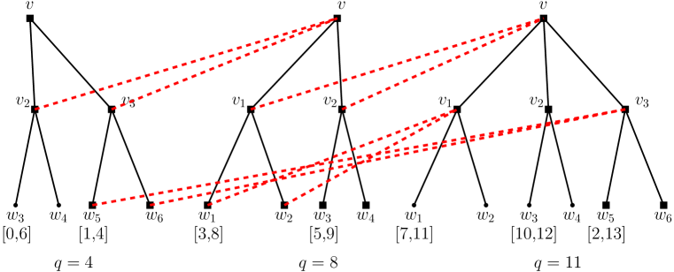
Figure 5: The trees $F_{v,q}$ returned by ${\textsc{BuildTree}}(q)$ for node $v$ at times $q=4,8,11$ are shown in black/solid. For each, the bold squares are nodes that lie in $S$. These are also nodes of the charging forest ${{\cal F}^{ch}}(v)$, whose edges are shown in red/dashed. The request intervals for only the relevant leaf nodes are shown: each bold square is associated with the leaf request below it with the earliest end time. For example, the interval associated with $v_{3}$ at time $q=11$ is $[2,13]$: since this interval is active at time $q=4$, we have edges from $(v_{3},q=11)$ to nodes $(w_{5},q=4),(w_{6},q=4)$ spawned by $v_{3}$ at time $q=4$.

Each node $v$ maintains a charging forest ${{\cal F}^{ch}}(v)$, which we use to build a lower bound on the value of the optimal solution for servicing the outstanding requests below $v$, assuming there is just one available server. The construction here is inspired by the analysis of [AGGP17]. We use this charging forest to add constraints to $\mathfrak{L}^{v}$ (during SimpleUpdate procedure) and to build a corresponding dual solution. We need one more piece of notation: for node $w$ and time $q$, let $\ell$ be the leaf below $w$ such that the active request at $\ell$ has the earliest deadline after $q$. (In case no active request lies below $w$ at time $q$, this is undefined). Let $I$ be the corresponding request interval at $\ell$. We use ${\mathsf{EarliestLeafReq}}(w,q)$ to denote the pair $(\ell,I)$.

The procedure ${\textsc{BuildWitness}}(q,w,v)$ adds a new vertex called $(w,q)$ to the charging forest ${{\cal F}^{ch}}(v)$. To add edges, let $q^{\prime}<q$ be the largest time such that ${{\cal F}^{ch}}(v)$ contains a vertex of the form $(w,q^{\prime})$. Let $(\ell,I)$ denote ${\mathsf{EarliestLeafReq}}(w,q)$. If time $q^{\prime}$ also belongs to $I$, we add in an edge from $(w,q)$ to $(w^{\prime},q^{\prime})$ for every node $w^{\prime}$ that was spawned by $w$ in the call to ${\textsc{BuildTree}}(v,q^{\prime})$. (See Figure 5.)

Here’s the intuition behind this construction: at time $q^{\prime}$, there were outstanding leaf requests below each of the nodes $w^{\prime}$ which were spawned by $w$. The reason that interval $I$ was not serviced at time $q^{\prime}$ (i.e., the leaf $\ell$ was not part of the tree returned by ${\textsc{BuildTree}}(q^{\prime},v)$) was because the intervals chosen in that tree were preferred over $I$, and the total cost of servicing them was already too high. This allows us to infer a lower bound.

6.2 Reminder: Truncated Constraints

We now describe the procedures SimpleUpdate and FullUpdate in detail; both of these procedures will add (truncated) constraints of the form $\varphi_{A,f,\boldsymbol{\tau},v}$ to the local LP for a node $v$ as defined in (5). For sake of completeness, we formally define this notion here:

Definition 6.1 (Truncated Constraints).

Consider a node $v$, a subset $A$ of nodes in $T_{v}$ (where no two them have an ancestor-descendant relationship), a function $f:A\to\mathfrak{R}$ mapping each node $u\in A$ to a request $(\ell_{u},[b_{u},e_{u}])$ at some leaf $\ell_{u}$ below $u$, and an assignment $\tau_{u}$ of timesteps to each $u\in T^{A}_{v}$. The timesteps $\boldsymbol{\tau}$ must satisfy the following two (monotonicity) properties: (a) For each node $u\in T^{A}_{v}$, $\tau_{u}\geq\max_{w\in A\cap T_{u}}e_{w}$; (b) If $v_{1},v_{2}$ are two nodes in $T^{A}_{v}$ with $v_{1}$ being the ancestor of $v_{2}$, then $\tau_{v_{1}}\geq\tau_{v_{2}}.$ Given such a tuple $(A,f,\boldsymbol{\tau},v)$, the truncated constraint $\varphi_{A,f,\boldsymbol{\tau},v}$ (ending at timestep $\tau_{v}$) is defined as follows:

$$\sum_{u\in A\cap T_{v},u\neq v}y^{v}(u,(b_{u},\tau_{p(u)}])+\sum_{u\in T^{A}_{v}\setminus A,u\neq v}y^{v}(u,(\tau_{u},\tau_{p(u)}])\geq|A\cap T_{v}|-k_{v,\tau_{v}}-2\delta(n-n_{v}).$$

6.3 The Simple Update Procedure

The SimpleUpdate procedure is called with parameters: node $v_{i}$, timestep $\tau$ with $\lfloor\tau\rfloor=q$, and target dual increase $\xi$. In the case without time-windows, this procedure merely added a single $\bot$-constraint. Since we may now satisfy requests due to piggybacking, the new version of SimpleUpdate adds other constraints and raises the dual variables corresponding to them.

Recall that BuildTree defines an estimate ${\textsf{cost}}(q)$ and sets ${\textsf{logcost}}(q)=\lfloor\log_{\lambda}2\lambda{\textsf{cost}}(q)\rfloor$. After defining $\Gamma(v_{i},\tau):=\xi$, SimpleUpdate tries to add a constraint to $\mathfrak{L}^{v_{i}}$—for this purpose we use the highest index ${i^{\star}}\leq i$ for which we have previously added a node to the charging forest ${{\cal F}^{ch}}(v_{i^{\star}})$ at time $q$. Hence we set ${i^{\star}}:=\min(i,{\textsf{logcost}}(q))$. As explained in §6.1.1, ${{\cal F}^{ch}}(v_{i^{\star}})$ has a tree rooted at $(v_{i^{\star}},q)$, call it ${\mathcal{T}}$. The algorithm now splits in two cases:

1. Tree ${\mathcal{T}}$ is just the singleton vertex $(v_{i^{\star}},q)$: we add a $\bot$-constraint in line (8) and add $\tau$ to $\mathcal{R}^{s}(v_{i})$. The intuition is that the tree ${\mathcal{T}}$ gives us a lower bound for serving the piggybacked requests. So if it has no edges, we cannot add a non-$\bot$ constraint.

2. Tree ${\mathcal{T}}$ has more than one vertex: in this case we add a (non-$\bot$) constraint to $\mathfrak{L}^{v_{i}}$, details of which are described below.

0.1$\Gamma(v_{i},\tau)\leftarrow\xi$, add $\tau$ to ${\sf Awake}(v_{i})$. ;

0.2 $i^{\star}\leftarrow\min(i,{\textsf{logcost}}(q))$. ;

0.3 if the charging tree ${\mathcal{T}}$ in ${{\cal F}^{ch}}(v_{i^{\star}})$ containing $(v_{i^{\star}},q)$ is a singleton then

0.4       ${\mathfrak{L}}^{v_{i}}(\tau)\leftarrow$ $\bot$-constraint for $\varphi_{A,f,\boldsymbol{\tau},v_{i}}$, where $A=\{v_{i}\},f(v_{i})=(\textsf{ReqLoc}(\tau),\operatorname{\textsf{ReqInt}}(\tau)),\tau_{v_{i}}=\tau$; add $\tau$ to $\mathcal{R}^{s}(v_{i})$ // solitary timestep for $v_{i}$

0.5else

0.6       Let $s$ be such that level-$s$ leaves $\mathcal{L}_{s}$ in ${\mathcal{T}}$ have cost at least $c_{v_{i^{\star}}}/H$. // ${\mathcal{T}}$ not a singleton ;

0.7       foreach $a_{j}=(u_{j},q_{j})\in\mathcal{L}_{s}$ do

0.8             Let $(\ell_{j},R_{j}=[b_{j},e_{j}])$ be ${\mathsf{EarliestLeafReq}}(a_{j})$ as defined in line (7) of ${\textsc{BuildWitness}}(q_{j},u_{j},v_{i^{\star}})$. ;

0.9             add $u_{j}$ to $A$, define $\tau_{u_{j}}\leftarrow b_{i}$, $f(u_{j})=(\ell_{j},R_{j})$. ;

0.10            

0.11      define $\tau_{w}\leftarrow\tau$ for each internal node $w$ in $T^{A}_{v_{i}}$. ;

0.12       add the constraint $\varphi_{A,f,\boldsymbol{\tau},v_{i}}$ (as shown in (21)) to ${\mathfrak{L}}^{v_{i}}(\tau)$, and set the dual variable accordingly; add $\tau$ to $\mathcal{R}^{ns}(v_{i})$ // non-solitary timestep for $v_{i}$

Algorithm 8 $\textsc{SimpleUpdate}(v_{i},\tau,\xi)$

It remains to describe how to add the local constraints and set the dual variables in case ${\mathcal{T}}$ contains more than one node. Recall that ${\mathcal{T}}$ is rooted at $(v_{i^{\star}},q)$. The BuildTree procedure ensures that the nodes spawned by any node $w$ cost at least $c_{w}$; applying this inductively ensures that if $\mathcal{L}$ is the set of leaves of this tree ${\mathcal{T}}$, we have $\sum_{a\in\mathcal{L}}c_{a}\geq c_{v_{i^{\star}}}$. (Here we abuse notation by defining the cost of a tuple $a=(w,q)$ in ${\mathcal{T}}$ to equal the cost of the node $w$.) Hence, there is some level $j$ such that leaves in ${\mathcal{T}}$ corresponding to level-$j$ nodes have cost at least $\nicefrac{{c_{v_{i^{\star}}}}}{{H}}$. Let these leaves of ${\mathcal{T}}$ be denoted $\mathcal{L}_{s}:=\{a_{j}=(u_{j},q_{j})\}_{j=1}^{r}$.

For each leaf $a_{j}=(u_{j},q_{j})\in\mathcal{L}_{s}$ of this charging tree, let $(\ell_{j},R_{j}=[b_{j},e_{j}])$ denote ${\mathsf{EarliestLeafReq}}(a_{j})$ (as in line (7) of ${\textsc{BuildWitness}}(q_{j},u_{j},v_{i})$). Define $A:=\{u_{j}\mid\exists q_{j}\text{ s.t. }(u_{j},q_{j})\in\mathcal{L}_{j}\}$ to be the subset of nodes of the original tree $T$ corresponding to the nodes $\mathcal{L}_{s}$ from the charging tree, and define $f:u_{j}\mapsto(\ell_{j},R_{j})$. Recall that $T^{A}_{v_{i}}$ denotes the minimal subtree rooted at $v_{i}$ and containing $A$ (as leaves). For each node $u_{j}\in A$, define $\tau_{u_{j}}=b_{j}$. Define the timestep $\tau_{w}$ for each internal node $w$ in $T^{A}_{v_{i}}$ to be $\tau$. (Note that ${\mathcal{T}}$ was rooted at $v_{i^{\star}}$, but we define $\tau$ for the portion of the backbone from $v_{i^{\star}}$ up to $v_{i}$ as well.) We will show in Corollary 7.14 that setting $\tau_{v_{i^{\star}}}$ to $\tau$ does not violate the monotonicity property, i.e., $e_{j}\leq q\leq\tau$ for all request intervals $R_{j}$.

Now we add to ${\mathfrak{L}}^{v_{i}}(\tau)$ the truncated constraint $\psi_{A,f,\boldsymbol{\tau},v_{i}}$, which can be written succinctly as

$$\sum_{u_{j}\in A}y^{v_{i}}(u_{j},(b_{j},\tau])\geq|A|-k_{v_{i},\tau_{v_{i}}}-2\delta(n-n_{v_{i}}),$$ (21)

Observe that the RHS above is positive because $|A|\geq 1$ and $k_{v_{i},\tau_{v_{i}}}<1-\delta^{\prime}$. Finally, we set the dual variable for this single constraint to $\xi/(|A|-k_{v_{i},\tau_{v_{i}}}-2\delta(n-n_{v_{i}}))$, so that the dual objective increases by exactly $\xi$. We end by declaring timestep $\tau$ non-solitary, and hence adding it to $\mathcal{R}^{ns}(v_{i})$.

6.4 The Full Update Procedure

The final piece is procedure $\textsc{FullUpdate}(v,\tau,\gamma$). This is essentially the version in §4.3, with one change. Previously, if ${\sf activesib}(u_{0},\tau)$ was not empty, we could have had very little server movement, in case most of the dual increase was because of $b^{C_{u_{0}}}$. To avoid this, we now force a non-trivial amount of server movement. When the dual growth reaches $\gamma$, we stop the dual growth, but if there has been very little server movement, we transfer servers from active leaves below ${\sf activesib}(u_{0},\tau)$ in line (9).

The intuition for this step is as follows: in the $\textsc{SimpleUpdate}(v_{i},v_{0},\xi)$ procedure for $v_{i}$ below $v$, we need to match the dual increase (given by $\xi$) by the amount of server that actually moves into $v_{i}$. This matching is based on the assumption that at least $\gamma/\lambda^{h}$ transfer happens during the FullUpdate procedure. By adding this extra step to FullUpdate, we ensure that a roughly comparable amount of transfer always happens.

Finally, let us elaborate on the constraint $C(v,\sigma,\tau)$. This is written as in (9), using the modified composition rule for $k$-ServerTW from Lemma 3.5. Since we did not spell out the details, let us do so now. As before, $u_{0}$ is the principal child of $v$ at $\tau$, and $U:=\{u_{0}\}\cup{\sf activesib}(u_{0},\tau)$. Each of the constraints $C_{u}\in\mathfrak{L}^{u}(\tau_{u}),u\in U$ has the form $\varphi_{A(u),f(u),\boldsymbol{\tau}(u),u}$ for some tuple $(A(u),f(u),\boldsymbol{\tau}(u))$ for node $u$ ending at $\tau_{u}:=\tau(u)_{u}$. Partition the set $U$ into two sets based on whether ${\mathfrak{L}}^{u}(\tau_{u})$ is a $\{\bot\}$-constraint (i.e., whether $\tau$ is in $\mathcal{R}^{s}(u)$ or in $\mathcal{R}^{ns}(u)$): $U^{\prime}:=\{u\in U:C_{u}\text{ is a $\bot$-constraint}\}$, and $U^{\prime\prime}:=U\setminus U^{\prime}$. Recall that $I_{u}$ denotes the interval $(\tau_{u},\tau]$. For a node $u\in U^{\prime}$, the $\bot$ constraint is given by $\varphi_{A(u),f(u),\boldsymbol{\tau}(u),u}$, where $A(u)=\{u\}$, and let $b_{u}$ is the starting time of the request interval corresponding to $f(u)$. Let $I_{u}^{\prime}$ denote the interval $(b_{u},\tau_{u}]$. The new constraint $C(v,\sigma,\tau)$ is the composition $\varphi_{A,f,\boldsymbol{\tau},v}$ of these constraints, and by Lemma 3.5 implies:

$$\underbrace{\sum_{u\in U^{\prime}}y^{v}(u,I_{u}^{\prime})+\sum_{u\in U}\left(y^{v}(u,I_{u})+a^{C_{u}}\cdot y^{v}\right)}_{a^{C(v,\sigma,\tau)}\cdot y^{v}}\geq\underbrace{\sum_{u\in U}\left(D(u,I_{u})+b^{C_{u}}\right)+(n_{v}-\sum_{u\in U}n_{u})\delta}_{\leq b^{C(v,\sigma,\tau)}}.$$ (22)

Observe that the dual update process itself in FullUpdate remains unchanged despite these new added variables corresponding to $I_{u}^{\prime}$: these variables $\{y^{v}(u,\tau)\}_{\tau\in I_{u}^{\prime},u\in U^{\prime}}$ do not appear in line (9). Hence all the steps here exactly match those for the $k$-Server setting, except for line (9). This completes the description of the local updates, and hence of the algorithm for $k$-ServerTW.

0.1 let $h\leftarrow{\textsf{level}}(v)-1$ and $u_{0}\in\chi_{v}$ be child containing the current request $v_{0}:=\textsf{ReqLoc}(\tau)$. ;

0.2 let $U\leftarrow\{u_{0}\}\cup{\sf activesib}(u_{0},\tau)$; say $U=\{u_{0},u_{1},\ldots,u_{\ell}\}$, $L_{U}\leftarrow$ active leaves below $U\setminus\{u_{0}\}$. ;

0.3 add timestep $\tau$ to the event set $\mathcal{R}^{ns}(v)$ and to ${\sf Awake}(v)$. // “non-solitary” timestep for $v$;

0.4 set timer $s\leftarrow 0$, $\Gamma(v,\tau)\leftarrow\gamma$. ;

0.5 repeat

0.6       for $u\in U$ do

0.7             let $\tau_{u}\leftarrow{\sf prev}(u,\tau)$ and $I_{u}=(\tau_{u},\tau]$. ;

0.8             let $C_{u}$ be a slack constraint in ${\mathfrak{L}}^{u}(\tau_{u})$. // slack constraint exists since ${\sf prev}(u,\tau)$ is awake

0.9      let $\sigma\leftarrow(C_{u_{0}},C_{u_{1}},\ldots,C_{u_{\ell}})$ be the resulting tuple of constraints. ;

0.10       add new constraint $C(v,\sigma,\tau)$ to the constraint set ${\mathfrak{L}}^{v}(\tau)$.;

0.11      

0.12      while all constraints $C_{u_{j}}$ in $\sigma$ are slack and dual objective for ${\mathfrak{L}}^{v}(\tau)$ less than $\gamma$ do

0.13             increase timer $s$ at uniform rate. ;

0.14             increase $z_{C(v,\sigma,\tau)}$ at the same rate as $s$. ;

0.15             for all $u\in U$, define $S_{u}:=I_{u}\cap\left(\mathcal{R}^{ns}(u)\cup\{\tau_{u}+\eta\}\right).$ ;

0.16             increase $y^{v}(u,t)$ for $u\in U,t\in S_{u}$ according to $\frac{dy^{v}(u,t)}{ds}=\frac{y^{v}(u,t)}{\lambda^{h}}+\frac{\gamma}{Mn\cdot\lambda^{h}}$. ;

0.17             transfer server mass from $T_{u}$ into $v_{0}$ at rate $\frac{dy^{v}(u,I_{u})}{ds}+\frac{b^{C_{u}}}{\lambda^{h}}$ using the leaves in $L_{U}\cap T_{u}$, for each $u\in U\setminus\{u_{0}\}$ ;

0.18            

0.19      foreach constraint $C_{u_{j}}$ that is depleted do

0.20             if all the constraints in ${\mathfrak{L}}^{u_{j}}(\tau_{u_{j}})$ are depleted then remove $\tau_{u_{j}}$ from ${\sf Awake}(u_{j})$. ;

0.21            

0.22      

0.23until the dual objective corresponding to constraints in ${\mathfrak{L}}^{v}(\tau)$ becomes $\gamma$.;

0.24let $\alpha\leftarrow$ total amount of servers transferred to $v_{0}$ during this function call. ;

0.25 if ${\sf activesib}(u_{0},\tau)\neq\varnothing$ and $\alpha<\frac{\gamma}{4H\lambda^{h}}$ then

0.26       transfer more servers from $L_{U}$ to $v_{0}$ until total transfer equals $\frac{\gamma}{4H\lambda^{h}}$.

Algorithm 9 $\textsc{FullUpdate}(v,\tau$)

7 Analysis for $k$-ServerTW

The analysis for $k$-ServerTW closely mirrors that for $k$-Server; the principal difference is due to the additional intervals $I_{u}^{\prime}$ on the LHS of (22). If the intervals $I_{u}^{\prime}$ are very long, we may get only a tiny lower bound for the objective value of the LPs: raising only a few $y^{v}$ variables variables could satisfy all such constraints. The crucial argument is that the intervals $I_{u}^{\prime}$ are disjoint for any given vertex $v$ and descendant $u^{\prime}$: this gives us approximate dual-feasibility even with these $I_{u}^{\prime}$ intervals, and even with the dual increases performed in the SimpleUpdate procedure. To show this disjointness, we have to use the properties of the charging forest. A final comment: timesteps in $\mathcal{R}^{ns}(v)$ are now added by both FullUpdate and SimpleUpdate, whereas only SimpleUpdate adds timesteps to $\mathcal{R}^{s}(v)$.

7.1 Some Preliminary Facts

Claim 7.1 (Facts about $\Gamma$).

Fix a node $u$ with parent $v$, and timestep $\tau\in\mathcal{R}^{ns}(u)$.

• $\frac{\gamma}{\lambda^{H}}\leq\Gamma(u,\tau)\leq\gamma$.

• If $\textsc{FullUpdate}(v,\tau)$ is called, then $\Gamma(u,\tau)=\gamma$.

• If $\tau$ gets added to $\mathcal{R}^{ns}(u)$ by SimpleUpdate procedure, then the dual objective value for the sole constraint in ${\mathfrak{L}}^{u}(\tau)$ is $\Gamma(u,\tau)$.

Proof.

The first claim follows from the fact that $\Gamma(u,\tau)$ is either set to $\gamma$ (in FullUpdate) or $\lambda^{i}\frac{\gamma}{\lambda^{i_{0}}}$ (in SimpleUpdate), and that $1\leq i\leq i_{0}\leq H$ in line (4). For the second claim, if $\tau$ gets added to $\mathcal{R}^{ns}(u)$ by FullUpdate, then the statement follows immediately. Otherwise it must be the case that $u=v_{i_{0}}$, and we call $\textsc{SimpleUpdate}(u,\tau,\gamma)$ in line (4) of  Algorithm 4, giving $\Gamma(u,\tau)=\gamma$ again.

For the final claim, observe that ${\mathfrak{L}}^{u}(\tau)$ contains a single constraint $C$ given by (21), and we set $z(C)$ to be $\frac{\Gamma(u,\tau)}{|A|-k_{u,q_{u}}-2\delta(n-n_{u})}$. ∎

Claim 7.2 (Facts about $Z_{q}$).

Suppose the leaf $\ell_{q}$ becomes critical at time $q$, and $v_{i}$ is an ancestor of $\ell_{q}$ such that all leaves in $T_{v_{i}}$ (including $\ell_{q}$) are inactive at time $q$. Then $v_{i+1}$ gets added to the set $Z_{q}$.

Proof.

We claim that ${\textsf{logcost}}(q)$ is at least $i+1$. Since there are no active leaves in $T_{v_{i}}$, all the server mass needs to be brought into $\ell_{q}$ from leaves which are outside $T_{v_{i}}$, and so the total cost of this transfer is at least $(1-\delta^{\prime}-\delta)c_{v_{i}}=(1-\delta^{\prime}-\delta)\lambda^{i}$. It follows that ${\textsf{logcost}}(q)=\lfloor\log_{\lambda}(2\lambda\,{\textsf{cost}}(q))\rfloor\geq i+1$. ∎

7.2 Congestion of Intervals for $\bot$-constraints

Recall from line (8) that ${\mathfrak{L}}^{v}(\tau)$ is a $\bot$-constraint (i.e., timestep $\tau\in\mathcal{R}^{s}(v)$) exactly when the component ${\mathcal{T}}$ of the charging forest ${{\cal F}^{ch}}(v_{i^{\star}})$ containing the vertex $(v_{i^{\star}},\lfloor\tau\rfloor)$ is a singleton.

Lemma 7.3 (Low Congestion I).

For a vertex $v$, let $Q$ be a set of times such that for each $q\in Q,$ there exists a timestep $\tau_{q}\in\mathcal{R}^{s}(v)$ satisfying $\lfloor\tau_{q}\rfloor=q$. Let $\ell_{q}:=\textsf{ReqLoc}(q)$ and $[b_{q},q]=\operatorname{\textsf{ReqInt}}(q)$ be the request location and interval corresponding to time $q$. Then the set of intervals $\{[b_{q},q]\}_{q\in Q}$ has congestion at most $H$.

Proof.

For brevity, let $J_{q}:=[b_{q},q]$; $i^{\star}_{q}$ be the value of ${i^{\star}}$ used in the call to SimpleUpdate on $v$ at timestep $\tau_{q}$ that added the $\bot$-constraint.

Claim 7.4.

Suppose there are times $p<q\in Q$ such that $p\in J_{q}$. Then $i^{\star}_{p}<i^{\star}_{q}$.

Proof.

Let $v_{\operatorname{lca}}$ be the least common ancestor of leaves $\ell_{p}$ and $\ell_{q}$, and $v_{m}$ be the higher of $v_{\operatorname{lca}}$ and $v_{i^{\star}_{p}}$. We first give two useful subclaims.

Subclaim 7.5.

Let $v_{i}$ be an ancestor of $\ell_{q}$. Suppose $v_{i}$ gets added to the set $Z_{q^{\prime}}$ for some $q^{\prime}\in[p,q)$. Then the set $S$ returned by ${\textsc{FindLeaves}}(q^{\prime},v_{i})$ is non-empty.

Proof.

Since (a) the request at $\ell_{q}$ starts before $p$ (and hence before $q^{\prime}$), (b) the node $\ell_{q}\in T_{v_{i}}$, and (c) the request at $\ell_{q}$ is not serviced until time $q$ and hence is still active at time $q^{\prime}$, the set $S$ cannot be empty. ∎

Subclaim 7.6.

If $i^{\star}_{q}<m$, then there exists a $q^{\prime}\in[p,q)$ such that $v_{i^{\star}_{q}}\in Z_{q^{\prime}}$.

Proof.

Figure 6: Illustration of proof of Subclaim 7.6: we consider the interesting case when $v_{m}=v_{i^{\star}_{p}}.$

First consider the case when $i^{\star}_{q}<\operatorname{lca}$. At time $p$, the fact that $\tau_{p}\in{\mathcal{R}^{s}}(v)$ implies that no leaf in $T_{v}$ other than $\ell_{p}$ is active (i.e., has more than $\delta$ amount of server mass). Therefore, at time $p$, no leaf below $v_{i^{\star}_{q}}$ is active. We claim that there must have been a time $q^{\prime}\in(p,q)$ at which a request below $v_{i^{\star}_{q}}$ became critical. Indeed, if not, all leaves below $v_{i^{\star}_{q}}$ continue to remain inactive until time $q$. But then ${\textsf{cost}}(q)\geq(1-\delta^{\prime}-\delta)\lambda^{i^{\star}_{q}}$, and so ${\textsf{logcost}}(q)>i^{\star}_{q}$, a contradiction. So let $q^{\prime}$ be the first time in $(p,q)$ when a request below $v_{i^{\star}_{q}}$ became critical. Repeating the same argument shows that $i^{\star}_{q^{\prime}}\geq i^{\star}_{q}$, and so $v_{i^{\star}_{q}}$ would be added to $Z_{q^{\prime}}$.

The other case is when $\operatorname{lca}\leq i^{\star}_{q}<m$, which means that $m>\operatorname{lca}$ and so $m=i^{\star}_{p}$. In that case $v_{i^{\star}_{q}}$ is added to the set $Z_{p}$ itself. ∎

Now if $i^{\star}_{q}<m$, then Subclaim 7.6 says that $v_{i^{\star}_{q}}$ is added to some $Z_{q^{\prime}}$ for $q^{\prime}\in[p,q)$. By Subclaim 7.5 the set returned by ${\textsc{FindLeaves}}(q^{\prime},v_{i^{\star}_{q}})$ is non-empty: this means $(v_{i^{\star}_{q}},q)$ cannot be a singleton component. This would contradict the fact that $\tau_{q}\in\mathcal{R}^{s}(v)$. Similarly, if $i^{\star}_{q}=m=i^{\star}_{p}$, then $v_{i^{\star}_{p}}=v_{i^{\star}_{q}}$ and the argument immediately above also holds for $q^{\prime}=p$. Hence, it must be that $i^{\star}_{q}>i^{\star}_{p}$, which proves Claim 7.4. ∎

Claim 7.4 implies that $p$ belongs to at most $H$ other intervals $\{J_{q}\}_{q\in Q}$. Indeed, if $p$ lies in the intervals for $q<q^{\prime}<\cdots$, then $q$ also lies in the interval for $q^{\prime}$, etc. Hence the ${i^{\star}}$ values for $p,q,q^{\prime},q^{\prime\prime},\ldots$ must strictly increase, but then there can be only $H$ of them, proving Lemma 7.3. ∎

7.3 Relating the Dual Updates to ${i^{\star}}$

We first prove a bound on the number of iterations of the while loop in Algorithm 4: this uses the lower bound on the server transfer that is ensured by line (9)).

Claim 7.7.

Suppose a request at $v_{0}$ becomes critical at time $q$. The total number of iterations of while loop in Algorithm 4 is at most $\frac{8H{\textsf{cost}}(q)}{\gamma}$.

Proof.

Let the ancestors of $v_{0}$ be labeled $v_{0},v_{1},\ldots,v_{H}$. If the cheapest way of moving the required mass of servers to $v_{0}$ at time $q$ moves $\alpha_{i}$ mass from the active leaves which are descendants of siblings of $v_{i}$, then ${\textsf{cost}}(q)=\sum_{i}\alpha_{i}c_{v_{i}}$.

For an ancestor $v_{i}$ of $v_{0}$, define $t_{i}$ to be the earliest timestep by which either the algorithm moves at least $\alpha_{i}$ server mass from active leaves below the siblings of $v_{i}$ to $v_{0}$, or ${\sf activesib}(v_{i},t_{i})$ becomes empty. Since we transfer at least $\nicefrac{{\gamma}}{{4Hc_{v_{i}}}}$ amount of server mass from leaves below the siblings of $v_{i}$ to $v_{0}$ during each timestep in $(q,t_{i}]$, the number of timesteps in $(q,t_{i}]$ cannot exceed $\nicefrac{{4Hc_{v_{i}}\alpha_{i}}}{{\gamma}}$.

During the algorithm, the set of active siblings of a node $v_{i}$ may become empty at $t_{i}$ while leaving up to $\delta$ amount of server mass at a some leaves below the siblings of $v_{i}$. While calculating ${\textsf{cost}}(q)$, we had allowed leaving only $\delta-\gamma$ amount of server at a leaf, and so it is possible that the algorithm may move an additional $\gamma n$ amount of server mass beyond what has been transferred by $\max_{i}t_{i}$. Since we move at least $\frac{\gamma}{4H\Delta}$ amount of server in each call to FullUpdate procedure, it follows the total number of such calls (beyond $\max_{i}t_{i}$) would be at most $4H\Delta n.$ Therefore, the total number of timesteps before we satisfy the request at $v_{0}$ is at most

$$4H\Delta n+\max_{i}\frac{4Hc_{v_{i}}\alpha_{i}}{\gamma}\leq\frac{4H\delta^{\prime}}{\gamma}+\sum_{i}\frac{4Hc_{v_{i}}\alpha_{i}}{\gamma}=\frac{8H{\textsf{cost}}(q)}{\gamma},$$

where we have used the fact that ${\textsf{cost}}(q)\geq\delta^{\prime}\geq\gamma n\Delta$. ∎

Next, we relate ${i^{\star}}$ from the SimpleUpdate procedure to the increase in the dual variables.

Lemma 7.8.

Suppose a request at $v_{0}$ becomes critical at time $q$. Let $v_{0},v_{1},\ldots,v_{H}$ be the path to the root. For indices $i^{\prime}\leq i$, let $S(i,i^{\prime})$ be the set of timesteps $\tau$ such that (a) $\lfloor\tau\rfloor=q$, and (b) we call $\textsc{SimpleUpdate}(v_{i},\tau,\xi_{\tau})$ for some value of $\xi_{\tau}$, and (c) $i^{\star}=i^{\prime}$ during this function call. Then

$$\sum_{\tau\in S(i,i^{\prime})}\xi_{\tau}\leq 12Hc_{v_{i^{\prime}}}.$$

Proof.

Suppose that $i^{\prime}={i^{\star}}<i$, then $i^{\prime}={\textsf{logcost}}(q)$ for all timesteps $\tau\in S(i,i^{\prime})$. Since the parameter $\xi_{\tau}\leq\gamma$ for any timestep $\tau\in S(i,i^{\prime})$ by 7.1(i), Claim 7.7 implies that $\sum_{\tau\in S(i,i^{\prime})}\xi_{\tau}\leq|S(i,i^{\prime})|\;\gamma\leq 8H{\textsf{cost}}(q).$ But ${\textsf{cost}}(q)\leq\lambda^{{\textsf{logcost}}(q)}=\lambda^{i^{\prime}}=c_{v_{i^{\prime}}}$, which completes the proof of this case.

The other case is when $i^{\prime}=i$. We claim that for any timestep $\tau\in S(i,i^{\prime})$, at least $\frac{\xi_{\tau}}{4Hc_{v_{i}}}$ amount of server reaches the requested node. Indeed, we know that $i_{0}\geq i$ at this timestep, so line (9) of the FullUpdate procedure ensures that at least $\frac{\gamma}{4H\lambda^{i_{0}}}=\frac{\xi_{\tau}}{4Hc_{v_{i}}}$ amount of server reaches $v_{0}$, where we used that $\xi_{\tau}=\lambda^{i_{0}-i}\gamma$. Since at most one unit of server reaches $v_{0}$ when summed over all timesteps corresponding to $q$, we get

$$\sum_{\tau\in S(i,i^{\prime})}\xi_{\tau}\leq 4Hc_{v_{i}}.\qed$$

7.4 Proving the Invariant Conditions

We begin by stating the invariant conditions and show that these are satisfied. Invariant (I2) statement only changes slightly: we replace $\gamma$ by $\Gamma(v,\tau)$ as given below.

Invariant (I5).

At the end of each timestep $\tau\in\mathcal{R}^{ns}(v)$, the objective function value of the dual variables corresponding to constraints in ${\mathfrak{L}}^{v}(\tau)$ equals $\Gamma(v,\tau)$. I.e., if a generic constraint $C$ is given by $\langle a^{C}\cdot y^{v}\rangle\geq b^{C}$, then

$$\sum_{C\in{\mathfrak{L}}^{v}(\tau)}b^{C}\cdot z_{C}=\Gamma(v,\tau)\qquad\forall\tau\in\mathcal{R}^{ns}(v).$$ (I5)

Furthermore, $b^{C}>0$ for all $C\in\mathfrak{L}^{v}(\tau)$ and $\tau\in\mathcal{R}(v)$.

(iii) shows that the invariant above is satisfied whenever $\tau$ gets added to $\mathcal{R}^{ns}(v)$ by SimpleUpdate, and the second statement follows from the comment after (21). As before, the quantity ${\sf loss}(u,\tau)$ is defined by (10) whenever $\textsc{FullUpdate}(v,\tau)$ is called, $v$ being the parent of $u$. The invariant condition (I4) is replaced by the following which also accounts for the extra transfer which happens during line (9) in $\textsc{FullUpdate}(v,\tau)$ procedure:

Invariant (I6).

Consider a node $v$ and timestep $\tau$ such that $\textsc{FullUpdate}(v,\tau)$ is called. Let $u$ be the $v$’s principal child at timestep $\tau$. The server mass entering subtree $T_{u}$ during the procedure $\textsc{FullUpdate}(v,\tau)$ is at most

$$\frac{\gamma-{\sf loss}(u,\tau)}{\lambda^{h}}+\frac{\gamma}{4H\lambda^{h}}.$$ (I6)

We again use the ordering $\prec$ on pairs $(v,\tau)$ and assume that the above two invariant conditions holds for all $(v,\tau)\prec({v^{\star}},{\tau^{\star}})$. We now outline the main changes needed in the analysis done in Section 5.1.  Claim 5.5 still holds with the same proof. We can again define ${\sf fill}(u,\tau),\tau\in\mathcal{R}^{ns}(u)$ as in (11). Note that $\tau^{\prime}\in{\sf fill}(u,\tau)$ only if $\textsc{FullUpdate}(v,\tau)$ is called, where $v$ is the parent of $u$. Claim 5.7 still holds with the same proof. The statement of Claim 5.8 changes to the following:

Claim 7.9.

Let $\tau\in\mathcal{R}(u)$ for some $\tau<{\tau^{\star}}$. The server mass entering $T_{u}$ at timestep $\tau$ is at most

$$\left(1+\frac{1}{\lambda-1}\right)\left(1+\frac{1}{4H}\right)\frac{\Gamma(u,\tau)}{\lambda^{{\textsf{level}}(u)}}-\frac{{\sf loss}(u,\tau)}{\lambda^{{\textsf{level}}(u)}}.$$

Proof.

Consider the iteration of the while loop of Algorithm 4 corresponding to timestep $\tau$. First consider the case when $u$ happens to be $v_{i},i\geq i_{0}$. In this case, $\Gamma(u,\tau)=\gamma$. The result follows as in the proof of Claim 5.8, where the extra term of $\frac{\gamma}{4H\lambda^{h}}$ arises because of line (9) in the FullUpdate procedure.

Now consider the case when $u$ is a vertex of the form $v_{i},i<i_{0}$. Note that $\frac{\gamma}{\lambda^{h_{0}}}=\frac{\Gamma(v_{i},\tau)}{\lambda^{h}}$, and so the result follows in this case as well by using Invariant (I6), and the quantity ${\sf loss}(u,\tau)=0$ here. ∎

The classification of $g(w,\tau)$ into $g^{\mathsf{loc}}(w,\tau),g^{\mathsf{inh}}(w,\tau)$ holds as before. The statement of Lemma 5.9 changes as given below, and the proof follows the same lines. We assume that $\textsc{FullUpdate}({v^{\star}},{\tau^{\star}})$ is called.

Lemma 7.10.

Let $u$ be a non-principal child of ${v^{\star}}$ at timestep ${\tau^{\star}}$, and $I:=(\tau_{1},{\tau^{\star}}]$ for some timestep $\tau_{1}<{\tau^{\star}}$. Let $S$ be the timesteps in $\mathcal{R}^{ns}(u)\cap(\tau_{1},{\tau^{\star}}]$ that have been removed from ${\sf Awake}(u)$ by the moment when $\textsc{FullUpdate}({v^{\star}},{\tau^{\star}})$ is called. Then

$$g^{\mathsf{inh}}(u,(\tau_{1},{\tau^{\star}}])\geq\left(1+\frac{1}{2H}\right)\,\frac{\Gamma(u,S)}{\lambda^{{\textsf{level}}(u)}}-\sum_{\tau\in S}\frac{{\sf loss}(u,\tau)}{\lambda^{{\textsf{level}}(u)}},$$

where $\Gamma(u,S)=\sum_{\tau\in S}\Gamma(u,\tau)$.

The statement and proof of Corollary 5.10 remains unchanged. The proof of Claim 5.11 also remains unchanged, though we now need to use (i) (part (iii)). We now restate the analogue of Claim 5.12:

Claim 7.11 (Inductive Step Part I).

Consider the call $\textsc{FullUpdate}({v^{\star}},{\tau^{\star}})$, and let $u_{0}$ be the principal child of ${v^{\star}}$ at this timestep. Suppose ${\sf activesib}(u_{0},{\tau^{\star}})\neq\varnothing$. Then the dual objective value corresponding to the constraints in ${\mathfrak{L}}^{v^{\star}}({\tau^{\star}})$ equals $\gamma$; i.e.,

$$\sum_{C\in{\mathfrak{L}}^{v^{\star}}({\tau^{\star}})}z_{C}\,b^{C}=\gamma.$$

Moreover, the server mass entering $T_{u_{0}}$ going to the request node in this call is at most

$$\frac{\gamma-{\sf loss}(u_{0},{\tau^{\star}})}{\lambda^{h}}+\frac{\gamma}{4H\lambda^{h}}.$$

Since the update rule for the $y^{v}$ variables in line (9) of the FullUpdate procedure does not consider the intervals $I_{u}^{\prime}$ (as stated in (22)), the proof proceeds along the same lines as that of Claim 5.12. The extra additive term of $\frac{\gamma}{4H\lambda^{h}}$ appears due to line (9) in FullUpdate procedure. The statement and proof of Claim 5.14 remain unchanged. This shows that the two invariant conditions (I5) and (I6) are satisfied. Finally, we state the analogue of Corollary 5.15 which bounds the parameter $M$.

Corollary 7.12.

For node $u$ and timestep $\tau$, let $\tau_{u}:={\sf prev}(u,\tau)$. There are at most $\frac{5H\lambda^{2H}k}{2\gamma}$ timesteps in $(\tau_{u},\tau]\cap\mathcal{R}^{ns}(u)$. So we can set $M$ to $\frac{5H\lambda^{2H}k}{2\gamma}+1$.

Proof.

The proof proceeds along the same lines as that of Corollary 5.15, except that the analogue of (13) now becomes:

$$g^{\mathsf{inh}}(u,I)-r(u,I)\geq\left(\frac{1}{2H}-\frac{1}{\lambda-1}\left(1+\frac{1}{4H}\right)\right)\frac{\Gamma(u,S)}{\lambda^{h}}\geq\frac{2}{5H}\cdot\frac{\gamma|S|}{\lambda^{2H}},$$

where the last inequality uses (ii)(i). This implies the desired upper bound on $|S|$. ∎

This shows that the algorithm FullUpdate is well defined. Next we give properties of the charging forest, and then show that the dual variables in each of the local LPs are near-feasible.

7.5 Properties of the Charging Forest

Fix a vertex $v$ and consider the charging forest ${{\cal F}^{ch}}(v)$. Recall the notation from §6.1.1: a node in this forest is a tuple $a_{i}=(w_{i},q_{i})$, and has a corresponding leaf request ${\mathsf{EarliestLeafReq}}(w_{i},q_{i})=(\ell_{i},R_{i}=[b_{i},e_{i}])$. We begin with a monotonicity property, which is useful to show that (21) is properly defined (and the $\boldsymbol{\tau}$ values are “monotone”).

Claim 7.13 (Monotonicity I).

Suppose $a_{2}=(w_{2},q_{2})$ is the parent of $a_{1}=(w_{1},q_{1})$ in the forest ${{\cal F}^{ch}}(v)$. Then, $e_{1}\leq e_{2}$.

Proof.

By definition of an edge in ${{\cal F}^{ch}}(v)$, the request interval $R_{2}$ for $a_{2}$ must contain $q_{1}$. At time $q_{1}$, the function ${\textsc{FindLeaves}}(w_{2},q_{1})$ would have returned $w_{1}$ as one of the vertices in the set $S$ (i.e., $w_{2}$ would have spawned $w_{1}$ at time $q_{1}$), and $R_{2}$ was also an request below $w_{2}$ at time $q_{1}$, so $R_{1}$ must end no later than $R_{2}$ does. ∎

Corollary 7.14 (Monotonicity II).

Let $a_{i}=(w_{i},q_{i})$ belong to a tree ${\mathcal{T}}$ of ${{\cal F}^{ch}}(q)$ rooted at $(v,q)$. Then $q_{i}<e_{i}\leq q$.

Proof.

The first fact uses that $R_{i}$ is active at time $q_{i}$. The second fact follows by repeated application of Claim 7.13, and that the earliest leaf request at the root $(v,q)$ corresponds to the request critical at time $q$, which ends at $q$. ∎

The next result shows another key low-congestion property of the charging forest, which we then use to build lower bounds for any single-server instance.

Lemma 7.15 (Low Congestion II).

Consider $u,v$ such that $u\in T_{v}$. Let ${\mathcal{T}}_{1},\ldots,{\mathcal{T}}_{l}$ be distinct charging trees in the forest ${{\cal F}^{ch}}(v)$, where ${\mathcal{T}}_{j}$ is rooted at $(v,q_{j})$ and contains a leaf vertex $a_{j}=(u,q_{j}^{\prime})$, with the corresponding ${\mathsf{EarliestLeafReq}}(a_{j})$ denoted $(\ell_{j},R_{j}=[b_{j},e_{j}])$. Then (a) the intervals $\{(q_{j}^{\prime},q_{j}]\}_{j\in[l]}$ have congestion at most $H$, and (b) the set of intervals $\{(b_{j},q_{j}^{\prime}]\}_{j\in[l]}$ are mutually disjoint. Therefore, the set of intervals $\{(b_{j},q_{j}]\}_{j\in[l]}$ have congestion at most $H+1$.

Proof.

Consider a timestep $t$, and let $S_{t}\subseteq[l]$ be the set of indices $j$ such that $t\in(q_{j}^{\prime},q_{j}]$. For each $j\in S_{t}$, consider the path $P_{j}$ from $a_{j}=(u,q_{j}^{\prime})$ to the root $(v,q_{j})$ in ${\mathcal{T}}_{j}$. For sake of concreteness, let this path be $(u_{j}^{1},q_{j}^{1})=(u,q_{j}^{\prime}),(u_{j}^{2},q_{j}^{2}),\ldots,(u_{j}^{n_{j}},q_{j}^{n_{j}})=(v,q_{j})$. Since $t\in(q_{j}^{\prime},q_{j}]$, there is an index $i$ such that $t\in(q_{j}^{i-1},q_{j}^{i}]$—call this index $i(j)$.

Subclaim 7.16.

For any two distinct $j,j^{\prime}\in S_{t}$, $u_{j}^{i(j)}\neq u_{{j^{\prime}}}^{i(j^{\prime})}$.

Proof.

Suppose not. For sake of brevity, let $w$ denote $u_{j}^{i(j)}=u_{{j^{\prime}}}^{i(j^{\prime})}$, $i$ denote $i(j)$ and $i^{\prime}$ denote $i(j^{\prime})$. Assume wlog that $q_{j^{\prime}}^{i^{\prime}}<q_{j}^{i}$. So ${\mathcal{T}}_{j}$ and ${\mathcal{T}}_{j^{\prime}}$ have vertices $(w,q_{j}^{i})$ and $(w^{\prime},q_{j^{\prime}}^{i^{\prime}})$ respectively. Now consider the child of $(u_{j}^{i-1},q_{j}^{i-1})$ of $(w,q_{j}^{i})$. The rule for adding edges in ${\mathcal{T}}_{j}$ states that we look at the highest time $q^{\prime}<q_{j}^{i}$ for which there is a vertex $(w,q^{\prime})$ in the charging forest, and so $q_{j}^{i-1}=q^{\prime}$. Also $q^{\prime}\geq q_{j^{\prime}}^{i^{\prime}}$. But then, the intervals $(q_{j}^{i-1},q_{j}^{i}]$ and $(q_{j^{\prime}}^{i^{\prime}-1},q_{j^{\prime}}^{i^{\prime}}]$ are disjoint, which is a contradiction because both of them contain $t$. ∎

Since all these $u_{j}^{i(j)}$ vertices must lie on the path from $u$ to $v$ in $T$, there are only $H$ of them. Since they are distinct by the above claim, the number of intervals containing $t$ is at most $H$, which proves the first statement.

To prove the second statement, assume w.l.o.g. that $\{q_{j}\}_{j\in[l]}$ are arranged in increasing order. It suffices to show that for any $j\in[l]$, $(b_{j},q_{j}^{\prime}]$ and $(b_{j+1},q_{j+1}^{\prime}]$ are disjoint. Suppose not. Since $e_{j+1}\geq q_{j+1}^{\prime}$ (by Corollary 7.14), we have that $R_{j+1}$ contains $q_{j}^{\prime}$. Since $(u,q_{j+1}^{\prime})$ has no children ${\mathcal{T}}_{j+1}$, the construction of the charging forest means ${\textsc{FindLeaves}}(u,q_{j}^{\prime})$ should have returned the set $S=\varnothing$. Now since $v$ is added to the set $Z_{q_{j}^{\prime}}$, all the active requests—in particular $R_{j+1}$— below $u$ at time $q_{j}^{\prime}$ would be serviced at time $q_{j}^{\prime}$ due to line (4)). This contradicts the fact that $R_{j+1}$ is active at time $q_{j+1}^{\prime}>q_{j}^{\prime}$. ∎

7.6 Dual Feasibility of SimpleUpdate

Fix a vertex $v$ and the local LP $\mathfrak{L}^{v}$, which has variables $y^{v}(u,\tau)$ for $u\in T_{v}$ and timesteps $\tau$. First, consider only the constraints in $\mathfrak{L}^{v}$ added by the SimpleUpdate procedure, i.e., using (21).

Theorem 7.17.

For a variable $y^{v}({u^{\star}},{\tau^{\star}})$, let ${S^{\star}}$ be the set of timesteps $\tau$ such that SimpleUpdate is called on $v$, and the (unique) constraint $C_{\tau}$ (of the form (21)) that it adds to $\mathfrak{L}^{v}(\tau)$ contains the variable $y^{v}({u^{\star}},{\tau^{\star}})$ on the LHS. Then:

$$\sum_{\tau\in{S^{\star}}}z(C_{\tau})\leq O(H^{4})\cdot c_{{u^{\star}}}.$$ (23)

Proof.

In the call to SimpleUpdate, we use the charging tree rooted at a vertex $v_{i^{\star}}$, where $v_{i^{\star}}$ lies between $v$ and ${u^{\star}}$. Motivated by this, for a node $v^{\prime}$ on the path between ${u^{\star}}$ and $v$, let ${S^{\star}}(v^{\prime})$ denote the subset of timesteps $\tau$ for which the corresponding vertex $v_{i^{\star}}$ is set to $v^{\prime}$. We show:

Subclaim 7.18.

For any $v^{\prime}$ on the path between ${u^{\star}}$ and $v$,

$$\sum_{\tau\in{S^{\star}}(v^{\prime})}z(C_{\tau})\leq O(H^{3})\cdot c_{{u^{\star}}}.$$

Proof.

Consider a timestep $\tau\in{S^{\star}}(v^{\prime})$. Let ${\mathcal{T}}_{q}$ be the tree in the charging forest ${{\cal F}^{ch}}(v^{\prime})$ containing $(v^{\prime},q)$ for $q=\lfloor\tau\rfloor$. As described when defining (21), let $\mathcal{L}_{s_{\tau}}$ be the leaves of ${\mathcal{T}}_{q}$ corresponding to level $s_{\tau}$. Since the variable involving ${u^{\star}}$ appears in this constraint, we have ${u^{\star}}\in\mathcal{L}_{s_{\tau}}$. Therefore, each leaf in $\mathcal{L}_{s_{\tau}}$ has cost equal to $c_{u^{\star}}$, By the choice of level, the total cost of this set is at least $\frac{c_{v^{\prime}}}{H}$, so

$$|\mathcal{L}_{s_{\tau}}|\geq\frac{c_{v^{\prime}}}{Hc_{{u^{\star}}}}.$$

Moreover, the tree ${\mathcal{T}}_{q}$ was not a singleton so $c_{{u^{\star}}}\leq c_{v^{\prime}}/\lambda$, and since $\lambda\geq 10H$, we get $|\mathcal{L}_{s_{\tau}}|\geq 10$. Recall that we set

$$z(C_{\tau})=\frac{\xi_{\tau}}{|\mathcal{L}_{s_{\tau}}|-k_{v^{\prime},\tau_{v^{\prime}}}-2\delta(n-n_{v^{\prime}})}\leq\frac{2\xi_{\tau}}{|\mathcal{L}_{s_{\tau}}|},$$

where the inequality uses that all leaves below $v$ (except for the requested leaf) have at most $\delta$ servers, and so $k_{v^{\prime},\tau_{v^{\prime}}}+2\delta(n-n_{v^{\prime}})\leq 1+2n\delta\ll|\mathcal{L}_{s_{\tau}}|/2$. Combine the above two facts, for any time $q$,

$$\sum_{\tau:\tau\in{S^{\star}}(v^{\prime}),\lfloor\tau\rfloor=q}z(C_{\tau})\leq\frac{2Hc_{u^{\star}}}{c_{v^{\prime}}}\cdot\sum_{\tau:\tau\in{S^{\star}}(v^{\prime}),\lfloor\tau\rfloor=q}\xi_{\tau}\leq 24H^{2}\;c_{{u^{\star}}},$$ (24)

where the last inequality follows from Lemma 7.8.

We need to sum over different values of $q$, so consider $Q:=\{\lfloor\tau\rfloor\mid\tau\in{S^{\star}}(v^{\prime})\}$. For each value $q_{j}\in Q$, choose $\tau_{j}$ to be one representative timestep in ${S^{\star}}$ (in case there are many). For each $q_{j}\in Q$, there is a vertex of the form $(u^{\star}_{j},q_{j}^{\prime})$ in the tree in ${{\cal F}^{ch}}(v^{\prime})$ rooted at $(v^{\prime},q_{j})$. The constraint $C_{\tau_{j}}$ involves $y^{v}({u^{\star}},(b_{j},\tau_{j}])$, where $b_{j}$ is the left end-point of the leaf request ${\mathsf{EarliestLeafReq}}({u^{\star}},q_{j}^{\prime})$. And ${\tau^{\star}}$ belongs to all of these intervals $(b_{j},\tau_{j}]$. Write $(b_{j},\tau_{j}]$ as $(b_{j},q_{j}]\cup(q_{j},\tau_{j}]$. The intervals $(q_{j},\tau_{j}]$ are mutually disjoint for all $j$, and the intervals $(b_{j},q_{j}]$ have congestion at most $H+1$ by Congestion Lemma II (Lemma 7.15). Therefore the intervals $(b_{j},\tau_{j}]$ have congestion at most $H+2$, and so $|Q|\leq H+2$. Combining this with (24) completes the proof. ∎

Theorem 7.17 follows from the above claim by summing over all $v^{\prime}$ on the path from ${u^{\star}}$ to $v$. ∎

7.7 Dual Feasibility

In this section, we show approximate dual feasibility of the entire solution due to both the SimpleUpdate and FullUpdate procedures. The proof is very similar to the one for $k$-Server (in §5.2) except for two changes: (i) we need to account for the intervals $I_{u}^{\prime}$ as in (22), and (ii) we have defined new sets of constraints in SimpleUpdate procedure, so the result of Theorem 7.17 needs to be combined with the overall dual feasibility result. Observe that the statements of Claim 5.16 and Claim 5.17 hold without any changes. We now prove the analogue of Lemma 5.19. First, a simple observation.

Claim 7.19.

Consider a time $q$ and vertex $v$ such that a critical request at time $q$ lies below $v$. Then the total objective value of dual variables raised during FullUpdate procedure at $v$ is at most $4Hc_{v}/\lambda$.

Proof.

Let the height of $v$ be $h+1$. During each call of FullUpdate at $v$, we raise the dual objective by $\gamma$ units (by Claim 7.11), and transfer at least $\frac{\gamma}{4H\lambda^{h}}=\frac{\gamma\lambda}{4Hc_{v}}$ server mass to the requested leaf node $\ell_{q}$. Since we transfer at most one unit of server mass to $\ell_{q}$, the result follows. ∎

Theorem 7.20 (Dual Feasibility for Time-Windows).

For a node $v$ at height $h+1$, consider the dual variables $z(C)$ for constraints added in $\mathfrak{L}^{v}$ during the FullUpdate and the SimpleUpdate procedure. These dual variables $z_{C}$ are $\beta_{h}$-feasible for the dual program $\mathfrak{D}^{v}$, where $\beta_{h}=\left(1+\nicefrac{{1}}{{H}}\right)^{h}O(H^{4}+H(\ln n+\ln M+\ln(k/\gamma))).$

Proof.

We prove the claim by induction on the height of $v$. For a leaf node, this follows vacuously, since the primal/dual programs are empty. Suppose the claim is true for all nodes of height at most $h$. For a node $v$ at height $h+1>0$ with children $\chi_{v}$, the variables in ${\mathfrak{L}}^{v}$ are of two types: (i) $y^{v}(u,t)$ for some timestep $t$ and child $u\in\chi_{v}$, and (ii) $y^{v}(u^{\prime},t)$ for some timestep $t$ and non-child descendant $u^{\prime}\in T_{v}\setminus\chi_{v}$.

We consider variables of the first type. Fix a child $u$ and a timestep $\tau$, and let ${\cal C}^{F}$ be the set of constraints in $\mathfrak{L}^{v}$ added in FullUpdate subroutine that contain the variable $y^{v}(u,\tau)$ in the LHS. We group ${\cal C}^{F}$ into three classes of constraints (and draw on the notation in (22)):

• The timestep $t$ lies in $I_{u}=(\tau_{u},\tau]$, where $u$ is a non-principal child of $v$ at the timestep $\tau$ at which this constraint is added: call this set of constraints ${\cal C}_{1}(t)$. The argument here is identical to that in the proof of Lemma 5.19, and so we get

  $$\sum_{C\in{\cal C}_{1}}z_{C}\leq O(\ln n+\ln M+\ln(k/\gamma))c_{u}.$$

• The timestep $t$ lies in the interval $I_{u}^{\prime}=(b_{u},\tau_{u}]$, where $u$ is a non-principal child of $v$ at timestep $\tau_{u}$. Denote the set of such constraints by ${\cal C}_{2}=\{C_{1},\ldots,C_{s}\}$. For sake of concreteness, let the interval $I_{u}^{\prime}$ in $C_{j}$ be $I_{j}^{\prime}=(b_{j},\tau_{j}],$ and let $I_{j}$ denote the corresponding $I_{u}$ interval. Observe that $\tau_{j}$ corresponds to a $\bot$-constraint in $\mathcal{L}^{u}$, and so always remains in ${\sf Awake}(u)$. Let $q_{j}$ denote $\lfloor\tau_{j}\rfloor$. Note that any constraint in ${\cal C}_{2}$ must contain one of the variables $y^{v}(u,q_{j}+1),j\in[s]$, and each of these variables belongs to the corresponding $I_{j}$ interval. So if $X$ denotes the set $\{q_{j}:j\in[s]\}$, then

  $$\sum_{C\in{\cal C}_{2}}z(C)\leq\sum_{t^{\prime}\in X}\sum_{C\in{\cal C}_{1}(t^{\prime}+1)}z(C)\leq O(\ln n+\ln M+\ln(k/\gamma))\cdot|X|\cdot c_{u},$$ (25)

  where the last inequality follows from case (i) above. It remains to bound $|X|.$ We know from the Congestion Lemma I (Lemma 7.3) that the intervals $(b_{j},q_{j}],q_{j}\in X,$ have congestion at most $H$. Since the intervals $(q_{j},q_{j}+1],q_{j}\in X,$ are mutually disjoint, it follows that the intervals $(b_{j},q_{j}+1]$ have congestion at most $H+1$. Since all of them contain the timestep $t$, it follows that $|X|\leq H+1$. This shows that

  $$\sum_{C\in{\cal C}_{2}}z(C)\leq O(H(\ln n+\ln M+\ln(k/\gamma)))c_{u}.$$

• The timestep $t$ lies in the interval $I_{u}^{\prime}=(b_{u},\tau]$, where $u^{\prime}$ is the principal child of $u$ at timestep $\tau$: call such constraints ${\cal C}_{3}$. For a time $q$, let ${\cal C}_{3}(q)$ be the subset of constraints in ${\cal C}_{3}$ which were added at timesteps $\tau$ for which $\lfloor\tau\rfloor=q$. Claim 7.19 shows that

  $$\sum_{C\in{\cal C}_{3}(q)}z(C)\leq 4H\frac{c_{v}}{\lambda}=4H\,c_{u}.$$

  Arguing as in case (ii) above, and again using Congestion Lemma I (Lemma 7.3), we see that there are at most $O(H)$ distinct time $q$ such that the set ${\cal C}_{3}(q)$ is non-empty. Therefore,

  $$\sum_{C\in{\cal C}^{F}}z(C)\leq O(H^{2})c_{u}.$$

Let ${\cal C}$ be the set of all constraints containing $y^{v}(u,t)$. Combining the observations above, and using Theorem 7.17 for the constraints in ${\cal C}$ added due to the SimpleUpdate procedure, we see that

$$\sum_{C\in{\cal C}}z(C)\leq\beta_{0}\,c_{u}.$$

It remains to consider the variables $y^{v}(u^{\prime},\tau)$ with $u^{\prime}\in T_{u}$ and $u\in\chi_{v}$. The argument here follows from induction hypothesis, and is identical to the one in the proof of Lemma 5.19. ∎

7.8 The Final Analysis

We can now put the pieces together: this part is also very similar to §5, except for the cost of the piggybacking trees. Recall that $\lambda\geq 10H$.

1. Theorem 7.20 shows that the dual solution for the global LP (which is the same as the $\mathfrak{L}^{\mathbbm{r}}$) is $O(H^{4}+H\log\nicefrac{{Mnk}}{{\gamma}})$-feasible. In each iteration of the while loop in Algorithm 4, we raise the dual objective corresponding to this LP by $\gamma$ units, as Claim 7.11 shows.

2. The total service cost in each call to the FullUpdate procedure is $O(\gamma)$—again by Claim 7.11, the amount of server mass transferred during FullUpdate procedure at vertex $v$ at height $h+1$ is at most $\frac{\gamma}{\lambda^{h}}$, and the cost of moving a unit of server mass below $T_{v}$ is $O(\lambda^{h})$. Therefore, the cost to service the critical request in each iteration is $O(\gamma H)$. Therefore, the service cost for each critical request is $O(H)$ times the dual objective value.

3. Now we consider the service cost for piggybacked requests. The cost of all the trees is dominated by the cost of tree for $v_{{\textsf{logcost}}(q)}$, i.e., at most

   $$O(H^{2}c_{v_{{\textsf{logcost}}(q)}})=O(H^{2}\;\lambda^{{\textsf{logcost}}(q)})\leq O(H^{2}\lambda\;{\textsf{cost}}(q)).$$

   Since ${\textsf{cost}}(q)$ is the least cost to move the required amount of server to the request location, the cost of the trees is at most $O(H^{2}\lambda)$ times the cost incurred in the previous step.

Hence the competitiveness is

$$O(H^{4}+H\log\nicefrac{{Mnk}}{{\gamma}})\cdot O(H)\cdot O(H^{2}\lambda).$$

It follows that our fractional algorithm for the $k$-ServerTW problem is $O(H^{4}\lambda(H^{3}+\log\nicefrac{{Mnk}}{{\gamma}}))$-competitive. This proves Theorem 1.2.

8 Closing Remarks

Our work suggests several interesting directions for future research. Can our LP extend to variants and generalizations of $k$-Server in the literature? One natural candidate is the hard version of the $k$-taxi problem. Another interesting direction is to exploit the fact that our LP easily extends to time-windows. The special case of $k$-ServerTW where $k=1$ is known as online service with delay. While poly-logarithmic competitive ratios are known for this problem (and also follow from our current work), no super-constant lower bound on its competitive ratio bound is known. On the other hand, a sub-logarithmic competitive ratio is not known even for simple metrics like the line. Can our LP (or a variant) bridge this gap?

More immediate technical questions concern the $k$-ServerTW problem itself. For instance, can the competitive ratio of the $k$-ServerTW problem be improved from $\operatorname{poly}\log(n,\Delta)$ to $\operatorname{poly}\log(k)$? Another direction is to extend $k$-ServerTW to general delay penalties. Often, techniques for time-windows extend to general delay functions by reducing the latter to a prize-collecting version of the time-windows problem. Exploring this direction for $k$-ServerTW would be a useful extension of the results presented in this paper.

Acknowledgments

AG was supported in part by NSF awards CCF-1907820, CCF-1955785, and CCF-2006953. DP was supported in part by NSF awards CCF-1750140 (CAREER) and CCF-1955703, and ARO award W911NF2110230.

Appendix A Relating $\mathfrak{M}$ to the Min-cost Flow Formulation for $k$-Server

We show that the constraints (2) of the LP relaxation $\mathfrak{M}$ for $k$-Server are implied by the standard min-cost flow formulation for $k$-Server on HSTs.

We first describe the min-cost flow formulation in detail. Consider an instance of the $k$-Server problem consisting of an HST $T$, and a sequence of $N$ request times. Recall that the set of timesteps ${\mathcal{T}}$ varies from $1$ to $N$ in steps of $\eta$. We construct a time-expanded graph $G$ with vertices $V(G):=\{v_{t}\mid v\in V(T),t\in{\mathcal{T}}\}\cup\{s_{G},t_{G}\}$. The edges are of three types (there are no edge-capacities):

• cost-$0$ edges $\{(s_{G},v_{1}),(v_{N},t_{G})\mid v\in V(T)\}$ connecting the source and sink to the first and last copies of each node,

• cost-$0$ edges $\{(v_{t},v_{t+1})\mid v\in V(T),t\in{\mathcal{T}}\}$ between consecutive copies of the same vertex, and

• edges $\{(v_{t},p(v)_{t})\mid v\in V(T),t\in{\mathcal{T}}\}$ of cost $c_{v}$ between each node and its parent, and $\{(v_{t},u_{t})\mid v\in V(T),u\in\chi_{v},t\in{\mathcal{T}}\}$ of cost zero between a node and its children. (This captures that moving servers up the tree incurs cost, but moving down the tree can be done free of charge.)

The source $s_{G}$ has $k$ units of supply, and sink $t_{G}$ has $k$ units of demand (or equivalently, a supply of $-k$). If the request for time $q$ is at leaf $\ell$, we require that at least one unit of flow passes through $\ell_{q}$. To model this, we assign a supply of $-1$ to $\ell_{q}$ and $+1$ to $\ell_{q+1}$. This is consistent with the proof of Claim 2.1 where we assumed that after servicing $\ell$ at time $q$, the server stays at this leaf till time $q+1$.

The integrality of the min-cost flow polytope implies that an optimal solution to this transportation problem captures the optimal $k$-server solution. Moreover, the max-flow min-cut theorem says that if $x$ is a solution to this transportation problem, then for all subsets $S\subseteq V(G)$,

$$x(\partial^{+}(S))\geq{\mathsf{supply}}(S).$$ (26)

We now consider special cases of these constraints. Consider a tuple $(A,\boldsymbol{\tau})$ corresponding to the LP constraint (2): recall that $A$ is a subset of leaves, and $\boldsymbol{\tau}$ assigns a timestep $\tau_{u}$ to each $u\in T^{A}$, with these timesteps satisfying the “monotonicity” constraints stated before (2). We now define a set $S_{A,\boldsymbol{\tau}}$ as follows: for each node $v\in T^{A}$, we add the nodes $v_{t},t>\tau_{v}$ to $S_{A,\boldsymbol{\tau}}$. Finally, add the sink $t_{G}$ to $S_{A,\boldsymbol{\tau}}$ as well. Since each leaf in $A$ contributes $+1$ to the supply of $S_{A,\boldsymbol{\tau}}$, and $t_{G}$ contributes $-k$, we have ${\mathsf{supply}}(S_{A,\boldsymbol{\tau}})=|A|-k$. Moreover,

$$x(\partial^{+}(S_{A,\boldsymbol{\tau}}))=\sum_{v\neq\mathbbm{r}:v\in T^{A}}x(v,(q_{v},q_{p(v)}]).$$

Thus, constraint (26) for the set $S_{A,\boldsymbol{\tau}}$ is identical to the covering constraint $\varphi_{A,\boldsymbol{\tau}}$ given by (2).

References

- [AAA+09] Noga Alon, Baruch Awerbuch, Yossi Azar, Niv Buchbinder, and Joseph Naor. The online set cover problem. SIAM J. Comput., 39(2):361–370, 2009.
- [AAC+17] Itai Ashlagi, Yossi Azar, Moses Charikar, Ashish Chiplunkar, Ofir Geri, Haim Kaplan, Rahul M. Makhijani, Yuyi Wang, and Roger Wattenhofer. Min-cost bipartite perfect matching with delays. In Approximation, Randomization, and Combinatorial Optimization. Algorithms and Techniques, APPROX/RANDOM 2017, August 16-18, 2017, Berkeley, CA, USA, volume 81 of LIPIcs, pages 1:1–1:20. Schloss Dagstuhl - Leibniz-Zentrum für Informatik, 2017.
- [ACK17] Yossi Azar, Ashish Chiplunkar, and Haim Kaplan. Polylogarithmic bounds on the competitiveness of min-cost perfect matching with delays. In Proceedings of the Twenty-Eighth Annual ACM-SIAM Symposium on Discrete Algorithms, SODA 2017, Barcelona, Spain, Hotel Porta Fira, January 16-19, pages 1051–1061, 2017.
- [ACKT20] Yossi Azar, Ashish Chiplunkar, Shay Kutten, and Noam Touitou. Set cover with delay - clairvoyance is not required. In Fabrizio Grandoni, Grzegorz Herman, and Peter Sanders, editors, 28th Annual European Symposium on Algorithms, ESA 2020, September 7-9, 2020, Pisa, Italy (Virtual Conference), volume 173 of LIPIcs, pages 8:1–8:21. Schloss Dagstuhl - Leibniz-Zentrum für Informatik, 2020.
- [ACN00] Dimitris Achlioptas, Marek Chrobak, and John Noga. Competitive analysis of randomized paging algorithms. Theor. Comput. Sci., 234(1-2):203–218, 2000.
- [AGGP17] Yossi Azar, Arun Ganesh, Rong Ge, and Debmalya Panigrahi. Online service with delay. In Proceedings of the 49th Annual ACM SIGACT Symposium on Theory of Computing, STOC 2017, Montreal, QC, Canada, June 19-23, 2017, pages 551–563. ACM, 2017.
- [AT19] Yossi Azar and Noam Touitou. General framework for metric optimization problems with delay or with deadlines. In David Zuckerman, editor, 60th IEEE Annual Symposium on Foundations of Computer Science, FOCS 2019, Baltimore, Maryland, USA, November 9-12, 2019, pages 60–71. IEEE Computer Society, 2019.
- [AT20] Yossi Azar and Noam Touitou. Beyond tree embeddings - a deterministic framework for network design with deadlines or delay. In 61st IEEE Annual Symposium on Foundations of Computer Science, FOCS 2020, Durham, NC, USA, November 16-19, 2020, pages 1368–1379. IEEE, 2020.
- [AV16] Yossi Azar and Adi Vardi. Dynamic traveling repair problem with an arbitrary time window. In Klaus Jansen and Monaldo Mastrolilli, editors, Approximation and Online Algorithms - 14th International Workshop, WAOA 2016, Aarhus, Denmark, August 25-26, 2016, Revised Selected Papers, volume 10138 of Lecture Notes in Computer Science, pages 14–26. Springer, 2016.
- [BBB+16] Marcin Bienkowski, Martin Böhm, Jaroslaw Byrka, Marek Chrobak, Christoph Dürr, Lukáš Folwarczný, Lukasz Jez, Jiri Sgall, Nguyen Kim Thang, and Pavel Veselý. Online algorithms for multi-level aggregation. In 24th Annual European Symposium on Algorithms, ESA 2016, August 22-24, 2016, Aarhus, Denmark, pages 12:1–12:17, 2016.
- [BBMN11] Nikhil Bansal, Niv Buchbinder, Aleksander Madry, and Joseph Naor. A polylogarithmic-competitive algorithm for the -server problem. In IEEE 52nd Annual Symposium on Foundations of Computer Science, FOCS 2011, Palm Springs, CA, USA, October 22-25, 2011, pages 267–276, 2011.
- [BBMN15] Nikhil Bansal, Niv Buchbinder, Aleksander Madry, and Joseph Naor. A polylogarithmic-competitive algorithm for the k-server problem. J. ACM, 62(5):40, 2015.
- [BBN10] Nikhil Bansal, Niv Buchbinder, and Joseph Naor. Metrical task systems and the k-server problem on hsts. In Samson Abramsky, Cyril Gavoille, Claude Kirchner, Friedhelm Meyer auf der Heide, and Paul G. Spirakis, editors, Automata, Languages and Programming, 37th International Colloquium, ICALP 2010, Bordeaux, France, July 6-10, 2010, Proceedings, Part I, volume 6198 of Lecture Notes in Computer Science, pages 287–298. Springer, 2010.
- [BBN12a] Nikhil Bansal, Niv Buchbinder, and Joseph Naor. A primal-dual randomized algorithm for weighted paging. J. ACM, 59(4):19:1–19:24, 2012.
- [BBN12b] Nikhil Bansal, Niv Buchbinder, and Joseph Naor. Randomized competitive algorithms for generalized caching. SIAM J. Comput., 41(2):391–414, 2012.
- [BCL+18] Sébastien Bubeck, Michael B. Cohen, Yin Tat Lee, James R. Lee, and Aleksander Madry. -server via multiscale entropic regularization. In Proceedings of the 50th Annual ACM SIGACT Symposium on Theory of Computing, STOC 2018, Los Angeles, CA, USA, June 25-29, 2018, pages 3–16. ACM, 2018.
- [BEY98] Allan Borodin and Ran El-Yaniv. Online Computation and Competitive Analysis. Cambridge University Press, New York, NY, USA, 1998.
- [BFNT17] Niv Buchbinder, Moran Feldman, Joseph (Seffi) Naor, and Ohad Talmon. O(depth)-competitive algorithm for online multi-level aggregation. In Proceedings of the Twenty-Eighth Annual ACM-SIAM Symposium on Discrete Algorithms, SODA 2017, Barcelona, Spain, Hotel Porta Fira, January 16-19, pages 1235–1244, 2017.
- [BG00] Yair Bartal and Eddie Grove. The harmonic k-server algorithm is competitive. J. ACM, 47(1):1–15, 2000.
- [BGMN19] Niv Buchbinder, Anupam Gupta, Marco Molinaro, and Joseph (Seffi) Naor. -servers with a smile: Online algorithms via projections. In Proceedings of the Thirtieth Annual ACM-SIAM Symposium on Discrete Algorithms, SODA 2019, San Diego, California, USA, January 6-9, 2019, pages 98–116. SIAM, 2019.
- [BN09] Niv Buchbinder and Joseph (Seffi) Naor. Online primal-dual algorithms for covering and packing. Math. Oper. Res., 34(2):270–286, 2009.
- [CKPV91] Marek Chrobak, H Karloof, T Payne, and S Vishwnathan. New ressults on server problems. SIAM Journal on Discrete Mathematics, 4(2):172–181, 1991.
- [CL91] Marek Chrobak and Lawrence L Larmore. An optimal on-line algorithm for k servers on trees. SIAM Journal on Computing, 20(1):144–148, 1991.
- [CL06] Béla Csaba and Sachin Lodha. A randomized on-line algorithm for the k-server problem on a line. Random Struct. Algorithms, 29(1):82–104, 2006.
- [CMP08] Aaron Cote, Adam Meyerson, and Laura J. Poplawski. Randomized k-server on hierarchical binary trees. In Cynthia Dwork, editor, Proceedings of the 40th Annual ACM Symposium on Theory of Computing, Victoria, British Columbia, Canada, May 17-20, 2008, pages 227–234. ACM, 2008.
- [EKW16] Yuval Emek, Shay Kutten, and Roger Wattenhofer. Online matching: haste makes waste! In Proceedings of the 48th Annual ACM SIGACT Symposium on Theory of Computing, STOC 2016, Cambridge, MA, USA, June 18-21, 2016, pages 333–344, 2016.
- [FKL+91] Amos Fiat, Richard M. Karp, Michael Luby, Lyle A. McGeoch, Daniel Dominic Sleator, and Neal E. Young. Competitive paging algorithms. J. Algorithms, 12(4):685–699, 1991.
- [FRR94] Amos Fiat, Yuval Rabani, and Yiftach Ravid. Competitive k-server algorithms. J. Comput. Syst. Sci., 48(3):410–428, 1994.
- [FRT04] Jittat Fakcharoenphol, Satish Rao, and Kunal Talwar. A tight bound on approximating arbitrary metrics by tree metrics. J. Comput. Syst. Sci., 69(3):485–497, 2004.
- [GKP20] Anupam Gupta, Amit Kumar, and Debmalya Panigrahi. Caching with time windows. In Proccedings of the 52nd Annual ACM SIGACT Symposium on Theory of Computing, STOC 2020, Chicago, IL, USA, June 22-26, 2020, pages 1125–1138. ACM, 2020.
- [GN14] Anupam Gupta and Viswanath Nagarajan. Approximating sparse covering integer programs online. Mathematics of Operations Research, 39(4):998–1011, 2014.
- [Gro91] Edward F. Grove. The harmonic online k-server algorithm is competitive. In Cris Koutsougeras and Jeffrey Scott Vitter, editors, Proceedings of the 23rd Annual ACM Symposium on Theory of Computing, May 5-8, 1991, New Orleans, Louisiana, USA, pages 260–266. ACM, 1991.
- [KP95] Elias Koutsoupias and Christos H. Papadimitriou. On the k-server conjecture. J. ACM, 42(5):971–983, 1995.
- [Lee18] James R. Lee. Fusible HSTs and the randomized -server conjecture. In 59th IEEE Annual Symposium on Foundations of Computer Science, FOCS 2018, Paris, France, October 7-9, 2018, pages 438–449. IEEE Computer Society, 2018.
- [MMS90] Mark S. Manasse, Lyle A. McGeoch, and Daniel Dominic Sleator. Competitive algorithms for server problems. J. Algorithms, 11(2):208–230, 1990.
- [MS91] Lyle A. McGeoch and Daniel Dominic Sleator. A strongly competitive randomized paging algorithm. Algorithmica, 6(6):816–825, 1991.
- [Sei01] Steven S. Seiden. A general decomposition theorem for the k-server problem. In Friedhelm Meyer auf der Heide, editor, Algorithms - ESA 2001, 9th Annual European Symposium, Aarhus, Denmark, August 28-31, 2001, Proceedings, volume 2161 of Lecture Notes in Computer Science, pages 86–97. Springer, 2001.