A fast solver for the pseudo-two-dimensional model of lithium-ion batteries

Abstract

The pseudo-two-dimensional (P2D) model is a complex mathematical model that can capture the electrochemical processes in Li-ion batteries. However, the model also brings a heavy computational burden. Many simplifications to the model have been introduced in the literature to reduce the complexity. We present a method for fast computation of the P2D model which can be used when simplifications are not accurate enough. By rearranging the calculations, we reduce the complexity of the linear algebra problem. We also employ automatic differentiation, using an open source package JAX for robustness, while also allowing easy implementation of changes to coefficient expressions. The method alleviates the computational bottleneck in P2D models without compromising accuracy.

[description=Electrolyte salt concentration [mol/m³]]$u(x,t)$$u(x,t)$ [description=Solid-phase surface concentration [mol/m³]]$c^{*}(x,t)$$c^{*}(x,t)$ [description=Electrolyte diffusivity [m²/s]]$D_{i}$$D_{i}$ [description=Solid-phase diffusivity [m²/s]]$D^{s}_{i}$$D^{s}_{i}$ [description=Reaction rate [m^2.5/(mol^0.5s)]]$k_{i}$$k_{i}$ [description=Thickness [m]]$l_{i}$$l_{i}$ [description=Particle radius [m]]$R_{p,i}$$R_{p,i}$ [description=Density [kg/m³]]rho$\rho_{i}$ [description=Specific heat [J/(kg$\cdot$K) ]]$C_{p}$$C_{p,i}$ [description=Thermal conductivity [W/(m$\cdot$K)]]lambda$\lambda_{i}$ [description=Solid-phase conductivity [S/m]]sigma$\sigma_{i}$ [description=Porosity [-]]epsilon$\epsilon_{i}$ [description=Particle surface area to volume [m²/m³]]a$a_{i}$ [description=Reaction constant activation energy [J/mol]]Ek$E^{k_{i}}_{a}$ [description=Solid-phase diffusion activation energy [J/mol]]Ek$E^{D^{s}_{i}}_{a}$ [description=Bruggeman’s coefficient [-]]bruggbrugg [description=Faraday’s constant [C/mol]]F$F$ [description=Universal gas constant [J/(mol$\cdot$K)]]R$R$ [description=Porosity [-]]epsilon$\epsilon_{i}$ [description=Transference number [-]]t$t_{+}$ [description=Filler fraction [-]]epsilonf$\epsilon_{f,i}$

[1]organization=University of British Columbia, addressline=6356 Agricultural Road, postcode=V6T 1Z2, city=Vancouver, country=Canada

1 Introduction

Lithium-ion (Li-ion) batteries are essential in modern energy storage and widely used in devices from portable electronics to large electric vehicles. Li-ion batteries have high energy efficiency and high power density compared to their predecessors such as lead-acid and zinc-carbon batteries [1]. They garnered great research interest since their commercial inception in the 1980s [2].

However, the battery needs to be monitored for control and optimization purposes, especially for complex systems. This is due to the nonlinear internal behaviour in the battery that is difficult to capture with external observations. The battery management system (BMS) plays a key part in this purpose. Its functions include predicting the state of charge (SOC) (the level of charge given the battery capacity), the state of health (SOH) (a qualitative measure of how much the battery has degraded from its original specifications) and the remaining useful life (RUL) [3]. These characteristics cannot be directly measured and can only be inferred by models.

The battery management system battery models can largely be classified into two categories: equivalent circuit models and electrochemical models. In more recent literature, data-driven methods such as deep learning have been developed that try to predict internal battery behaviour, as done in [4], [5] and [6]. We focus on a particular electrochemical model called the pseudo-two-dimensional (P2D) model, also known as the Doyle-Fuller-Newman model [7]. It is a full physics based model described by partial differential algebraic equations. This complex model allows for a more accurate description of the battery but also brings a heavy computational burden on a practical BMS. In the literature, there are many electrochemical models with reduced complexity such as the single particle model [8], [9] and approximations of solid-phase diffusion [10], [11]. The simplified models are used in applications such as control, on-line monitoring, optimization, parameter estimation and age prediction [12]. In this work, we present a method for fast computation of the P2D model which can be used when the simplifications are not sufficiently accurate.

The nonlinear partial differential algebraic equations (PDAE) that describe the P2D model are often implemented by Finite Difference Methods (FDM), Finite Volume Methods (FVM) and Finite Elements Methods (FEM) [13]. Commercial software such as COMSOL Inc. Multiphysics software [14] has FDM and FEM implementations for the P2D model. LIONSIMBA [15] uses FVM to implement the P2D model in MATLAB with reductions made in the solid-phase diffusion. It is typical in literature ([16], [15]) to use black box differential algebraic solvers, such as the DASSL solver [17] and SUNDIALS [18] for time stepping.

In this paper, we develop a fast solver for the thermal P2D model taken from [15] using FDM, backward Euler and Newton’s method in Python. Additionally, we also employ automatic differentiation, using an open-source package JAX [19]. This framework allows terms in the model to be changed easily, such as the diffusive and conductivity expressions. The method alleviates the computational bottleneck inherent in P2D models, without compromising accuracy.

2 Thermal P2D model equations

The pseudo-two-dimensional (P2D) model is an electrochemical model that captures the kinetics, transport processes and thermodynamics of a lithium-ion battery [7]. The name pseudo-2D comes from the interesting simplification of the battery geometry. In the $x$ dimension, the processes in electrolyte phase across the battery are described. The second dimension, $r$, comes from the following assumption: in the porous electrodes, the host intercalation materials such as lithium cobalt oxide and graphite are represented by spherical particles at each channel location in $x$, where $r$ is in the direction normal to the surface of each particle. Moreover, $x$ is of macroscopic scale whereas $r$ is microscopic. P2D is not a strict two-dimensional model but rather a pseudo-2D model because the two dimensions with different scales are coupled. Figure 2 illustrates the simplified geometry of the P2D model.

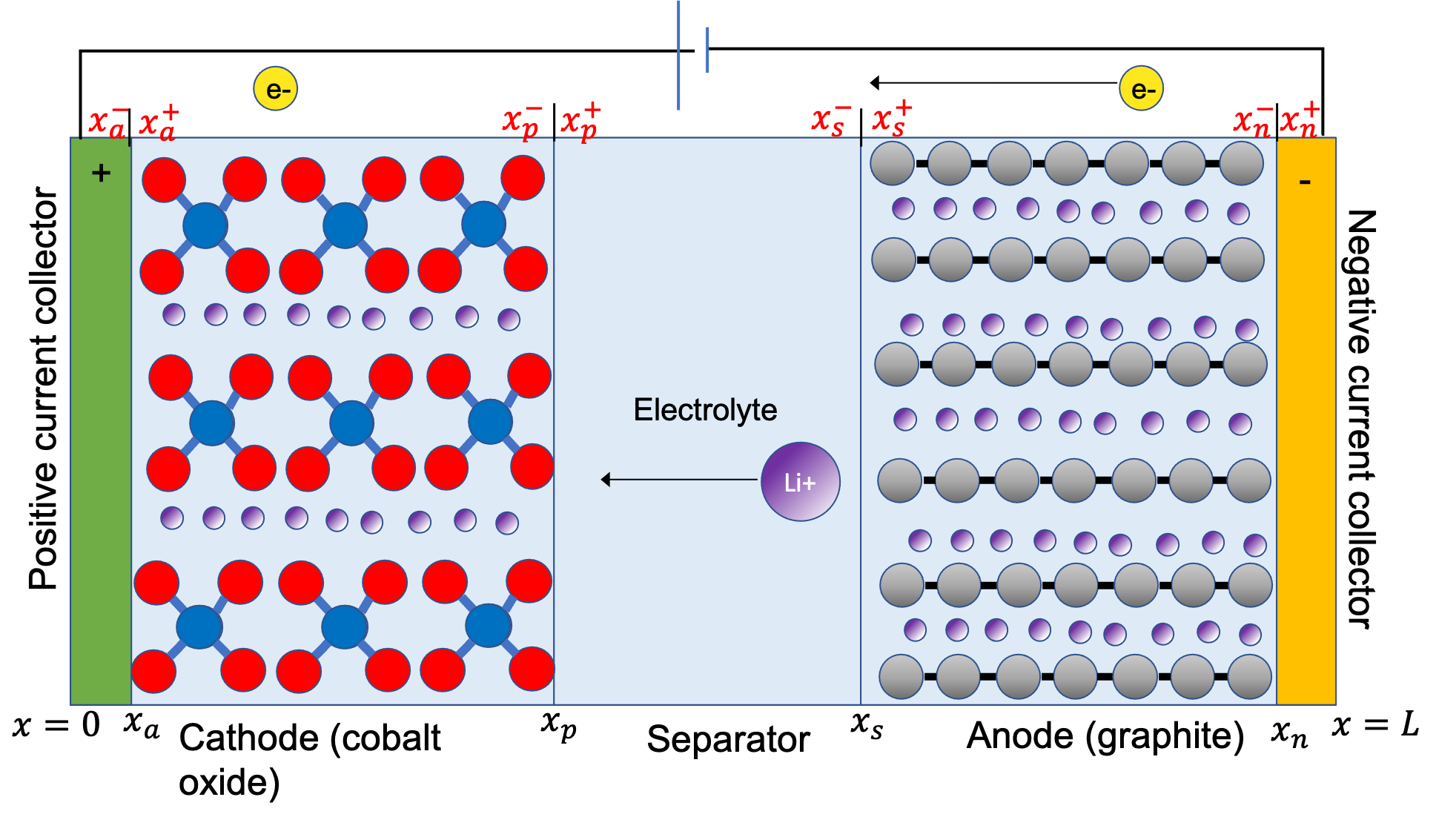
Figure 1: A representation of chemical properties of lithium-ion battery with lithium cobalt oxide and graphite. The purple spheres represent Lithium (Li) that are intercalated in cathode and anode active materials.

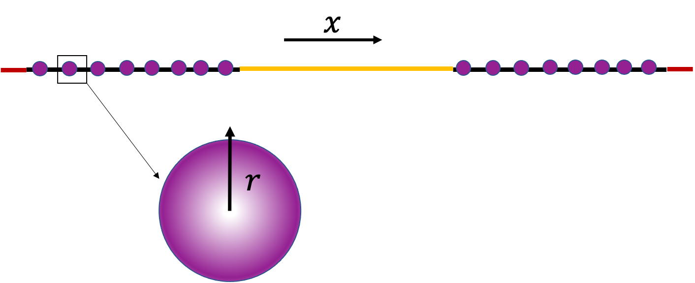
Figure 2: The P2D model abstraction of Figure 1

The P2D model is described by the following quantities: lithium-ion concentrations, potentials, ionic flux across the interface of the spherical particle, current density and temperature. These quantities describe the transport of lithium ion species, conservation of charge, kinetics of charge transfer and thermal behaviour of the battery. The lithium-ion concentrations are denoted by $u(x,t)$ in the electrolyte (liquid phase) and intercalated lithium concentration $c(x,r,t)$ in the solid particle (solid phase). The electric potentials in the liquid and solid phase are $\Phi(x,t)$ and $\Psi(x,t)$ respectively. The interfacial ionic flux is denoted by $j(x,t)$, $I$ is the current density and $T(x,t)$ is the temperature. We take the model form and coefficients from [15]. The governing equations form a PDAE system, where the system is described by partial differential equations and algebraic constraints. We present the form of the equations in detail below, so that the reader can see how we exploit the structure of the nonlinear PDAE to obtain the fast solver.

Throughout the paper, we will use the notation $i\in\{a,p,s,n,z\}$ in subscript to denote the battery section: the positive current collector, cathode, separator, anode and the negative current collector respectively. The ends of the battery are at $x=0$ and $x=L$, where $L$ is the length of the battery. Figure 1 summarizes the domain. The subscript “eff” is used to denote the effective coefficients based on Bruggeman theory [20], which accounts the for varying conductivity or diffusivity due to different materials in composite materials. The model parameters, coefficients and symbols are taken from [15] and also listed in A and B.

2.1 Electrodes and Separator

The intercalation of Li⁺ in the solid particles drive the charge and discharge in Li-ion batteries. The intercalation is driven by diffusion of the lithium concentration,

$$\frac{\partial c}{\partial t}=\frac{1}{r^{2}}\dfrac{\partial}{\partial r}\left(r^{2}D^{s}\frac{\partial c(r,t)}{\partial r}\right),$$ (2.1a)

$$\frac{\partial c(r,t)}{\partial r}\bigg{\rvert}_{r=0}=0,\qquad\frac{\partial c(r,t)}{\partial r}\bigg{\rvert}_{r=R_{p}}=-\frac{j(x,t)}{D^{s}_{\text{eff},i}(T(x,t))}.$$ (2.1b)

Here, $D^{s}$ is a constant solid-phase diffusion coefficient and $D^{s}_{\text{eff},i}$ for $i\in\{p,n\}$ is the effective solid-phase diffusion coefficient which depends on temperature in $x$. The kinetics of charge transfer at the electrodes are described by the Butler-Volmer equation,

$$j(x,t)=2k_{\text{eff}}\sqrt{u(x,t)(c^{\text{max}}_{s,i}-c^{*}(x,t))c^{*}(x,t)}\sinh\left[\dfrac{0.5F}{RT}\eta_{i}(x,t)\right]$$ (2.2)

for $i\in\{p,n\}$, where $\eta_{i}(x,t)$ denotes the overpotential. The equation (2.2) is an algebraic constraint in the PDAE, along with the equation for $\eta_{i}(x,t)$ in (2.10). In the porous electrodes $i\in\{p,n\}$, the accumulation of Li⁺ in the electrolyte phase is described in terms of diffusion of the ions and $j$:

$$\epsilon_{i}\frac{\partial{u(x,t)}}{\partial t}=\frac{\partial}{\partial x}[\mathbf{D_{eff,i}}\frac{\partial u(x,t)}{\partial x}]+a_{i}(1-t_{+})j(x,t),$$ (2.3a)

with equal flux conditions enforced at the boundaries,

$$\frac{\partial u(x,t)}{\partial x}\bigg{\rvert}_{x=\hat{x}_{0},\hat{x}_{n}}=0,$$ (2.3b)

$$-\mathbf{D_{eff,p}}\frac{\partial u(x,t)}{\partial x}\bigg{\rvert}_{x=\hat{x}^{-}_{p}}=-\mathbf{D_{eff,s}}\frac{\partial u(x,t)}{\partial x}\bigg{\rvert}_{x=\hat{x}^{+}_{p}},$$ (2.3c)

$$-\mathbf{D_{eff,s}}\frac{\partial u(x,t)}{\partial x}\bigg{\rvert}_{x=\hat{x}^{-}_{s}}=-\mathbf{D_{eff,n}}\frac{\partial u(x,t)}{\partial x}\bigg{\rvert}_{x=\hat{x}^{+}_{s}}.$$ (2.3d)

The coefficient $\bm{D}_{\text{eff},i}$ is the effective diffusive coefficient of Li⁺ in the electrolyte. The interface positions $\hat{x}_{i}$ are shown in Figure 1.

In the separator where there are no solid particles, we have $j=0$ which yields

$$\epsilon_{i}\frac{\partial u(x,t)}{\partial t}=\frac{\partial}{\partial x}\left[D_{\text{eff},s}\frac{\partial u(x,t)}{\partial x}\right],$$ (2.4a)

with boundary conditions

$$-\bm{D}_{\text{eff},p}\frac{\partial u(x,t)}{\partial x}\rvert_{x=\hat{x}^{-}_{p}}=-\bm{D}_{\text{eff},s}\frac{\partial u(x,t)}{\partial x}\rvert_{x=\hat{x}^{+}_{p}},$$ (2.4b)

$$-\bm{D}_{\text{eff},s}\frac{\partial u(x,t)}{\partial x}\rvert_{x=\hat{x}^{-}_{s}}=-\bm{D}_{\text{eff},n}\frac{\partial u(x,t)}{\partial x}\rvert_{x=\hat{x}^{+}_{s}}.$$ (2.4c)

In the electrodes $i\in\{p,n\}$, the transport of Li⁺ is described by $\Phi$, $T$, $u$ and $j$:

$$a_{i}Fj(x,t)=-\frac{\partial}{\partial x}\left[\mathbf{\kappa_{eff,i}}\frac{\partial\Phi(x,t)}{\partial x}\right]+\frac{\partial}{\partial x}\left[\mathbf{\kappa_{eff,i}}\Upsilon T(x,t)\frac{\partial\ln u(x,t)}{\partial x}\right],$$ (2.5a)

with boundary conditions

$$\frac{\partial\Phi(x,t)}{\partial x}\bigg{\rvert}_{x=\hat{x}_{0}}=0,$$ (2.5b)

$$-\mathbf{\kappa_{eff,p}}\frac{\partial\Phi(x,t)}{\partial x}\bigg{\rvert}_{x=\hat{x}_{p}^{-}}=-\mathbf{\kappa_{eff,s}}\frac{\partial\Phi(x,t)}{\partial x}\bigg{\rvert}_{x=\hat{x}_{p}^{+}},$$ (2.5c)

$$-\mathbf{\kappa_{eff,s}}\frac{\partial\Phi(x,t)}{\partial x}\bigg{\rvert}_{x=\hat{x}_{s}^{-}}=-\mathbf{\kappa_{eff,n}}\frac{\partial\Phi(x,t)}{\partial x}\bigg{\rvert}_{x=\hat{x}_{s}^{+}},$$ (2.5d)

$$\Phi(x,t)\bigg{\rvert}_{x=\hat{x}_{n}}=0,$$ (2.5e)

where $$\bm{\kappa}_{\text{eff},i}$$ is the effective electrolyte phase conductivity.

Again, in the separator, the ionic flux $j$ is $0$. Therefore, the ionic transport in the separator is described by:

$$0=-\frac{\partial}{\partial x}\left[\bm{\kappa}_{\text{eff},s}\frac{\partial\Phi(x,t)}{\partial x}\right]+\frac{\partial}{\partial x}\left[\bm{\kappa}_{\text{eff},s}T(x,t)\Upsilon\frac{\partial\ln u(x,t)}{\partial x}\right]$$ (2.6a)

with boundary conditions

$$-\bm{\kappa}_{\text{eff},p}\frac{\partial\Phi(x,t)}{\partial x}\rvert_{x=\hat{x}^{-}_{p}}=-\bm{\kappa}_{\text{eff},s}\frac{\partial\Phi(x,t)}{\partial x}\rvert_{x=\hat{x}^{+}_{p}},$$ (2.6b)

$$-\bm{\kappa}_{\text{eff},s}\frac{\partial\Phi(x,t)}{\partial x}\rvert_{x=\hat{x}^{-}_{s}}=-\bm{\kappa}_{\text{eff},n}\frac{\partial\Phi(x,t)}{\partial x}\rvert_{x=\hat{x}^{+}_{s}}.$$ (2.6c)

The movement of electrons in the electrodes is governed by Ohm’s law [21], which involves the solid phase potential $\Psi$,

$$\frac{\partial}{\partial x}\left[\mathbf{\sigma_{eff,i}}\frac{\partial\Psi(x,t)}{\partial x}\right]=a_{i}Fj(x,t),$$ (2.7a)

$$\mathbf{\sigma_{eff,i}}\frac{\partial\Psi(x,t)}{\partial x}\bigg{\rvert}_{x=\hat{x}_{0},\hat{x}_{n}}=-I_{\text{app}}(t),\qquad\mathbf{\sigma_{eff,i}}\frac{\partial\Psi(x,t)}{\partial x}\bigg{\rvert}_{x=\hat{x}_{p},\hat{x}_{s}}=0.$$ (2.7b)

For each electrode $i\in\{p,n\}$, $\sigma_{\text{eff},i}$ is the effective solid-phase conductivity and $I_{\text{app}}$ is the applied current.

The heat created in the battery is described by:

$$\rho_{i}C_{p,i}\frac{\partial T(x,t)}{\partial t}=\frac{\partial}{\partial x}\left[\lambda_{i}\frac{\partial T(x,t)}{\partial x}\right]+\bm{Q}_{\text{ohm}}+\bm{Q}_{\text{rxn}}+\bm{Q}_{\text{rev}},$$ (2.8a)

which includes different heat sources. As mentioned in [15], the ohmic generation rate $$\bm{Q}_{\text{ohm}} \bm{Q}_{\text{rxn}} \bm{Q}_{\text{rev}}$$ takes account of heat generated from the movement of Li⁺, the reaction generation rate describes the heat resulting from the ionic flux and overpotentials, and finally the reversible generation rate accounts for the change of entropy in the electrodes. Details of these expressions can be found in the A. The thermal flux continuity interface conditions for temperature are enforced,

$$-\lambda_{z}\frac{\partial T(x,t)}{\partial x}\bigg{\rvert}_{x=\hat{x}_{0}^{-}}=-\lambda_{p}\frac{\partial T(x,t)}{\partial x}\bigg{\rvert}_{x=\hat{x}_{0}^{+}},$$ (2.8b)

$$-\lambda_{n}\frac{\partial T(x,t)}{\partial x}\bigg{\rvert}_{x=\hat{x}_{n}^{-}}=\lambda_{z}\frac{\partial T(x,t)}{\partial x}\bigg{\rvert}_{x=\hat{x}_{n}^{+}}$$ (2.8c)

Similarly, the temperature effects in the separator is described but without $\bm{Q}_{\text{rxn}}$ and $\bm{Q}_{\text{rev}}$:

$$\rho_{i}C_{p,i}\frac{\partial T(x,t)}{\partial t}=\frac{\partial}{\partial x}\left[\lambda_{i}\frac{\partial T(x,t)}{\partial x}\right]+\bm{Q}_{ohm},$$ (2.9a)

$$-\lambda_{p}\frac{\partial T(x,t)}{\partial x}\rvert_{x=\hat{x}^{-}_{p}}=-\lambda_{s}\frac{\partial T(x,t)}{\partial x}\rvert_{x=\hat{x}^{+}_{p}},$$ (2.9b)

$$-\lambda_{s}\frac{\partial T(x,t)}{\partial x}\rvert_{x=\hat{x}^{-}_{s}}=-\lambda_{n}\frac{\partial T(x,t)}{\partial x}\rvert_{x=\hat{x}^{+}_{s}}.$$ (2.9c)

Lastly, we give an equation for the surface overpotential $\eta(x,t)$ of the electrode $i\in\{p,n\}$:

$$\eta_{i}(x,t)=\Psi(x,t)-\Phi(x,t)-\mathbf{U_{i}}(T(x,t),c(x,r,t))$$ (2.10)

where $\mathbf{U_{i}}$ is the open circuit potential which is fitted experimentally (see A).

2.2 Current Collectors

The current collectors consist of conductive metal materials for transfer of electrons. We model the thermal effects in these regions:

$$\rho_{i}C_{p,i}\frac{\partial T(x,t)}{\partial t}=\frac{\partial}{\partial x}\left(\lambda_{i}\frac{\partial T(x,t)}{\partial x}\right)+\frac{I^{2}_{app}(t)}{\sigma_{\text{eff},i}},$$ (2.11a)

with boundary conditions

$$-\lambda_{a}\frac{\partial T(x,t)}{\partial x}\rvert_{x=0} =h(T_{ref}-T(x,t)),$$ (2.11b)

$$-\lambda_{z}\frac{\partial T(x,t)}{\partial x}\rvert_{x=L} =h(T(x,t)-T_{ref}),$$ (2.11c)

with heat exchange coefficient $h$. The boundary conditions represent Newton’s law of cooling at the two ends of the battery, with ambient temperature $T_{ref}$.

3 Implementation

The system of equations in Section 2 is discretised in space by cell centred finite differences, and in time using backward Euler method for the time-dependent variables, $u(x,t)$, $c(x,r,t)$ and $T(x,t)$. The complete discretizations are given in Tables 1 and 2. We describe the structure of the discrete nonlinear system below.

3.1 Solving the nonlinear system

We first describe how to solve the resulting nonlinear system from the PDAE without considering the specific structure of the problem. We will call this basic implementation as naïve method. After discretising in space, we obtain a set of differential algebraic equations (DAE). In particular, we obtain a semi-explicit index-1 DAE, where one can distinguish the differential and algebraic variables. Variables without time derivatives are called algebraic as in standard PDAE literature [22]. We denote the discrete versions of the electrochemical quantities $c(x,r,t),j(x,t),u(x,t),\Phi(x,t),\Psi(x,t),T(x,t)$ and $\eta(x,t)$ as

$$\bm{c} =(c_{p},c_{n}),\quad\bm{j}=(j_{p},j_{n}),\quad\bm{u}=(u_{p},u_{s},u_{n}),$$

$$\bm{\Phi} =(\Phi_{p},\Psi,\Phi_{n}),\quad\bm{\Psi}=(\Psi_{p},\Psi,_{n}),$$

$$\bm{T} =(T_{a},T_{p},T_{s},T_{n},T_{z}),\quad\bm{\eta}=(\eta_{p},\eta_{n}).$$

We can group the differential variables in $x$ as $\hat{U}=[\bm{u},\bm{T}]$ and algebraic variables as $\tilde{U}=[\bm{\Phi},\bm{\Psi},\bm{j},\bm{\eta}]$. The solid particle concentration $\bm{c}$ is also a differential variable in $r$. After discretising in time using backward Euler, we form the following set of nonlinear equations,

$$\bm{0} =\bm{c}^{k}-\Delta t\bm{G}(\bm{c}^{k},\hat{U}^{k},\tilde{U}^{k})-\bm{c}^{k-1}$$ (3.1a)

$$\bm{0} =\hat{U}^{k}-\Delta t\bm{\hat{F}}(\bm{c}^{k},\hat{U}^{k},\tilde{U}^{k})-\hat{U}^{k-1}$$ (3.1b)

$$\bm{0} =\bm{\tilde{F}}(\bm{c}^{k},\hat{U}^{k},\tilde{U}^{k}),$$ (3.1c)

where $k$ denotes the time step. From (3.1), we form a larger multi-dimensional vector valued function $\bm{F}(U)$, where $U$ is the aggregate vector containing all the unknowns,

$$\begin{split}U&=[\begin{matrix}c_{p}&c_{n}&u_{p}&u_{s}&u_{n}&j_{p}&j_{n}&\eta_{p}&\eta_{n}\end{matrix}\\ &\qquad\qquad\begin{matrix}\Phi_{p}&\Psi&\Phi_{n}&\Psi_{p}&\Psi_{n}&T_{a}&T_{p}&T_{s}&T_{n}&T_{z}\end{matrix}]^{T}.\end{split}$$ (3.2)

Solving for (3.1) is equivalent to finding the root of the function

$$\bm{F}(U^{k})=\bm{0}$$ (3.3)

at every $k$th time step. We solve for the root of (3.3) iteratively using Newton’s iteration,

$$U^{p+1}=U^{p}-[\mathcal{J}^{-1}(U^{p})]\bm{F}(U^{p})$$ (3.4)

where $p$ denotes the $p$th iterate of the Newton’s method and $\mathcal{J}$ is the Jacobian of $\bm{F}$ at $U^{p}$. Solving for the inverse of $\mathcal{J}(U^{p})$ is computationally expensive, especially when we have a large system. Therefore, we use a linear solver to solve for $\delta^{p}=[\mathcal{J}^{-1}(U^{p})]\bm{F}(U^{p})$,

$$\mathcal{J}(U)\delta^{p}=\bm{F}(U^{p}).$$ (3.5)

We generate the iterates $U^{p+1}$ by

$$U^{p+1}=U^{p}-\delta^{p}$$ (3.6)

at every iteration until we converge to the root. In this way, we can approximate the solution to PDAE by repeatedly solving large linear systems.

To give an idea of the size of the nonlinear system in this application, we outline the number of unknowns. In each battery section $i\in\{p,n\}$, there are $M_{i}$ points in $x$. For each point in $x$, there are $N_{i}$ points in $r$. Then, the unknowns representing the solid-phase concentration $\bm{c}$ has $M_{p}(N_{p}+2)+M_{n}(N_{n}+2)$ points, where $N_{i}+2$ accounts for the ghost points [23] needed to impose boundary conditions at $r=0$ and $r=R_{p}$. Similarly, each of $u_{p},u_{s}$ and $u_{n}$ has $M_{p}+2$, $M_{s}+2$ and $M_{n}+2$ unknowns respectively, and the same applies for the unknowns $\bm{\Phi}$ and $\bm{T}$. For $\bm{j}$ and $\bm{\eta}$, there are $M_{p}$ and $M_{n}$ points respectively in the positive and negative electrode, since there are no boundary conditions for these variables. In total, there are

$$M_{p}(N_{p}+2)+M_{n}(N_{n}+2)+3(M_{p}+M_{s}+M_{n}+6)+(M_{p}+M_{n}+4)+2(M_{p}+M_{n})$$

unknowns. For example, when we set the number of grid points in each battery section and for each solid particle to be $M=N=30$, we have $2456$ unknowns in the resulting system. The number grows quadratically because of the dimension $r$ of the particles. This emphasizes the need for fast and robust solver for the full P2D model. The main contribution of this work is a fast solver strategy to the linear systems using some of the special structure of the discretised P2D model. For speed and robustness, we also need to consider how to efficiently construct the Jacobians in Newton iterations.

3.2 Automatic-differentiation for Jacobians

The fastest method of computing the Jacobian is to manually differentiate the function components with respect to every element in $U^{p}$ a priori. Then, the cost of computation is just the function evaluation of the differentiated components. This can be done for relatively simple models. However, for the fully-coupled P2D model, manual differentiation is inconvenient due to complex equations and prone to errors in the implementation. As alternatives, one can use numerical, symbolic or automatic differentiation (AD). Numerical differentiation, which involves finite differences, is easy to implement and fast. With numerical differentiation, we must choose the step size $h$ which is especially difficult for systems with multiple scales. We refer the readers to [24] for the details on how round-off and truncation errors depend on the step size $h$.

On the other hand, symbolic and automatic differentiation (AD) compute exact Jacobians. Software for AD records every operation done on the inputs of a function, then builds a graph that encodes all the operations [25]. Then the rules of differentiation are applied on every node of the graph. Symbolic differentiation produces a full expression for the derivative, then the numerical values are substituted. This approach, however, has a problem of expression swell causing slower performance, as pointed out by [25]. We use AD for better performance, which uses intermediate values of computations to calculate the derivatives on the fly. There are two ways to do this, the forward and reverse mode AD. For functions $f:\mathbb{R}^{n}\rightarrow\mathbb{R}^{m}$ where $n>m$, the reverse mode is preferred because the Jacobian can be constructed in $m$ passes but also uses additional space. In contrast, the forward mode is preferred for when $m>n$ because it takes $n$ passes to build the Jacobian. When $m=n$, as is the case for our system, the forward mode is usually preferred due to the large memory usage with the reverse mode. However, in Section 4.2, we show how we can use the backward mode AD to efficiently build the Jacobians. For further details on how AD works, we refer the reader to [25]. Note that the use of symbolic/automatic differentiation allows changes in terms in the equations (effective diffusivity expressions, for example) with no user effort needed to modify the Jacobian.

A particular AD software that is suitable for the Python environment is a library named JAX [19], which we use extensively in our implementation. Section 4.2 discusses how JAX gives an extra performance boost.

Table 1: Discretisation of PDAE from Section 2

Electrodes, $i\in\{p,n\}$

Solid phase concentration    $\displaystyle 0=c^{k-1}_{n,m}-c^{k}_{n,m}+D^{s}\left[\frac{1}{r_{n}^{2}}\left(\frac{r_{n+1/2}^{2}\frac{c^{k}_{n+1,m}-c^{k}_{n,m}}{\Delta r}-r_{n-1/2}^{2}\frac{c^{k}_{n,m}-c^{k}_{n-1,m}}{\Delta r}}{\Delta r}\right)\right],$

$\displaystyle\qquad\frac{c^{k}_{1,m}-c^{k}_{0,m}}{\Delta r}=0,\qquad\frac{c^{k}_{N+1,m}-c^{k}_{N,m}}{\Delta r}+\frac{j^{k}_{m}}{D^{s}_{\text{eff}}}=0.$

Electrolyte concentration    $\displaystyle 0=u^{k-1}_{m}-u^{k}_{m}-\frac{\Delta t}{\epsilon_{i}}\left(\frac{{D_{\text{eff},m}}^{r}(u^{k}_{m+1}-u^{k}_{m})}{\Delta x^{2}}-\frac{{D_{\text{eff},m}}^{l}(u^{k}_{m}-u^{k}_{m-1})}{\Delta x^{2}}+a_{i}(1-t_{+})j^{k}_{m}\right),$

$\displaystyle\frac{u^{k}_{p_{1}}-u^{k}_{p_{0}}}{\Delta x_{p}}=0,\qquad\frac{u^{k}_{n_{M_{n}+1}}-u^{k}_{n_{M_{n}}}}{\Delta x_{n}}=0$,

$\displaystyle\frac{u^{k}_{p_{M_{p}}}+u^{k}_{p_{M_{p}+1}}}{2}=\frac{u^{k}_{s_{0}}+u^{k}_{s_{1}}}{2},\qquad\frac{u^{k}_{s_{M_{s}}}+u^{k}_{s_{M_{s+1}}}}{2}=\frac{u^{k}_{n_{0}}+u^{k}_{n_{1}}}{2}$.

Electrolyte potential    $\displaystyle a_{i}Fj^{k}_{m}+(\kappa^{r}_{\text{eff}}\frac{\Phi^{k}_{m+1}-\Phi^{k}_{m}}{\Delta x^{2}}-\kappa^{l}_{\text{eff}}\frac{\Phi^{k}_{m}-\Phi^{k}_{m-1}}{\Delta x^{2}})-\gamma(\kappa^{r}_{\text{eff}}T^{k}_{m+1}\frac{\ln{u^{k}_{m+1}-\ln{u^{k}_{m}}}}{\Delta x^{2}})$

$\displaystyle\frac{\Phi_{{p_{1}}}-\Phi_{{p_{0}}}}{\Delta x}=0,\qquad\frac{\Phi_{n_{N}}+\Phi_{n_{N+1}}}{2}=0,$

$\displaystyle\frac{\Phi^{k}_{p_{M_{p}}}+\Phi^{k}_{p_{M_{p}+1}}}{2}=\frac{\Phi^{k}_{s_{0}}+\Phi^{k}_{s_{1}}}{2},\qquad\frac{\Phi^{k}_{s_{M_{s}}}+\Phi^{k}_{s_{M_{s+1}}}}{2}=\frac{\Phi^{k}_{n_{0}}+\Phi^{k}_{n_{1}}}{2}$.

Solid phase potential    $\displaystyle\sigma_{\text{eff},i}\frac{\Psi^{k}_{m+1}-2\Psi^{k}_{m}+\Psi^{k}_{m-1}}{\Delta x_{i}^{2}}=0,$

$\displaystyle\sigma_{\text{eff},p}\frac{\Psi^{k}_{p_{1}}-\Psi^{k}_{p_{0}}}{\Delta x_{p}}=-I_{app},\qquad\sigma_{\text{eff},p}\frac{\Psi^{k}_{p_{M_{p}+1}}-\Psi^{k}_{p_{M_{p}}}}{\Delta x_{p}}=0,$

$\displaystyle\sigma_{\text{eff},n}\frac{\Psi^{k}_{n_{1}}-\Psi^{k}_{n_{0}}}{\Delta x_{n}}=0,\qquad\sigma_{\text{eff},n}\frac{\Psi^{k}_{n_{M_{n}+1}}-\Psi^{k}_{n_{M_{n}}}}{\Delta x_{n}}=0.$

Table 2: Discretisation of PDAE from Section 2

Electrodes, $i\in\{p,n\}$

Temperature    $\displaystyle\rho_{i}C_{p,i}\frac{T^{k}_{m}-T^{k-1}_{m}}{\Delta t}-\left(\lambda_{i}\left[\frac{T^{k}_{m+1}-2T^{k}_{m}+T^{k}_{m-1}}{\Delta x^{2}}\right]+Q_{ohm}+Q_{rxn}+Q_{rev}\right)=0,$

$\displaystyle-\lambda_{a}\frac{T^{k}_{a_{M_{a}+1}}-T^{k}_{a_{M_{a}}}}{\Delta x_{a}}=-\lambda_{p}\frac{T^{k}_{p_{1}}-T^{k}_{p_{0}}}{\Delta x_{p}},\qquad-\lambda_{n}\frac{T^{k}_{n_{M_{n}+1}}-T^{k}_{n_{M_{n}}}}{\Delta x_{n}}=-\lambda_{z}\frac{T^{k}_{z_{1}}-T^{k}_{z_{0}}}{\Delta x_{z}}.$

$\displaystyle\frac{T^{k}_{p_{M_{p}}}+T^{k}_{p_{M_{p}+1}}}{2}=\frac{T^{k}_{s_{0}}+T^{k}_{s_{1}}}{2},\qquad\frac{T^{k}_{s_{M_{s}}}+T^{k}_{s_{M_{s+1}}}}{2}=\frac{T^{k}_{n_{0}}+T^{k}_{n_{1}}}{2}$.

Ionic flux    $\displaystyle j^{k}_{m}-2_{k_{\text{eff}},i}\sqrt{u^{k}_{m}(c^{max}-c^{*k}_{m})c^{*k}_{m}}\sinh{\frac{0.5F}{RT^{k}_{m}}\eta^{k}_{m}=0}$

Overpotential    $\displaystyle\eta^{k}_{m}-\Psi^{k}_{m}+\Phi^{k}_{m}-U_{i}=0$

Current collectors, $i\in\{a,z\}$

Temperature    $\displaystyle\rho_{i}C_{p,i}\frac{T^{k}_{m+1}-T^{k}_{m}}{\Delta t}-\left(\lambda_{i}\left[\frac{T^{k}_{m+1}-2T^{k}_{m}+T^{k}_{m-1}}{\Delta x^{2}}\right]+\frac{I^{2}_{app}}{\sigma_{\text{eff},i}}\right)=0,$

$\displaystyle-\lambda_{a}\frac{T^{k}_{a_{1}}-T^{k}_{a_{0}}}{\Delta x_{a}}=h(T_{ref}-T^{k}_{a_{1/2}}),\qquad-\lambda_{z}\frac{T^{k}_{z_{M_{z}+1}}-T^{k}_{z_{M_{z}}}}{\Delta x_{z}}=h(T^{k}_{z_{M_{z}+1/2}}-T_{ref}).$

Separator, $i=s$

Electrolyte concentration    $\displaystyle 0=u^{k-1}_{m}-u^{k}_{m}-\frac{\Delta t}{\epsilon_{i}}\left(\frac{{D_{\text{eff},m}}^{r}(u^{k}_{m+1}-u^{k}_{m})}{\Delta x^{2}}-\frac{{D_{\text{eff},m}}^{l}(u^{k}_{m}-u^{k}_{m-1})}{\Delta x^{2}}\right),$

$\displaystyle-D^{r}_{\text{eff},p_{M_{p}}}\frac{u_{M_{p}+1}-u_{M_{p}}}{\Delta x_{p}}=-D^{r}_{\text{eff},s_{0}}\frac{u_{s_{1}}-u_{s_{0}}}{\Delta x_{s}},\qquad-D^{r}_{\text{eff},s_{M_{s}}}\frac{u_{M_{s}+1}-u_{M_{s}}}{\Delta x}=-D^{r}_{\text{eff},n_{0}}\frac{u_{n_{1}}-u_{n_{0}}}{\Delta x_{n}}.$

Electrolyte potential    $\displaystyle-(\kappa^{r}_{\text{eff}}\frac{\Phi^{k}_{m+1}-\Phi^{k}_{m}}{\Delta x^{2}}-\kappa^{l}_{\text{eff}}\frac{\Phi^{k}_{m}-\Phi^{k}_{m-1}}{\Delta x^{2}})+\gamma(\kappa^{r}_{\text{eff}}T^{k}_{m+1}\frac{\ln{u^{k}_{m+1}-\ln{u^{k}_{m}}}}{\Delta x^{2}})=0,$

$\displaystyle-\kappa^{r}_{\text{eff},p_{M_{p}}}\frac{\Phi_{M_{p}+1}-\Phi_{M_{p}}}{\Delta x_{p}}=-\kappa^{r}_{\text{eff},s_{0}}\frac{\Phi_{s_{1}}-\Phi_{s_{0}}}{\Delta x_{s}},\qquad-\kappa^{r}_{\text{eff},s_{M_{s}}}\frac{\Phi_{M_{s}+1}-\Phi_{M_{s}}}{\Delta x_{s}}=-D^{r}_{\text{eff},n_{0}}\frac{u_{n_{1}}-u_{n_{0}}}{\Delta x_{n}}.$

Temperature    $\displaystyle\rho_{i}C_{p,i}\frac{T^{k+1}_{m}-T^{k}_{m}}{\Delta t}-\left(\lambda_{i}\left[\frac{T^{k}_{m+1}-2T^{k}_{m}+T^{k}_{m-1}}{\Delta x^{2}}\right]+Q_{ohm}\right)=0,$

$\displaystyle-\lambda_{p}\frac{T^{k}_{p_{M_{p}+1}}-T^{k}_{p_{M_{p}}}}{\Delta x_{p}}=-\lambda_{s}\frac{T^{k}_{s_{1}}-T^{k}_{s_{0}}}{\Delta x_{s}},\qquad-\lambda_{n}\frac{T^{k}_{s_{1}}-T^{k}_{s_{0}}}{\Delta x_{s}}=-\lambda_{n}\frac{T^{k}_{n_{M_{n}+1}}-T^{k}_{n_{M_{n}}}}{\Delta x_{n}}.$

4 Decoupled method

As mentioned in Section 3.1, the major bottleneck of the computation comes from solving the linear system

$$\mathcal{J}(U^{p})\delta=\bm{F}(U^{p})$$ (4.1)

at every Newton iteration at every time step. $\mathcal{J}$ is of size $\mathcal{O}(NM)\times\mathcal{O}(NM)$. In this section, we present a decoupled method to solve the linear system in two steps which results in a smaller Jacobian matrix of size $\mathcal{O}(M)\times\mathcal{O}(M)$. We do this by decoupling the equation for $\bm{c}$ from $\bm{F}(U)$. The technique results in an exact solve without any approximations. This way, we can reduce the computation cost of solving the linear system at every Newton iteration. From (2.1) we see that equation for lithium-ion concentration $c$ is linear except at the boundary of the sphere $r=R_{p}$. Writing the discretised (2.1) in a matrix form, we obtain

$$A\bm{c_{m}}^{k}=\begin{bmatrix}0\\ c_{1,m}^{k-1}\\ \vdots\\ c_{N,m}^{k-1}\\ 0\end{bmatrix}-\frac{j_{m}^{k}}{D^{s}_{eff}(T^{k}_{m})}\begin{bmatrix}0\\ 0\\ \vdots\\ 0\\ 1\end{bmatrix},$$ (4.2)

where $\bm{c}^{k}_{m}$ is the particle equation at point $x_{m}$; therefore, for each $m=1,2,\dots,M$, we would have to solve (4.2). Without the decoupling, which will be described shortly, (4.2) is solved as part of the larger system, as it is coupled to every other variable through $j$. $A$ is the tridiagonal coefficient matrix for and $\bm{c}^{k}_{m}$. Let $a_{n}=\frac{-D^{s}\Delta t}{r^{2}_{n}\Delta r^{2}}r^{2}_{n-1/2}$, $b_{n}=1+\frac{D^{s}\Delta t}{r^{2}_{n}\Delta r^{2}}$, $c_{n}=\frac{-D^{s}\Delta t}{r^{2}_{n}\Delta r^{2}}r^{2}_{n+1/2}$. Then,

$$A=\begin{pmatrix}-1&1&0&0&0&\dots&0\\ 0&a_{1}&b_{1}&c_{1}&0&\dots&0\\ 0&0&a_{2}&b_{2}&c_{2}&\dots&0\\ \vdots&\vdots&\ddots&\ddots&\ddots&\ldots&\vdots\\ 0&0&\ldots&\ldots&\ldots&\frac{-1}{\Delta r}&\frac{1}{\Delta r}\end{pmatrix}.$$ (4.3)

We now show how the system can be decoupled. Rearranging (4.2), we can split $\bm{c}^{k}_{m}$ into two parts

$$\bm{c}^{k}_{I_{m}}=A^{-1}\begin{bmatrix}0&c^{k-1}_{0,m}&\ldots&c_{N,m}^{k-1}&0\end{bmatrix}^{T},$$

$$\bm{c}^{k}_{II_{m}}=\frac{j_{m}^{k}}{D_{s}(T^{k}_{m})}A^{-1}\begin{bmatrix}0&0&\ldots&0&1\end{bmatrix}^{T}.$$

The constant vector $A^{-1}\begin{bmatrix}0&0&\ldots&0&1\end{bmatrix}^{T}$ in $\bm{c}^{k}_{II_{m}}$, which we denote $\gamma$, is a vector that can be precomputed once. By formulating as such, we have partially decoupled the particle equations from the whole system. This is because we can compute $\bm{c}^{k}_{I_{m}}$ by solving

$$A\bm{c}^{k}_{I_{m}}=\begin{bmatrix}0\\ c_{1,m}^{k-1}\\ \vdots\\ c_{N,m}^{k-1}\\ 0\end{bmatrix}$$ (4.4)

cheaply via tridiagonal LU factorisation. Thus, we avoid the full $\mathcal{O}(NM)\times\mathcal{O}(NM)$ Jacobian of $F(U)$. The vector $\bm{c}^{k}_{II_{m}}$ can be obtained by scalar-vector multiplication once we have a solution for $\bm{j}$ and $\bm{T}$. Equations that are functions of $\bm{c}$, (2.2), (2.8) and (2.10), only require the interfacial concentration $c^{*}(x,t)$. In our original system, $c^{*}$ is approximated as

$$c^{*}(x_{m},t)\approx c^{*^{k}}_{m} =\frac{c^{k}_{N,m}+c^{k}_{N+1,m}}{2}.$$

This can be rewritten as

$$c^{*^{k}}_{m} =\underbrace{\frac{c^{k}_{1_{N,m}}+c^{k}_{1_{N+1,m}}}{2}}_{\textstyle=\alpha^{k}_{m}}-\frac{j^{k}_{m}}{D^{s}_{\text{eff}}(T^{k}_{m})}\underbrace{\frac{\gamma_{N+1}+\gamma_{N}}{2}}_{\textstyle=\beta}.$$

Treating $\alpha^{k}_{m}$ and $\beta$ as constants, $c^{*}(x,t)$ is a function of $j$ and $T$, $c^{*k}_{m}=\alpha^{k}_{m}-\frac{j^{k}_{m}}{D^{s}(T^{k}_{m})}\beta$. In this way, none of the channel equations depend explicitly on variable $\bm{c}$. Therefore, $\bm{c}$ does not need to be computed in the Newton iterations. We can proceed with the Newton iteration with $U=(\bm{u},\bm{j},\bm{\eta},\bm{T}\bm{\phi},\bm{\psi})$ where we solve a linear system of a $\mathcal{O}(M)\times\mathcal{O}(M)$ matrix. Table 3 compares the size of the Jacobian for each method. We stress here that the decoupled method solves the same system as the naïve method. We obtain the same solution to machine precision. If there is a nonlinear dependence in the particle diffusion, the decoupling will still apply, although the tridiagonal solves (4.4) for each particle will need to be updated at each Newton step.

In Section 4.1, we further improve the efficiency by reordering the entries of Jacobian and computing only the nonzero entries of the reduced Jacobian.

$N_{p}=N_{n}$	$M_{p}=M_{n}$	$M_{s}=M_{a}=M_{z}$	$N_{\text{jac}}$: naive	$N_{\text{jac}}$: decoupled
10	10	5	411	171
20	20	5	1171	291
30	30	5	2331	411
40	40	5	3891	531
50	50	5	5851	651

Table 3: The table shows the size of the Jacobian for each method at different resolutions. The same number of grid points in $r$ and $x$ for positive and negative electrode was used. The number of grid points was set fixed to $5$ in the separator, positive and negative current collector. The size of the Jacobian grows by $\mathcal{O}(NM)$ for the naive method, whereas only $\mathcal{O}(M)$ for decoupled.

4.1 Reordering the Jacobian

The vector $U$ from our decoupled system can be reordered such that the Jacobian is a banded diagonal matrix. By reordering, we can use an appropriate banded linear solver to enhance the performance. We rearrange $U$ in an alternating fashion,

$$\begin{split}U&=[\begin{matrix}\bm{u}_{p}&\bm{u}_{s}&\bm{u}_{n}&\bm{j}_{p}&\bm{j}_{n}&\bm{\eta}_{p}&\bm{\eta}_{n}\end{matrix}\\ &\qquad\qquad\begin{matrix}\bm{\Psi}_{p}&\bm{\Psi}_{n}&\bm{\Phi}_{p}&\bm{\Phi}_{s}&\bm{\Phi}_{n}&\bm{T}_{a}&\bm{T}_{p}&\bm{T}_{s}&\bm{T}_{n}&\bm{T}_{z}\end{matrix}]^{T}\end{split}$$ (4.5)

$$\downarrow$$

$$\begin{split}U_{r}&=[\begin{matrix}\bm{T}_{a}&{u}_{p_{0}}&{\Psi}_{p_{0}}&{\Phi}_{p_{0}}&{T}_{p_{0}}\end{matrix}\\ &\qquad\qquad\begin{matrix}u_{p_{1}}&j_{p_{0}}&\eta_{p_{0}}&\Phi_{s_{p_{1}}}&\Phi_{e_{p_{1}}}&T_{p_{1}}&u_{p_{2}}\cdots&T_{p_{Mp}}\end{matrix}\\ &\qquad\qquad\qquad\begin{matrix}{u}_{p_{Mp+1}}{\Psi}_{p_{Mp+1}}&{\Phi}_{p_{Mp+1}}&{T}_{p_{Mp+1}}\end{matrix}\\ &\qquad\qquad\qquad\qquad\begin{matrix}{u}_{s_{0}}&{\Phi}_{s_{0}}&{T}_{s_{0}}&u_{s_{1}}&\Phi_{e_{s_{1}}}&T_{s_{1}}&\cdots&{u}_{s_{Ms+1}}&{\Phi}_{s_{Ms+1}}&{T}_{s_{Ms+1}}\end{matrix}\\ &\qquad\qquad\qquad\qquad\qquad\begin{matrix}\cdots&u_{n_{1}}&j_{n_{0}}&\eta_{n_{0}}&\Phi_{s_{n_{1}}}&\Phi_{e_{n_{1}}}&T_{n_{1}}&\cdots&\bm{T}_{z}\end{matrix}]^{T}\end{split}$$ (4.6)

The variables are ordered such that $u_{i},j_{i},\eta_{i},\Psi_{i},\Phi_{i}$ and $T_{i}$ at each $i-$th grid point are next to each other, rather than the original set up described in (3.2). Figure 3 illustrates how the sparsity pattern of the Jacobian changes.

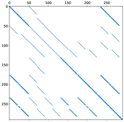
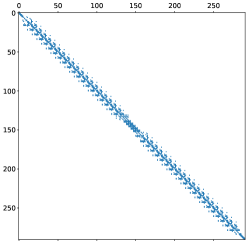
Figure 3: The sparsity pattern of Jacobian from the unordered system on the left. On the right is the sparsity pattern after the Jacobian is reordered.

Banded matrix

The reordered Jacobian, which we denote by $\mathcal{J}_{r}$, can be stored in a diagonal ordered form. There are $23$ nonzero lower and $23$ upper diagonals in $\mathcal{J}_{r}$. Then, $\mathcal{J}_{r}$ can be represented as a matrix of size $(23+23+1)\times N_{tot}$ where $N_{tot}$ is the size of $U$. We denote this banded matrix by $\mathcal{J}_{b}$. The entries are stored in the following way,

$$\mathcal{J}_{b}[u+i-j,j]=\mathcal{J}_{r}[i,j],\quad i=0,1,\cdots,(l+u),\quad j=0,1,\cdots,N_{tot}.$$

The number of rows in $\mathcal{J}_{b}$ is fixed for a given model, as the number of rows correspond to the number of partial derivatives in the system. $\mathcal{J}_{b}$ is passed to the banded linear solver, which uses $LU$ decomposition to solve the linear system.

4.2 Constructing the Jacobian

We describe some of the performance gains that can be achieved by using JAX in Python. JAX is especially useful for high-performance computations because it uses a domain-specific compiler XLA (Accelerated Linear Algebra) that can optimize computations at a lower level with improved memory usage and speed. Compiling code just-in-time (jit) via XLA in Python accelerates the performance because the source code is directly compiled to machine code as the program runs. This is often faster than interpreting, which is typical for languages like Python, making the performance comparable to that of compiled languages like C. The readers can refer to [19] and [26] for more information.

In our problem, a fast compiler that optimizes differentiation computation is very useful because we need to compute the system Jacobian at $U$ at every Newton step. In addition to differentiation, the compiler can speed up any array manipulations. Any functions that are compiled using XLA incur initial overhead when first called, and is cached to be used later. This is useful for functions that are called many times, as is the case in our problem with multiple Newton updates and time stepping. For example, the first time we build the Jacobian, there is an overhead of roughly 15 seconds (independent of the size of the vector). The proceeding computations are fast.

However, there are limitations of using JAX’s built-in forward-mode Jacobian function. While JAX can automatically output the Jacobian when $U$ is fed into its built-in function, the output is dense. Currently, the sparse output of Jacobians is not supported. This creates an extra overhead of converting the matrix into a sparse form to use sparse linear solvers. This drawback also causes a computational bottleneck. The evaluation of Jacobian with JAX’s built-in function is quite costly for large vectors, even when compiled with XLA. This is likely coming from the redundant computation effort computing partial derivatives that evaluate to zeros. By the method discussed in Sections 4.1, we bypass this problem by directly constructing the banded reordered Jacobian, $\mathcal{J}_{b}$, without using JAX’s built-in Jacobian function.

For each discretised PDE equation, we take the partial derivatives with respect to their arguments via backward mode AD on a scalar level ($\mathbb{R}^{\text{Ntot}}\rightarrow\mathbb{R}$). This avoids computing redundant zeros. Many of the discretised equations are repeated over the grid points, but they can be vectorized. We predetermine the sparsity of $\mathcal{J}_{b}$ prior to the simulation, which is unique to the reordering scheme and the model. At each Newton update, we populate the matrix with partial derivatives with the predetermined sparsity. The array update process is sped up by compilation via XLA. This method provides an efficient way constructing the Jacobian that takes advantage of the tools provided by JAX.

5 Experimental setup

All simulations were done on Mac CPU, with 3.5 GHz Dual-Core Intel Core i7 processor and 8GB RAM, in Python. Our code is freely available on Github at https://github.com/hanrach/p2d_fast_solver. We ran the simulations until the full battery discharge at $1$C, which is observed at $t=3620$ seconds. At the current collectors and the separator, coarse grids ($M_{a},M_{s},M_{z}=5$) were used for speed, because of the simpler governing equations in those sections. We varied the grid sizes in the electrodes, with same number of grid points at each positive and negative electrode in $x$ and $r$ ($M_{p}=N_{p}=M_{n}=N_{n}$). The time step in the backward Euler method was fixed to $\Delta t=10$.

5.1 Voltage curves under different C rates

We experimentally validate our solver by comparing the voltage curves against Figure 9 in [15]. We run the simulation until the full discharge at different C rates with the heat exchange coefficient $h$ fixed to $1$W/(m²K). We plot how the average temperature and the battery voltage changes over time in Figure 4. The battery voltage is defined as the difference in solid phase potential at the two ends of the electrodes, $V=\Psi_{p_{0}}-\Psi_{n_{M_{n}}}$. As expected, at higher C rates the temperature rises rapidly and the voltage drops quickly to the cut-off voltage of $2.5$V. These figures are qualitatively similar to Figure 9 in [15]. The script examples/different_C_rates.py was used to generate Figure 4.

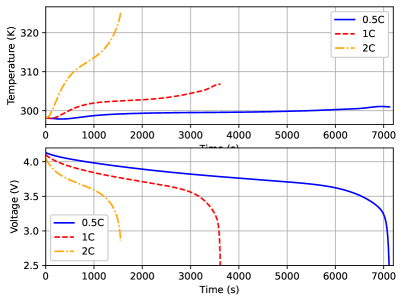
Figure 4: Temperature and voltage changes during the discharge cycle under 0.5C, 1C and 2C.

5.2 Comparsion between the naïve method and the fast solver

We compare the performance between the naïve method, which does not include the decoupling and uses the built-in Jacobian function in JAX, and the fast method where we decouple $c$ as well as construct the Jacobian in a diagonal ordered form directly. When solving the linear system $J\delta^{p}=\mathbf{U}^{p}$ for the naïve method, we convert the dense Jacobian into a sparse matrix and apply a generic sparse linear solver. Table 4 summarizes the methods.

	Decoupled	Jacobian Function	Linear Solver
Naïve	No	JAX	Generic sparse
Fast	Yes	Custom	Tridiagonal and banded

Table 4: The fast method improves upon the naïve method by decoupling the solid particle equations from the electrolyte equations, and employing the custom Jacobian function and linear solvers that exploit the structure of the matrices.

Figure 5 compares the cumulative time spent on solving the linear systems within the Newton iterations. The overhead of conversion for the naïve method is not costly compared to the actual time to solve the linear systems. This factor is not included in the measurements in Figure 5. At a moderately fine grid $M=30$, the naïve method spends a total of about $3.5$ seconds. The fast solver is roughly $12$ times faster than the naïve method, spending about $0.3$ seconds.

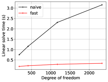
Figure 5: The total time of linear solves after the solver is run up to $t=3520$. The $x$-axis corresponds to the size of the solution (particle and channel). $M=N$ tested are $5,10,20$ and $30$. The time to assemble the coefficients of the linear systems (4.2) are not included, since they can be precomputed.

Figure 6 compares the total time of simulation between the naive solver and the fast solver for varied $M=N$. We especially observe that the time spent on evaluating the Jacobian is drastically reduced. At $M=30$, the fast solver outperforms the naive method by $\approx 5000$ times.

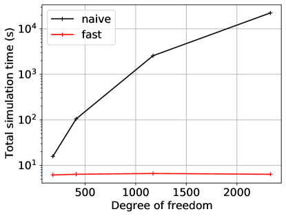
Figure 6: The total simulation time until full discharge at $1$C. $M=N$ tested are $5,10,20$ and $30$.

The code used to generate the performance measurements can be found in the script performance/full_simulation_comparison.py. The data in Table 6 was also generated by the same code. The script performance/reordered_performance.py was used to obtain data for Table 7 and Table 5.

5.3 Comparison between the fast solver and other solvers

We also compare the solver against LIONSIMBA [15], DUALFOIL [7] and COMSOL [14]. We take the P2D model simulation data of LIONSIMBA, DUALFOIL and COMSOL from [15], which simulates a discharge cycle of 1C under isothermal conditions, done on a Windows 7 PC with 8GB of RAM. We also include the runtimes of LIONSIMBA obtained on our machine (3.5 GHz Dual-Core Intel Core i7 with 8GB of RAM). For these simulations, the grid size was kept the same across all battery sections. Table 5 shows that the simulation times from our fast solver stay roughly constant for the resolutions tested, whereas this is not true for other solvers.

$M$	10	20	30	40	50
Fast solver†	4.09 s	4.24 s	3.98 s	4.15 s	4.49 s
LIONSIMBA†	7.46 s	9.85 s	15.48 s	26.80 s	54.60 s
LIONSIMBA*	28 s	57 s	105 s	134 s	223 s
DUALFOIL*	28 s	69 s	97 s	137 s	185 s
COMSOL*	96 s	114 s	143 s	189 s	244 s

Table 5: Comparison of simulation time between solvers. ^†The data was obtained from 3.5 GHz Dual-Core Intel Core i7 with 8GB of RAM. *The data was taken from [15] collected on a different machine.

6 Results

The fast method improves the efficiency of the naive solver in two ways. Firstly, by decoupling the system, we reduce the time to solve the linear systems, as shown in Figure 5. The figure compares performance between the general sparse linear solver and the banded solver (scipy.linalg.solve_banded) along with tridiagonal solves with $LU$ factorisation. By reformulating the problem and taking advantage of the linear structure in (4.2), we improve the linear algebraic efficiency.

Secondly, we work around the major bottleneck of the computation by implementing our own Jacobian building function. Under the AD framework with JAX, a large portion of the simulation time is spent on evaluating the Jacobian and $\bm{F}(U)$. This dominates the total simulation time shown in Figure 6. JAX’s Jacobian function takes up to six hours to evaluate the Jacobians with the full channel and particle system. Decoupling alone without using our custom Jacobian building function (the decoupled method) significantly cuts the time to evaluate the Jacobian. Evaluating the Jacobian of size $\mathcal{O}(M)\times\mathcal{O}(M)$ is much cheaper with JAX’s Jacobian function, as opposed to $\mathcal{O}(NM)\times\mathcal{O}(NM)$. For all grid points tested, the decoupled method is faster than the naive method, drastically outperforming as $M$ increases. The decoupled formulation achieves performance that is $\approx 870$ times faster than the naïve method at $M=30$.

The fast method further improves the efficiency. JAX is only used to compute the partial derivatives via backward mode differentiation. Compared to the decoupled method, the custom function reduces the time to evaluate the Jacobian up to $\approx 7$ times at $M=30$. This is evidently due to the fact that the banded matrix in diagonal ordered form (of size $47\times N_{tot}$) has a fixed number of rows and only the number of columns increases with $M_{a},M_{p},M_{s},M_{n}$ and $M_{z}$. Table 6 compares the time to auto differentiate and evaluate $\mathcal{J}(U)$ and $\bm{F}(U)$ and the total simulation time of the three methods discussed.

	Evaluation (s)	Total (s)
Naive	$2.22\text{\times}{10}^{4}$ s	$2.31\text{\times}{10}^{4}$ s
Decoupled only (decoupled method)	15.72 s	21.63 s
Decoupled & Banded (fast method)	0.3943 s	3.898 s

Table 6: Evaluation time is the time spent on evaluating $\mathcal{J}(U)$ and $\bm{F}(U)$. The simulations were compared at $M=30$.

Table 7 summarises the performance of the fast solver. There is an initial overhead ($\approx 15$ seconds) that comes with using XLA compiler, which can be precomputed before the actual simulation. Therefore, we do not factor it into the total time. We observe that the total time spent on the simulation stays roughly constant between three to five seconds. The grids at all battery domains were set equal, with $N_{p}=N_{n}=10,20,30,40,50$ and $M_{a}=M_{p}=M_{s}=M_{n}=M_{z}=10,20,30,40,50$. For these grid resolutions, we observe that the evaluation and solve times are not the dominating factors but the miscellaneous calculation overhead. This explains why the simulation time seem constant with respect to $N$ and $M$. Choosing $M=N\gtrapprox 100$, a clearer upward trend emerges where the solve time dominates the computation (results not included). For practical applications, such fine resolution may not be needed and $M=N\leq 50$ would suffice.

$M$	10	20	30	40	50
Solve	0.213	0.289	0.346	0.4174	0.532
Evaluation	0.376	0.412	0.386	0.426	0.483
Total	4.092	4.243	3.987	4.1536	4.494

Table 7: Averaged times of the fast solver over 20 runs. Solve time indicates the total time spent on linear solves. Evaluation time is the time spent on evaluating $\mathcal{J}(U)$ and $\bm{F}(U)$.

7 Conclusion

We have implemented a fast and robust implementation of the full P2D model without reducing the model. We give a thorough description of the discretisation of the PDAE involving cell-centred finite differences and backward Euler time stepping. The resulting system is a set of nonlinear equations, which can be solved by Newton’s method.

In order to robustly compute the Jacobian at every Newton’s iteration, automatic differentiation is used via the Python package JAX. Because the full P2D model has a linear structure in the particle equations (2.1), we are able to decouple the particle and channel equations at each time step. After decoupling, we solve one large tridiagonal linear system per time step and smaller sparse systems (channel equations) within the Newton iterations. The full system is thus solved more efficiently.

The decoupled method enables us to run the simulation 1C discharge cycle in a reasonable time under the AD framework, whereas such framework is infeasible when we use the naive method. This was made possible by rearranging the variables in the channel equations to create a matrix that is banded, which can be solved efficiently. The computation was made more efficient by directly building the banded Jacobian using the XLA compiler.

An additional way we can increase the efficiency is implementing a adaptive time stepping scheme, based on error on $\bm{c}$ only. We have implemented this for the scaled P2D model based on [27], which is a work in progress by Hennessey et al. The adaptive time stepping takes larger time steps in the beginning and gradually adjusts to smaller steps as the problem gets harder near the end of the cycle. For the scaled P2D model, it improved the efficiency by roughly a factor of two compared to the fixed time stepping scheme. This is future work to be explored.

We have demonstrated that by exploiting the structure of the problem, and utilizing state-of-art software, the complex P2D model can be solved accurately in under a few seconds. The fast solver can be potentially used as part of larger computations, such as optimizing multiple-battery pack behaviours. The solver would be especially useful where the P2D model has to be solved repeatedly over many cycles for estimation, optimization or control purposes.

Appendix A Symbols and Additional equations

[title=List of Symbols,type=symbols,style=long]

Open Circuit Potential

$\bm{U}_{p}=\bm{U}_{\text{p,ref}}+(T(x,t)-T_{\text{ref}})\frac{\partial\bm{U}_{p}}{\partial\bm{T}}\rvert_{T_{\text{ref}}}$

$\bm{U}_{n}=\bm{U}_{\text{n,ref}}+(T(x,t)-T_{\text{ref}})\frac{\partial\bm{U}_{n}}{\partial\bm{T}}\rvert_{T_{\text{ref}}}$

Entropy Change

$\frac{\partial\bm{U}_{p}}{\partial\bm{T}}\rvert_{T_{\text{ref}}}=-0.001\left(\frac{0.199521039-0.928373822\theta_{p}+1.364550689000003\theta_{p}^{2}-0.6115448939999998\theta_{p}^{3}}{1-5.661479886999997\theta_{p}+11.47636191\theta_{p}^{2}-9.82431213599998\theta_{p}^{3}+\ 3.046755063\theta_{p}^{4}}\right)$

$\frac{\partial\bm{U}_{n}}{\partial\bm{T}}\rvert_{T_{\text{ref}}}=0.001\left(\frac{\begin{multlined}0.005269056+3.299265709\theta_{n}-91.79325798\theta_{n}^{2}+1004.911008\theta_{n}^{3}-5812.278127\theta_{n}^{4}\\ +19329.7549\theta_{n}^{5}-37147.8947\theta_{n}^{6}+38379.18127\theta_{n}^{7}-16515.05308\theta_{n}^{8}\end{multlined}0.005269056+3.299265709\theta_{n}-91.79325798\theta_{n}^{2}+1004.911008\theta_{n}^{3}-5812.278127\theta_{n}^{4}\\ +19329.7549\theta_{n}^{5}-37147.8947\theta_{n}^{6}+38379.18127\theta_{n}^{7}-16515.05308\theta_{n}^{8}}{\begin{multlined}1-48.09287227\theta_{n}+1017.234804\theta_{n}^{2}-10481.80419\theta_{n}^{3}+59431.3\theta_{n}^{4}\\ -195881.6488\theta_{n}^{5}+374577.3152\theta_{n}^{6}-385821.1607\theta_{n}^{7}+165705.8597\theta_{n}^{8}\end{multlined}1-48.09287227\theta_{n}+1017.234804\theta_{n}^{2}-10481.80419\theta_{n}^{3}+59431.3\theta_{n}^{4}\\ -195881.6488\theta_{n}^{5}+374577.3152\theta_{n}^{6}-385821.1607\theta_{n}^{7}+165705.8597\theta_{n}^{8}}\right)$

$\theta_{p}=\frac{c^{*}_{s,p}(x,t)}{c^{\text{max}}_{s,p}}$

$\theta_{n}=\frac{c^{*}_{s,n}(x,t)}{c^{\text{max}}_{n,p}}$

Open circuit potential

$U_{\text{p,ref}}=\frac{-4.656+88.669\theta_{p}^{2}-401.119\theta_{p}^{4}+342.909\theta_{p}^{6}-462.471\theta_{p}^{8}+433.434\theta_{p}^{1}0}{-1+18.933\theta_{p}^{2}-79.532\theta_{p}^{4}+37.311\theta_{p}^{6}-73.083\theta_{p}^{8}+95.96\theta_{p}^{1}0}$

$U_{\text{n,ref}}=0.7222+0.1387\theta_{n}+0.029\theta_{n}^{0.5}-\frac{0.0172}{\theta_{n}}+\frac{0.0019}{\theta^{1.5}}+0.2808e^{0.9-15\theta_{n}}-0.7984e^{0.4465\theta_{n}-0.4108}$

Heat source terms (electrodes)

$\bm{Q}_{\text{ohm}}=\sigma_{\text{eff},i}\left(\frac{\partial\Psi(x,t)}{\partial x}\right)^{2}+\kappa_{\text{eff},i}\left(\frac{\partial\Phi_{e}(x,t)}{\partial x}\right)^{2}+\frac{2\kappa_{\text{eff},i}RT(x,t)}{F}(1-t_{+})\frac{\partial\ln u(x,t)}{\partial x}\frac{\Phi_{e}(x,t)}{\partial x}$

$\bm{Q}_{\text{rxn}}=Fa_{i}j(x,t)\eta_{i}(x,t)$

$\bm{Q}_{\text{rev}}=Fa_{i}j(x,t)T(x,t)\frac{\partial U_{i}}{\partial T}\rvert_{T_{\text{ref}}}$

Heat source terms (separator)

$\bm{Q}_{\text{ohm}}=\kappa_{\text{eff},i}\left(\frac{\partial\Phi_{e}(x,t)}{\partial x}\right)^{2}+\frac{2\kappa_{\text{eff},i}RT(x,t)}{F}(1-t_{+})\frac{\partial\ln u(x,t)}{\partial x}\frac{\Phi_{e}(x,t)}{\partial x}$

Coefficients

$\bm{D}_{\text{eff},i}=\epsilon_{i}^{\text{brugg}_{i}}\times 10^{-4}\times 10^{-4.43-\frac{54}{T(x,t)-229-5\times 10^{-3}u(x,t)}-0.22\times 10^{-3}u(x,t)}$

$\begin{aligned} \kappa_{\text{eff},i}=\epsilon_{i}^{\text{brugg}_{i}}\times 10^{-4}\times u(x,t)\left(-10.5+0.668\times 10^{-3}u(x,t)+0.494\times 10^{-6}u(x,t)^{2}+\right.\\ \left.T(x,t)(0.074-1.78\times 10^{-5}u(x,t)-8.86\times 10^{-10}u(x,t)^{2})+\right.\\ \left.T(x,t)^{2}(-6.96\times 10^{-5}+2.8\times 10^{-8}u(x,t))\right)^{2}\end{aligned}$

$k_{\text{eff}}=k_{i}e^{\frac{E^{k_{i}}_{a}}{R}\left(\frac{1}{T(x,t)}-\frac{1}{T_{\text{ref}}}\right)}$

$D^{s}_{\text{eff},i}=D^{s}_{i}e^{\frac{E^{D^{s}_{i}}_{a}}{R}\left(\frac{1}{T(x,t)}-\frac{1}{T_{\text{ref}}}\right)}$

$\sigma_{\text{eff},i}=\sigma_{i}(1-\epsilon_{i}-\epsilon_{f,i})$

$\Upsilon=\frac{2(1-t_{+})R}{F}$

Appendix B Parameters used in simulation

		Al CC	Cathode	Separator	Anode	Carbon CC
$c_{e}^{\text{init}}$	[mol/m3]	-	1000	1000	1000	-
$c_{s}^{\text{avg, init}}$	[mol/m3]	-	25751	-	26128	-
$c_{s}^{\text{max}}$	[mol/m3]	-	51554	-	30555	-
$D_{i}$	[m${}^{2}/s$]	-	$7.5\times 10^{-10}$	$7.5\times 10^{-10}$	$7.5\times 10^{-10}$	-
$D^{s}_{i}$	[m${}^{2}/s$]	-	$10^{-14}$	-	$3.9\times 10^{-14}$	-
$k_{i}$	[m${}^{2.5}/$ (mol0.5s)]	-	$2.334\times 10^{-11}$	-	$5.301\times 10^{-11}$	-
$l_{i}$	[m]	$10^{-5}$	$8\times 10^{-5}$	$2.5\times 10^{-5}$	$8.8\times 10^{-5}$	$10^{-5}$
$R_{p,i}$	[m]	-	$2\times 10^{-6}$	-	$2\times 10^{-6}$	-
$\rho_{i}$	[kg/m3]	2700	2500	1100	2500	8940
$C_{p,i}$	[J/(kg K)]	897	700	700	700	385
$\lambda_{i}$	[W/(m K)]	237	2.1	0.16	1.7	401
$\sigma_{i}$	[S/m]	$3.55\times 10^{7}$	100	-	100	$5.96\times 10^{7}$
$\epsilon_{i}$	-	-	0.385	0.724	0.485	-
$a_{i}$	[m2/m3]	-	885000	-	723600	-
$E^{D^{s}_{i}}_{a}$	[J/mol]	-	5000	-	5000	-
$E^{k_{i}}_{a}$	[J/mol]	-	5000	-	5000	-
brugg	-	-	4	4	4	-
$F$	96485 [C/mol]	-	-	-	-	-
$R$	8.314472 [J/(mol K)]	-	-	-	-	-
$t_{+}$	0.354
$\epsilon_{f,i}$	-	-	0.025	-	0.0326	-

References

-
[1]
N. Nitta, F. Wu, J. T. Lee, G. Yushin,
Li-ion
battery materials: present and future, Materials Today 18 (5) (2015) 252 –
264.
doi:https://doi.org/10.1016/j.mattod.2014.10.040.
URL http://www.sciencedirect.com/science/article/pii/S1369702114004118 - [2] J. Heelan, E. Gratz, Z. Zheng, Q. Wang, M. Chen, D. Apelian, Y. Wang, Current and prospective li-ion battery recycling and recovery processes, The Journal of The Minerals, Metals & Materials Society (TMS) 68 (10) (2016) 2632–2638.
- [3] B. Pattipati, K. Pattipati, J. P. Christopherson, S. M. Namburu, D. V. Prokhorov, Liu Qiao, Automotive battery management systems, in: 2008 IEEE AUTOTESTCON, 2008, pp. 581–586.
- [4] K. Liu, K. Li, J. Deng, A novel hybrid data-driven method for li-ion battery internal temperature estimation, in: 2016 UKACC 11th International Conference on Control (CONTROL), IEEE, 2016, pp. 1–6.
-
[5]
K. A. Severson, P. M. Attia, N. Jin, N. Perkins, B. Jiang, Z. Yang, M. H. Chen,
M. Aykol, P. K. Herring, D. Fraggedakis, M. Z. Bazant, S. J. Harris, W. C.
Chueh, R. D. Braatz,
Data-driven prediction of
battery cycle life before capacity degradation, Nature Energy 4 (5) (2019)
383–391.
doi:10.1038/s41560-019-0356-8.
URL https://doi.org/10.1038/s41560-019-0356-8 -
[6]
M.-F. Ng, J. Zhao, Q. Yan, G. J. Conduit, Z. W. Seh,
Predicting the state of
charge and health of batteries using data-driven machine learning, Nature
Machine Intelligence 2 (3) (2020) 161–170.
doi:10.1038/s42256-020-0156-7.
URL https://doi.org/10.1038/s42256-020-0156-7 - [7] M. Doyle, Modeling of galvanostatic charge and discharge of the lithium/polymer/insertion cell, Journal of The Electrochemical Society 140 (6) (1993) 1526. doi:10.1149/1.2221597.
- [8] M. Guo, G. Sikha, R. E. White, Single-particle model for a lithium-ion cell: Thermal behavior, Journal of The Electrochemical Society 158 (2) (2010) A122.
- [9] E. Prada, D. Di Domenico, Y. Creff, J. Bernard, V. Sauvant-Moynot, F. Huet, Simplified electrochemical and thermal model of LiFePO4-graphite Li-ion batteries for fast charge applications, Journal of The Electrochemical Society 159 (9) (2012) A1508.
- [10] V. Ramadesigan, V. Boovaragavan, J. C. Pirkle Jr, V. R. Subramanian, Efficient reformulation of solid-phase diffusion in physics-based lithium-ion battery models, Journal of The Electrochemical Society 157 (7) (2010) A854.
- [11] X. Han, M. Ouyang, L. Lu, J. Li, Simplification of physics-based electrochemical model for lithium ion battery on electric vehicle. Part I: Diffusion simplification and single particle model, Journal of Power Sources 278 (2015) 802–813.
- [12] A. Jokar, B. Rajabloo, M. Désilets, M. Lacroix, Review of simplified pseudo-two-dimensional models of lithium-ion batteries, Journal of Power Sources 327 (2016) 44–55.
-
[13]
V. Ramadesigan, P. W. C. Northrop, S. De, S. Santhanagopalan, R. D. Braatz,
V. R. Subramanian, Modeling and
simulation of lithium-ion batteries from a systems engineering perspective,
Journal of The Electrochemical Society 159 (3) (2012) R31–R45.
doi:10.1149/2.018203jes.
URL https://doi.org/10.1149%2F2.018203jes -
[14]
L. Cai, R. E. White,
Mathematical
modeling of a lithium ion battery with thermal effects in COMSOL Inc.
Multiphysics (MP) software, Journal of Power Sources 196 (14) (2011) 5985
– 5989.
doi:https://doi.org/10.1016/j.jpowsour.2011.03.017.
URL http://www.sciencedirect.com/science/article/pii/S0378775311005994 - [15] M. Torchio, L. Magni, R. B. Gopaluni, R. D. Braatz, D. M. Raimondo, LIONSIMBA: a Matlab framework based on a finite volume model suitable for Li-ion battery design, simulation, and control, Journal of The Electrochemical Society 163 (7) (2016) A1192.
- [16] G. G. Botte, V. R. Subramanian, R. E. White, Mathematical modeling of secondary lithium batteries, Electrochimica Acta 45 (15-16) (2000) 2595–2609.
- [17] L. R. Petzold, Description of DASSL: a differential/algebraic system solver, Tech. rep., Sandia National Labs., Livermore, CA (USA) (1982).
- [18] A. C. Hindmarsh, P. N. Brown, K. E. Grant, S. L. Lee, R. Serban, D. E. Shumaker, C. S. Woodward, Sundials: Suite of nonlinear and differential/algebraic equation solvers, ACM Transactions on Mathematical Software (TOMS) 31 (3) (2005) 363–396.
-
[19]
J. Bradbury, R. Frostig, P. Hawkins, M. J. Johnson, C. Leary, D. Maclaurin,
S. Wanderman-Milne, JAX: composable
transformations of Python+NumPy programs (2018).
URL http://github.com/google/jax - [20] V. D. Bruggeman, Berechnung verschiedener physikalischer Konstanten von heterogenen Substanzen. I. Dielektrizitätskonstanten und Leitfähigkeiten der Mischkörper aus isotropen Substanzen, Annalen der physik 416 (7) (1935) 636–664.
-
[21]
J. Newman, K. Thomas-Alyea,
Electrochemical
Systems, The ECS Series of Texts and Monographs, Wiley, 2004.
URL https://books.google.ca/books?id=vArZu0HM-xYC -
[22]
U. Ascher, L. Petzold,
Computer Methods for
Ordinary Differential Equations and Differential-Algebraic Equations, Other
Titles in Applied Mathematics, Society for Industrial and Applied
Mathematics, 1998.
URL https://books.google.ca/books?id=VL51G5JYYAYC - [23] J. W. Thomas, Numerical Partial Differential Equations: Finite Difference Methods, Vol. 22 of Texts in Applied Mathematics, Springer-Verlag, New York, 1995.
- [24] R. L. Burden, J. D. Faires, Numerical analysis (2011).
- [25] A. G. Baydin, B. A. Pearlmutter, A. A. Radul, J. M. Siskind, Automatic differentiation in machine learning: a survey, The Journal of Machine Learning Research 18 (1) (2017) 5595–5637.
-
[26]
X. team within Google, XLA: Optimizing
compiler for machine learning.
URL https://www.tensorflow.org/xla - [27] M. Hennesy, I. Moyles, T. Myers, B. Wetton, The P2D model for Li-ion battery electrodes: When is it really needed?