The Principle of equal Probabilities of Quantum States

Abstract

The statistical problem of the distribution of $s$ quanta of equal energy $\epsilon_{0}$ and total energy $E$ among $N$ distinguishable particles is resolved using the conventional theory based on Boltzmann’s principle of equal probabilities of configurations of particles distributed among energy levels and the concept of average state. In particular, the probability that a particle is in the $\kappa$-th energy level i.e. contains $\kappa$ quanta, is given by

$$p(\kappa)=\displaystyle\frac{\displaystyle\binom{N+s-\kappa-2}{N-2}}{\displaystyle\binom{N+s-1}{N-1}}\;\;\;;\;\;\;\kappa=0,1,2,\cdots,s$$

In this context, the special case ($N=4$, $s=4$) presented indicates that the alternative concept of most probable state is not valid for finite values of $s$ and $N$.
In the present article we derive alternatively $p(\kappa)$ by distributing $s$ quanta over $N$ particles and by introducing a new principle of equal probability of quantum states, where the quanta are indistinguishable in agreement with the Bose statistics. Therefore, the analysis of the two approaches presented in this paper highlights the equivalence of quantum theory with classical statistical mechanics for the present system.
At the limit $\epsilon_{o}\rightarrow 0$; $s\rightarrow\infty$; $s\epsilon_{o}=E\sim$ fixed, where the energy of the particles becomes continuous, $p(\kappa)$ transforms to the Boltzmann law

$$P(\epsilon)=\displaystyle\frac{1}{\langle\epsilon\rangle}e^{-{\frac{\epsilon}{\langle\epsilon\rangle}}}\;\;\;;\;\;\;0\leq\epsilon<+\infty$$

where $\langle\epsilon\rangle=E/N$. Hence, the classical principle of equal a priori probabilities for the energy of the particles leading to the above law, is justified here by quantum mechanics.

1 Introduction

Consider a system of $N$ distinguishable particles having total energy $E$. If the energy is quantised in equal parts: $E=s\epsilon_{o}$, where $s$ is the total number of quanta, the particles will occupy the discrete energy levels $0,\epsilon_{o},2\epsilon_{o},\cdots,s\epsilon_{o}$ (briefly $0,1,2,\cdots,s$). In the present article we consider the Boltzmann principle [Boltzmann] of equal probabilities of configurations (complexions) for particles distributed among energy levels according to the equations:

$$n_{0}+n_{1}+n_{2}+\cdots+n_{s}=N$$ (1)

$$n_{1}+2n_{2}+3n_{3}+\cdots+sn_{s}=s$$ (2)

where $n_{0}\geq 0,n_{1}\geq 0,n_{2}\geq 0,\cdots,n_{s}\geq 0$ are the respective number of particles occupying the $s+1$ energy levels. As it is well known, each group $(n_{0},n_{1},n_{2},\cdots,n_{s})$ which is a solution of Eqs (1, 2) defines in this case a state of the system. The total number of states $S_{I}$ created by Eqs (1, 2) can be obtained considering the $s$ dimensional space $[n_{1},n_{2},\cdots,n_{s}]$. In this space Eq.(1) defines a family of hyperplanes $n_{1}+n_{2}+\cdots+n_{s}=N-n_{0}$ where the number $n_{0}$ of particles having zero energy is a parameter $n_{0}=0,1,2,\cdots,N$ and where each hyperplane of this family cuts symmetrically all axes of the $s$ dimensional space at $N-n_{0}$. The total number of non-negative integer solutions of Eq.(1) is given by the Bose formula [Ladau]:

$${B}(N,s+1)=\sum_{n_{0}=0}^{N}\frac{(N-n_{0}+s-1)!}{(N-n_{0})!(s-1)!}=\begin{pmatrix}N+s\\ s\end{pmatrix}$$ (3)

On the other hand, Eq.(2) defines in the $s$ dimensional space $[n_{1},n_{2},\cdots,n_{s}]$ a single nonsymmetric hyperplane cutting the axis $n_{1}$ at $n_{1}=s$, the axis $n_{2}$ at $n_{2}=\frac{s}{2}$, $\cdots$, the axis $n_{s}$ at $n_{s}=1$. In this case the number of non-negative integer solutions of Eq.(2) is equal to the number $p_{s}$ of partitions of the number $s$. According to previous work (M. Psimopoulos, ‘Reduced Harmonic Representation of Partitions’, 2011):

$$p_{s}=\frac{2}{\pi}\int_{0}^{\frac{\pi}{2}}\prod_{\kappa=1}^{s}\frac{sin((s+\kappa)x)}{sin(\kappa x)}cos[({s^{2}}-2s)x]\;dx$$ (4)

Considering next both Eqs (1, 2) we have two cases:
If $N\geq s$ the family of hyperplanes defined by Eq.(1) fully covers the energy hyperplane defined by Eq.(2) so that the total number of states ${S}_{I}$ corresponding to the joint solution of Eqs (1, 2) is

$${S}_{I}=p_{s}$$ (5)

If $N<s$ the family of hyperplanes defined by Eq.(1) does not fully cover the energy hyperplane defined by Eq.(2) so that the total number of states ${S}_{I}$ corresponding to the joint solution of Eqs (1, 2) obeys

$${S}_{I}<p_{s}$$ (6)

In this case no close formula for the number of states ${S}_{I}$ has been obtained. However, it must be stressed that since the particles are distinguishable, it is not the number of states, but the number of configurations that forms the statistical basis of the present system. In particular, there are

$${C}(n_{0},n_{1},n_{2},\cdots,n_{s})=\frac{N!}{n_{0}!n_{1}!n_{2}!\cdots n_{s}!}$$ (7)

configurations corresponding to each state $(n_{0},n_{1},n_{2},\cdots,n_{s})$.

According to Boltzmann’s principle: The probability that a state will occur is given by

$$p(n_{0},n_{1},n_{2},\cdots,n_{s})=\frac{1}{{C}_{I}}{C}(n_{0},n_{1},n_{2},\cdots,n_{s})$$ (8)

where ${{C}_{I}}$ is the total number of configurations. On this basis, we derive explicitly in Section 2 the probability $p(\kappa)$ that a particle is in the $\kappa$-th energy level i.e contains $\kappa$ quanta. This part of the calculation is developed according to the concept of the average state [DarwinFowler] describing the system and it will be shown by considering the special case ($N=4$; $s=4$) that the alternative concept of most probable state used in the literature [Boltzmann] is not valid for finite values of $s$ and $N$.

Next, we prove that the above conventional theory gives results that are identical to the ones obtained by considering the distribution of quanta among particles according to the equation

$$\kappa_{1}+\kappa_{2}+\kappa_{3}+\cdots+\kappa_{N}=s$$ (9)

where $\kappa_{1}\geq 0,\kappa_{2}\geq 0,\kappa_{3}\geq 0,\cdots,\kappa_{N}\geq 0$ are the respective numbers of quanta attributed to the $N$ particles, defining a state ($\kappa_{1},\kappa_{2},\cdots,\kappa_{N}$) of the system. However, it is demonstrated in Section 3 that this identity of results is valid only if the quanta obey a principle of equal probabilities of states rather than configurations, which leads to the conclusion that the quanta are indistinguishable and that the Bose statistics [Ladau] is valid. As it is well know from the simple problem of distributing $s$ balls into $N$ boxes, the number of states (or solutions of Eq.(9)) is given by

$${S}_{II}=\frac{(N+s-1)!}{s!(N-1)!}$$ (10)

Note that Eq.(10) will be proved rigorously in Section 3.

The mathematical method used throughout the article is the Darwin-Fowler technique of generating functions [DarwinFowler][terHaar] that are appropriate for the study of both approaches.

In the final part of the paper we discuss the passage to the classical limit $\epsilon_{o}\rightarrow 0$; $s\rightarrow\infty$; $s\epsilon_{o}=E$ where the particles have continuous energies. In this case the principle of equal probabilities of quantum states introduced through Eq.(9) transforms to the principle of equal a priori probabilities of classical statistical mechanics, justifying the latter principle as a limiting hypothesis based on quantum mechanics.

Simple Example

Before developing the general theory, let us present a simple example in order to explain the main idea of the paper. Consider a system of $N=4$ distinguishable particles containing $s=4$ quanta of equal energy.
I. According to the Boltzmann method[Boltzmann], the statistical analysis of this system is based on Eqs (1, 2) which in the present case have the form:

$$n_{0}+n_{1}+n_{2}+n_{3}+n_{4}=4$$ (11)

$$n_{1}+2n_{2}+3n_{3}+4n_{4}=4$$ (12)

where $n_{0},n_{1},n_{2},n_{3},n_{4}$ represent the number of particles occupying the energy levels $\kappa=0,1,2,3,4$ respectively. We observe that there are $S_{I}=5$ states of this system (equal to the number of non-negative solutions of Eqs (11, 12)) given in Table 1.

$n_{0}$	$n_{1}$	$n_{2}$	$n_{3}$	$n_{4}$
0	4	0	0	0
1	2	1	0	0
2	0	2	0	0
2	1	0	1	0
3	0	0	0	1

Table 1: The 5 states of the system $N=4$; $s=4$.

Explicitly, according to Eqs (4, 5) the number of states is equal to the number of partitions $p_{4}$ of number $4$:

$${S}_{I}=p_{4}=\frac{2}{\pi}\int_{0}^{\frac{\pi}{2}}\frac{sin(5x)sin(6x)sin(7x)sin(8x)}{sin(x)sin(2x)sin(3x)sin(4x)}cos(8x)\;dx=5$$ (13)

From Eq.(7) the number of configurations for each state of Table 1 reads:

$$\begin{split}{C}(0,4,0,0,0)=\frac{4!}{0!4!0!0!0!}=1\\ {C}(1,2,1,0,0)=\frac{4!}{1!2!1!0!0!}=12\\ {C}(2,0,2,0,0)=\frac{4!}{2!0!2!0!0!}=6\\ {C}(2,1,0,1,0)=\frac{4!}{2!1!0!1!0!}=12\\ {C}(3,0,0,0,1)=\frac{4!}{3!0!0!0!1!}=4\end{split}$$ (14)

and the total number of configurations is:

$${C}_{I}=1+12+6+12+4=35$$ (15)

According to the Boltzmann principle, all configurations have equal probability of occurrence. Therefore from Eq.(8), the corresponding probabilities of the five states of Table 1 are given by: rCl p(0, 4, 0, 0, 0) & = 135 ;  p(1, 2, 1, 0, 0)= 1235 ;  p(2, 0, 2, 0, 0)=635

p(2, 1, 0, 1, 0) = 1235 ;  p(3, 0, 0, 0, 1) = 435

Next, we define $p(n/\kappa)$ to be the conditional probability that there are $n$ particles in the $\kappa$-th energy level. We calculate $p(n/\kappa)$ for each particular level $\kappa=0,1,2,3,4$ using the probabilities of Eqs (15) as follows:

Energy level $\kappa=0$:

$$p(0/0)=\frac{1}{35}\;;\;\;p(1/0)=\frac{12}{35}\;;\;\;p(2/0)=\frac{6}{35}+\frac{12}{35}=\frac{18}{35}\;;\;\;p(3/0)=\frac{4}{35}\;;\;\;p(4/0)=0$$ (16)

Normalisation: $p(0/0)+p(1/0)+p(2/0)+p(3/0)+p(4/0)=1$.
Average number of particles in level $\kappa=0$:

$$\langle n_{0}\rangle=0\cdot p(0/0)+1\cdot p(1/0)+2\cdot p(2/0)+3\cdot p(3/0)+4\cdot p(4/0)=\frac{60}{35}$$ (17)

Energy level $\kappa=1$:

$$p(0/1)=\frac{6}{35}+\frac{4}{35}=\frac{10}{35}\;;\;\;p(1/1)=\frac{12}{35}\;;\;\;p(2/1)=\frac{12}{35}\;;\;\;p(3/1)=0\;;\;\;p(4/1)=\frac{1}{35}$$ (18)

Normalisation: $p(0/1)+p(1/1)+p(2/1)+p(3/1)+p(4/1)=1$.
Average number of particles in level $\kappa=1$:

$$\langle n_{1}\rangle=0\cdot p(0/1)+1\cdot p(1/1)+2\cdot p(2/1)+3\cdot p(3/1)+4\cdot p(4/1)=\frac{40}{35}$$ (19)

Energy level $\kappa=2$:

$$p(0/2)=\frac{1}{35}+\frac{12}{35}+\frac{4}{35}=\frac{17}{35}\;;\;\;p(1/2)=\frac{12}{35}\;;\;\;p(2/2)=\frac{6}{35}\;;\;\;p(3/2)=0\;;\;\;p(4/2)=0$$ (20)

Normalisation: $p(0/2)+p(1/2)+p(2/2)+p(3/2)+p(4/2)=1$.
Average number of particles in level $\kappa=2$:

$$\langle n_{2}\rangle=0\cdot p(0/2)+1\cdot p(1/2)+2\cdot p(2/2)+3\cdot p(3/2)+4\cdot p(4/2)=\frac{24}{35}$$ (21)

Energy level $\kappa=3$:

$$p(0/3)=\frac{1}{35}+\frac{12}{35}+\frac{6}{35}+\frac{4}{35}=\frac{23}{35}\;;\;\;p(1/3)=\frac{12}{35}\;;\;\;p(2/3)=0\;;\;\;p(3/3)=0\;;\;\;p(4/3)=0$$ (22)

Normalisation: $p(0/3)+p(1/3)+p(2/3)+p(3/3)+p(4/3)=1$.
Average number of particles in level $\kappa=3$:

$$\langle n_{3}\rangle=0\cdot p(0/3)+1\cdot p(1/3)+2\cdot p(2/3)+3\cdot p(3/3)+4\cdot p(4/3)=\frac{12}{35}$$ (23)

Energy level $\kappa=4$:

$$p(0/4)=\frac{1}{35}+\frac{12}{35}+\frac{6}{35}+\frac{12}{35}=\frac{31}{35}\;;\;\;p(1/4)=\frac{4}{35}\;;\;\;p(2/4)=0\;;\;\;p(3/4)=0\;;\;\;p(4/4)=0$$ (24)

Normalisation: $p(0/4)+p(1/4)+p(2/4)+p(3/4)+p(4/4)=1$.
Average number of particles in level $\kappa=4$:

$$\langle n_{4}\rangle=0\cdot p(0/4)+1\cdot p(1/4)+2\cdot p(2/4)+3\cdot p(3/4)+4\cdot p(4/4)=\frac{4}{35}$$ (25)

As expected

$$\langle n_{0}\rangle+\langle n_{1}\rangle+\langle n_{2}\rangle+\langle n_{3}\rangle+\langle n_{4}\rangle=\frac{60+40+24+12+4}{35}=4$$ (26)

From the above analysis we can define the average probability $p(\kappa)$ that a particle is in the $\kappa$-th energy level or equivalently that this particle contains $\kappa$ quanta of energy:

$$p(\kappa)=\frac{\langle n_{\kappa}\rangle}{N}\;\;\;;\;\;\;\kappa=0,1,2,\cdots,s$$ (27)

In the present case, according to the results of the Eqs (17-25), Eq.(27) gives for $p(\kappa)$ the values:

$$p(0)=\frac{15}{35}\;;\;\;p(1)=\frac{10}{35}\;;\;\;p(2)=\frac{6}{35}\;;\;\;p(3)=\frac{3}{35}\;;\;\;p(4)=\frac{1}{35}$$ (28)

represented in Figure 1.

Normalisation:

$$p(0)+p(1)+p(2)+p(3)+p(4)=1$$ (29)

The average number of quanta existing in a particle is:

$$\langle\kappa\rangle=1\cdot\frac{10}{35}+2\cdot\frac{6}{35}+3\cdot\frac{3}{35}+4\cdot\frac{1}{35}=1$$ (30)

which is consistent with $\langle\kappa\rangle=s/N$.

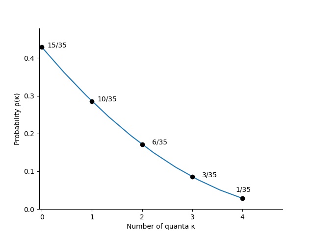
Figure 1: Example $N=4$; $s=4$: Graph of the probability that a particle is in the $\kappa$-th energy level.

We notice here that many authors, including Boltzmann [Boltzmann] define $p(\kappa)$ using the concept of most probable state instead of Eq.(27). According to this concept, one would derive the state (${n^{*}_{0}},{n^{*}_{1}},{n^{*}_{2}},\cdots,{n^{*}_{s}}$) that maximizes the number of configurations ${C}(n_{0},n_{1},\cdots,n_{s})$ given by Eq.(7) and he would define:

$$p(\kappa)=\frac{{n^{*}_{\kappa}}}{N}\;\;\;;\;\;\;\kappa=0,1,2,\cdots,s$$ (31)

We observe from the present example, however, that this is not a valid argument in general because the number of configurations ${C}(n_{0},n_{1},n_{2},n_{3},n_{4})$ given by Eqs (14) has two different maxima ${C}=12$ at (${n^{*}_{0}}=1,{n^{*}_{1}}=2,{n^{*}_{2}}=1,{n^{*}_{3}}=0,{n^{*}_{4}}=0$) and (${n^{*}_{0}}=2,{n^{*}_{1}}=1,{n^{*}_{2}}=0,{n^{*}_{3}}=1,{n^{*}_{4}}=0$). Therefore $p(\kappa)$ defined by Eq.(31) is not unique and the concept of most probable configuration cannot be used for finite $N$ and $s$. A rather general criticism of this approach can also be found in the paper of Darwin and Fowler [DarwinFowler].

II. Let us next distribute the energy quanta over the particles according to Eq.(9) which in the present case has the form:

$$\kappa_{1}+\kappa_{2}+\kappa_{3}+\kappa_{4}=4$$ (32)

where $\kappa_{1},\kappa_{2},\kappa_{3},\kappa_{4}$ are respectively the number of quanta contained in the particles $n=1,2,3,4$. According to Eq.(10), the total number of states (non-negative integer solutions of Eq.(32)) is

$$S_{II}=\frac{(4+4-1)!}{4!(4-1)!}=35$$ (33)

States $S_{II}$ (Eq.(33)) are represented by the points of the non-negative grid in 4-D space [$\kappa_{1},\kappa_{2},\kappa_{3},\kappa_{4}$] that also belong to the hyperplane defined by Eq.(32).

From Eqs (15, 33) we notice the very important equality ${C}_{I}=S_{II}$ which will be proved to be valid in general later in the paper.

Assuming that the states $S_{II}$ in Eq.(33) have equal probability of occurrence means that the quanta are indistinguishable and that the probability $p(\kappa)$ that any one of the four particles (say particle $1$) has $\kappa$ quanta, can be calculated by re-writing Eq.(32) in the form $\kappa_{2}+\kappa_{3}+\kappa_{4}=4-\kappa_{1}$ where $\kappa_{1}=0,1,2,3,4$.

$$\begin{split}\kappa_{1}=0:\;\;\kappa_{2}+\kappa_{3}+\kappa_{4}=4;\;\;S_{0}=\frac{(4+3-1)!}{4!(3-1)!}=\text{15 states};\;\;p(0)=\frac{S_{0}}{S_{II}}=\frac{15}{35}\\ \ \kappa_{1}=1:\;\;\kappa_{2}+\kappa_{3}+\kappa_{4}=3;\;\;S_{1}=\frac{(3+3-1)!}{3!(3-1)!}=\text{10 states};\;\;p(1)=\frac{S_{1}}{S_{II}}=\frac{10}{35}\\ \ \kappa_{1}=2:\;\;\kappa_{2}+\kappa_{3}+\kappa_{4}=2;\;\;S_{2}=\frac{(2+3-1)!}{2!(3-1)!}=\text{6 states};\;\;p(2)=\frac{S_{2}}{S_{II}}=\frac{6}{35}\\ \ \kappa_{1}=3:\;\;\kappa_{2}+\kappa_{3}+\kappa_{4}=1;\;\;S_{3}=\frac{(1+3-1)!}{1!(3-1)!}=\text{3 states};\;\;p(3)=\frac{S_{3}}{S_{II}}=\frac{3}{35}\\ \ \kappa_{1}=4:\;\;\kappa_{2}+\kappa_{3}+\kappa_{4}=0\;;\;\;S_{4}=\frac{(0+3-1)!}{0!(3-1)!}=\text{1 state}\;;\;\;p(4)=\frac{S_{4}}{S_{II}}=\frac{1}{35}\end{split}$$ (34)

We observe that results of Eqs (34) coincide with Eqs (28). This remarkable conclusion i.e. that $p(\kappa)$ can be obtained both by distributing distinguishable particles over energy levels or by distributing indistinguishable quanta over particles, will be proved to be valid in general in the next sections of the paper. An exact formula for $p(\kappa)$ will be derived for all finite values of $N$ and $s$ and the limit $N\rightarrow\infty$; $s\rightarrow\infty$; $s/N=\langle\kappa\rangle>>1$ will be studied.

2 Distribution of particles in energy levels

The total number of configurations of $N$ particles occupying the energy levels $\kappa=0,1,2,\cdots,s$ is given according to Eqs (1, 2) by

$${C}_{I}=\sum_{n_{0}=0}^{N}\sum_{n_{1}=0}^{N}\cdots\sum_{n_{s}=0}^{N}\frac{N!}{n_{0}!n_{1}!\cdots n_{s}!}\;\delta(n_{0}+n_{1}+n_{2}+\cdots+n_{s}-N)\;\delta(n_{1}+2n_{2}+\cdots+sn_{s}-s)$$ (35)

where

$$\delta(m-n)=\begin{cases}1&\text{; $m=n$}\\ 0&\text{; $m\neq n$}\\ \end{cases}$$ (36)

The generating function in this case is

$$f(x,y)=\sum_{n_{0}=0}^{\infty}\sum_{n_{1}=0}^{\infty}\cdots\sum_{n_{s}=0}^{\infty}\frac{N!}{n_{0}!n_{1}!\cdots n_{s}!}\;x^{n_{0}+n_{1}+\cdots+n_{s}}\;y^{n_{1}+2n_{2}+\cdots+sn_{s}}$$ (37)

where $0\leq x<1;\;\;0\leq y<1$. Taking separate factors in Eq.(37) we have

$$\sum_{n_{0}=0}^{\infty}\frac{x^{n_{0}}}{n_{0}!}=e^{x};\;\;\sum_{n_{1}=0}^{\infty}\frac{(xy)^{n_{1}}}{n_{1}!}=e^{xy};\;\;\sum_{n_{2}=0}^{\infty}\frac{(xy^{2})^{n_{2}}}{n_{2}!}=e^{x{y}^{2}};\;\;\cdots\;\;\sum_{n_{s}=0}^{\infty}\frac{(xy^{s})^{n_{s}}}{n_{s}!}=e^{x{y}^{s}}$$ (38)

and the generating function becomes

$$f(x,y)=N!\;e^{x}\cdot e^{xy}\cdot e^{x{y}^{2}}\cdots e^{x{y}^{s}}=N!\exp\big{\{}x(1+y+y^{2}+\cdots+y^{s})\big{\}}$$

so that

$$f(x,y)=N!\exp\Big{\{}x\Big{(}\frac{1-y^{s+1}}{1-y}\Big{)}\Big{\}}$$ (39)

Let us expand $f(x,y)$ in powers of $x$:

$$f(x,y)=N!\Big{\{}1+x\frac{1-y^{s+1}}{1-y}+\frac{x^{2}}{2!}\Big{(}\frac{1-y^{s+1}}{1-y}\Big{)}^{2}+\cdots\Big{\}}$$ (40)

the coefficient of $x^{N}$ in this expansion is

$$g(y)=\Big{(}\frac{1-y^{s+1}}{1-y}\Big{)}^{N}$$ (41)

We argue that if $g(y)$ is expressed in the form of a power series in $y$, then the coefficient of $y^{s}$ coincides with ${C}_{I}$ defined by Eq.(35):

$${C}_{I}=\frac{1}{s!}\Bigg{[}\frac{\partial^{s}}{\partial y^{s}}\Big{(}\frac{1-y^{s+1}}{1-y}\Big{)}^{N}\Bigg{]}_{y=0}$$ (42)

We observe that $(1-y^{s+1})^{N}\approx 1-Ny^{s+1}+\mathcal{O}[y^{2(s+1)}]$ and therefore rCl [ ∂s∂ys ( 1 - ys+11-y )^N ]_y = 0 & = [ ∂s∂ys 1(1-y)N ]_y = 0
= [ N(N+1)(N+2)⋯(N+s-1)(1-y)N+s ]_y=0 = (N+s-1)!(N-1)! and Eq.(42) gives the total number of configurations of all states:

$${C}_{I}=\frac{(N+s-1)!}{s!(N-1)!}$$ (43)

According to the Boltzmann principle, all configurations have equal probability of occurrence, therefore the probability that state $(n_{0},n_{1},n_{2},\cdots,n_{s})$ will occur is

$$p(n_{0},n_{1},n_{2},\cdots,n_{s})=\frac{1}{{C}_{I}}\frac{N!}{n_{0}!n_{1}!\cdots n_{s}!}\;\delta(n_{0}+n_{1}+\cdots+n_{s}-N)\;\delta(n_{1}+2n_{2}+\cdots+sn_{s}-s)$$ (44)

The average number of particles located in level $\kappa$ is rCl ⟨n_κ ⟩& = ∑_n_0=0^N∑_n_1=0^N ⋯∑_n_s=0^N n_κ   p(n_0, n_1, n_2, ⋯, n_s)
= N!CI ∑_n_0=0^N∑_n_1=0^N ⋯∑_n_s=0^N nκn0! n1! ⋯ns!   δ(n_0 + n_1+ ⋯+ n_s -N)   δ(n_1 + 2n_2 + ⋯+ s n_s -s) Generating function:

$$f_{\kappa}(x,y)=\frac{N!}{{C}_{I}}\sum_{n_{0}=0}^{\infty}\sum_{n_{1}=0}^{\infty}\cdots\sum_{n_{s}=0}^{\infty}\frac{n_{\kappa}}{n_{0}!n_{1}!\cdots n_{s}!}\;x^{n_{0}+n_{1}+\cdots+n_{s}}\;y^{n_{1}+2n_{2}+\cdots+sn_{s}}$$ (45)

where $0\leq x<1;\;\;0\leq y<1$. Taking separate factors we have rCl ∑_n_i=0^∞ & (x yi)nini! = e^x y^i    ;    i=0, 1, 2,⋯, κ-1, κ+1, ⋯, s
∑_n_κ=0^∞ n_κ (xyκ)nκnκ! = xy^κ ∑_n_κ=1^∞ (xyκ)nκ-1(nκ-1)! = xy^κ e^xy^κ so that rCl f_κ(x, y) & = N!CI xy^κ exp{ x (1+y+y^2+⋯+ y^s) }
= N!CI xy^κ exp{ x ( 1-ys+11-y) }

Let us expand $f_{\kappa}(x,y)$ in powers of $x$:

$$f_{\kappa}(x,y)=\frac{N!}{{C}_{I}}x{y}^{\kappa}\Big{\{}1+x\frac{1-{y}^{s+1}}{1-y}+\frac{x^{2}}{2!}\Big{(}\frac{1-{y}^{s+1}}{1-y}\Big{)}^{2}+\cdots\Big{\}}$$ (46)

the coefficient of $x^{N}$ in this expansion is

$$g_{\kappa}(y)=\frac{N}{{C}_{I}}{y}^{\kappa}\Big{(}\frac{1-{y}^{s+1}}{1-y}\Big{)}^{N-1}$$ (47)

We argue that if $g_{\kappa}(y)$ is expressed in the form of a power series in $y$, then the coefficient of $y^{s}$ coincides with $\langle n_{\kappa}\rangle$ defined by Eq.(2):

$$\langle n_{\kappa}\rangle=\frac{N}{{C}_{I}s!}\Bigg{[}\frac{\partial^{s}}{\partial y^{s}}\Big{\{}y^{\kappa}\Big{(}\frac{1-y^{s+1}}{1-y}\Big{)}^{N-1}\Big{\}}\Bigg{]}_{y=0}$$ (48)

We observe that $(1-{y}^{s+1})^{N-1}\approx 1-(N-1)y^{s+1}+\mathcal{O}[y^{2(s+1)}]$ and therefore

$$\langle n_{\kappa}\rangle=\frac{N}{{C}_{I}s!}\Bigg{[}\frac{\partial^{s}}{\partial y^{s}}\Bigg{(}\frac{y^{\kappa}}{{(1-y)}^{N-1}}\Bigg{)}\Bigg{]}_{y=0}$$ (49)

Let us next use the binomial expansion

$$\frac{\partial^{s}}{\partial y^{s}}\Bigg{\{}\frac{y^{\kappa}}{{(1-y)}^{N-1}}\Bigg{\}}=\sum_{l=1}^{s}\begin{pmatrix}s\\ l\end{pmatrix}\frac{\partial^{l}}{\partial y^{l}}\Bigg{\{}\frac{1}{{(1-y)}^{N-1}}\Bigg{\}}\frac{\partial^{s-l}}{\partial y^{s-l}}\big{(}y^{\kappa}\big{)}$$ (50)

where rCl ∂l∂yl { 1(1-y)N-1 } & = (N-1)N(N+1)⋯(N+l-2)(1-y)N+l-1
∂s-l∂ys-l (y^κ) = {κ!(κ- s+l)!yκ- s+lif $l\geq s-\kappa$0 if $l<s-\kappa$

Substituting the latter results into the binomial expansion of Eq.(50) we get

$$\frac{\partial^{s}}{\partial y^{s}}\Bigg{\{}\frac{y^{\kappa}}{{(1-y)}^{N-1}}\Bigg{\}}=\sum_{l=s-\kappa}^{s}\begin{pmatrix}s\\ l\end{pmatrix}\frac{(N+l-2)!}{(N-2)!}\cdot\frac{1}{{(1-y)}^{N+l-1}}\cdot\frac{\kappa!}{(\kappa-s+l)!}\;{y}^{\kappa-s+l}$$ (51)

so that at $y=0$ only the term $y^{0}$ is not zero corresponding to $l=s-\kappa$. Therefore $\langle n_{\kappa}\rangle$ can be obtained from Eq.(49) as

$$\langle n_{\kappa}\rangle=\frac{N}{{C}_{I}}\begin{pmatrix}N+s-\kappa-2\\ N-2\end{pmatrix}\;\;\;;\;\;\;\kappa=0,1,2,\cdots,s$$ (52)

where ${C}_{I}$ is given by Eq.(43). Note that Eq.(52) has also been derived by Darwin and Fowler [DarwinFowler].
The probability that a particle is in the $\kappa$-th energy level i.e. contains $\kappa$ quanta is

$$p(\kappa)=\frac{\langle n_{\kappa}\rangle}{N}=\frac{\begin{pmatrix}N+s-\kappa-2\\ N-2\end{pmatrix}}{\begin{pmatrix}N+s-1\\ N-1\end{pmatrix}}\;\;\;;\;\;\;\kappa=0,1,2,\cdots,s$$ (53)

In the special case $N=4$; $s=4$ considered in the introduction we obtain

$$p(\kappa)=\frac{\begin{pmatrix}6-\kappa\\ 2\end{pmatrix}}{\begin{pmatrix}7\\ 3\end{pmatrix}}=\frac{(5-\kappa)(6-\kappa)}{70}\;\;\;;\;\;\;\kappa=0,1,2,3,4$$ (54)

which reproduces exactly the results of Eqs (28).

3 Distribution of energy quanta among particles

The total number of states of $s$ quanta distributed among $N$ particles is given according to Eq.(9) by

$${S}_{II}=\sum_{{\kappa}_{1}=0}^{s}\sum_{{\kappa}_{2}=0}^{s}\cdots\sum_{{\kappa}_{N}=0}^{s}\delta({\kappa}_{1}+{\kappa}_{2}+\cdots+{\kappa}_{N}-s)$$ (55)

The generating function in this case is

$$F(x)=\sum_{{\kappa}_{1}=0}^{\infty}\sum_{{\kappa}_{2}=0}^{\infty}\cdots\sum_{{\kappa}_{N}=0}^{\infty}\;x^{{\kappa}_{1}+{\kappa}_{2}+\cdots+{\kappa}_{N}}$$ (56)

where $0\leq x<1$. Taking separate factors we have

$$\sum_{{\kappa}_{1}=0}^{\infty}x^{{\kappa}_{1}}=\frac{1}{1-x};\;\;\sum_{{\kappa}_{2}=0}^{\infty}x^{{\kappa}_{2}}=\frac{1}{1-x};\;\;\cdots\;\;\sum_{{\kappa}_{N}=0}^{\infty}x^{{\kappa}_{N}}=\frac{1}{1-x}$$ (57)

so that

$$F(x)=\frac{1}{(1-x)^{N}}$$ (58)

Let us expand $F(x)$ in powers of $x$:

$$F(x)=1+Nx+\frac{N(N+1)}{2!}\;x^{2}+\cdots$$ (59)

We argue that the coefficient of $x^{s}$ in series (59) coincides with $S_{II}$ defined by Eq.(55):

$${S}_{II}=\frac{1}{s!}\Bigg{[}\frac{\partial^{s}}{\partial x^{s}}\Bigg{(}\frac{1}{(1-x)^{N}}\Bigg{)}\Bigg{]}_{x=0}$$ (60)

We have

$$\Bigg{[}\frac{\partial^{s}}{\partial x^{s}}\Big{\{}\frac{1}{(1-x)^{N}}\Big{\}}\Bigg{]}_{x=0}=\Bigg{[}\frac{N(N+1)(N+2)\cdots(N+s-1)}{(1-x)^{N}}\Bigg{]}_{x=0}=\frac{(N+s-1)!}{(N-1)!}$$ (61)

and Eq.(60) gives the total number of quantum states in accordance with Eq.(10):

$${S}_{II}=\frac{(N+s-1)!}{s!(N-1)!}$$ (62)

From Eq.(43) and Eq.(62) we observe that the important equality between the number of configurations in case I (Section 2) and the number of states in case II (Section 3)

$${C}_{I}={S}_{II}$$ (63)

is valid in general for systems of particles and quanta.

The probability $p(\kappa)$ that a particle contains $\kappa$ quanta can be next obtained by introducing the principle that all quantum states $S_{II}$ which are the non-negative integer solutions of Eq.(9), have equal probability of occurrence. This means that the quanta are indistinguishable and the Bose statistics [Ladau] is valid.

For ${\kappa}_{i}=\kappa\sim$ fixed, Eq.(9) can be written as

$${\kappa}_{1}+{\kappa}_{2}+\cdots+{\kappa}_{i-1}+{\kappa}_{i+1}+\cdots+{\kappa}_{N}=s-\kappa$$ (64)

and the previous analysis for the derivation of $S_{II}$ can be repeated for Eq.(64) where $s$ is replaced by $s-\kappa$ and $N$ by $N-1$ so that the number of states where $\kappa_{i}=\kappa$, is

$${S}_{\kappa}=\frac{(N+s-\kappa-2)!}{(s-\kappa)!(N-2)!}$$ (65)

and the probability $p(\kappa)$ reads

$$p(\kappa)=\frac{S_{\kappa}}{S_{II}}=\frac{\begin{pmatrix}N+s-\kappa-2\\ N-2\end{pmatrix}}{\begin{pmatrix}N+s-1\\ N-1\end{pmatrix}}\;\;\;;\;\;\;\kappa=0,1,2,\cdots,s$$ (66)

which is exactly the same as the result of Eq.(53).

The equality of the above results shows the equivalence of the two principles: I. Equal probability of configurations for distinguishable particles and II. Equal probability of states for indistinguishable quanta of energy. These two approaches do not contradict each other but rather present two equally valid perspectives for the statistical analysis of the particle-quantum system.

4 Properties of the probability distribution

Distribution $p(\kappa)$ is given by Eqs (53, 66) and has the following properties for finite systems.

Normalisation: rCl ∑_κ=0^s p(κ) & = 1(N+s -1 N-1 ) ∑_κ=0^s (N+s-κ-2 N-2 )
= 1(N+s -1 N-1 ) ∑_l=0^s (N-2+l N-2 ) = 1

Average number of quanta existing within a particle: rCl ⟨κ⟩= ∑_κ=0^s κ p(κ) & = 1(N+s -1 N-1 ) ∑_κ=0^s κ(N+s-κ-2 N-2 )
= s -(N-1)sN = sN Calculation of $\langle\kappa^{2}\rangle$: rCl & ⟨κ^2 ⟩= ∑_κ=0^s κ^2  p(κ) = 1(N+s -1 N-1 ) ∑_κ=0^s κ^2 (N+s-κ-2 N-2 )
= 1(N+s -1 N-1 ) ∑_l=0^s (s-l)^2 (N-2+l N-2 ) = N-1N+1 ⟨κ⟩+ 2NN+1 ⟨κ⟩^2 Standard deviation:

$$\sigma^{2}=\langle\kappa^{2}\rangle-\langle\kappa\rangle^{2}=\frac{N-1}{N+1}[\langle\kappa\rangle+\langle\kappa\rangle^{2}]$$ (67)

Let us next rewrite the distribution $p(\kappa)$ given by Eqs (53, 66) as follows:rCl p(κ) & = (N-1)s!(s-κ)!(N+s-1)!(N+s-κ-2)!
= N-1N+s-κ-1⋅(s-κ+1)(s-κ+2)⋯(s-1)s(N+s-κ)(N+s-κ+1)⋯(N+s-1)
= 1 - 1N1+sN- κ-1N ⋅sκ(1-κ-1s)(1-κ-2s)⋯(1-1s)(N+s)κ(1-κN+s)(1-κ-1N+s)⋯(1-1N+s)

At the limit $s\rightarrow\infty$; $N\rightarrow\infty$, $s/N=\langle\kappa\rangle>>1$ we get:

$$p(\kappa)=\frac{1}{\langle\kappa\rangle}\lim{\Big{(}1+\frac{N}{s}\Big{)}^{-\kappa}}=\frac{1}{\langle\kappa\rangle}\lim\Big{[}\Big{(}1+\frac{N}{s}\Big{)}^{s}\Big{]}^{-{\frac{\kappa}{s}}}=\frac{1}{\langle\kappa\rangle}\big{(}e^{N}\big{)}^{-{\frac{\kappa}{s}}}=\frac{1}{\langle\kappa\rangle}e^{-{\frac{\kappa}{\langle\kappa\rangle}}}$$ (68)

From Eq.(67) the standard deviation of $p(\kappa)$ at the present limit is $\sigma=\langle\kappa\rangle$.

The classical limit of $p(\kappa)$ where the energies of the particles are continuous can be obtained from Eq.(68) at the limit $\epsilon_{o}\rightarrow 0$; $s\rightarrow\infty$; $s\epsilon_{o}=E\sim$ fixed. In this case the density of the energy levels increases so that $p(\kappa)d\kappa$ gives with great accuracy the probability that a particle is within an energy level that lies in the interval $[\kappa,\kappa+d\kappa]$. Expressing next the energy $\epsilon$ of a particle as $\epsilon=\kappa\epsilon_{o}$, we can write a probability conservation equation in the form

$$P(\epsilon)d\epsilon=p(\kappa)d\kappa$$ (69)

and we derive the Boltzmann law from Eq.(68) using $\langle\epsilon\rangle=\epsilon_{o}\langle\kappa\rangle$:

$$P(\epsilon)=\frac{1}{\langle\epsilon\rangle}e^{-{\frac{\epsilon}{\langle\epsilon\rangle}}}$$ (70)

Note that since Eq.(70) is derived from Eq.(68), it is valid only at the limit $N\rightarrow\infty$; $E\rightarrow\infty$; $E/N=\langle\epsilon\rangle\sim$ fixed.

5 The classical limit of continuous energies

Multiplying both sides of Eq.(9) by $\epsilon_{o}$, and taking the limit $\epsilon_{o}\rightarrow 0$; $s\rightarrow\infty$; $s\epsilon_{o}=E\sim$ fixed, the energies ($\epsilon_{1},\epsilon_{2},\cdots,\epsilon_{N}$) of the particles become continuous variables satisfying the equation of the energy hyperplane:

$$\mathcal{H}(\epsilon_{1},\epsilon_{2},\cdots,\epsilon_{n})\equiv\epsilon_{1}+\epsilon_{2}+\cdots+\epsilon_{N}=E$$ (71)

where $0\leq\epsilon_{1}\leq E;\;0\leq\epsilon_{2}\leq E;\cdots;\;0\leq\epsilon_{N}\leq E$.

According to the classical principle of equal a priori probabilities for the present closed system: The probability that the system is within a region of the energy hyperplane is proportional to the area of that region. It is clear however that in the context of the theory developed already in the present paper, the above principle is not just a hypothesis but it is validated as the classical limit of the principle of equal probabilities of quantum states introduced in Section 3. It is therefore expected that the Boltzmann law $P(\epsilon)$ derived in Eq.(70) as the classical limit of $p(\kappa)$ given by Eq.(68), may be also calculated directly by projecting the hyperplane of Eq.(71) over one of the axes where the energy of a single particle is measured. The surface area $\sigma(\epsilon)$ of the hyperplane of Eq.(71) can be calculated by considering the differential volume created between the two hyperplanes $\mathcal{H}=E$ and $\mathcal{H}=E+dE$:

$$\sigma(E)dh=dE\int_{0}^{\infty}\!\!\int_{0}^{\infty}\cdots\int_{0}^{\infty}\delta(\epsilon_{1}+\epsilon_{2}+\cdots+\epsilon_{N}-E)\;d\epsilon_{1}\;d\epsilon_{2}\cdots d\epsilon_{N}$$ (72)

where the characteristic function here is

$$\mathcal{D}=dE\;\delta(\epsilon_{1}+\epsilon_{2}+\cdots+\epsilon_{N}-E)=\begin{cases}1&\text{; $E\leq\epsilon_{1}+\epsilon_{2}+\cdots+\epsilon_{N}\leq E+dE$}\\ 0&\text{; otherwise}\\ \end{cases}$$ (73)

Also we have rCl & →∇H= ∂H∂ϵ1^i_1 + ∂H∂ϵ2^i_2 + ⋯+ ∂H∂ϵN^i_N = ^i_1 + ^i_2 + ⋯+ ^i_N
∥ →∇H ∥ = N   ;   dh = dEN

Using the Fourier representation of the $\delta$-function we get

$$\sigma(E)=\sqrt{N}\int_{0}^{+\infty}\!\!\int_{0}^{+\infty}\cdots\int_{0}^{+\infty}\Big{\{}\frac{1}{2\pi}\int_{-\infty}^{+\infty}e^{i\rho(\epsilon_{1}+\epsilon_{2}+\cdots+\epsilon_{N}-E)}\;d\rho\Big{\}}d\epsilon_{1}\;d\epsilon_{2}\cdots d\epsilon_{N}$$ (74)

Introducing the parameter $\lambda>0$, the order of the integration can be interchanged and the integrand factorizes as

$$\sigma(E)=\frac{\sqrt{N}}{2\pi}\lim_{\lambda\rightarrow 0}\int_{-\infty}^{+\infty}e^{-i\rho E}\Big{\{}\int_{0}^{+\infty}e^{-(\lambda-i\rho)\epsilon_{1}}\;d\epsilon_{1}\Big{\}}^{N}d\rho$$ (75)

Separating the integral into real and imaginary parts (see also ref [Integrals_book] p.342):

$$I=\int_{0}^{+\infty}e^{-(\lambda-i\rho)\epsilon_{1}}\;d\epsilon_{1}=\frac{1}{\lambda-i\rho}$$ (76)

Using contour integration around the pole $z=i\lambda$ (see also ref [Integrals_book] p.318):

$$\sigma(E)=\frac{\sqrt{N}}{2\pi}\lim_{\lambda\rightarrow 0}\int_{-\infty}^{+\infty}\frac{e^{-i\rho E}}{(\lambda-i\rho)^{N}}\;d\rho=\frac{\sqrt{N}}{(N-1)!}E^{N-1}$$ (77)

On the other hand, the surface area $d\sigma(\epsilon)$ of the hyperzone of the hyperplane (Eq.(71)) where $\epsilon\leq\epsilon_{1}\leq\epsilon+d\epsilon$ can be also calculated by extending the characteristic function of Eq.(72) as follows: rCl dσ(ϵ) & = N ⋅dϵ∫_0^+∞​​∫