Triggering phase-coherent spin packets by pulsed electrical spin injection across an Fe/GaAs Schottky barrier

Abstract

The precise control of spins in semiconductor spintronic devices requires electrical means for generating spin packets with a well-defined initial phase. We demonstrate a pulsed electrical scheme that triggers the spin ensemble phase in a similar way as circularly-polarized optical pulses are generating phase coherent spin packets. Here, we use fast current pulses to initialize phase coherent spin packets, which are injected across an Fe/GaAs Schottky barrier into $n$-GaAs. By means of time-resolved Faraday rotation, we demonstrate phase coherence by the observation of multiple Larmor precession cycles for current pulse widths down to 500 ps at 17 K. We show that the current pulses are broadened by the charging and discharging time of the Schottky barrier. At high frequencies, the observable spin coherence is limited only by the finite band width of the current pulses, which is on the order of 2 GHz. These results therefore demonstrate that all-electrical injection and phase control of electron spin packets at microwave frequencies is possible in metallic-ferromagnet/semiconductor heterostructures.

I Introduction

The preparation and phase-controlled manipulation of coherent single spin states or spin ensembles is fundamental for spintronic devices Hanson and Awschalom (2008); Awschalom et al. (2002). Devices based on electron spin ensembles requires for spin coherence an initial triggering of the phase of all the individual spins, which results in a macroscopic phase of the ensemble. Such a phase triggering can easily be obtained by circularly polarized ultrafast laser pulses, which are typically shorter than one ps.Kikkawa and Awschalom (1998); Kuhlen et al. (2014) By impulsive laser excitation, all spins of the ensemble are oriented in the same direction, i.e. they are created with the same initial phase. Spin precession of the ensemble can be monitored by time-resolved magneto-optical probes as the spin precession time is usually orders of magnitude longer than the laser pulse width. Along with other techniques, these time-resolved all-optical methods have been used to detect spin dephasing timesKikkawa and Awschalom (1998); Schreiber et al. (2007a, b); Schmalbuch et al. (2010), strain-induced spin precession Kato et al. (2003); Crooker and Smith (2005) and phase-sensitive spin manipulation in lateral devices Kato et al. (2003); Kuhlen et al. (2012); Stepanov et al. (2014).

Spin precession can also be observed in dc transport experiments Crooker et al. (2005); Kato et al. (2005); Lou et al. (2007); Appelbaum et al. (2007); Huang et al. (2007); Li et al. (2008). In spin injection devices, for example, electron spins are injected from a ferromagnetic source into a semiconductor Ohno et al. (1999); Fiederling et al. (1999); Zhu et al. (2001); Hanbicki et al. (2002, 2003); Jiang et al. (2005); Adelmann et al. (2005); Kotissek et al. (2007); Truong et al. (2009); Asshoff et al. (2009); Li et al. (2011); Hanbicki et al. (2012). Their initial spin orientation near the ferromagnet/semiconductor interface is defined by the magnetization direction of the ferromagnet. Individual spins start to precess in a transverse magnetic field. This results in a rapid depolarisation of the steady-state spin polarisation (the Hanle effect), because spins are injected continuously in the time domain. The precessional phase is preserved partially when there is a well-defined transit time between the source and the detector Crooker et al. (2005); Appelbaum et al. (2007). This has been achieved in Si by spin-polarized hot electron injection and detection techniques operated in a drift-dominated regime, which allowed for multiple spin precessionsAppelbaum et al. (2007); Huang et al. (2007), while only very few precessions could be seen in GaAs-based devicesCrooker et al. (2005); Kato et al. (2005). On the other hand, pulsed electrical spin injection has been reported Truong et al. (2009); Asshoff et al. (2009), but no spin precession was observed. Despite recent progress in realizing all-electrical spintronic devices, electrical phase triggering is missing.

Here, we use fast current pulses to trigger the ensemble phase of electrically generated spin packets during spin injection from a ferromagnetic source into a III-V semiconductor. Coherent precession of the spin packets is probed by time-resolved Faraday rotation. Our device consists of a highly doped Schottky tunnel barrier formed between an epitaxial iron (Fe) and a (100) oriented $n$-GaAs layer. We chose this device design for three reasons: (I) the Schottky barrier profile guarantees large spin injection efficiencies Hanbicki et al. (2002); Adelmann et al. (2005); Schmidt et al. (2000); Rashba (2000), (II) the $n$-GaAs layer is Si doped with carrier densities near the metal-insulator transition ($n=2-4\times 10^{16}$ cm^-3) which provides long spin dephasing times $T_{2}^{*}$ for detection Kikkawa and Awschalom (1998, 1999); Dzhioev et al. (2002) and (III) the Fe injector has a two-fold magnetic in-plane anisotropy Crooker et al. (2007), which allows for a non-collinear alignment between the external magnetic field direction and the magnetization direction of the Fe layer and thus the spin direction of the injected spin packets. This non-collinear alignment is needed to induce Larmor precession of the spin ensemble. We observe spin precession of the electrically injected spin packets for current pulse widths down to 500 ps. The net magnetization of the spin packet diminishes with increasing magnetic field. We link this decrease to the high-frequency properties of the Schottky barrier. Its charging and discharging leads to a broadening of the current pulses and hence temporal broadening of the spin packet as well as phase smearing during spin precession. We introduce a model for ultrafast electrical spin injection and extract a Schottky barrier time constant from our Faraday rotation data of 8 $\pm~{}2$ ns, which is confirmed by independent high-frequency electrical characterization of our spin device.

II Experiment

Our measurement setup and sample geometry are depicted in Fig. 1a. The sample consists of an Al-capped 3.5-nm thick, epitaxially grown Fe(001) layer on $n$-doped Si:GaAs(001). The doping concentration of the 15-nm thick $n^{+}$-GaAs layer starting at the Schottky contact is $5\times 10^{18}$ cm^-3 followed by a 15 nm $n^{+}/n$ transition layer with a doping gradient, a 5-$\mu$m thick bulk layer with doping concentration $2\times 10^{16}$ cm^-3 and a highly doped ($\sim 1\times 10^{18}$ cm^-3) GaAs substrate (layer stack details in Fig. 3c). The sample mesa with 650 $\mu$m radius is etched down to the substrate. The $T_{2}^{*}$ of the substrate is smaller than 1 ns. The magnetic easy axis of the Fe layer is oriented along the GaAs [011] ($\pm x$ direction). Comparison of electrical and all-optical Hanle measurements indicates a spin injection efficiency into the bulk $n$-GaAs layer of $\sim 7\%$ for a wide bias range. The differential resistance of the layer stack and the magnetic characterization of the Fe layer is shown in Appendix A.

Samples are mounted in a magneto-optical cryostat kept at 17 K with a magnetic field $B_{z}$ oriented along the $\pm z$ direction. For time-resolved electrical spin injection, a voltage pulse train (amplitude 1.8 V) from a pulse generator (65 ps rise and fall time) is applied via a bias-tee to the sample, which is placed on a coplanar waveguide within a magneto-optical cryostat. Linearly polarized laser pulses at normal incidence to the sample plane and phase-locked to the electrical pulses monitor the $\pm y$ component of spins injected in the GaAs by detecting the Faraday rotation angle $\theta_{F}$. The linearly polarized laser pulses ($P=200$ $\mu$W with a focus diameter $\approx 50~{}\mu$m on the sample) are generated by a picosecond Ti-sapphire laser with a stabilized repetition frequency of 80 MHz. They are phase-locked to the voltage pulses and can be delayed by a time $\Delta t$ up to 125 ns with a variable phase shifter with ps-resolution. The laser energy 1.508 eV is tuned to just below the band gap of the GaAs. The repetition interval of the pump and probe pulses can be altered from 12.5 ns to 125 ns by an optical pulse selector and the full width at half maximum $\Delta w$ of the voltage pulses can be varied from 100 ps to 10 ns. Both pump and probe pulses are intensity-modulated by 50 kHz and 820 Hz, respectively, in order to extract the pump induced $\theta_{F}$ signal by a dual lock-in technique.

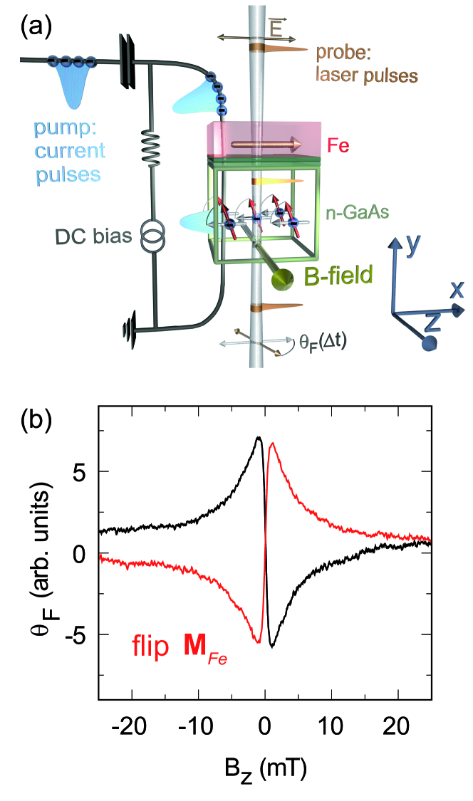
Figure 1: Electrical pump and optical probe setup and test by continuous electrical injection. (a) Schematic of the electrical pump and optical probe experiment of spins injected from Fe into $n$-GaAs. (b) Faraday rotation $\theta_{F}$ (Hanle depolarisation) of the dc current along the $y$ direction as a function of the external transverse magnetic field $B_{z}$ at constant bias before (black line) and after (red line) flipping the Fe magnetization $\mathbf{M}_{Fe}$.

III Results

III.1 Static spin injection

We first use static measurements of the Faraday rotation to demonstrate electrical spin injection in our devices (Fig. 1b). The sample is reverse biased, i.e. positive voltage probe on GaAs, and spins are probed near the fundamental band gap of GaAs. At $B_{z}=0$ T, spins are injected parallel to the easy axis direction of the Fe layer yielding $\theta_{F}=0$. At small magnetic fields $B_{z}$, spins start to precess towards the $y$-direction yielding $\theta_{F}\neq 0$. $\theta_{F}$ is a direct measure of the resulting net spin component $S_{y}$. Changing the sign of $B_{z}$ inverts the direction of the spin precession which results in a sign reversal of $\theta_{F}$. As expected Crooker et al. (2005), the direction of spin precession also inverts when the magnetization direction of the Fe layer is reversed (see red curve in Fig. 1b). $\theta_{F}$ approaches zero at large fields, since the continuously injected spins dephase due to Larmor precession causing strong Hanle depolarisation.

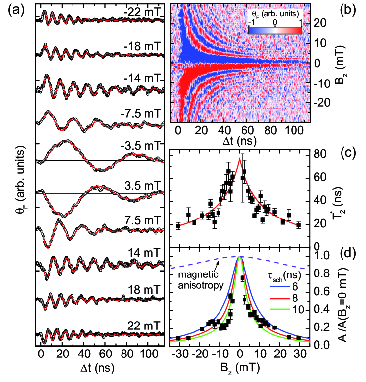
Figure 2: Pulsed electrical spin injection. (a) Time evolution of the Faraday rotation $\theta_{F}$ versus pump-probe delay $\Delta t$ for various magnetic fields $B_{z}$ with vertical offsets for clarity. Red lines are fits to the data for $\Delta t>\Delta w=2$ ns. (b) False color plot of $\theta_{F}$ versus $\Delta t$ and $B_{z}$. (c) Fitted spin dephasing time $T_{2}^{*}(B_{z})$ and (d) normalized oscillation amplitudes $A$ versus $B_{z}$ field. The error bars include the least-squares fit errors only. The red solid line in (c) is a least-squares fit to the data and solid lines in (d) are simulations for different effective charge and discharge times $\tau_{sch}$ of the Schottky barrier. The dashed line is the expected decrease of $A$ due to the magnetic anisotropy of the Fe injector layer.

III.2 Time-resolved spin injection

For time-resolved spin injection experiments, we now apply voltage pulses with a full width at half maximum of $\Delta w=2$ ns and a repetition time of $T_{rep}=125$ ns with $T_{rep}>T_{2}^{*}$. The corresponding time-resolved Faraday rotation data are shown in Figs. 2a and 2b at various magnetic fields. Most strikingly, we clearly observe Larmor precessions of the injected spin packets demonstrating that the voltage pulses trigger the macro-phase of the spin packets. It is apparent that the amplitude of $\theta_{F}$ is diminished with increasing $|B_{z}|$. We note that the oscillations in $\theta_{F}$ are not symmetric about the zero base line (see black lines in Fig. 2a as guides to the eye). For quantitative analysis we use

$$\theta_{F}(\Delta t,B_{z}) \propto M_{y}(\Delta t,B_{z})$$ (1)

$$= A(B_{z})\exp\left(-\frac{\Delta t}{T_{2}^{*}(B_{z})}\right)\sin(\omega_{L}\Delta t+\phi)$$

$$+ A_{bg}(B_{z})\exp\left(-\frac{\Delta t}{\tau_{bg}}\right),$$

with $\omega_{L}=g\mu_{B}B/\hbar$, where $g$, $\mu_{B}$ and $\hbar$ denote the effective electron $g$ factor, the Bohr magneton and the reduced Planck constant and $\phi$ being a phase factor. The second term accounts for the non-oscillatory time dependent background with a lifetime $\tau_{bg}$ and an amplitude $A_{bg}$ (The magnetic field dependence of $A_{bg}$ is shown in the Supplemental Material Sup ). The least-squares fits to the experimental data are shown in Fig. 2a as red curves. We determine a field independent $\tau_{bg}=8\pm 2$ ns and deduce $|g|=0.42\pm 0.02$ from $\omega_{L}$ as expected given that the spin precession is detected in the bulk $n$-GaAs layer Kikkawa and Awschalom (1998). The extracted spin dephasing times $T_{2}^{*}(B_{z})$ and amplitudes $A(B_{z})$ are plotted in Figs. 2c and 2d, respectively. The longest $T_{2}^{*}(B_{z})$ values, which exceed 65 ns, are obtained at small magnetic fields. The observed 1/B dependence of $T_{2}^{*}(B_{z})$ (see red line in Fig. 2c), which indicates inhomogeneous dephasing of the spin packet, is consistent with results obtained from all-optical time-resolved experiments on bulk samples with similar doping concentration Kikkawa and Awschalom (1998). On the other hand, the strong decrease of $A(B_{z})$ with magnetic field (Fig. 2d) has not previously been observed in all-optical experiments. Note that spin precession is barely visible for magnetic fields above 30 mT.

The $A(B_{z})$ dependence might be caused by the $B_{z}$ field acting on the direction of the magnetization $\mathbf{M}_{Fe}$ of the Fe injector. Increasing $B_{z}$ rotates $\mathbf{M}_{Fe}$ away from the easy ($x$-direction) towards the hard axis ($z$ direction) of the Fe layer. This rotation diminishes the $x$ component of the magnetization vector of the injected spin packet, which would result in a decrease of $A(B_{z})$. We calculated this dependence (see dashed line in Fig. 2d) for a macrospin $\mathbf{M}_{Fe}$ using in-plane magnetometry data from the Fe layer (see Fig. 6). The resulting decrease is, however, too small to explain our $A(B_{z})$ dependence.

To summarize, there are two striking observations in our time-resolved electrical spin injection experiments: (I) the strong decrease of the Faraday rotation amplitude $A(B_{z})$ and (II) the non-oscillatory background in $\theta_{F}(\Delta t)$ with a field independent time constant $\tau_{bg}=8\pm 2$ ns. As both have not been observed in time-resolved all-optical experiments, it is suggestive to link these properties to the dynamics of the electrical spin injection process.

In our time-resolved experiment, electron spin packets are injected across a Schottky barrier by short voltage pulses. The depletion layer at the barrier acts like a capacitance. When a voltage pulse is transmitted through the barrier, the capacitance will be charged and subsequently discharged. For studying the effect of the charging and discharging on the spin injection process, we performed high-frequency (HF) electrical characterization of our devices.

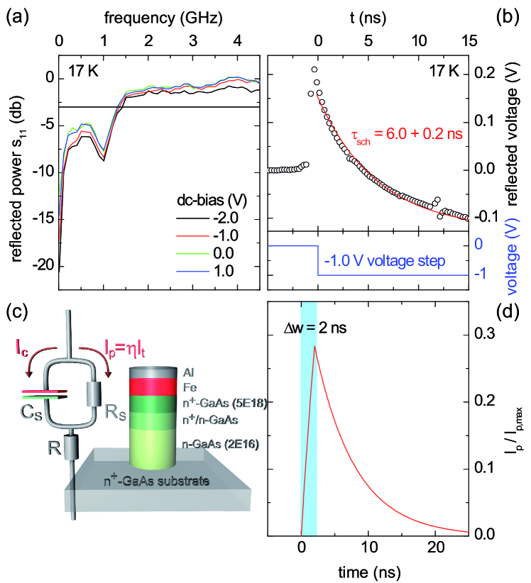
Figure 3: Electrical high frequency characterization. (a) Reflected power ($S_{11}$) for various dc-bias operating points obtained from vector network analysis. (b) Voltage reflected from the sample after applying a voltage step function (-1.0V) with least-squares exponential fit (red solid line). (c) Sample structure and simple equivalent network of the sample. (d) Simulation (red line) of the evolution of the spin-polarized tunnel current through the Schottky barrier triggered by a 2 ns long current pulse (light blue).

III.3 High-frequency sample characteristic

The HF bandwidth of the sample is deduced from the reflected electrical power $S_{11}$ by vector network analysis as shown in Fig. 3a. More than half of the electrical power ($S_{11}>3$ dB) is reflected from the device for frequencies above $\sim 1.5$ GHz. This bandwidth is independent of the operating point over a wide dc-bias range from -2.0 V (reverse biased Schottky contact) to 1.0 V and allows the sample to absorb voltage pulses of width $\Delta w\gtrsim 500$ ps.

Furthermore, the time evolution of the voltage drop at the Schottky barrier, i.e., its charging and discharging, can directly be determined by time-domain reflectometry (TDR). To analyse the charging dynamics of the Schottky capacitance, we apply a voltage step to the sample with an amplitude of -1 V and a rise time of 100 ps. The time-evolution of the reflected voltage step is shown in Fig. 3b. Note that there is a significant temporal broadening of the voltage step. We obtain a similar time constant for the discharging behaviour (not shown). Any impedance mismatch along the 50 $\Omega$ transmission line can be detected by measuring the time evolution of the reflected voltage. A real impedance above 50 $\Omega$ yields a reflected step function with negative amplitude. If the transmission line is terminated by a capacitance, the time evolution of the voltage drop during charging of the capacitance equals the time dependence of the reflected voltage. Note that even after 15 ns the voltage pulse is not fully absorbed by the sample, i.e. about 10 % of its amplitude is still being reflected. As long as the pulse is applied the absolute amplitude of the reflected voltage will rise towards saturation, which is reached at full charging up of the capacitance (Further information is provided in the Supplemental Material Sup ).

To further link the HF dynamics of the Schottky barrier to the pulsed electrical spin injection process, we depict a simple equivalent network of the sample in Fig. 3c. In the reverse-bias regime, the Schottky contact can be modeled by a Schottky capacitance $C_{s}$ and a parallel tunnel-resistance $R_{s}$. The underlying $n$-GaAs detection layer is represented by a resistance $R$ in series. We assume the displacement current $I_{c}$ to be unpolarized, while the tunneling current $I_{t}$ carries the spin polarized electrons. The spin current $I_{p}=\eta I_{t}$ is given by the spin injection efficiency $\eta$. The charging and discharging of the Schottky capacitance is thus directly mapped to the temporal evolution of the spin current. $I_{p}$ increases after the voltage pulse is turned on, whereas it decreases after the pulse is turned off after time $\Delta w$, i.e. during the discharge of $C_{s}$. If $C_{s}$, $R_{s}$ and $\eta$ are approximately bias-independent, the increase and decrease of $I_{p}$ is single-exponential

$$I_{p}(t)=I_{p,dc}\times\left\{\begin{array}[]{c|l}1-d\exp\left(-\frac{t}{\tau_{sch}}\right)&0\leq t<\Delta w\\ \left[\exp\left(\frac{\Delta w}{\tau_{sch}}\right)-d\right]\exp\left(-\frac{t}{\tau_{sch}}\right)&\Delta w\leq t<T_{rep}\end{array}\right.$$ (2)

and determined by the effective charge and discharge time $\tau_{sch}$ of the Schottky barrier as illustrated in Fig. 3d for a pulse width of $\Delta w=2$ ns and $\tau_{sch}=6$ ns. The constant $d=\left[\exp\left(\frac{\Delta w-T_{rep}}{\tau_{sch}}\right)-1\right]/\left[\exp\left(-\frac{T_{rep}}{\tau_{sch}}\right)-1\right]$ is given by the boundary condition $I_{p}(0)=I_{p}(T_{rep})$.

It is important to emphasize that the temporal width of the electrically injected spin packet is determined by $\tau_{sch}$. This temporal broadening becomes particularly important when individual spins start to precess in the external magnetic field at all times during the spin pulse. The retardation of spin precession results in spin dephasing of the spin packet. This phase ”smearing” leads to a decrease of the net magnetization. Its temporal evolution can be estimated by

$$M_{y}(B_{z},\Delta t)=\int\limits_{0}^{\Delta t}dt\ r_{S}(t)M_{0}(\Delta t-t),$$ (3)

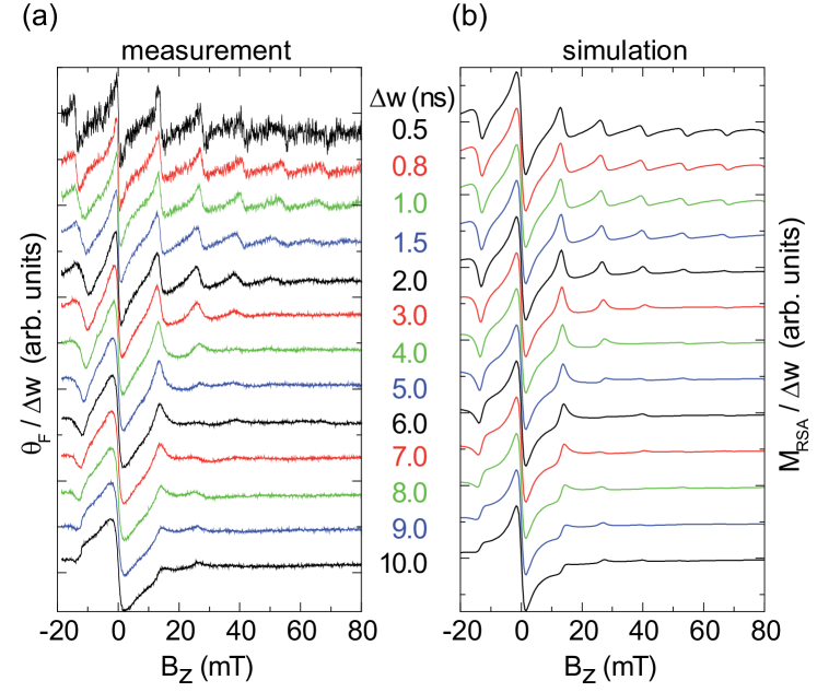
Figure 4: Resonant spin amplification for various voltage pulse widths $\Delta w$. (a) Measured Faraday rotation $\theta_{F}$ normalized to $\Delta w$ versus magnetic field $B_{z}$ at $T_{rep}=12.5$ ns and fixed $\Delta t$ with vertical offsets for clarity. (b) Simulations applying Eqs. 2 and 4 with $r_{s}(t)$ from Fig. 3d and $\tau_{sch}=6$ ns, $T_{2}^{*}=18$ ns.

where $r_{S}(t)=I_{p}(t)/a$ is the spin injection rate with the active sample area $a$ and where $M_{0}$ is given by an exponentially damped single spin Larmor precession. The integral can be solved analytically Sup and results in a form as given qualitatively by Eq. 1 describing the dynamics of the injected spin packets, assuming $I_{p}(0)=0$, i.e., $d=1$. Note that the non-precessing background signal of $\theta_{F}$ (see Fig. 2a) stems from the discharging of the Schottky capacitance, i.e. $\tau_{sch}=\tau_{bg}$, while $T_{2}^{*}$ is not affected by the integration. This assignment is confirmed by the independent determination of $\tau_{sch}$ by TDR. The amplitude $A(B_{z})$ in Eq. 1 becomes a function of $\omega_{L},T_{2}^{*},\tau_{sch},\Delta w$ and $r_{s}$ (see Eqs. S17 and S22 of the Supplemental Material Sup . For simulating $A(B_{z})$, we take the above fitting results from Fig. 2, i.e. $T_{2}^{*}(B_{z})$, $\omega_{L}$, as well as $\Delta w=2$ ns and vary only $\tau_{sch}$ as a free parameter. The resulting field dependent amplitudes are plotted in Fig. 2d at various time constants $\tau_{sch}$. The experimental data are remarkably well reproduced for the $\tau_{sch}$ values determined by TDR ($\tau_{sch}=6$ ns) and by the non-oscillatory background of $\theta_{F}$ ($\tau_{sch}=8$ ns). This demonstrates that the charging and discharging of the Schottky capacitance is the main source of the amplitude drop in our experiment.

III.4 Resonant spin amplification

We now analyse the precession of the spin packets after injection with voltage pulses of different width $\Delta w$. This can better be tested as a function of $B$ field instead of in the time domain. To enhance the signal-to-noise ratio of $\theta_{F}$, we reduce $T_{rep}$ to 12.5 ns. As $T_{rep}$ is now shorter than $T_{2}^{*}$, spin packets from subsequent voltage pulses can interfere. We thus enter the regime of resonant spin amplification (RSA)Kikkawa and Awschalom (1998); Kuhlen et al. (2014). The net RSA magnetization $M_{y,RSA}$ results with Eq. 3 in

$$M_{y,RSA}(B_{z},\Delta t) =M(\Delta t)$$ (4)

$$+\sum\limits_{n=1}^{\infty}\int\limits_{0}^{T_{rep}}dt\ r_{S}(t)M_{0}(\Delta t-t+nT_{rep}),$$

where $M_{RSA}$ and $r_{S}$ are periodic in $T_{rep}$ and defined in the time interval $[0,T_{rep})$. Constructive interference of subsequent spin packets leads to periodic series of resonances as a function of $B$, if a multiple of $1/T_{rep}$ equals the Larmor frequency:

$$z/T_{rep}=\omega_{L}/(2\pi),$$ (5)

where $z$ is an integer.

Fig. 4a shows RSA scans for $\Delta w$ ranging between 500 ps and 10 ns taken at fixed $\Delta t$ and normalized to $\Delta w$. Multiple resonances are observed for short $\Delta w\leq 2$ ns. The strong decrease of the resonance amplitudes with the increase of $|B_{z}|$ is consistent with the time-domain experiments (see Fig. 2). The number of resonances, which equals the number of Larmor precession cycles, subsequently decreases for broader current pulses. We observe a continuous crossover to the Hanle regime for the broadest pulses of $\Delta w=10$ ns $\sim T_{rep}=12.5$ ns, which is close to the dc-limit of spin injection as shown in Fig. 1b. This crossover strikingly demonstrates the phase triggering by the current pulses. While pulse-width induced phase smearing is observed above $\Delta w=1.5$ ns, there are no effects of the pulse width below 1.5 ns due to the finite $\tau_{sch}$. Remarkably, pulsed spin injection is possible for $\Delta w$ as short as 500 ps.

The RSA scans are simulated using Eqs. 2 and 4 with $\tau_{sch}=6$ ns and are depicted in Fig. 4b. The dependence on $B_{z}$ as well as the phase ”smearing” with increasing pulse width are well reproduced. Note that even the change of the RSA peak shape for higher order resonances is reproduced by the simulations, demonstrating that our model explains all salient features of the experiment.

IV Conclusion

In conclusion, we have shown that fast current pulses can trigger the macroscopic phase of spin packets electrically injected across an Fe/GaAs Schottky barrier. Current pulses having a width down to 500 ps trigger a spin imbalance observed as magnetic oscillations matching the effective electron g-factor of GaAs. Charging and discharging of the Schottky barrier yield a temporal broadening of the spin packets resulting in a partial dephasing during spin precession. This partial spin dephasing manifests itself in a characteristic decrease of the oscillation amplitude as a function of the magnetic field and as a non-oscillating exponential decrease of the injected spin-magnetization. Our model fully captures both of these features, which have not appeared when using ultra-fast laser pulses for optical spin orientation, and it predicts that the time constant of the decreasing background is given by the discharging time constant of the Schottky barrier. This time constant independently determined by time-domain reflectometry well matches our observations of the phase smearing of the spin packet. Using a ten time higher frequency of the current pulses, we superimpose injected spin packets in GaAs and enter the regime of resonant spin amplification, which is well-covered by our model as well. Our model predicts that the phase smearing can be significantly suppressed by reduction of the the Schottky capacitance. In this respect spin injection from diluted magnetic semiconductors will be advantageous for realizing all-electrical coherent spintronic devices of high frequency bandwidth.

V Acknowledgments

Supported by HGF and by the Deutsche Forschungsgemeinschaft (DFG, German Research Foundation) under SPP 1285 (Grant no. 40956248). C.J.P and P.A.C acknowledge funding from the Office of Naval Research, the National Science Foundation (NSF) MRSEC program, the NSF NNIN program, and the University of Minnesota.

Appendix A Sample characteristics

This section provides additional information about the sample used in our experiment. The I-V characteristics are displayed in Fig. 5. Magnetometry data of the Fe injector can be found in Fig. 6

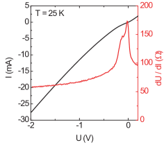
Figure 5: IV-characteristics. dc-current $I$ as a function of dc-bias $U$ (black line) and differential resistance $dU/dI$ (red line) of the sample with $1300$ $\mu$m diameter mesa at $25$ K. In our experiment, the Schottky diode is reverse-biased using short $-1.8$ V voltage pulses.

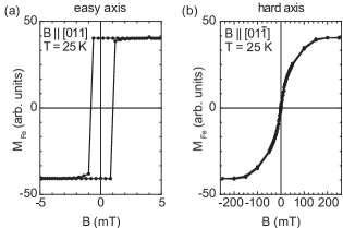
Figure 6: Magnetic anisotropy of the Fe injector layer. In-plane magnetization of the epitaxial iron injector layer $M_{Fe}$ as a function of the external magnetic field $B$ as determined from superconducting quantum interference device (SQUID) measurements at 25 K. The $B$-field is applied parallel to (a) the GaAs [011] and (b) the GaAs [01$\overline{1}$] crystal directions. The Fe injector layer exhibits an in-plane anisotropy. In our experiment, $B$ is applied nearly parallel to the GaAs [01$\overline{1}$] direction (hard axis).

Supplemental Material: Triggering phase-coherent spin packets by pulsed electrical spin injection across an Fe/GaAs Schottky barrier

Appendix S1 Superposition of pulse sequences

In Fig. 2 of the main article, a repetition frequency of the pump/probe pulses of $T_{rep}=125$ ns is used. At a repetition frequency of $T_{rep}=12.5$ ns (Fig. 4), which is lower than the spin coherence time $T_{2}^{*}$, the injected spin pulses start to superimpose and we observe resonant spin amplification. Here we consider a repetition period $T_{rep}=125$ ns for the probe laser-pulse. In addition to the electrical pump pulse at $\Delta t=0$, up to four additional current pulses can be applied each delayed by an additional 25 ns, while the repetition of probe pulses is kept at $125$ ns. Hence, we observe the superposition of injected spin packets in the time domain. First, we apply pump pulses with a repetition period of $25$ ns and choose $B=6.6$ mT for the magnetic field, such that the Larmor period equals the pump-pulse period: Sequential spin packets constructively superimpose and we enter the resonant spin amplification regime (Fig. S1a). The period of the $\theta_{F}$ signal equals the pump repetition frequency as expected. In Fig. S1b, we leave out the last two pump pulses of the sequence within the $125$ ns probe period. Accordingly, we observe the rise of the magnetization due to the constructive superposition of the first three spin-polarized current pulses in the first half of the probe-pulse period, followed by a decrease of the magnetization due to dephasing of the spin packets in the second half of the probe-pulse period.

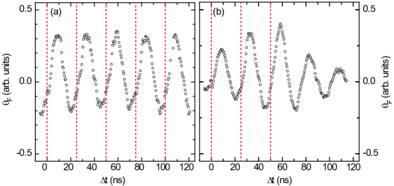
Fig. S1: Superposition of pulse sequences. Measured Faraday rotation $\theta_{F}$ as a function of the pump-probe delay $\Delta t$. The repetition frequency is set to $T_{rep}=125$ ns, $\Delta w=2$ ns and $B=6.6$ mT. (a) The probe pulse repetition is set to $T_{rep}=125$ ns and excitation pulses are applied at $\Delta t={0,25,50,75,100}$ ns (marked by red dashed vertical lines). (b) Same as in panel a, but only three excitation pulses are applied at $\Delta t={0,25,50}$ ns (marked by red dashed vertical lines).

Appendix S2 Model and derivations

In this section, we derive the fit Eq. 1 of the article from the ansatz Eq. 3. This calculation yields the expression of the simulated decrease of the Faraday rotation amplitude $A(B)$ as a function of the transverse magnetic field $B$ as plotted in Fig. 2d of the article.

Our model is based on the equivalent circuit diagram (Fig. 3c of the article), in which the Schottky contact is replaced by a capacitance $C_{s}$ and a parallel resistance $R_{s}$. The spin-polarized current $I_{p}(t)$ from the Fe-injector into the semiconductor is only transmitted by the tunnel current $I_{t}(t)$ through the Schottky resistance $R_{S}$. The displacement current $I_{c}(t)$ through the capacitance is assumed to be unpolarized. In order to determine $I_{p}(t)$, we use a local model neglecting runtime effects, since the distance of the elements in the equivalent circuit diagram is by far smaller than the electric AC wavelength used. From Fig. 1 it can be deduced that the Schottky contact in the reverse bias regime ($U<0$ V) is mainly ohmic. Since we use voltage pulses with an amplitude as high as $-1.8$ V, we can for simplicity neglect the weak bias-dependence of the tunnel resistance. When an external negative bias pulse of width $\Delta w$ is applied to the sample at time $t=0$, the Schottky capacitance starts to charge. If we assume for simplicity that the magnitude of the capacitance is constant, the $I_{t}(t)$ through the parallel resistor starts to rise exponentially and approaches the tunnel current $I_{t,dc}$, at which the Schottky capacitance would be fully charged. When the applied external bias is switched off at time $t=\Delta w$, the Schottky capacitance starts to discharge. This yields an exponential decrease of the voltage dropping across the parallel resistance $R_{S}$, and thus the tunnel current $I_{t}$ decreases exponentially with the characteristic decay time denoted $\tau_{sch}$. If we further assume that the spin injection efficiency $\eta$ is bias-independent, the polarized current is $I_{p}(t)=\eta I_{t}(t)$. In the case of a dc-bias applied to the sample, the spin injection rate reaches its maximum value $I_{p,dc}=\eta I_{t,dc}$. Hence, if a single voltage pulse is applied starting at time $t=0$, the polarized current is

$$I_{p}(t)=I_{p,dc}\times\left\{\begin{array}[]{c|l}1-d\exp\left(-\frac{t}{\tau_{sch}}\right)&0\leq t<\Delta w\\ \left[\exp\left(\frac{\Delta w}{\tau_{sch}}\right)-d\right]\exp\left(-\frac{t}{\tau_{sch}}\right)&\Delta w\leq t<T_{rep}\end{array}\right.$$ (S1)

with the time constant $\tau_{sch}$ for charging and discharging the Schottky capacitance. The constant $d$ is determined by the boundary conditions, i.e. the charging state of the Schottky capacitor, when the next current pulse arrives. For example, for a pulse repetition time $T_{rep}$ much longer than $\tau_{sch}$, the Schottky capacitor is fully discharged and the spin-polarized current is $I_{p}(0)=I_{p}(T_{rep})=0$ and hence $d=1$. The time-evolution of the voltage dropping at the sample and thus $\tau_{sch}$ can be determined directly from time-domain reflectometry as plotted in Fig. 3b of the article.

Now, we calculate the effect of the time-dependent polarized current $I_{p}(t)$ on the time-evolution of the observed Faraday rotation signal $\theta_{F}(\Delta t,B)$ in a transverse magnetic field $B$. The precession of a coherent spin packet in a transverse magnetic field is observed by its magnetization $\mathbf{M}$. Let us start the calculation with the simple case of a purely coherent spin injection, i.e. all spins are injected exactly at the same time, with a magnetization denoted by $\mathbf{M}_{0}$. This case is relevant for optical spin orientation by an ultra-short laser pulse, which is much shorter than the Larmor precession period of the oriented electron spins. Since the electrically injected spins are pumped perpendicular to the observation direction, which is determined by the probe laser beam, $\theta_{F}(\Delta t)$ is then proportional to $M_{0}^{\bot}(\Delta t,B)$

$$M_{0}^{\bot}(\Delta t,B)\propto\exp\left(-\frac{\Delta t}{T_{2}^{*}}\right)\sin\left(\omega_{L}\Delta t\right),$$ (S2)

where $\Delta t$, $T_{2}^{*}$, $\omega_{L}$ denote the pump-probe delay, the spin dephasing time, the Larmor frequency, respectively. Using a complex $M_{0}(\Delta t,B)$ with $M_{0}^{\bot}(\Delta t,B)=\Im(M_{0}(\Delta t,B))$, the calculation becomes independent of the observation direction:

$$M_{0}(\Delta t,B)\propto\exp\left(-\frac{\Delta t}{T_{2}^{*}}\right)\exp\left(i\omega_{L}\Delta t\right).$$ (S3)

The proportionality factor depends on the number of injected electrons and the magnetic moment of a single electron. It does not depend on the external magnetic field $B$.

Now, we take into account that the spins are injected slowly compared to the Larmor precession frequency. Thus, the first electron spins already precess, when further electrons are injected in the direction given by the static magnetisation of the iron layer. The probe laser measures the total magnetization $M$ induced by the injected spins, by $\theta_{F}$:

$$M(\Delta t,B) \propto \int_{0}^{\Delta t}I_{p}(t)\exp\left(-\frac{\Delta t-t}{T_{2}^{*}}\right)\exp\left(i\omega_{L}(\Delta t-t)\right)\ dt$$ (S4)

$$\propto \exp\left(-\frac{\Delta t}{T_{2}^{*}}+i\omega_{L}\Delta t\right)\int_{0}^{\Delta t}I_{p}(t)\exp\left(\frac{t}{T_{2}^{*}}-i\omega_{L}t)\right)\ dt$$

$$\propto M_{0}(\Delta t,B)\int_{0}^{\Delta t}I_{p}(t)M_{0}(-t,B)\ dt.$$

Despite its closed form, Eq. S4 is a complex integral over retarded purely coherent spin precessions $M_{0}(t,B)$, which is not suitable for data fitting. In the experiment, however, we observe the precessing net magnetization of the total injected spin ensemble by the Faraday rotation of the probe beam. In the following, our goal is to transform Eq. S4 to Eq. 1 of the article used to fit the measured $\theta_{F}(\Delta t,B)$ signal.

We start discussing $M(\Delta t,B)$ separately during the charging ($0\leq\Delta t<\Delta w$) and discharging ($\Delta w\leq\Delta t<T_{rep}$) process of the Schottky contact and define:

$$M(\Delta t,B)=\left\{\begin{array}[]{c|l}M_{cha}(\Delta t,B)&0\leq\Delta t<\Delta w\\ M_{dis}(\Delta t,B)&\Delta w\leq\Delta t<T_{rep}\end{array}\right.$$ (S5)

It follows with Eq. S1 and S4 (here $d=1$)

$$M_{cha}(\Delta t,B) \propto I_{p,dc}M_{0}(\Delta t,B)\int\limits_{0}^{\Delta t}\left[1-\exp\left(-\frac{t}{\tau_{sch}}\right)\right]M_{0}(-t,B)\ dt$$

$$M_{dis}(\Delta t,B) \propto I_{p,dc}M_{0}(\Delta t,B)\int\limits_{0}^{\Delta w}\left[1-\exp\left(-\frac{t}{\tau_{sch}}\right)\right]M_{0}(-t,0)\ dt+$$ (S6)

$$+I_{p,dc}M_{0}(\Delta t,B)\int\limits_{\Delta w}^{\Delta t}\left[\left(\exp\left(\frac{\Delta w}{\tau_{sch}}\right)-1\right)\exp\left(-\frac{t}{\tau_{sch}}\right)\right]M_{0}(-t,B)\ dt$$

$$=: M_{dis}^{(1)}(\Delta t,B)+M_{dis}^{(2)}(\Delta t,B)$$

Note that we replace $I_{p}(t)$ by the spin injection rate $r_{S}(t)=I_{p}(t)/a$ with the active sample area $a$ in the main article. We absorb here the $B$-independent factor $a$ in the proportionality factor. In the following, we consider only the net magnetization $M_{dis}(\Delta t,B)$ during the discharge of the capacitance ($\Delta t\geq\Delta w$) following the spin injection process for $0\leq\Delta t<\Delta w$, when the external bias is applied. This approach is sufficient, since only the domain $\Delta t\in[\Delta w,T_{rep})$ is used for the least-square fits in Fig. 2a of the article.

For compact writing, we define the real constant factor

$$f=I_{p,dc}\left(\exp\left(\frac{\Delta w}{\tau_{sch}}\right)-1\right),$$ (S8)

which is independent of $B$ and leave out the explicit $B$-dependence of $M_{0}(t,B)=M_{0}(t)$. First, we transform the second summand $M_{dis}^{(2)}(\Delta t,B)$ into a precessing net magnetization. Therefore, it is useful to introduce a timescale $\Delta t^{\prime}=\Delta t-\Delta w$:

$$M_{dis}^{(2)}(\Delta t^{\prime},B) \propto f\ M_{0}(\Delta t^{\prime}+\Delta w)\int\limits_{\Delta w}^{\Delta t^{\prime}+\Delta w}\exp\left(-\frac{t}{\tau_{sch}}\right)M_{0}(-t)\ dt$$

$$\propto f\ M_{0}(\Delta t^{\prime}+\Delta w)\int\limits_{0}^{\Delta t^{\prime}}\exp\left(-\frac{t+\Delta w}{\tau_{sch}}\right)M_{0}(-t-\Delta w)\ dt$$

Making use of the relation $M_{0}(-t-\Delta w)=\exp(\Delta w/T_{2}^{*}-i\omega_{L}\Delta w)\ M_{0}(-t)$ according to Eq. S3, we can further simplify the equation:

$$M_{dis}^{(2)}(\Delta t^{\prime},B) \propto f\exp\left(-\frac{\Delta w}{\tau_{sch}}\right)M_{0}(\Delta t^{\prime})\exp\left(\frac{-\Delta w}{T_{2}^{*}}\right)\int\limits_{0}^{\Delta t^{\prime}}\exp\left(-\frac{t}{\tau_{sch}}\right)M_{0}(-t)\exp\left(\frac{\Delta w}{T_{2}^{*}}\right)\ dt$$ (S9)

$$\propto f\exp\left(-\frac{\Delta w}{\tau_{sch}}\right)M_{0}(\Delta t^{\prime})\int\limits_{0}^{\Delta t^{\prime}}\exp\left(-\frac{t}{\tau_{sch}}\right)M_{0}(-t)\ dt$$

$$\propto I_{p,dc}\left(1-\exp\left(-\frac{\Delta w}{\tau_{sch}}\right)\right)M_{0}(\Delta t^{\prime})\int\limits_{0}^{\Delta t^{\prime}}\exp\left(-\frac{t}{\tau_{sch}}\right)M_{0}(-t)\ dt$$

$M_{dis}^{(2)}(\Delta t^{\prime},B)$ denotes the total precessing magnetization at time $\Delta t^{\prime}$, if spins are injected with an exponentially damped injection rate starting at $\Delta t^{\prime}=0$. Hence, it is due to the exponentially damped tail of the polarized current in Fig. 3d of the main article. In order to simplify $M_{dis}^{(2)}(\Delta t^{\prime},B)$, we briefly neglect the $B$ and $\Delta t^{\prime}$-independent real prefactor and focus on solving the integral and write for brevity $\gamma=1/T_{2}^{*}$ and $\lambda=1/\tau_{sch}$:

$$M_{dis}^{(2)}(\Delta t^{\prime},B) \propto M_{0}(\Delta t^{\prime})\int\limits_{0}^{\Delta t^{\prime}}\exp\left(-\lambda t\right)M_{0}(-t)\ dt$$

$$\propto \exp\left((i\omega_{L}-\gamma)\Delta t^{\prime}\right)\int\limits_{0}^{\Delta t^{\prime}}\exp\left((\gamma-\lambda-i\omega_{L})t\right)\ dt$$

$$\propto \frac{\exp\left((i\omega_{L}-\gamma)\Delta t^{\prime}\right)}{\gamma-\lambda-i\omega_{L}}\left[\exp((\gamma-\lambda-i\omega_{L})\Delta t^{\prime})-1\right]$$

$$\propto \frac{1}{\gamma-\lambda-i\omega_{L}}\left[\exp(-\lambda\Delta t^{\prime})-\exp((-\gamma+i\omega_{L})\Delta t^{\prime})\right]$$

Since we observe the spins by Faraday rotation parallel to the $y$-direction and thus perpendicular to their original polarization direction in the Fe layer (parallel to $x$-direction), we are interested in $M_{dis}^{\bot(2)}(\Delta t^{\prime},B)=\Im\left(M_{dis}^{(2)}(\Delta t^{\prime},B)\right)$, which results in

$$M_{dis}^{\bot(2)}(\Delta t^{\prime},B) \propto \frac{\omega_{L}e^{-\lambda\Delta t^{\prime}}}{(\gamma-\lambda)^{2}+\omega_{L}^{2}}-\frac{\gamma e^{-\gamma\Delta t^{\prime}}\sin(\omega_{L}\Delta t^{\prime})}{(\gamma-\lambda)^{2}+\omega_{L}^{2}}+\frac{\lambda e^{-\gamma\Delta t^{\prime}}\sin(\omega_{L}\Delta t^{\prime})}{(\gamma-\lambda)^{2}+\omega_{L}^{2}}-\frac{\omega_{L}e^{-\gamma\Delta t^{\prime}}\cos(\omega_{L}\Delta t^{\prime})}{(\gamma-\lambda)^{2}+\omega_{L}^{2}}$$

$$\propto \frac{\omega_{L}}{(\gamma-\lambda)^{2}+\omega_{L}^{2}}\left[e^{-\lambda\Delta t^{\prime}}-e^{-\gamma\Delta t^{\prime}}\left(\cos(\omega_{L}\Delta t^{\prime})+\frac{\gamma-\lambda}{\omega_{L}}\sin(\omega_{L}\Delta t^{\prime})\right)\right]$$

$$\propto \frac{1/\omega_{L}}{\Gamma^{2}+1}\left[e^{-\lambda\Delta t^{\prime}}-e^{-\gamma\Delta t^{\prime}}\left(\cos(\omega_{L}\Delta t^{\prime})+\Gamma\sin(\omega_{L}\Delta t^{\prime})\right)\right].$$

In the last step, we introduced the unit-less constant for brevity:

$$\Gamma=\frac{\gamma-\lambda}{\omega_{L}}=\frac{1}{\omega_{L}}\left(\frac{1}{T_{2}^{*}}-\frac{1}{\tau_{sch}}\right).$$ (S11)

Adding the real prefactor from Eq. S9, we find finally:

$$M_{dis}^{\bot(2)}(\Delta t^{\prime},B) \propto \left(1-\exp\left(-\frac{\Delta w}{\tau_{sch}}\right)\right)\frac{I_{p,dc}}{\omega_{L}}\frac{1}{\Gamma^{2}+1}\times$$ (S12)

$$\times\left\{\exp\left(-\frac{\Delta t^{\prime}}{\tau_{sch}}\right)-\exp\left(-\frac{\Delta t^{\prime}}{T_{2}^{*}}\right)\left[\cos(\omega_{L}\Delta t^{\prime})+\Gamma\sin(\omega_{L}\Delta t^{\prime})\right]\right\}$$

.

All the $B$-field dependence of $M_{dis}^{\bot(2)}(\Delta t^{\prime},B)$ is given by $\omega_{L}$. The proportionality factor is still independent of $B$. Strikingly, the evolution of the calculated net magnetization in Eq. S12 is the sum of an exponentially decreasing background with the characteristic time constant $\tau_{sch}$ of the Schottky contact:

$$M_{bg}^{\bot(2)}(\Delta t^{\prime},B) = A_{bg}\exp\left(-\frac{\Delta t^{\prime}}{\tau_{sch}}\right)$$ (S13)

$$A_{bg} \propto \left(1-\exp\left(-\frac{\Delta w}{\tau_{sch}}\right)\right)\frac{I_{p,dc}}{\omega_{L}}\frac{1}{\Gamma^{2}+1}.$$ (S14)

and an exponentially damped oscillation $M_{osc}^{\bot(2)}(\Delta t^{\prime},B)$ with the time constant $T_{2}^{*}$ of the spins:

$$M_{osc}^{\bot(2)}(\Delta t^{\prime},B) \propto \left(1-\exp\left(-\frac{\Delta w}{\tau_{sch}}\right)\right)\frac{I_{p,dc}}{\omega_{L}}\frac{1}{\Gamma^{2}+1}\times$$ (S15)

$$\times\left\{-\exp\left(-\frac{\Delta t^{\prime}}{T_{2}^{*}}\right)\left[\cos(\omega_{L}\Delta t^{\prime})+\Gamma\sin(\omega_{L}\Delta t^{\prime})\right]\right\}$$

The latter can be expressed in terms of a net magnetization of a purely coherently injected spin packet $M_{0}^{\bot}(\Delta t,B)$ (Eq. S2) with an additional phase $\delta_{2}$:

$$M_{osc}^{\bot(2)}(\Delta t^{\prime},B)=A^{(2)}\exp\left(-\frac{\Delta t^{\prime}}{T_{2}^{*}}\right)\sin\left(\omega_{L}\Delta t^{\prime}+\delta_{2}\right),$$ (S16)

with the definitions

$$A^{(2)} \propto \left(1-\exp\left(-\frac{\Delta w}{\tau_{sch}}\right)\right)\frac{I_{p,dc}}{|\omega_{L}|}\frac{1}{\sqrt{\Gamma^{2}+1}}$$ (S17)

$$\tan\delta_{2} = 1/\Gamma$$ (S18)

$$\Delta t^{\prime} = \Delta t-\Delta w,$$ (S19)

where we used $\sin(\arctan(1/\Gamma))=1/\sqrt{\Gamma^{2}+1}$ and $\cos(\arctan(1/\Gamma))=\Gamma/\sqrt{\Gamma^{2}+1}$. Note that $\omega_{L}<0$ for an effective g-factor $g<0$ as it is the case for GaAs. Remarkably, the amplitude $A^{(2)}$ of the precessing net magnetization becomes a function of the absolute magnetic field $|B|$ because of $|\omega_{L}|$ and $\Gamma^{2}(\omega_{L})$ (see Eq. S11). For a vanishing Schottky capacitance $\tau_{sch}\rightarrow 0$, which yields a square-like pulsed $I_{p}(t)$, the summand $M_{osc}^{\bot(2)}$ vanishes due to $\Gamma\rightarrow\infty$ and $A^{(2)}\rightarrow 0$. This limit confirms the interpretation of $M_{osc}^{\bot(2)}$. A huge time constant $\tau_{sch}\rightarrow\infty$ suppresses the spin injection $I_{p}(t)\rightarrow 0$ (Eq. S1) and results consistently in $A^{(2)}\rightarrow 0$ due to the prefactor $\left(1-\exp\ (-\Delta w/\tau_{sch})\right)$ in Eq. S17.

Finally, we consider the first summand $M_{dis}^{(1)}(\Delta t,B)$ of Eq. S6. This can be expressed as

$$M_{dis}^{(1)}(\Delta t,B) = c(B)M_{0}(\Delta t,B)$$ (S20)

$$= c(B)\exp\left(-\frac{\Delta t}{T_{2}^{*}}\right)\exp\left(i\omega_{L}\Delta t\right)$$

$$M_{dis}^{\bot(1)}(\Delta t,B) = \Im\left(M_{dis}^{(1)}(\Delta t,B)\right)$$ (S21)

$$= A^{(1)}\exp\left(-\frac{\Delta t}{T_{2}^{*}}\right)\sin\left(\omega_{L}\Delta t+\delta_{1}\right)$$ (S22)

with a complex constant $c(B)$, which is the result of the integral in Eq. S6 and does not depend on $\Delta t$ but on $\Delta w$. To put it more clearly, the first summand of the net magnetization during the discharge of the capacitance $C_{s}$ ($\Delta t>\Delta w$) in Eq. S6 is a Larmor precession with frequency $\omega_{L}$, decay time $T_{2}^{*}$ starting with a phase $\delta_{1}$. The superposition of the exponentially damped oscillations $M_{dis}^{\bot(1)}(\Delta t,B)$ and $M_{osc}^{\bot(2)}(\Delta t,B)$ from Eq. S16 yield a new oscillation with amplitude $A(B)$ and phase $\delta(B)$. Regarding the exponential background (Eq. S14), the measured $\theta_{F}(\Delta t,B)\propto\mathfrak{Im}(M(\Delta t,B))$ is thus equivalent to the fitting formula Eq. 1 of the main article for the considered polarized current $I_{p}(t)$.

If the voltage pulse repetition time $T_{rep}$ is shorter than the spin dephasing time $T_{2}^{*}$ (see Fig. 4 of the main article), interference of subsequent voltage pulses has to be taken into account. In this case of resonant spin amplification, the ansatz Eq. 3 of the article has to be replaced by Eq. 4. The summation of the voltage pulses leads to resonant spin amplification and more complicated dependence of the amplitude and the phase of the oscillating net magnetization $M_{RSA}$ upon application of the transverse magnetic field. It is not surprising, that resonant spin amplification can also be observed, if the period of the probe $T_{rep,probe}$ is much larger than $T_{2}^{*}$, but the period of the pump $T_{rep,pump}$ is smaller than $T_{2}^{*}$ and fulfills the resonance condition $\frac{2\pi}{T_{rep,pump}}\approx\omega_{L}$ as shown in section S1 of the supplements. Note that the small positive shift in Faraday rotation $\theta_{F}$ in Fig. S1 originates from the effective non-oscillating background in Eq. S14. In fact, we can derive the magnetization dynamics of the resonant spin amplification case $M_{RSA}(\Delta t,B)$analogously to the case of a single pump pulse shown here, but have to solve for $d$ by the condition $I_{p}(0)=I_{p}(T_{rep})=I_{p}(T_{rep,pump})$ in Eq. S1:

$$d=\frac{\exp(\frac{\Delta w-T_{rep}}{\tau_{sch}})-1}{\exp(-\frac{T_{rep}}{\tau_{sch}})-1}.$$ (S23)

The result was used for the simulations shown in Fig. 4b of the main article.

Appendix S3 Magnetic field dependence of the background

In the main article, the magnetic field dependence of the amplitude $A(B_{z})$ of the oscillating component observed during time-resolved spin injection is compared to expectations from our model (Fig. 2d). Here, we discuss the magnetic-field dependence of the amplitude of the non-oscillating background $A_{bg}(B_{z})$ (shown in Fig. S2), which exponentially decays as a function $\Delta t$ as observed in Fig. 2a. Applying Eq. 1, $A_{bg}(B_{z})$ is extracted from the least-square fits of the $\theta_{F}(\Delta t)$ shown in Fig. 2a, of which the fitted parameters $|g|=0.42$ and $\tau_{bg}=8$ ns as well as $\tau_{sch}(B_{z})$ and $A(B_{z})$ were already discussed in the main article.

According to the model described in Section S2, $A_{bg}(B_{z})$ is given by Eq. S14 and parameterized by $|g|$, $\Delta w$, $\tau_{sch}$ and the magnetic field dependence of $\tau_{sch}(B_{z})$. We observe a good agreement of the expected curve with the fitted black data points (Fig. S2), if we use the same values for all the parameters $|g|=0.42$, $\Delta w=2$ ns, $\tau_{sch}\approx\tau_{bg}=8$ ns and $\tau_{sch}(B_{z})$ as extracted from the oscillating magnetic field component during time-resolved spin injection. The shape of $A_{bg}(B_{z})$ resembles a Hanle depolarization curve, but does not originate from continuous spin injection as in Fig. 1 of the main article. The origin here is that the current pulse triggers a magnetization, a part of which ($M_{dis}(\Delta t,B)$) can be written as a non-oscillating $M_{bg}^{\bot(2)}(\Delta t,B)$ (Eq. S13) and an oscillating $M_{osc}^{\bot(2)}(\Delta t,B)$ (Eq. S16) component.

Fig. S2: Magnetic field dependence of the background signal during pulsed spin injection. The parameter $A_{bg}$, determined from least-square fits of the measured Faraday rotation curves plotted in Fig. 2a of the main text is plotted as a function of the external magnetic field $B_{z}$. The error bars include the least-squares fit errors only. The red line represents the expected dependency with the determined parameters according to Eq. S14.

Appendix S4 Time domain reflectometry

For probing the charging dynamics of the Schottky contact discussed in Fig. 3b of the main article, we added a broadband 50 % power splitter to the otherwise unchanged setup (Fig. S3a) and recorded the voltage ($U_{ref}$) back-reflected from the sample together with a part of the voltage applied to the sample $U_{in}$ by a fast sampling scope. The observed total voltage $U_{tot}=U_{in}+U_{ref}$ (Fig. S3b) reveals the evolution of the voltage at the sample starting at $t=0$ s. As long as the voltage pulse is applied (total duration $\Delta w=264$ ns) the Schottky capacity charges up till the reflected voltage saturates. Its saturation value would correspond to $-0.9$ V$=U_{amp}$, if the parallel resistance $R_{S}$ to the Schottky capacitance was zero (open termination). The intentional drop of the absolute voltage at $t=0$ can be understood by charging up the fully uncharged Schottky capacitance. Note that a total voltage drop to zero is expected, if the parallel resistance $R_{S}$ to the Schottky capacitance is zero (shorted termination). The discharging of the Schottky capacitance starting at $t=264$ ns results in the reversed dynamics. In the inset of Fig. S3b, we compare time-domain reflectometry (here we used a pulse of $U_{amp}=-1$ V and $\Delta w=66$ ns) applied to the sample and to a broadband 50 Ohm impedance replacing the sample. In the latter case only the $U_{in}$ part of $U_{tot}$ is measured as expected.

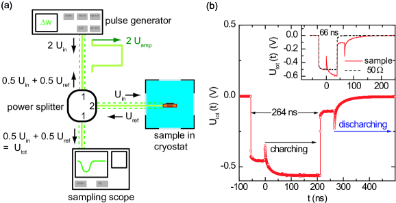
Fig. S3: Time domain reflectometry setup and measurement. (a) Set-up for time domain reflectometry. A pulse pattern generator sends a square pulse through a power splitter to the Fe/GaAs sample placed in the magneto-optical cryostat. The reflected voltage is measured by a sampling oscilloscope in the time-domain. (b) Time-domain reflectometry performed at 17 K on the Fe/GaAs mesa sample presented in the main article: The voltage $U_{tot}(t)=U_{in}(t)+U_{ref}(t)$ (red circles) is measured as a function of the time $t$ by a sampling oscilloscope. Here, we used a voltage pulse with an amplitude of $U_{amp}=-0.9$ V and a width of $\Delta w=264$ ns. $t=0$ ns correspond to the onset of the reflected signal. The Schottky capacitance starts to discharge at $t=264$ ns. The outcome of the measurement using $U_{amp}=-1.0$ V and $\Delta w=66$ ns is plotted in the inset (red solid line). The black dashed line shows the reflected pulse when using a broadband $50~{}\Omega$ termination replacing the Fe/GaAs sample.

References

- Hanson and Awschalom (2008) R. Hanson and D. D. Awschalom, Nature 453, 1043 (2008).
- Awschalom et al. (2002) D. D. Awschalom, D. Loss, and N. Samarth, eds., Semiconductor Spintronics and Quantum Computing (Springer-Verlag, Berlin, 2002).
- Kikkawa and Awschalom (1998) J. M. Kikkawa and D. D. Awschalom, Phys. Rev. Lett. 80, 4313 (1998).
- Kuhlen et al. (2014) S. Kuhlen, R. Ledesch, R. de Winter, M. Althammer, S. T. B. Gönnenwein, M. Opel, R. Gross, T. A. Wassner, M. S. Brandt, and B. Beschoten, Phys. Status Solidi B 251, 1861 (2014), ISSN 0370-1972.
- Schreiber et al. (2007a) L. Schreiber, D. Duda, B. Beschoten, G. Güntherodt, H.-P. Schönherr, and J. Herfort, phys. stat. sol. b 244, 2960 (2007a).
- Schreiber et al. (2007b) L. Schreiber, D. Duda, B. Beschoten, G. Güntherodt, H.-P. Schönherr, and J. Herfort, Phys. Rev. B 75, 193304 (2007b).
- Schmalbuch et al. (2010) K. Schmalbuch, S. Göbbels, Ph. Schäfers, Ch. Rodenbücher, P. Schlammes, Th. Schäpers, M. Lepsa, G. Güntherodt, and B. Beschoten, Phys. Rev. Lett. 105, 246603 (2010), ISSN 1079-7114.
- Kato et al. (2003) Y. K. Kato, R. C. Meyers, A. C. Gossard, and D. D. Awschalom, Nature 427, 50 (2003).
- Crooker and Smith (2005) S. A. Crooker and D. L. Smith, Phys. Rev. Lett. 94, 236601 (2005).
- Kuhlen et al. (2012) S. Kuhlen, K. Schmalbuch, M. Hagedorn, P. Schlammes, M. Patt, M. Lepsa, G. Güntherodt, and B. Beschoten, Phys. Rev. Lett. 109, 146603 (2012), ISSN 1079-7114.
- Stepanov et al. (2014) I. Stepanov, S. Kuhlen, M. Ersfeld, M. Lepsa, and B. Beschoten, Appl. Phys. Lett. 104, 062406 (2014), ISSN 0003-6951.
- Crooker et al. (2005) S. A. Crooker, M. Furis, X. Lou, C. Adelmann, D. L. Smith, C. J. Palmstrøm, and P. A. Crowell, Science 309, 2191 (2005).
- Kato et al. (2005) Y. K. Kato, R. C. Myers, A. C. Gossard, and D. D. Awschalom, Appl. Phys. Lett. 87, 022503 (2005), ISSN 0003-6951.
- Lou et al. (2007) X. Lou, C. Adelmann, S. A. Crooker, E. S. Garlid, J. Zhang, K. S. M. Reddy, S. D. Flexner, C. J. Palmstrøm, and P. A. Crowell, Nature Phys. 3, 197 (2007).
- Appelbaum et al. (2007) I. Appelbaum, B. Huang, and D. J. Monsma, Nature 447, 295 (2007), ISSN 1476-4687.
- Huang et al. (2007) B. Huang, D. J. Monsma, and I. Appelbaum, Phys. Rev. Lett. 99, 177209 (2007), ISSN 1079-7114.
- Li et al. (2008) J. Li, B. Huang, and I. Appelbaum, Appl. Phys. Lett. 92, 142507 (2008), ISSN 0003-6951.
- Ohno et al. (1999) Y. Ohno, D. K. Young, B. Beschoten, F. Matsukura, H. Ohno, and D. D. Awschalom, Nature 402, 790 (1999).
- Fiederling et al. (1999) R. Fiederling, M. Keim, G. Reuscher, W. Ossau, G. Schmidt, A. Waag, and L. W. Molenkamp, Nature 402, 787 (1999).
- Zhu et al. (2001) H. J. Zhu, M. Ramsteiner, H. Kostial, M. Wassermeier, H.-P. Schönherr, and K. H. Ploog, Phys. Rev. Lett 87, 016601 (2001).
- Hanbicki et al. (2002) A. T. Hanbicki, B. T. Jonker, G. Itskos, G. Kioseoglou, and A. Petrou, Appl. Phys. Lett. 80, 1240 (2002).
- Hanbicki et al. (2003) A. T. Hanbicki, O. M. J. van’t Erve, R. Magno, G. Kioseoglou, and C. H. Li, Appl. Phys. Lett. 82, 4092 (2003).
- Jiang et al. (2005) X. Jiang, R. Wang, R. M. Shelby, R. M. Macfarlane, S. R. Bank, J. S. Harris, and S. S. P. Parkin, Phys. Rev. Lett. 94, 056601 (2005).
- Adelmann et al. (2005) C. Adelmann, X. Lou, J. Strand, C. J. Palmstrøm, and P. A. Crowell, Phys. Rev. B 71, 121301R (2005).
- Kotissek et al. (2007) P. Kotissek, M. Bailleul, M. Sperl, A. Spitzer, D. Schuh, W. Wegscheider, C. H. Back, and G. Bayreuther, Nat. Phys. 3, 872 (2007), ISSN 1745-2481.
- Truong et al. (2009) V. G. Truong, P.-H. Binh, P. Renucci, M. Tran, Y. Lu, H. Jaffrès, J.-M. George, C. Deranlot, A. Lemaître, T. Amand, et al., Appl. Phys. Lett. 94, 141109 (2009), ISSN 0003-6951.
- Asshoff et al. (2009) P. Asshoff, W. Löffler, J. Zimmer, H. Füser, H. Flügge, H. Kalt, and M. Hetterich, Appl. Phys. Lett. 95, 202105 (2009), ISSN 0003-6951.
- Li et al. (2011) C. H. Li, O. M. J. van ’t Erve, and B. T. Jonker, Nat. Commun. 2, 1 (2011), ISSN 2041-1723.
- Hanbicki et al. (2012) A. T. Hanbicki, S.-F. Cheng, R. Goswami, O. M. J. van ’t Erve, and B. T. Jonker, Solid State Commun. 152, 244 (2012), ISSN 0038-1098.
- Schmidt et al. (2000) G. Schmidt, D. Ferrands, L. W. Molenkamp, A. T. Filip, and B. J. van Wees, Phys. Rev. B 62, R4790 (2000).
- Rashba (2000) E. I. Rashba, Phys. Rev. B 62, R16267 (2000).
- Kikkawa and Awschalom (1999) J. M. Kikkawa and D. D. Awschalom, Nature 397, 139 (1999).
- Dzhioev et al. (2002) R. I. Dzhioev, K. V. Kavokin, V. L. Korenev, M. V. Lazarev, B. Y. Meltser, M. N. Stepanova, B. P. Zakharchenya, D. Gammon, and D. S. Katzer, Phys. Rev. B 66, 245204 (2002).
- Crooker et al. (2007) S. A. Crooker, M. Furis, X. Lou, P. A. Crowell, D. L. Smith, C. Adelmann, and C. J. Palmstrøm, J. Appl. Phys. 101, 081716 (2007).
- (35) See Supplemental Material [URL will be inserted by publisher] for additional details on the modeling of the high frequency dynamics of the pulsed spin injection process based on the equivalent network of the sample presented in Fig. 3(c).