Abstract  Given a linear elliptic equation $\sum a_{ij}u_{ij}=0$ in $\mathbb{R}^{3}$, it is a classical problem to determine if its degree-one homogeneous solutions $u$ are linear. The answer is negative in general, by a construction of Martinez-Maure. In contrast, the answer is affirmative in the uniformly elliptic case, by a theorem of Han, Nadirashvili and Yuan, and it is a known open problem to determine the degenerate ellipticity condition on $(a_{ij})$ under which this theorem still holds. In this paper we solve this problem. We prove the linearity of $u$ under the following degenerate ellipticity condition for $(a_{ij})$, which is sharp by Martinez-Maure example: if $\mathcal{K}$ denotes the ratio between the largest and smallest eigenvalues of $(a_{ij})$, we assume $\mathcal{K}|_{\mathcal{O}}$ lies in $L_{\rm loc}^{1}$ for some connected open set $\mathcal{O}\subset\mathbb{S}^{2}$ that intersects any configuration of four disjoint closed geodesic arcs of length $\pi$ in $\mathbb{S}^{2}$. Our results also give the sharpest possible version under which an old conjecture by Alexandrov, Koutroufiotis and Nirenberg (disproved by Martinez-Maure’s example) holds.

1.  Introduction

Let $u\in C^{2}(\mathbb{R}^{3}\setminus\{0\})$ be a degree-one (positively) homogeneous solution to the linear equation

(1.1) $$\sum_{i,j=1}^{3}a_{ij}u_{ij}=0,\hskip 28.45274pta_{ij}\in L^{\infty}(\mathbb{R}^{3}),$$

in $\mathbb{R}^{3}$, i.e., $u(\rho x)=\rho u(x)$ for all $\rho>0$, $x\in\mathbb{R}^{3}$. Assume that (1.1) is elliptic, i.e.,

(1.2) $$(a_{ij}(x))$$ is positive definite

for every $x\in\mathbb{R}^{3}$. Note that the $a_{ij}$ are not continuous. Must then $u$ be a linear function?

This is a classical question motivated by global surface theory. Using an equivalent formulation, Alexandrov proved in 1939 that the answer is affirmative if $u$ is real analytic ([1]), and conjectured that an affirmative answer should also hold in the general case ([2], p. 352). The validity of this conjecture remained elusive for a long time, until Martinez-Maure [11] constructed in 2001 a striking $C^{2}$ counterexample to it. Specifically, he proved the existence of a nonlinear function $h\in C^{2}(\mathbb{S}^{2})$ such that the hedgehog $\psi(\nu):=\nabla h(\nu)+h(\nu)\nu:\mathbb{S}^{2}\rightarrow\mathbb{R}^{3}$ has negative curvature at its regular points. The homogeneous extension of degree one $u$ to $\mathbb{R}^{3}$ of $h$ gives a counterexample to Alexandrov’s conjecture. See Figure 1.1.

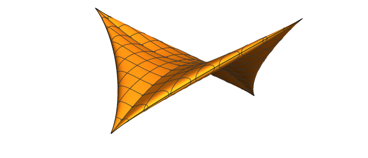
Figure 1.1. Martinez-Maure’s hegdehog $\nabla u(\mathbb{S}^{2})$, where $u$ solves (1.1)-(1.2). The preimage in $\mathbb{S}^{2}$ of each of the four horns of the example is a geodesic semicircle.

In contrast, in 2003 Han, Nadirashvili and Yuan [6] proved that the Alexandrov conjecture holds in the uniformly elliptic case. This solved an open problem by Safonov [19]. Specifically, if $0<\lambda(x)\leq\Lambda(x)$ are the smallest and largest eigenvalues of $(a_{ij}(x))$, and we denote $\mathcal{K}(x):=\Lambda(x)/\lambda(x)\geq 1$, Han, Nadirashvili and Yuan imposed the condition

(1.3) $$\mathcal{K}\in L^{\infty}(\mathbb{R}^{3})$$

and proved the following remarkable result:

Theorem 1.1 ([6]).

Any $1$-homogeneous solution $u\in W^{2,2}_{\rm loc}(\mathbb{R}^{3})$ to (1.1)-(1.3) is linear.

An alternative proof of Theorem 1.1 was obtained in 2016 by Guan, Wang and Zhang [5], again under very weak regularity assumptions on $u$. For that, they treated the problem directly as a uniformly elliptic equation in $\mathbb{S}^{2}$, and gave an elegant argument using the Bers-Nirenberg unique continuation theorem. A different approach to Theorem 1.1 via Poincaré-Hopf index theory was given by the authors and Tassi in [4]. The problem of the linearity of homogeneous solutions to (1.1)-(1.2) is discussed in detail in the book [13] by Nadirashvili, Tkachev and Vladut.

The uniform ellipticity assumption (1.3) in Theorem 1.1 cannot be weakened to plain ellipticity (1.2), by Martinez-Maure’s example. A known natural open problem proposed by Guan, Wang and Zhang (see [5, Remark 8]) is to establish what degenerate ellipticity conditions on the coefficients $a_{ij}$ are sufficient for Theorem 1.1 to hold, even when $u$ is smooth.

In this paper we give an answer to this problem. We explain next our main results.

Let $u\in C^{2}(\mathbb{R}^{3}\setminus\{0\})$ be a degree-one homogeneous solution to a linear equation (1.1). By homogeneity, $u$ also satisfies (1.1) for the coefficients $a_{ij}=a_{ij}(x/|x|)$. For this reason, our hypotheses on $(a_{ij})$ will be directly viewed at points $x\in\mathbb{S}^{2}$. Instead of (1.3), we will just assume that the considerably weaker condition

(1.4) $$\mathcal{K}|_{\mathcal{O}}\in L_{\rm loc}^{1}(\mathcal{O})$$

holds for some connected open set $\mathcal{O}\subset\mathbb{S}^{2}$ that it intersects any configuration of four disjoint geodesic semicircles (i.e. closed geodesic arcs of length $\pi$) in $\mathbb{S}^{2}$. Such a set $\mathcal{O}$ can be quite small. For instance, $\mathcal{O}$ can be chosen as any connected open set of $\mathbb{S}^{2}$ that contains an arbitrarily thin collar along a geodesic, $C_{\gamma}:=\{x\in\mathbb{S}^{2}:\langle x,\nu_{0}\rangle\in(0,\varepsilon)\}$ for some $\nu_{0}\in\mathbb{S}^{2}$, $\varepsilon>0$.

We prove:

Theorem 1.2.

Any $1$-homogeneous solution $u\in C^{2}(\mathbb{R}^{3}\setminus\{0\})$ to (1.1), (1.2), (1.4) is linear.

The four semicircles condition imposed on $\mathcal{O}$ is sharp. Indeed, Martinez-Maure’s example in [11] yields a $1$-homogeneous function $u\in C^{2}(\mathbb{R}^{3}\setminus\{0\})$ such that $D^{2}u$ is indefinite whenever it is non-zero, and so that $\{x\in\mathbb{S}^{2}:D^{2}u(x)=0\}$ agrees exactly with a certain configuration $\Gamma\subset\mathbb{S}^{2}$ of four disjoint geodesic semicircles. By the indefinite nature of $D^{2}u$, we can view $u$ as a solution to some elliptic equation (1.1)-(1.2), and the related function $\mathcal{K}$ associated to the coefficients $(a_{ij})$ of this equation lies in $L_{\rm loc}^{1}(\mathcal{O})$ for any open set $\mathcal{O}\subset\mathbb{S}^{2}$ disjoint from $\Gamma$.

We can actually prove a more general version of Theorem 1.2, that holds under degenerate ellipticity conditions:

Theorem 1.3.

Let $u\in C^{2}(\mathbb{R}^{3}\setminus\{0\})$ be a $1$-homogeneous solution to (1.1). Assume

(1.5) $$\left\{\begin{array}[]{l}\text{(i) $(a_{ij}(x))$ is semi-positive definite $\forall x\in\mathbb{R}^{3}$.}\\ \text{(ii) The restriction of $(a_{ij}(x))$ to the plane $x^{\perp}$ is non-zero, $\forall x\in\mathbb{R}^{3}-\{0\}$.}\\ \text{(iii) $(a_{ij})$ is positive definite a.e. on $\mathcal{O}$, and $\mathcal{K}|_{\mathcal{O}}\in L_{\rm loc}^{1}(\mathcal{O})$},\end{array}\right.$$

where, in $(iii)$, $\mathcal{O}\subset\mathbb{S}^{2}$ is some connected open set that intersects any configuration of four disjoint geodesic semicircles. Then, $u$ is linear.

Note that (i) extends (1.2) to the degenerate elliptic setting, and (ii) is needed in that general context to ensure that (1.1) is non-trivial when restricted to $1$-homogeneous functions.

The proof of Theorem 1.3 is a blend of geometric and analytic arguments, and is presented in Section 2. The idea, following Alexandrov [1], is to show that $\nabla u(\mathbb{S}^{2})$ reduces to a point, by analyzing the support planes in $\mathbb{R}^{3}$ of this compact set. In the uniformly elliptic case, Han, Nadirashvili and Yuan [6] used this idea and the maximum principle to show that $\nabla u(\mathbb{S}^{2})$ is a point. In our situation given by (1.5), we will use instead the Stoilow factorization for planar mappings of finite distortion [7, 3]. However, the main difficulty of the proof is that we are not assuming that $\mathcal{K}\in L^{1}(\mathbb{S}^{2})$, but only that its restriction to the possibly quite small set $\mathcal{O}\subset\mathbb{S}^{2}$ lies in $L_{\rm loc}^{1}$. In order to deal with this general situation, we will use an idea of Pogorelov [17]. In [17], Pogorelov claimed a proof of Alexandrov’s conjecture, something that is incorrect by the example in [11]. Pogorelov’s argument was based on the deep idea of controlling the connected components in which some suitable planes of $\mathbb{R}^{3}$ divide the saddle graph $\Sigma$ in $\mathbb{R}^{3}$ given by $z=u(x,y,1)$. However, this is a delicate question, and the short argument presented in [17] has several errors in the way these connected components are handled (one of them was pointed out in [15]). Our proof of Theorem 1.3 springs from Pogorelov’s brilliant idea, but we give a different, subtler argument that yields full control of the connected components mentioned above.

The term Alexandrov conjecture is often used in the literature in reference to a more general statement, in which (1.1) is allowed to be degenerate elliptic; see e.g. [11, 15, 13]. This conjecture admits several equivalent formulations, one of which is the following one, proposed in 1973 by Koutroufiotis and Nirenberg [8]:

The Alexandrov-Koutroufiotis-Nirenberg conjecture: Any $C^{2}$ function $v$ in $\mathbb{S}^{2}$ that satisfies ${\rm det}(\nabla_{\mathbb{S}^{2}}^{2}v)\leq 0$ at every point must be linear, i.e., $\nabla_{\mathbb{S}^{2}}^{2}v=0$.

Here, as usual, the spherical Hessian $\nabla_{\mathbb{S}^{2}}^{2}v$ is defined by $\nabla_{\mathbb{S}^{2}}^{2}v(q)=(v_{ij}(q)+v(q)\delta_{ij})$, where $v_{ij}$ are covariant derivatives with respect to a local orthonormal frame in $\mathbb{S}^{2}$, see e.g. [5]. We say that $v\in C^{2}(\mathbb{S}^{2})$ is a saddle function on $\mathbb{S}^{2}$ if it satisfies ${\rm det}(\nabla_{\mathbb{S}^{2}}^{2}v)\leq 0$. The conjecture is then that saddle functions on $\mathbb{S}^{2}$ are linear.

The support function $h$ of Martinez-Maure’s hedgehog in [11] gives a $C^{2}$ counterexample to this conjecture. Panina’s construction in [15] provides $C^{\infty}$ counterexamples, which are actually linear in large open regions of $\mathbb{S}^{2}$. Based on these results, Nadirashvili, Tkachev and Vladut proposed in [13, Conjecture 1.6.1] a lopped version of the conjecture, which can be rephrased as follows: any $C^{2}$ saddle function on $\mathbb{S}^{2}$ is linear in some open set.

This beautiful conjecture in [13] is open if $v$ is at least of class $C^{3}$, but in the general $C^{2}$ category, one should reformulate it slightly. Indeed, Martinez-Maure’s saddle function $h\in C^{2}(\mathbb{S}^{2})$ satisfies that $\{q\in\mathbb{S}^{2}:\nabla_{\mathbb{S}^{2}}^{2}h(q)=0\}$ is the union of four disjoint geodesic semicircles; in particular, $h$ is not linear on any open set of $\mathbb{S}^{2}$. Thus, the best possible lopped conjecture that can hold in the general $C^{2}$ case is that any saddle function $v\in C^{2}(\mathbb{S}^{2})$ always satisfies $\nabla_{\mathbb{S}^{2}}^{2}v=0$ along four disjoint geodesic semicircles. We will prove this exact result as a part of our proof of Theorem 1.3; see Section 3.

Theorem 1.4.

Let $v\in C^{2}(\mathbb{S}^{2})$ satisfy ${\rm det}(\nabla_{\mathbb{S}^{2}}^{2}v)\leq 0$. Then $\nabla_{\mathbb{S}^{2}}^{2}v=0$ along four disjoint geodesic semicircles of $\mathbb{S}^{2}$.

Theorem 1.4 gives then the sharpest possible version for which the conjecture by Alexandrov, Koutroufiotis and Nirenberg is true, i.e., the sharpest possible linearity theorem for saddle $C^{2}$ functions in $\mathbb{S}^{2}$. We should note that Panina claimed in [16] a very general statement that would have Theorem 1.4 as a particular case. However, the very short argument given in [16] is not correct; for instance, it relies on Pogorelov’s incorrect study of the connected components problem. In Theorem 3.1 we will give an alternative formulation of Theorem 1.4, in the context of the Weingarten inequality $(\kappa_{1}-c)(\kappa_{2}-c)\leq 0$ for ovaloids of $\mathbb{R}^{3}$.

The Alexandrov conjecture has been linked by Mooney [12] to the existence of Lipschitz minimizers to functionals $\int F(\nabla u)dx$ in $\mathbb{R}^{3}$, with $F$ strictly convex, that are $C^{1}$ except at a finite number of points. It has also been linked in [6, 13, 14] to the classification of degree-two homogeneous solutions to elliptic Hessian equations $F(D^{2}u)=0$ in $\mathbb{R}^{3}$. In particular, our results here might be of interest regarding the following conjecture in the book by Nadirashvili, Tkachev and Vladut, see [13, Conjecture 1.6.3]: a degree-two homogeneous smooth solution $u$ to a degenerate elliptic Hessian equation $F(D^{2}u)=0$ in $\mathbb{R}^{3}$ must be a quadratic polynomial.

The authors are grateful to Yves Martinez-Maure for enlightening comments and discussions.

2.  Proof of Theorem 1.3

Let $u\in C^{2}(\mathbb{R}^{3}\setminus\{0\})$ be a degree-one homogeneous solution to (1.1), where (1.5) holds. We will assume throughout the proof that $u$ is not linear, i.e. $D^{2}u$ is not identically zero on $\mathbb{R}^{3}$, and reach a contradiction. We will split the proof into several steps.

Step 1: Connection with quasiregular mappings.

In this step we relate the conditions in (1.5) with the theory of planar mappings with finite distortion, in order to apply the Stoilow factorization by Iwaniec-Sverak [7] to our context.

Consider arbitrary Euclidean coordinates $(x,y,z)$ in $\mathbb{R}^{3}$ centered at the origin, and define $h\in C^{2}(\mathbb{R}^{2})$ by

(2.1) $$h(x,y):=u(x,y,1).$$

Note that $u(x,y,z)=zh(x/z,y/z)$ for all $z>0$, by homogeneity. Then we have (see [6])

(2.2) $$\nabla u(x,y,1)=(h_{x},h_{y},h-xh_{x}-yh_{y})$$

and

(2.3) $$D^{2}u(x,y,1)=\left(\begin{array}[]{ccl}~h_{xx}&h_{xy}&-xh_{xx}~-yh_{xy}\\ &h_{yy}&-xh_{xy}-yh_{yy}\\ &*&x^{2}h_{xx}+2xyh_{xy}+y^{2}h_{yy}\end{array}~\right).$$

From here and the invariance of (1.1) by Euclidean isometries we see that the restriction of (1.1) to points of the form $(x,y,1)$ turns into a linear PDE for $h$,

(2.4) $$A_{11}h_{xx}+2A_{12}h_{xy}+A_{22}h_{yy}=0.$$

Specifically, if we denote $\mathcal{A}:=(a_{ij}(x,y,1))$ and $\mathcal{M}:=(A_{ij}(x,y))$, by (2.3), the coefficients of (2.4) are given for $i,j\in\{1,2\}$ by

(2.5) $$A_{ij}=w_{i}\cdot\mathcal{A}\cdot w_{j}^{T},$$

where $w_{1}:=(1,0,-x)$ and $w_{2}:=(0,1,-y)$. In other words, the bilinear form defined by $\mathcal{M}$ is the restriction of the one given by $\mathcal{A}$ to the plane of $\mathbb{R}^{3}$ orthogonal to $(x,y,1)$. By (i) and (ii) in (1.5), the matrix $\mathcal{M}$ is semi-positive definite and non-zero for all $(x,y)$. This clearly implies by (2.4) that, for any $(x,y)$,

(2.6) $$h_{xx}h_{yy}-h_{xy}^{2}\leq 0.$$

The converse of this property also holds, i.e., if $h(x,y)$ satisfies (2.6), it solves a degenerate elliptic equation (2.4) in $\mathbb{R}^{2}$, for adequate coefficients $A_{ij}$; see e.g. [18] for a similar argument in the elliptic case. Hence, if for any Euclidean linear coordinate system $(x,y,z)$, the function $h(x,y)$ given by (2.1) satisfies (2.6), then $u$ solves a linear equation (1.1) whose coefficients $a_{ij}$ satisfy (i), (ii) in (1.5).

Consider the smallest and largest eigenvalues $\lambda\leq\Lambda$ among the three eigenvalues of $\mathcal{A}$ at $(x,y,1)$, and let $\lambda_{1}\leq\lambda_{2}$ denote the eigenvalues of $\mathcal{M}$. By (2.5), we have

(2.7) $$0\leq\lambda\leq\lambda_{1}\leq\lambda_{2}\leq\Lambda.$$

Choose next a point $\nu_{0}\in\mathcal{O}\subset\mathbb{S}^{2}$ with positive $z$-coordinate, and express it as

(2.8) $$\nu_{0}=\frac{1}{\sqrt{1+x_{0}^{2}+y_{0}^{2}}}(x_{0},y_{0},1).$$

Since $(a_{ij})$ is positive definite a.e. on $\mathcal{O}$ by (iii) in (1.5), the matrix $\mathcal{M}$ is positive definite a.e. around $(x_{0},y_{0})$, by (2.7). Dividing by $A_{11}+A_{22}$, we can rewrite (2.4) as

(2.9) $$2h_{w\bar{w}}+\mu h_{ww}+\overline{\mu}h_{\bar{w}\bar{w}}=0$$

around $w_{0}:=x_{0}+iy_{0}$, where $w=x+iy$ and

(2.10) $$\mu=\frac{A_{11}-A_{22}+2iA_{12}}{A_{11}+A_{22}}.$$

Thus,

(2.11) $$|\mu|=\frac{K_{\mu}-1}{K_{\mu}+1}<1,\hskip 14.22636pt\text{ where }\hskip 14.22636ptK_{\mu}:=\frac{\lambda_{2}}{\lambda_{1}}\geq 1.$$

If we now write $f:=h_{w}$, then by (2.9) and (2.11) we have

(2.12) $$|f_{\bar{w}}|\leq|\mu||f_{w}|,\hskip 28.45274pt~|\mu|<1\text{ a.e. around $w_{0}$}.$$

Let us control next the dilatation quotient of $f$. If we denote

$$J(w,f):=|f_{w}|^{2}-|f_{\bar{w}}|^{2}\geq 0,\hskip 28.45274pt|Df(w)|:=|f_{w}|+|f_{\bar{w}}|,$$

the dilatation quotient of $f$ is given for any $w\in\mathbb{C}$ with $J(w,f)\neq 0$ by

$$K(w,f)=\frac{|Df(w)|^{2}}{J(w,f)}\geq 1.$$

At the points where $|Df(w)|=J(w,f)=0$, we define $K(w,f):=1$. Thus, $K(w,f)$ is defined a.e. around $w_{0}$, and by (2.11) and (2.12) we have at points with $J(w,f)\neq 0$

(2.13) $$K(w,f)\leq\frac{(|f_{w}|+|\mu||f_{w}|)^{2}}{|f_{w}|^{2}-|\mu|^{2}|f_{w}|^{2}}=\frac{(1+|\mu|)^{2}}{1-|\mu|^{2}}=K_{\mu}.$$

Hence, it follows from (2.7), (2.13) and our initial hypothesis $\mathcal{K}|_{\mathcal{O}}\in L_{\rm loc}^{1}(\mathcal{O})$, see (1.5)-(iii), that $K(w,f)\in L^{1}$ in a neighborhood of the point $w_{0}=x_{0}+iy_{0}\in\mathbb{C}$. To see this, recall that by definition, $\mathcal{K}=\Lambda/\lambda$. Thus, we are in the conditions of the Iwaniec-Sverak theorem for degenerate elliptic quasiregular mappings ([7], see also [3]), which provides a Stoilow factorization for $f$ in a neighborhood of $w_{0}$. This implies that, around $w_{0}$, $f$ is either constant or an open mapping. We summarize this conclusion in the following assertion for later use:

Assertion 2.1.

If $\nu_{0}=\frac{1}{\sqrt{1+x_{0}^{2}+y_{0}^{2}}}(x_{0},y_{0},1)$ lies in $\mathcal{O}\subset\mathbb{S}^{2}$, then $\nabla h$ is either an open mapping or constant around $(x_{0},y_{0})$.

Step 2: Gradient mappings and support planes.

In Steps 2 through 9 of the proof of Theorem 1.3, we will let $u\in C^{2}(\mathbb{R}^{3}\setminus\{0\})$ be a degree one homogeneous solution to a linear equation (1.1), and only assume that the coefficients $a_{ij}$ of (1.1) satisfy the degenerate ellipticity conditions (i), (ii) in (1.5). That is, we will not use condition (iii) in (1.5).

By homogeneity, $D^{2}u(x)$ always has a trivial zero eigenvalue corresponding to the radial direction, for any $x\in\mathbb{R}^{3}\setminus\{0\}$. Denote by $\mu_{1}(x)\leq\mu_{2}(x)$ the other two eigenvalues. These are also the eigenvalues of the spherical Hessian $\nabla_{\mathbb{S}^{2}}^{2}v$ of the function $v:=u(x/|x|)\in C^{2}(\mathbb{S}^{2})$ at the point $\eta=x/|x|$, see e.g. [5]. Here, the spherical Hessian of $v$ is defined by $\nabla_{\mathbb{S}^{2}}^{2}v(\eta)=(v_{ij}(\eta)+v(\eta)\delta_{ij})$, where $v_{ij}$ are covariant derivatives with respect to a local orthonormal frame in $\mathbb{S}^{2}$. Then, the property that the coefficients $a_{ij}$ of (1.1) satisfy the degenerate ellipticity conditions i), ii) in (1.5) is equivalent to the fact that $\mu_{1}\mu_{2}\leq 0$ everywhere, i.e., to the fact that, on $\mathbb{S}^{2}$, ${\rm det}(\nabla_{\mathbb{S}^{2}}^{2}v)\leq 0.$ This follows from the argument indicated after equation (2.6).

Consider the hedgehog in $\mathbb{R}^{3}$ given by the restriction of the gradient mapping of $u$ to the unit sphere, $\nabla u:\mathbb{S}^{2}\rightarrow\mathbb{R}^{3}$. It can be regarded as a compact surface (with singularities) in $\mathbb{R}^{3}$, see [9]. By compactness, $\nabla u(\mathbb{S}^{2})$ admits a support plane in any direction, where here by a support plane in the direction $\xi\in\mathbb{S}^{2}$ we mean a plane $\Pi_{\xi}\subset\mathbb{R}^{3}$ orthogonal to $\xi$ that touches $\nabla u(\mathbb{S}^{2})$ at some point $q_{\xi}$, and so that $\langle\nabla u-q_{\xi},\xi\rangle\leq 0$ on $\mathbb{S}^{2}$. Observe that $\nabla u(\mathbb{S}^{2})$ cannot be constant, since $D^{2}u$ is not identically zero. Thus, for almost every direction $\xi\in\mathbb{S}^{2}$, the two associated support planes to $\xi$ and $-\xi$ are different, and each of them intersects $\nabla u(\mathbb{S}^{2})$ at a unique point.

Given arbitrary Euclidean coordinates $(x,y,z)$ in $\mathbb{R}^{3}$, the hedgehog $\nabla u:\mathbb{S}^{2}\rightarrow\mathbb{R}^{3}$ can be parametrized as the map in (2.2), for all $\nu\in\mathbb{S}^{2}$ with positive $z$-coordinate, that is,

(2.14) $$\psi(x,y):=\nabla u(\nu)=(h_{x},h_{y},h-xh_{x}-yh_{y}),$$

where

(2.15) $$\nu:=\frac{(x,y,1)}{\sqrt{1+x^{2}+y^{2}}}.$$

Recall that, by (2.6), $h_{xx}h_{yy}-h_{xy}^{2}\leq 0$. Obviously, $\psi(x,y)$ is an immersion with unit normal $\nu$ at the points where ${\rm det}(D^{2}h)<0$. We call these points regular points of the hedgehog. We should note that, although $\psi$ is at first only of class $C^{1}$, it can be easily checked using the inverse function theorem that any regular point $q$ of $\psi$ has a neighborhood $\mathcal{U}\subset\mathbb{R}^{2}$ such that $\psi(\mathcal{U})$ is a $C^{2}$ graph over an open set of its tangent plane at $q$. Thus, it makes sense to talk about the second fundamental form $II$ of (2.14) at regular points, and a computation from (2.14), (2.15) shows that

(2.16) $$II=\frac{-1}{\sqrt{1+x^{2}+y^{2}}}D^{2}h(x,y).$$

In particular, the hedgehog has negative curvature at its regular points, and therefore such points cannot arise as contact points of $\nabla u(\mathbb{S}^{2})$ with a support plane. Note that the hedgehog $\nabla u(\mathbb{S}^{2})$ is regular at a point $\nu\in\mathbb{S}^{2}$ if and only if the two non-trivial eigenvalues $\mu_{1}\leq\mu_{2}$ of $D^{2}u(\nu)$ are non-zero (and so, necessarily, of opposite signs), i.e. if and only if $D^{2}u(\nu)$ has rank $2$.

Definition 2.2.

We say that $p_{0}\in\nabla u(\mathbb{S}^{2})$ is a Pogorelov point if there exists a direction $\xi\in\mathbb{S}^{2}$ such that $\nabla u(\mathbb{S}^{2})\cap\Pi_{\xi}=\{p_{0}\}$, and $p_{0}\not\in\{\nabla u(\xi),\nabla u(-\xi)\}$.

Assertion 2.3.

There exists a Pogorelov point of $\nabla u(\mathbb{S}^{2})$.

Proof.

We first note that $\nabla u:\mathbb{S}^{2}\rightarrow\mathbb{R}^{3}$ has a regular point. Indeed, otherwise we would have $\mu_{1}\mu_{2}=0$ on $\mathbb{S}^{2}$. Thus, the function $f:=u|_{\mathbb{S}^{2}}$ would satisfy ${\rm det}(\nabla_{\mathbb{S}^{2}}^{2}f)=0$ everywhere on $\mathbb{S}^{2}$. By [8, Theorem 1], $f$ would be linear on $\mathbb{S}^{2}$. So, $u$ would also be linear, a contradiction.

Let then $\xi\in\mathbb{S}^{2}$ be a regular point of $\nabla u$. By slightly varying $\xi$, we can assume additionally that each of the support planes $\Pi_{\xi}$ and $\Pi_{-\xi}$ intersects $\nabla u(\mathbb{S}^{2})$ at a unique point, say $q_{1}$ and $q_{2}$. As $\nabla u(\xi)$ cannot lie in any of these two planes (by regularity), either $q_{1}$ or $q_{2}$ is a Pogorelov point for $\nabla u(\mathbb{S}^{2})$. ∎

Step 3: Setup for the rest of the proof.

We fix from now on a Pogorelov point $p_{0}\in\nabla u(\mathbb{S}^{2})$, with associated direction $\xi\in\mathbb{S}^{2}$. Take $\nu_{0}\in\mathbb{S}^{2}$ with $\nabla u(\nu_{0})=p_{0}$. We consider Euclidean coordinates $(x,y,z)$ with $\xi=(1,0,0)$ and $\nu_{0}=(\nu_{0}^{1},0,\nu_{0}^{3})$, with $\nu_{0}^{3}>0$. One should observe that $\nu_{0}$ is not uniquely determined by $\xi$, since the subset $(\nabla u)^{-1}(p_{0})$ of $\mathbb{S}^{2}$ might be large. As a matter of fact, we seek to show that it contains a geodesic semicircle. At this stage of the proof we will not require any additional information on $\nu_{0}$, but in Step 8 we will discuss how to choose it in a convenient way.

Since $\xi=(1,0,0)$, the support plane $\Pi_{\xi}$ leaves $\nabla u(\mathbb{S}^{2})$ on its left side, i.e., $\Pi_{\xi}$ is of the form $x=\mu_{\rm max}$, and

(2.17) $$\mu_{\rm min}\leq u_{x}(p)~\leq\mu_{\rm max}\hskip 28.45274pt~\forall p\in\mathbb{S}^{2},$$

for some values $\mu_{\rm min},\mu_{\rm max}\in\mathbb{R}$. The points $\nabla u(\pm\xi)$ do not lie in $x=\mu_{\rm max}$, since $p_{0}$ is a Pogorelov point. Thus, there exist $\mu_{0}<\mu_{\rm max}$ and $\varepsilon>0$ such that $u_{x}(p)\leq\mu_{0}$ for every $p\in B(\xi;\varepsilon)\cup B(-\xi;\varepsilon)$, where here $B(a;\varepsilon)$ denotes a geodesic ball in $\mathbb{S}^{2}$ of center $a$ and radius $\varepsilon$. By homogeneity, $u_{x}(x,y,z)\leq\mu_{0}$ on a subset of $\mathbb{R}^{3}$ of the form $x^{2}\geq\delta(y^{2}+z^{2})$ for some $\delta=\delta(\varepsilon)>0$.

From now on, let $\Sigma$ be the entire saddle graph in $\mathbb{R}^{3}$ given by $z=h(x,y)$, where $h$ is defined by (2.1); note that $\Sigma$ has non-positive curvature at every point, by (2.6). By (2.2) and the compactness of $\nabla u(\mathbb{S}^{2})$, we see that $\nabla h$ is uniformly bounded in $\mathbb{R}^{2}$. Moreover, by (2.17), (2.2) and the definition of $\mu_{0}$, we have

(2.18) $$\mu_{\rm min}\leq h_{x}(x,y)~\leq\mu_{\rm max},$$

for all $(x,y)\in\mathbb{R}^{2}$, and

(2.19) $$h_{x}(x,y)\leq\mu_{0}<\mu_{\rm max}~\hskip 28.45274pt\text{$\forall(x,y)\in\mathbb{R}^{2}$ with $x^{2}\geq\delta(y^{2}+1).$}$$

We will denote by $\Omega^{+}$ (for $x>0$) and $\Omega^{-}$ (for $x<0$) the two connected components of the set $x^{2}\geq\delta(y^{2}+1)$ in $\mathbb{R}^{2}$. Also, note that

(2.20) $$h_{x}(x_{0},0)=\mu_{\rm max},\hskip 28.45274pt~\text{ where }\nu_{0}=(\nu_{0}^{1},0,\nu_{0}^{3})=\frac{(x_{0},0,1)}{\sqrt{1+x_{0}^{2}}}.$$

We will use frequently in what follows the notation

(2.21) $$\varphi(x,y):=(x,y,h(x,y)).$$

Step 4: A transverse line $L_{n}^{*}$ to $\Sigma\cap\{y=0\}$ with almost maximum slope.

Consider a plane $\Pi$ given by $z=P(x,y):=ax+by+c$, with $a>\mu_{0}$. Then, for any $y_{0}\in\mathbb{R}$, we have by (2.19) and $a>\mu_{0}$ that the line $L_{y_{0}}\equiv\Pi\cap\{y=y_{0}\}$ is above (resp. below) the graph $z=h(x,y_{0})$ as $x\to\infty$ (resp. $x\to-\infty$). In this way, there exist points $x_{1}(y_{0})\leq x_{2}(y_{0})$ such that

(2.22) $$h(x,y_{0})>P(x,y_{0})\text{ for $x<x_{1}(y_{0})$,}\hskip 28.45274pt~h(x,y_{0})<P(x,y_{0})~\text{ for $x>x_{2}(y_{0})$.}$$

In particular, there exist points $(x_{1},0)\in\Omega^{-}$ and $(x_{2},0)\in\Omega^{+}$ such that $h(x,0)>P(x,0)$ for all $x\leq x_{1}$, and $h(x,0)<P(x,0)$ for all $x\geq x_{2}$.

Assertion 2.4.

There exist continuous curves $x=\alpha^{-}(y)$, $x=\alpha^{+}(y)$ in $\mathbb{R}^{2}$, which depend on the initial plane $\Pi$, such that $\alpha^{-}(0)=x_{1}$, $\alpha^{+}(0)=x_{2}$, and

(2.23) $$h(\alpha^{-}(y),y)>P(\alpha^{-}(y),y),\hskip 28.45274pt~h(\alpha^{+}(y),y)<P(\alpha^{+}(y),y),$$

for all $y\in\mathbb{R}$.

Proof.

Take $\bar{a}\in(\mu_{0},a)$ and denote by $\overline{\mu}_{\rm min}$ the minimum value of $h_{y}$ in $\mathbb{R}^{2}$. Choose $\lambda<0$ so that the half-line $\mathcal{L}_{\lambda}\subset\mathbb{R}^{2}$ given by $x=x_{1}+\lambda y$ for $y\geq 0$ is contained in $\Omega^{-}$. We can obviously choose $\lambda$ so that, additionally, $(a-\bar{a})\lambda<\overline{\mu}_{\rm min}-b$ holds. See Figure 2.1. Then, $\alpha^{-}(y):=x_{1}+\lambda y$ satisfies the first inequality in (2.23) for all $y\geq 0$; indeed, if $(x,y)\in\mathcal{L}_{\lambda}$, integrating $\nabla h$ along $\mathcal{L}_{\lambda}$, and using that $h(x_{1},0)>P(x_{1},0)$ together with the previous inequalities we have

$$h(x,y)>h(x_{1},0)+(\bar{a}\lambda+\overline{\mu}_{\rm min})y\ >P(x_{1},0)+(a\lambda+b)y=P(x,y).$$

The first inequality for $y<0$, and the second inequality in (2.23) are obtained similarly. This proves Assertion 2.4.

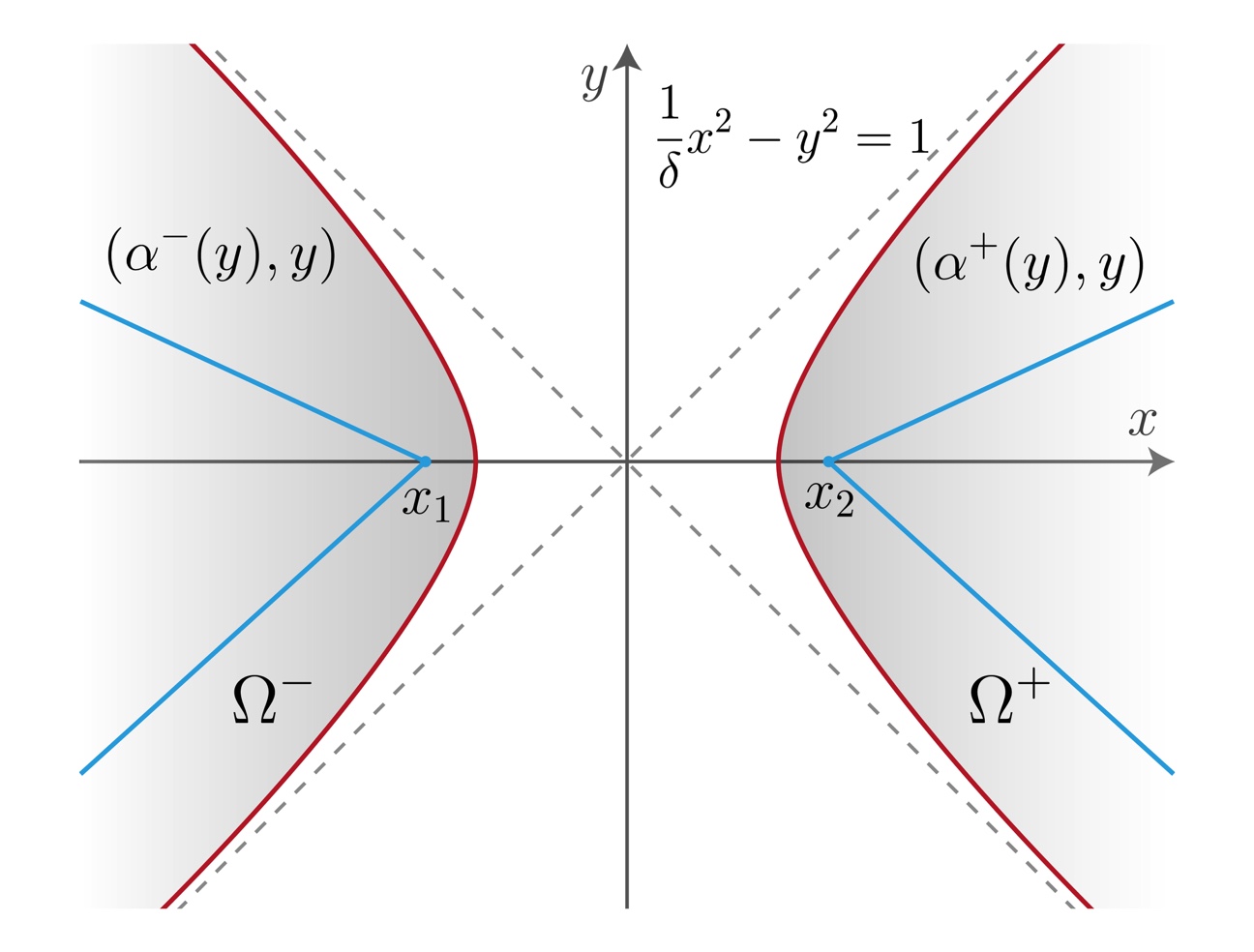
Figure 2.1. The curves $(\alpha^{\pm}(y),y)$ in $\mathbb{R}^{2}$.

∎

Remark 2.5.

Observe that, if we consider the continuous curves $x=\alpha^{\pm}(y)$ defined in Assertion 2.4 with respect to the plane $\Pi$, then all points $\varphi(x,y)\in\Sigma$ where $x<\alpha^{-}(y)$ (resp. $x>\alpha^{+}(y)$) lie above (resp. below) $\Pi$. In order to see this, it suffices to realize that the proof of Assertion 2.4 also holds if, instead of $(x_{1},0)\in\Omega^{-}$ we consider as initial point of $x=\alpha^{-}(y)$ any point $(x,0)$ with $x<x_{1}$ (and a similar argument for $x>x_{2}$ with $(x_{2},0)\in\Omega^{+}$).

Take next a sequence $\{\mu_{n}\}_{n}\to\mu_{\rm max}$, with $\mu_{n}\in(\mu_{0},~\mu_{\rm max})$ for all $n$. Consider the line $L_{n}$ in the vertical plane $y=0$ given by $z=\mu_{n}(x-x_{0})+h(x_{0},0)$. Note that $L_{n}$ intersects transversally $\Sigma_{0}:=\Sigma\cap\{y=0\}$ at $\varphi(x_{0},0)$, by (2.20). More specifically, since $\mu_{n}<~\mu_{\rm max}$, we see that $\Sigma_{0}$ lies below $L_{n}$ in the plane $y=0$ for values of $x<x_{0}$ near $x_{0}$, and above $L_{n}$ for $x>x_{0}$ near $x_{0}$. Besides, it is clear from (2.22) that $\Sigma_{0}$ lies above (resp. below) $L_{n}$ as $x\to-\infty$ (resp. as $x\to\infty$). This shows, in particular, that the planar set $\Sigma_{0}\setminus L_{n}$ has at least four connected components, each of them homeomorphic to an open interval.

By the transversality of $\Sigma_{0}$ and $L_{n}$ at $\varphi(x_{0},0)$, there exists some $\varepsilon>0$ such that $h_{x}(x,0)>\mu_{n}$ and $\varphi(x,0)\not\in L_{n}$ for all $x\neq x_{0}$ with $|x-x_{0}|<\varepsilon$. By Sard’s theorem, if necessary, we can make a small parallel translation of $L_{n}$ in the plane $y=0$, to obtain a new straight line $L_{n}^{*}$ which might not pass through $(x_{0},0,h(x_{0},0))$ anymore, but which intersects $\Sigma_{0}$ transversely at every intersection point. Specifically, we may take $L_{n}^{*}$ so that it contains a point $\varphi(x_{0}^{*},0)$ with $|x_{0}-x_{0}^{*}|<\varepsilon$, and so that the distance between $\varphi(x_{0}^{*},0)$ and $\varphi(x_{0},0)$ is smaller than $1/n$. Here, $x_{0}^{*}=x_{0}^{*}(n)$, i.e., $x_{0}^{*}$ depends on $n$.

Note that, by (2.22), $L_{n}^{*}$ lies either above or below $\Sigma_{0}$ as $x\to\infty$ or $x\to-\infty$. Then, by transversality, $\Sigma_{0}\setminus L_{n}^{*}$ has a finite number of connected components. By the above arguments, we also know that the number of such connected components is at least $4$, and that $\varphi(x_{0}^{*},0)$ lies at the common boundary of two such bounded connected components. We will use the following notations for some special connected components of $\Sigma_{0}\setminus L_{n}^{*}$; (see Figure 2.2).

1. $C_{\infty}^{+}$ is the unbounded component that lies strictly above $L_{n}^{*}$.

2. $C_{\infty}^{-}$ is the unbounded component that lies strictly below $L_{n}^{*}$.

3. $C_{0}^{+}$ is the bounded component that lies strictly above $L_{n}^{*}$, and has $\varphi(x_{0}^{*},0)$ as a boundary point.

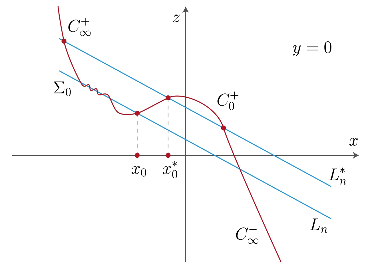
Figure 2.2. The connected components $C_{\infty}^{+}$, $C_{\infty}^{-}$ and $C_{0}^{+}$.

Observe that $C_{\infty}^{+}$ lies in the set $\{x<x_{0}^{*}\}$, while $C_{\infty}^{-}$ and $C_{0}^{+}$ lie in $\{x>x_{0}^{*}\}$

Step 5: Study of the intersection of $\Sigma$ with the sheaf of planes containing $L_{n}^{*}$.

Let us now fix the straight line $L_{n}^{*}$, and consider all the planes in $\mathbb{R}^{3}$, excluding $y=0$, that contain $L_{n}^{*}$. They are given by

(2.24) $$z=P_{b}(x,y)=\mu_{n}(x-x_{0}^{*})+by+h(x_{0}^{*},0),$$

for each $b\in\mathbb{R}$. Call $\Pi_{b}$ to the plane determined by $b$. We next study $\Sigma\cap\Pi_{b}$.

Fix some point $q_{0}\in C_{0}^{+}$. Let $I_{n}$ (resp. $J_{n}$) denote the set of values $b\in\mathbb{R}$ for which $q_{0}$ can be joined to a point $\varphi(x,y)\in\Sigma$, with $y>n$ (resp. with $y<-n$), through an arc contained in $\Sigma\setminus(\Pi_{b}\cup C_{\infty}^{+}).$ The statement of the next assertion uses that $\overline{\mu}_{\rm min}\leq h_{y}(x,y)\leq\overline{\mu}_{\rm max}$ for adequate constants, for all $(x,y)\in\mathbb{R}^{2}$. It states that for any $n\in\mathbb{N}$ there exists a plane $\Pi_{b_{n}}$ such that we can find an arc in $\Sigma$ joining $q_{0}$ to points $\varphi(x,y)$ where $y>n$ and $y<-n$, while avoiding both $\Pi_{b_{n}}$ and the connected component $C_{\infty}^{+}$.

Assertion 2.6.

There exists $b_{n}\in I_{n}\cap J_{n}$, with $\overline{\mu}_{\rm min}\leq b_{n}\leq\overline{\mu}_{\rm max}$.

Proof.

Write $q_{0}=\varphi(q_{0}^{1},0)$. By construction, $q_{0}$ lies above $L_{n}^{*}$. If we choose $b\leq\overline{\mu}_{\rm min}$, then $\varphi(q_{0}^{1},y)\in\Sigma$ lies above $\Pi_{b}$, for all $y>0$. Since $\varphi(q_{0}^{1},0)\not\in C_{\infty}^{+}$, this means that $\overline{\mu}_{\rm min}\in I_{n}$. By the same argument, $\overline{\mu}_{\rm max}\in J_{n}$. Thus $I_{n}$ and $J_{n}$ are non-empty, and they both intersect the closed interval $[\overline{\mu}_{\rm min},\overline{\mu}_{\rm max}]$.

We check next that $I_{n}$ is open. Let $b_{0}\in I_{n}$. Then, there exists an arc in $\Sigma\setminus(\Pi_{b_{0}}\cup C_{\infty}^{+})$ joining $q_{0}$ with a point $p=\varphi(x,y)$, with $y>n$. By compactness, this arc lies above $\Pi_{b_{0}}$ at a certain distance $d>0$. In particular, for values of $b$ near $b_{0}$, this arc also avoids $\Pi_{b}\cup C_{\infty}^{+}$. Therefore, $I_{n}$ is open. By the same argument, $J_{n}$ is open.

Finally, we prove that $I_{n}\cup J_{n}=\mathbb{R}$, what, together with the already proved properties and the fact that $[\overline{\mu}_{\rm min},\overline{\mu}_{\rm max}]$ is connected, yields Assertion 2.6. Arguing by contradiction, assume that there exists $b\in\mathbb{R}\setminus(I_{n}\cup J_{n})$. We are going to prove next that the (open) connected component of $\Sigma\setminus\Pi_{b}$ that contains $q_{0}$, which we will denote by $\Sigma(C_{0}^{+})$, is bounded. This will contradict the fact that $\Sigma$ is a saddle graph.

To do this, we start fixing some notation and making some elementary comments. First, note that $\Sigma(C_{0}^{+})$ lies above $\Pi_{b}$, since $q_{0}\in C_{0}^{+}$. Also, denote by $\Sigma(C_{\infty}^{+})$ the connected component of $\Sigma\setminus\Pi_{b}$ that contains $C_{\infty}^{+}$. By Remark 2.5, if we consider the continuous curves $x=\alpha^{\pm}(y)$ defined in Assertion 2.4 with respect to the plane $\Pi_{b}$, then all points $\varphi(x,y)\in\Sigma$ where $x<\alpha^{-}(y)$ (resp. $x>\alpha^{+}(y)$) lie above (resp. below) $\Pi_{b}$. In this way, the curve $\Gamma^{-}:=\{\varphi(\alpha^{-}(y),y)\in\Sigma:y\in\mathbb{R}\}$ is contained in $\Sigma(C_{\infty}^{+})$.

First of all, we prove that every point $\varphi(x,y)$ of $\Sigma(C_{0}^{+})$ satisfies $y\in[-n,n]$. Indeed, otherwise, there would exist an arc $\gamma$ in $\Sigma$ starting at $q_{0}$, that reaches either $\{y<-n\}$ or $\{y>n\}$, and that intersects $C_{\infty}^{+}$, since $b\not\in I_{n}\cap J_{n}$. Let $\overline{z}_{0}$ denote the first point where $\gamma$ touches $C_{\infty}^{+}$. Then, a neighborhood of $\overline{z}_{0}$ trivially lies in $\Sigma(C_{\infty}^{+})$. See Figure 2.3. In particular, $\Sigma(C_{\infty}^{+})=\Sigma(C_{0}^{+})$.

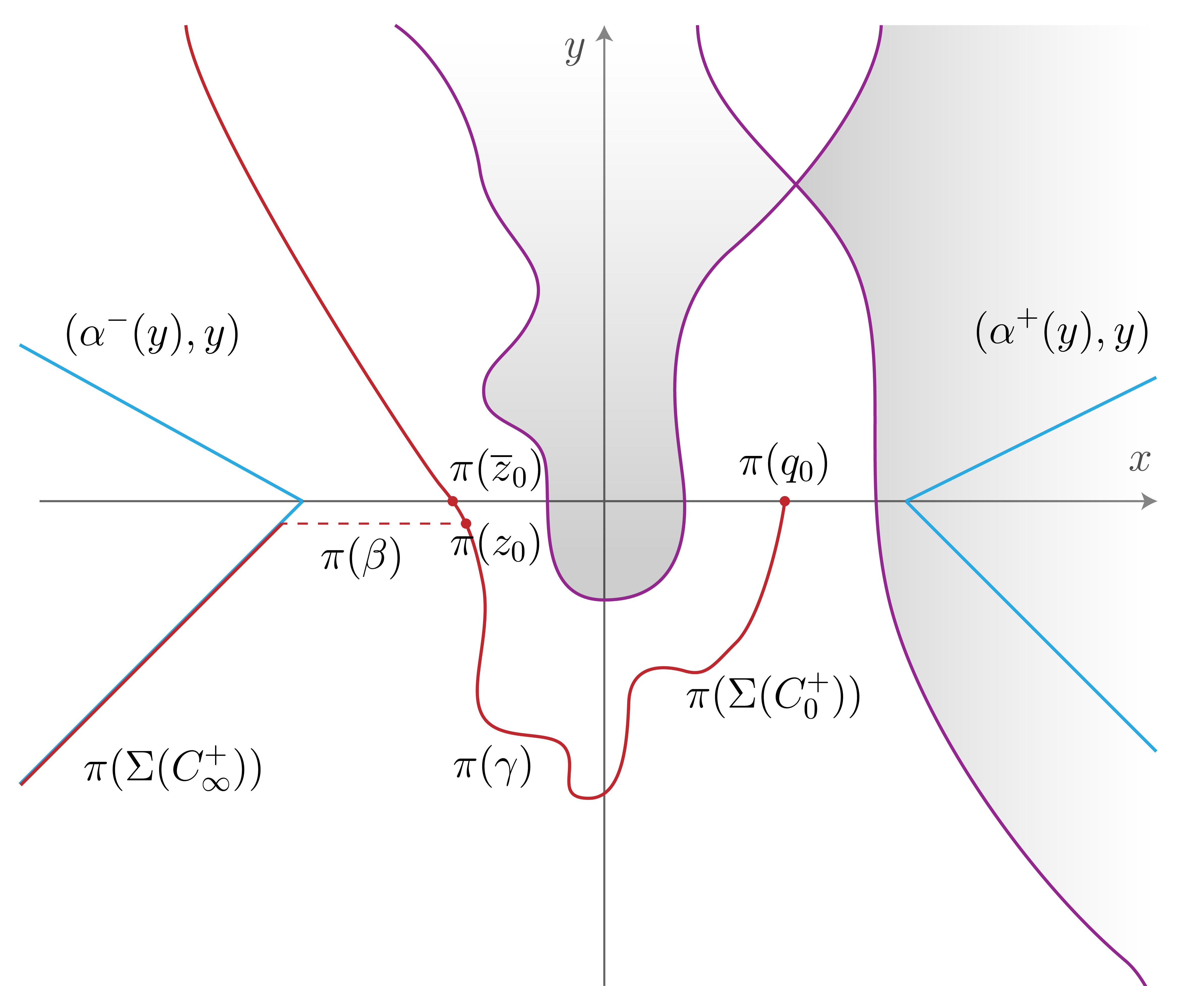
Figure 2.3. Proof that $\Sigma(C_{0}^{+})$ lies in the slab of $\mathbb{R}^{3}$ given by $|y|\leq n$. In the figure, $\pi$ denotes the projection $\pi(x,y,z)=(x,y)$ onto the $x,y$-plane

.

Let $z_{0}=\varphi(z_{0}^{1},z_{0}^{2})$ be a point of that neighborhood, that also lies in the interior of the arc of $\gamma$ between $q_{0}$ and $\overline{z}_{0}$. Assume that $z_{0}^{2}<0$ (the argument is similar if $z_{0}^{2}>0$). Then, we can join the curve $\Gamma^{-}\subset\Sigma$ defined above with the point $z_{0}$ along an arc $\beta$ contained in $\Sigma(C_{\infty}^{+})$ and so that every point of the arc $\beta$ has negative $y$-coordinate. See Figure 2.3. This implies that $\beta$ does not touch $C_{\infty}^{+}$, which is contained in the $y=0$ plane. Now, the union of the arc of $\gamma$ joining $q_{0}$ with $z_{0}$, the arc $\beta$, and a suitable arc of the curve $\Gamma^{-}$ produces an arc in $\Sigma(C_{\infty}^{+})$ that avoids $C_{\infty}^{+}$ and joins $q_{0}$ with a point in $\Sigma\cap\{y<-n\}$ (see Figure 2.3). This would mean that $b\in J_{n}$, a contradiction. Thus, $\Sigma(C_{0}^{+})$ lies in the slab of $\mathbb{R}^{3}$ given by $|y|\leq n$, as desired.

Recall that all points of the form $\varphi(\alpha^{+}(y),y)$ lie below $\Pi_{b}$, by Assertion 2.4. Since all points $\varphi(x,y)\in\Sigma(C_{0}^{+})$ satisfy $|y|\leq n$ and lie above $\Pi_{b}$, we conclude then that their $x$-coordinates are bounded from above by $\alpha^{+}(y)$.

On the other hand, assume that there exists an arc in $\Sigma(C_{0}^{+})$ that joins $q_{0}$ with a point of the form $\varphi(\alpha^{-}(y),y)$. By Assertion 2.4, we have $\Sigma(C_{0}^{+})=\Sigma(C_{\infty}^{+})$. But now, as $\Sigma(C_{\infty}^{+})$ has points of the form $\varphi(x,y)$ with $|y|$ arbitrarily large, we contradict the fact that $\Sigma(C_{0}^{+})$ lies in the slab $|y|\leq n$.

We have then proved that $\Sigma(C_{0}^{+})$ is contained in the compact set

$$\{\varphi(x,y):\alpha^{-}(y)\leq x\leq\alpha^{+}(y),|y|\leq n\}\subset\Sigma.$$

Thus $\Sigma(C_{0}^{+})$ is a bounded connected component of $\Sigma\setminus\Pi_{b}$, in contradiction with the saddleness of $\Sigma$. This proves Assertion 2.6. ∎

Step 6: Study of the intersection of $\Sigma$ with the limit plane $\Pi_{\infty}$.

For each $n$, let $b_{n}\in\mathbb{R}$ be given by Assertion 2.6, and consider the associated plane $\Pi_{b_{n}}$ given by (2.24) for $b=b_{n}$. Since $\overline{\mu}_{\rm min}\leq b_{n}\leq\overline{\mu}_{\rm max}$, we have up to subsequence that $\{b_{n}\}_{n}\to b_{\infty}\in[\overline{\mu}_{\rm min},\overline{\mu}_{\rm max}]$. Since $|x_{0}^{*}-x_{0}|<1/n$ and $\{\mu_{n}\}_{n}\to\mu_{\rm max}$, the planes $\Pi_{b_{n}}$ converge to the limit plane

(2.25) $$\Pi_{\infty}\hskip 5.69046pt~:\hskip 5.69046ptz=P_{\infty}(x,y):=\mu_{\rm max}(x-x_{0})+b_{\infty}y+h(x_{0},0),$$

which passes through $\varphi(x_{0},0)\in\Sigma$ with maximum slope $\mu_{\rm max}$ in the $x$-direction.

We study next $\Sigma\cap\Pi_{\infty}$. Fix any $y_{0}\in\mathbb{R}$. Then, taking $\Pi=\Pi_{\infty}$ in Assertion 2.4, it is a consequence of (2.23) that the curve $\Sigma\cap\{y=y_{0}\}$ intersects $\Pi_{\infty}$.

Assertion 2.7.

Either for all $y_{0}\geq 0$, or for all $y_{0}\leq 0$, there exist $x^{-}(y_{0})\leq x^{+}(y_{0})$ such that

$$\Pi_{\infty}\cap\Sigma\cap\{y=y_{0}\}=\{\varphi(x,y_{0}):x\in[x^{-}(y_{0}),x^{+}(y_{0})]\}.$$

Moreover, $h_{x}(x,y_{0})=\mu_{\rm max}$ holds for every $x\in[x^{-}(y_{0}),x^{+}(y_{0})]$, and $\Sigma$ lies above $\Pi_{\infty}$ (resp. below $\Pi_{\infty}$) when $x<x^{-}(y_{0})$ (resp. $x>x^{+}(y_{0})$).

Proof.

Fix $y_{0}\in\mathbb{R}$. We distinguish two possible situations.

Case 1: $\Pi_{\infty}\cap\Sigma\cap\{y=y_{0}\}$ is not a unique point. In that case, given two points $\varphi(x_{1},y_{0})$, $\varphi(x_{2},y_{0})$ of that intersection, we have that all points of the form $\varphi(x,y_{0})$ with $x\in[x_{1},x_{2}]$ also lie in $\Pi_{\infty}\cap\Sigma\cap\{y=y_{0}\}$. This follows since $h_{x}(x,y_{0})\leq\mu_{\rm max}=(P_{\infty})_{x}(x,y_{0})$ and $h(x_{i},y_{0})=P_{\infty}(x_{i},y_{0})$, for $i=1,2$. Thus, if $\Pi_{\infty}\cap\Sigma\cap\{y=y_{0}\}$ has at least two points, there exist $x^{-}(y_{0})<x^{+}(y_{0})$ such that:

1. $\varphi(x,y_{0})$ lies above $\Pi_{\infty}$ for all $x<x^{-}(y_{0})$.

2. $\varphi(x,y_{0})$ lies below $\Pi_{\infty}$ for all $x>x^{+}(y_{0})$.

3. $\varphi(x,y_{0})\in\Pi_{\infty}$ for all $x\in[x^{-}(y_{0}),x^{+}(y_{0})]$.

Note that $h_{x}(x,y_{0})=\mu_{\rm max}$ for all $(x,y_{0})$ in the third situation above. So, the statement of Assertion 2.7 holds for every $y_{0}\in\mathbb{R}$ such that $\Pi_{\infty}\cap\Sigma\cap\{y=y_{0}\}$ is not a unique point. No sign assumption is needed here for $y_{0}$.

Case 2: $\Pi_{\infty}\cap\Sigma\cap\{y=y_{0}\}$ is a unique point. This situation is subtler, and needs an additional control on the intersections $\Sigma\cap\Pi_{b_{n}}$ before passing to the limit.

Let $b_{n}$ be given by Assertion 2.6, with $\{b_{n}\}_{n}\to b_{\infty}$. By $b_{n}\in I_{n}\cap J_{n}$, there exists an arc $\gamma^{+}=\gamma^{+}(n)$ in $\Sigma$ that lies above $\Pi_{b_{n}}$, that does not intersect $C_{\infty}^{+}$, and whose endpoints have $y$-coordinate equal to $n$ and $-n$, respectively. Since $L_{n}^{*}$ intersects $\Sigma_{0}=\Sigma\cap\{y=0\}$ transversely at a finite number of points, there obviously exists a unique connected component $C_{1}^{-}$ of $\Sigma_{0}\setminus L_{n}^{*}$ that has as a boundary point the unique boundary point of $C_{\infty}^{+}$, and lies below $\Pi_{b_{n}}$ (since $C_{1}^{-}$ lies below $L_{n}^{*}$). As $\gamma^{+}$ lies above $\Pi_{b_{n}}$ and does not intersect $C_{\infty}^{+}$, we easily deduce that every point in $\gamma^{+}\cap\Sigma_{0}$ is of the form $\varphi(x,0)$, with $x>{\rm sup}\{x:\varphi(x,0)\in C_{1}^{-}\}$. Obviously, $\gamma^{+}\cap\Sigma_{0}$ is non-empty since $\gamma^{+}$ goes from $y=n$ to $y=-n$.

Let $\Sigma(C_{1}^{-})$ denote the connected component of $\Sigma\setminus\Pi_{b_{n}}$ that contains $C_{1}^{-}$ (thus, it lies below $\Pi_{b_{n}}$). For each $n$, let $\alpha_{n}^{+}(y)$, $\alpha_{n}^{-}(y)$ be the functions $\alpha^{+}(y),\alpha^{-}(y)$ defined by Assertion 2.4 with respect to $\Pi=\Pi_{b_{n}}$. Then, $\Sigma(C_{1}^{-})$ must intersect either $\Sigma\cap\{y=n\}$ or $\Sigma\cap\{y=-n\}$; indeed, otherwise, $\Sigma(C_{1}^{-})$ would be a connected component contained in a compact region of $\Sigma$ bounded by $\gamma^{+}$, $\Sigma\cap\{y=\pm n\}$ and $\{\varphi(\alpha_{n}^{-}(y),y):y\in\mathbb{R}\}$, and this contradicts the saddleness of $\Sigma$.

In this way, we can take an arc $\gamma^{-}=\gamma^{-}(n)$ contained in $\Sigma(C_{1}^{-})$ that joins a point of $C_{1}^{-}$ with a point $q_{n}$ of $\Sigma$ with $y$-coordinate equal to $n$ or $-n$. Up to a subsequence of the $\{b_{n}\}_{n}$, we can assume that one of these two situations holds for all $n$. For definiteness, we will assume that the $y$-coordinate of $q_{n}$ is equal to $n$, for all $n$.

Then, obviously, any plane $\{y=y_{0}\}$ with $y_{0}\in[0,n]$ is intersected by the curves $\gamma^{-}$, $\gamma^{+}$, and $\{\varphi(\alpha_{n}^{+}(y),y):y\in\mathbb{R}\}$. Using again that $\gamma^{+}\cap C_{\infty}^{+}=\emptyset$, we deduce the existence of points $x_{1}<x_{2}<\alpha_{n}^{+}(y_{0})$, with each $x_{1},x_{2}$ depending on $y_{0}$ and $n$, such that

$$\varphi(x_{1},y_{0})\in\gamma^{-},\hskip 14.22636pt~\varphi(x_{2},y_{0})\in\gamma^{+}.$$

Therefore, there exist $x_{3}\in(x_{1},x_{2})$ and $x_{4}\in(x_{2},\alpha^{+}(y))$ such that both $\varphi(x_{3},y_{0})$ and $\varphi(x_{4},y_{0})$ lie in $\Sigma\cap\Pi_{b_{n}}\cap\{y=y_{0}\}$. Besides, since the line $\Pi_{b_{n}}\cap\{y=y_{0}\}$ has slope $\mu_{n}$ and $\varphi(x_{2},y_{0})$ lies above $\Pi_{b_{n}}$, with $x_{2}\in(x_{3},x_{4})$, by the mean value theorem there must exist $x_{5}\in(x_{3},x_{4})$ such that $\varphi(x_{5},y_{0})$ lies above $\Pi_{b_{n}}$, and $h_{x}(x_{5},y_{0})=\mu_{n}$.

From now on, we denote $s_{n}(y_{0}):=x_{3}<t_{n}(y_{0}):=x_{5}$. Thus, for every $n\in\mathbb{N}$ and every $y\in[0,n]$, we have:

1. $\varphi(s_{n}(y),y)\in\Sigma\cap\Pi_{b_{n}}$.

2. $\varphi(t_{n}(y),y)$ lies above $\Pi_{b_{n}}$, and $h_{x}(t_{n}(y),y)=\mu_{n}$.

We now pass to the limit, and show that the statement of Assertion 2.7 holds for every $y_{0}\geq 0$; if we had assumed that the $y$-coordinate of $q_{n}$ is $-n$, the next argument would show that Assertion 2.7 holds for every $y_{0}\leq 0$.

Fix then $y_{0}\geq 0$. By our hypothesis in the present Case 2 and (2.22), there exists a certain value $x(y_{0})$ such that $\varphi(x,y_{0})$ lies above $\Pi_{\infty}$ for all $x<x(y_{0})$, and below $\Pi_{\infty}$ for all $x>x(y_{0})$.

Take $(c(y_{0}),y_{0})\in\Omega^{-}$ with $c(y_{0})<x(y_{0})$. Since $\{\Pi_{b_{n}}\}_{n}\to\Pi_{\infty}$, there exists $n_{0}\in\mathbb{N}$ such that $\varphi(c(y_{0}),y_{0})$ lies above $\Pi_{b_{n}}$, for every $n\geq n_{0}$. Now, as $(c(y_{0}),y_{0})\in\Omega^{-}$, we have by (2.19) and $\mu_{0}<\mu_{n}$ that $\varphi(x,y_{0})$ lies above $\Pi_{b_{n}}$, for all $x<c(y_{0})$ and all $n\geq n_{0}$. In particular, $c(y_{0})<s_{n}(y_{0})<t_{n}(y_{0})$, for all $n$ large enough, since $\varphi(s_{n}(y_{0}),y_{0})\in\Pi_{b_{n}}$.

Arguing in a similar way for large positive values of $x$, we deduce that the sequences $\{s_{n}(y_{0})\}_{n}$ and $\{t_{n}(y_{0})\}_{n}$ are bounded. Thus, up to a subsequence, we must have $\{\varphi(s_{n}(y_{0}),y_{0})\}_{n}\to\varphi(x(y_{0}),y_{0})$, by uniqueness of the point $\varphi(x(y_{0}),y_{0})$.

On the other hand, the points $\varphi(t_{n}(y_{0}),y_{0})$ converge to some point that is not below $\Pi_{\infty}$, since $\varphi(t_{n}(y_{0}),y_{0})$ lies above $\Pi_{b_{n}}$ and $\{\Pi_{b_{n}}\}_{n}\to\Pi_{\infty}$. But since $t_{n}(y_{0})>s_{n}(y_{0})\to x(y_{0})$ and $\varphi(x,y_{0})$ lies below $\Pi_{\infty}$ for all $x>x(y_{0})$, we deduce then that $\{t_{n}(y_{0})\}_{n}\to x(y_{0})$. In particular, $h_{x}(x(y_{0}),y_{0})=\mu_{\rm max}$, since $h_{x}(t_{n}(y_{0}),y_{0})=\mu_{n}$. This proves Assertion 2.7 in Case 2, and thus completes the proof. ∎

Step 7: Existence of a half-line of maximal slope in $\Sigma\cap\Pi_{\infty}$.

In this step, we show that the set $\Sigma\cap\Pi_{\infty}$ contains some half-line $\mathcal{L}^{*}$, and moreover, $h_{x}(x,y)=\mu_{\rm max}$ for all $(x,y)\in\mathbb{R}^{2}$ with $\varphi(x,y)\in\mathcal{L}^{*}$.

To start, assume for definiteness that Assertion 2.7 holds for $y_{0}\geq 0$ (the case $y_{0}\leq 0$ is treated analogously). Let $\mathcal{J}$ be the set of values $y_{0}\in\mathbb{R}$ such that $\Pi_{\infty}\cap\Sigma\cap\{y=y_{0}\}$ is a unique point $\varphi(x(y_{0}),y_{0})$, at which $h_{x}(x(y_{0}),y_{0})<\mu_{\rm max}$ holds. Then, by Assertion 2.7, we have $\mathcal{J}\subset(-\infty,0)$. Let $\delta_{0}\leq 0$ denote the supremum of $\mathcal{J}$, where we use the convention that $\delta_{0}=-\infty$ if $\mathcal{J}$ is empty.

It follows from Assertion 2.7 that there exist two (at first, maybe non-continuous) functions $x^{-}(y)<x^{+}(y)$, defined for all $y>\delta_{0}$, and such that the following properties hold:

(2.26) $$\left\{\begin{array}[]{l}\text{ $i)$ \hskip 2.84544pt~$h(x,y)>P_{\infty}(x,y)$ if $x<x^{-}(y)$.}\\ \text{ $ii)$ \hskip 2.84544pt$h(x,y)<P_{\infty}(x,y)$ if $x>x^{+}(y)$.}\\ \text{ $iii)$ \hskip 2.84544pt$h(x,y)=P_{\infty}(x,y)$ and $h_{x}(x,y)=\mu_{\rm max}$ if $x\in[x^{-}(y),x^{+}(y)]$.}\end{array}\right.$$

To see this, one should recall that our conclusion in Case 1 in the proof of Assertion 2.7 holds for all $y_{0}\in\mathbb{R}$, not only for $y_{0}\geq 0$ or $y_{0}\leq 0$.

Assertion 2.8.

The sets

$$D^{-}=\{(x,y)\in\mathbb{R}\times(\delta_{0},\infty):h(x,y)>P_{\infty}(x,y)\},$$

$$D^{+}=\{(x,y)\in\mathbb{R}\times(\delta_{0},\infty):h(x,y)<P_{\infty}(x,y)\}$$

are open convex sets of $\mathbb{R}^{2}$. In particular, $x^{+}(y)$, $x^{-}(y)$ are continuous.

Proof.

We will prove the result for $D^{+}$; the argument for $D^{-}$ is analogous. Let $p_{i}:=(x_{i},y_{i})\in D^{+}$, $i=1,2$. If $y_{1}=y_{2}$, the segment that joins both points lies in $D^{+}$, by property $ii)$ in (2.26).

Assume that $y_{1}\neq y_{2}$, and that the segment that joins $p_{1}$ with $p_{2}$ is not contained in $D^{+}$. As $x^{+}(y)<\alpha^{+}(y)$ and $\alpha^{+}(y)$ is continuous, we can take a translation of $\overline{p_{1}p_{2}}$ in the positive $x$-direction so that the resulting segment is contained in $D^{+}$. Next, translate that segment back in the negative $x$-direction, until reaching a first contact point with the set $D_{0}:=\{(x,y):h(x,y)=P_{\infty}(x,y)\}$. We will denote the resulting segment by $\mathcal{S}_{0}$.

Note that the endpoints of $\mathcal{S}_{0}$ lie in $D^{+}$, and that $D^{+}$ is connected by properties $i)$-$iii)$ in (2.26). Let $\gamma$ denote a compact arc in $D^{+}$ joining the endpoints of $\mathcal{S}_{0}$. Then, there exists $\varepsilon>0$ such that $h\leq P_{\infty}-\varepsilon$ for any point of $\gamma$. In this way, if we let $r_{\infty}$ denote the line in the intersection of $\Pi_{\infty}$ with the vertical plane that projects over the segment $\mathcal{S}_{0}$, since $h\leq P_{\infty}$ along $\mathcal{S}_{0}$, we obtain the existence of a plane $\Pi_{1}$ that contains $r_{\infty}$, has slope smaller than $\mu_{\rm max}$ in the $x$-direction, and does not touch $\varphi(\gamma)$; see Figure 2.4.

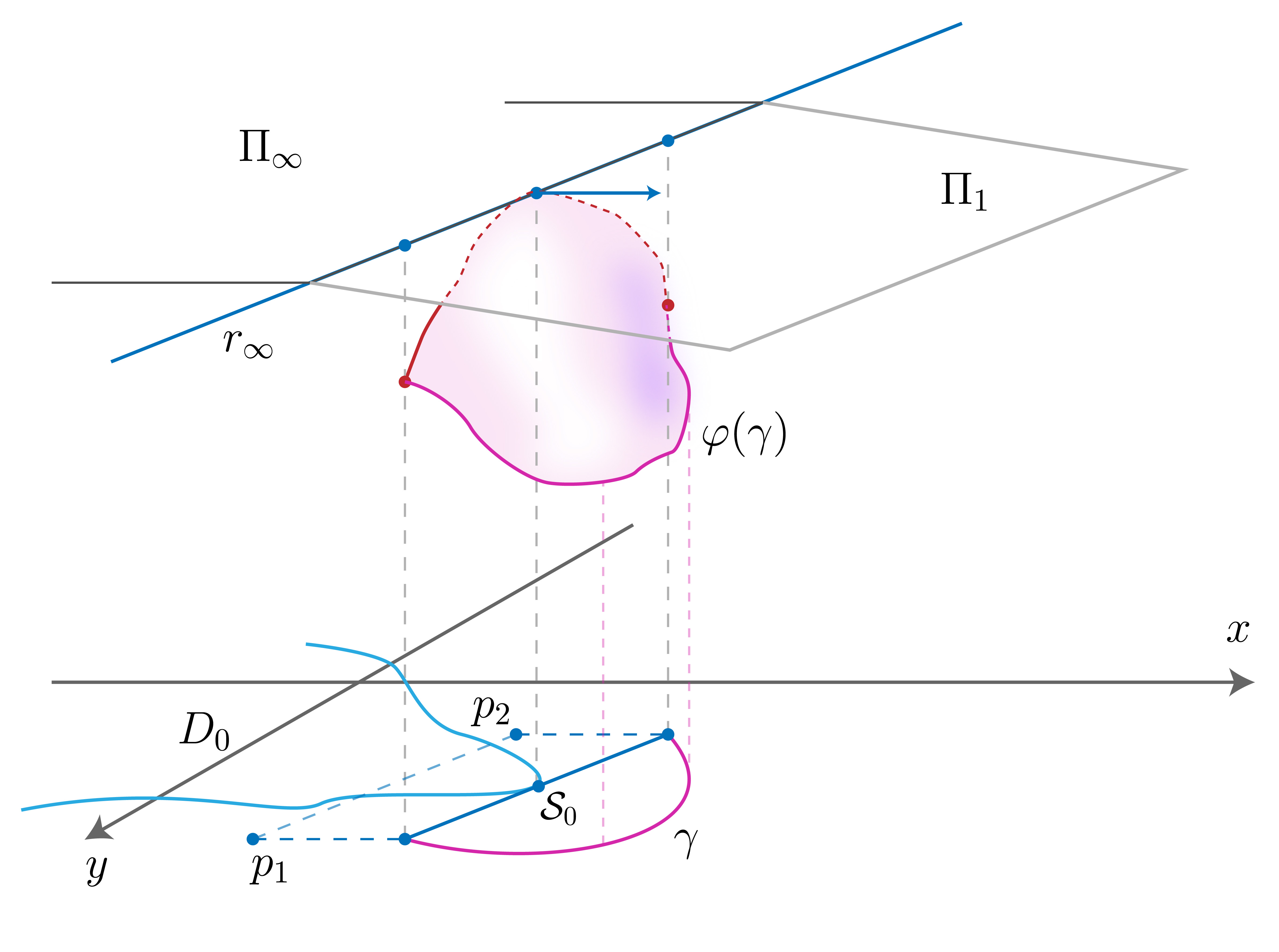
Figure 2.4. The argument in the proof of Assertion 2.8.

Consider next the graph $\mathcal{G}$ in $\mathbb{R}^{3}$ given by the restriction of $z=h(x,y)$ to the compact domain of $\mathbb{R}^{2}$ bounded by the segment $\mathcal{S}_{0}$ and the curve $\gamma$. Since $\mathcal{G}$ is saddle and its boundary does not touch the half-space of $\mathbb{R}^{3}$ above $\Pi_{1}$, then $\mathcal{G}$ also has this property. But now, observe that at the points of the non-empty set $\mathcal{S}_{0}\cap D_{0}$ we have $h_{x}=\mu_{\rm max}$. Since the slope of $\Pi_{1}$ in the $x$-direction is smaller than $\mu_{\rm max}$, this implies that there should exist points of $\mathcal{G}$ above $\Pi_{1}$, a contradiction. This proves Assertion 2.8. ∎

Since $D^{-}$, $D^{+}$ are disjoint, open convex sets of $\mathbb{R}^{2}$, there exists a line $\mathcal{L}\subset\mathbb{R}^{2}$ that separates them strictly, i.e., $D^{-}$ and $D^{+}$ lie in different connected components of $\mathbb{R}^{2}-\mathcal{L}$. In particular, any point of the straight half-line $\mathcal{L}^{*}:=\mathcal{L}\cap\{y\geq\delta_{0}\}$ lies in the set

(2.27) $$\mathcal{D}=\{(x,y):y\geq\delta_{0},x\in[x^{-}(y),x^{+}(y)]\}.$$

Observe that, by iii) of (2.26), we have $h_{x}=\mu_{\rm max}$ and $h=P_{\infty}$ on $\mathcal{D}$, i.e., $\varphi(\mathcal{D})\subset\Pi_{\infty}\cap\Sigma$. Since the intersection of $\nabla u(\mathbb{S}^{2})$ with the support plane $x=\mu_{\rm max}$ of $\mathbb{R}^{3}$ is just the point $p_{0}$, we deduce that $\psi(\mathcal{D})=\{p_{0}\}$, where $\psi$ is given by (2.14). Thus, $h_{y}$ is constant on $\mathcal{D}$. In particular, $h_{x}$ and $h_{y}$ are constant along $\mathcal{L}^{*}$, with $h_{x}=\mu_{\rm max}$. Then, $\varphi(\mathcal{L}^{*})$ is a straight half-line that lies in $\Sigma\cap\Pi_{\infty}$, and we deduce from there that $h_{y}=b_{\infty}$ on $\mathcal{D}$, where $b_{\infty}$ is defined in (2.25). In particular, the limit plane $\Pi_{\infty}$ is tangent to $\Sigma$ at every point of $\varphi(\mathcal{D})$. Also,

(2.28) $$p_{0}=(\mu_{\rm max},b_{\infty},*)\in\mathbb{R}^{3}.$$

Note that if $\delta_{0}=-\infty$, both $\mathcal{L}^{*}$ and $\varphi(\mathcal{L}^{*})$ are (complete) lines.

Step 8: Existence of a geodesic semicircle in $(\nabla u)^{-1}(p_{0})$.

In this step we show that, by choosing in a more careful way the initial direction $\nu_{0}\in(\nabla u)^{-1}(p_{0})$ that we fixed at the beginning of Step 3, we can ensure that $\Omega_{\xi}:=(\nabla u)^{-1}(p_{0})$ contains a geodesic semicircle of $\mathbb{S}^{2}$.

Assume that this last property is not true. Let $\beta$ be any geodesic arc of $\mathbb{S}^{2}$ contained in $\Omega_{\xi}$, and denote its endpoints by $\{\beta_{0}^{1},\beta_{0}^{2}\}$. Note that, by our choice of the direction $\xi$ in Step 3, the distance in $\mathbb{S}^{2}$ between the compact subsets $\Omega_{\xi}$ and $\{\xi,-\xi\}$ is positive (since $p_{0}$ is a Pogorelov point). Thus, we can consider the angle $\theta(\beta)\in[0,\pi]$ at $\xi$ defined by the two geodesic semicircles $\gamma_{1},\gamma_{2}$ of $\mathbb{S}^{2}$ with endpoints $\{\xi,-\xi\}$ that satisfy $\beta_{0}^{i}\in\gamma_{i}$. See Figure 2.5. Since $\beta$ has length $<\pi$ by hypothesis, this angle is $<\pi$.

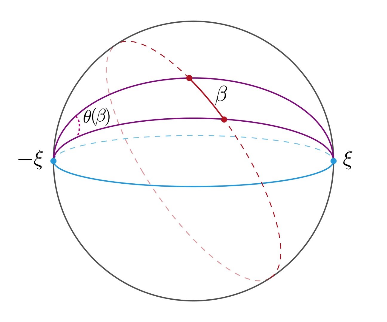
Figure 2.5. The definition of angle $\theta(\beta)$.

Observe first of all that there exists at least one geodesic arc (of positive length) $\beta^{*}$ contained in $\Omega_{\xi}$. To see this, let $\mathcal{L}^{*}$ denote the straight half-line of the $(x,y)$-plane whose existence was shown in Step 7. Let $\beta^{*}$ be the geodesic arc in $\mathbb{S}^{2}$ that corresponds to $\mathcal{L}^{*}$ via the totally geodesic bijection $\mathbb{R}^{2}\rightarrow\mathbb{S}^{2}_{+}$ given by (2.15). Since $h_{x}=\mu_{\rm max}$ along $\mathcal{L}^{*}$, we have from (2.14) and (2.28) that

(2.29) $$\beta^{*}\subset(\nabla u)^{-1}(p_{0})=\Omega_{\xi}.$$

Since $\mathcal{L}^{*}$ is not parallel to the $y$-axis, clearly $\theta(\beta^{*})>0$.

We next prove that there exists a geodesic arc $\beta_{\infty}$ of maximum angle in $\Omega_{\xi}$. Let $\theta_{0}\in(0,\pi]$ denote the supremum of the angles $\theta(\beta)$, among all possible choices of geodesic arcs $\beta$ contained in $\Omega_{\xi}$. Take any sequence of geodesic arcs $\{\beta_{n}\}_{n}$ in $\Omega_{\xi}$ with $\theta(\beta_{n})\to\theta_{0}$. Then, up to a subsequence, the endpoints $a_{n},b_{n}$ and the midpoint $c_{n}$ of the $\beta_{n}$ converge to three geodesically aligned points $\{a_{1},a_{2},a_{3}\}$ in $\Omega_{\xi}$. Since any point of $\beta_{n}$ is a convex combination of its endpoints, we deduce that $\{\beta_{n}\}_{n}$ converges to the geodesic arc $\beta_{\infty}$ contained in $\Omega_{\xi}$ with endpoints $\{a_{1},a_{2}\}$ and midpoint $a_{3}$. In particular, $\beta_{\infty}$ has positive length $<\pi$, and $\theta(\beta_{\infty})=\theta_{0}$. We then conclude that $\theta_{0}<\pi$.

Once we know this property, it is clear that we can choose the original $\nu_{0}\in(\nabla u)^{-1}(p_{0})$, which was initially chosen in Step 3 without any a priori limitation, as follows: $\nu_{0}$ is the unique point of the geodesic arc $\beta_{\infty}\subset\Omega_{\xi}$ with the property that the angles $\theta_{1},\theta_{2}$ of the two geodesic arcs of $\beta_{\infty}$ joining $\nu_{0}$ with each of the endpoints $\{a_{1},a_{2}\}$ of $\beta_{\infty}$ satisfy $\theta_{i}=\theta_{0}/2<\pi/2$, for $i=1,2$. See Figure 2.6.

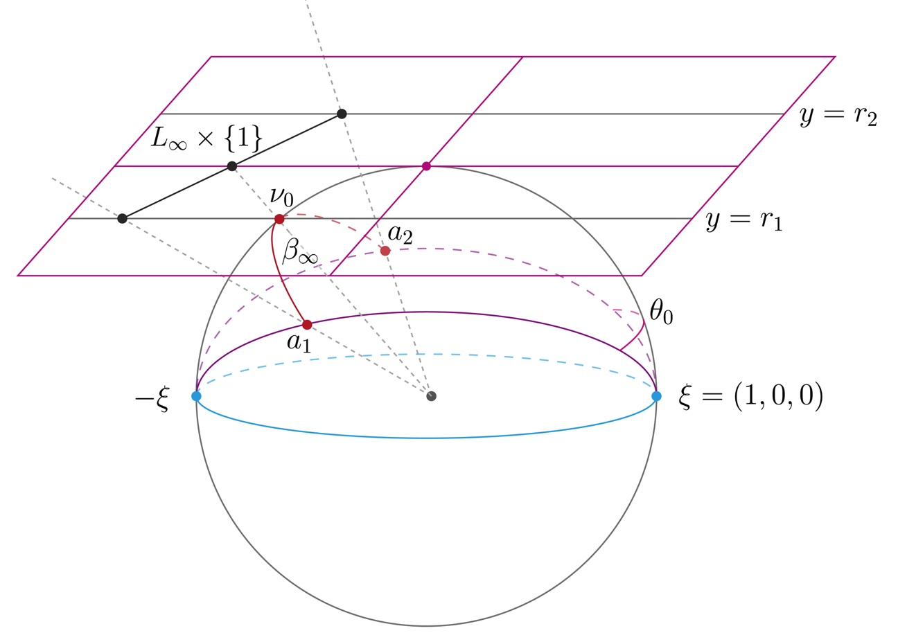
Figure 2.6. Choice of $\nu_{0}\in(\nabla u)^{-1}(p_{0})$.

This choice for $\nu_{0}$ lets us choose in a more specific way the coordinates $(x,y,z)$ at the beginning of Step 3. Recall that, in these $(x,y,z)$ coordinates, we had $\xi=(1,0,0)$, $\nu_{0}=(\nu_{0}^{1},0,\nu_{0}^{3})$ with $\nu_{0}^{3}>0$. By our new specific choice of $\nu_{0}$, after a suitable rotation of the $(x,y,z)$-coordinates around the $x$-axis, we can additionally suppose that the arc $\beta_{\infty}$ lies in the hemisphere $\mathbb{S}^{2}\cap\{z>0\}$. Note that $\nu_{0}\in\beta_{\infty}$, and that every point of $\beta_{\infty}$ lies in $(\nabla u)^{-1}(p_{0})$.

Consider the totally geodesic bijection $\mathbb{R}^{2}\rightarrow\mathbb{S}^{2}_{+}$ given by (2.15). This bijection takes $\nu_{0}$ to $(x_{0},0)$ for some $x_{0}\in\mathbb{R}$, and $\beta_{\infty}$ to a compact line segment $L_{\infty}$ passing through $(x_{0},0)$. See Figure 2.6. In the same way, the geodesic semicircles $\gamma_{1},\gamma_{2}$ in $\mathbb{S}^{2}\cap\{z\geq 0\}$ that pass through the points $\{\xi,-\xi,a_{i}\}$ are projected into two parallel lines in $\mathbb{R}^{2}$ of the form $y=r_{i}$, for some $r_{1}<0<r_{2}$. Obviously, each of the endpoints of $L_{\infty}$ lies in one of these lines.

We can now carry out the argument in Steps 3 through 7 for this new choice of $\nu_{0}$. Let $\mathcal{D}\subset\mathbb{R}^{2}\cap\{y\geq\delta_{0}\}$ denote the subset given by (2.27) in Step 7 of the proof. Since $\psi(L_{\infty})=\{p_{0}\}$, where $\psi$ is given by (2.14), we deduce from (2.28) that $(h_{x},h_{y})=(\mu_{\rm max},b_{\infty})$, constant along $L_{\infty}$. Also, observe that $(x_{0},0)\in\mathcal{D}\cap L_{\infty}$ and recall that $\varphi(\mathcal{D})\subset\Pi_{\infty}\cap\Sigma$. In this way, $\varphi(L_{\infty})\subset\Pi_{\infty}\cap\Sigma$. Since $h_{x}=\mu_{\rm max}$ along $L_{\infty}$, we conclude by the definition of $\delta_{0}$ that $\delta_{0}\leq r_{1}$.

Consider next the geodesic arc $\beta^{*}$ in (2.29). It corresponds via (2.15) to the half-line $\mathcal{L}^{*}=\mathcal{L}\cap\{y\geq\delta_{0}\}$. Since we have proved that $[r_{1},r_{2}]\subset[\delta_{0},\infty)$, this geodesic arc $\beta^{*}$ has angle $\theta(\beta^{*})$ greater than $\theta(\beta_{\infty})=\theta_{0}$. This is a contradiction with the definition of $\theta_{0}$. Therefore, $(\nabla u)^{-1}(p_{0})$ contains a geodesic semicircle of $\mathbb{S}^{2}$.

Step 9: Existence of a geodesic semicircle in $(\nabla u)^{-1}(p)$ for at least $4$ different points.

We have seen that, for any Pogorelov point $p_{0}\in\nabla u(\mathbb{S}^{2})$ of the hedgehog $\nabla u(\mathbb{S}^{2})$, the set $(\nabla u)^{-1}(p_{0})$ contains a geodesic semicircle. We will next show that there exist at least four different Pogorelov points for $\nabla u(\mathbb{S}^{2})$, what proves the statement above.

Let $p$ be a contact point of $\nabla u(\mathbb{S}^{2})$ with one of its support planes, and consider the set $\mathcal{N}_{p}:=\{\xi\in\mathbb{S}^{2}:p\in\Pi_{\xi}\}$. Note that the convex hull $\mathcal{C}$ of $\nabla u(\mathbb{S}^{2})$ is not contained in a plane, since $\nabla u$ has some regular point of negative curvature (see the proof of Assertion 2.3). In these conditions, it is well known that $\mathcal{N}_{p}$ is a compact, convex subset of an open hemisphere of $\mathbb{S}^{2}$.

Arguing by contradiction, assume that $\nabla u(\mathbb{S}^{2})$ has at most three (distinct) Pogorelov points $p_{1},p_{2},p_{3}$. Then $\mathcal{V}:=\mathbb{S}^{2}\setminus\cup_{i=1}^{3}\mathcal{N}_{p_{i}}$ is a non-empty open set, since each $\mathcal{N}_{p_{i}}$ lies in an open hemisphere. For almost any $\xi\in\mathcal{V}$, the intersection $\Pi_{\xi}\cap\nabla u(\mathbb{S}^{2})$ is a unique point $q_{\xi}$, which is not a Pogorelov point. Thus, from the definition of Pogorelov point, either $\nabla u(\xi)=q_{\xi}$, or $\nabla u(-\xi)=q_{\xi}$, for almost all $\xi\in\mathcal{V}$. If for any such $\xi_{0}$ it holds $\nabla u(-\xi_{0})\neq q_{\xi_{0}}$ , then, by definition of support plane,

$$\langle\nabla u(-\xi_{0})-q_{\xi_{0}},\xi_{0}\rangle<\langle\nabla u(\xi_{0})-q_{\xi_{0}},\xi_{0}\rangle=0,$$

and so

$$\langle\nabla u(-\xi_{0}),\xi_{0}\rangle<\langle\nabla u(\xi_{0}),\xi_{0}\rangle.$$

Hence, this property holds in a neighborhood $\mathcal{W}\subset\mathcal{V}$ of $\xi_{0}$, and it implies that for almost every $\xi\in\mathcal{W}$, we have $\nabla u(\xi)=q_{\xi}$. In particular, $\nabla u$ is singular in a neighborhood of $\xi_{0}$, since regular points of $\nabla u(\mathbb{S}^{2})$ never touch support planes. If $\nabla u(\xi_{0})\neq q_{\xi_{0}}$, the same argument gives that $\nabla u$ is singular in a neighborhood $\mathcal{W}$ of $-\xi_{0}$, and $\nabla u(\xi)=q_{-\xi}$ for almost every $\xi\in\mathcal{W}$.

Finally, if $\nabla u(\xi)=\nabla u(-\xi)=q_{\xi}$ for almost all $\xi\in\mathcal{V}$, we have that $\nabla u$ is singular in $\mathcal{V}$.

In other words, we have shown that there exists an open set $\mathcal{W}\subset\mathbb{S}^{2}$ such that $\nabla u$ is singular everywhere on $\mathcal{W}$, and for almost every $\xi\in\mathcal{W}$, we have that $\nabla u(\xi)$ is the unique contact point of $\nabla u(\mathbb{S}^{2})$ with one of the support planes $\Pi_{\xi}$ or $\Pi_{-\xi}$.

Recall that, by homogeneity, $D^{2}u$ always has a zero eigenvalue at every point, corresponding to the radial direction, and that the regular points of the hegdehog $\nabla u(\mathbb{S}^{2})$ are those where the rank of $D^{2}u$ is $2$; see the paragraph before Definition 2.2. Since $\nabla u$ is singular on $\mathcal{W}$, by reducing $\mathcal{W}$ if necessary, we can assume additionally that the rank of $D^{2}u$ is constantly equal to $0$ or $1$ in $\mathcal{W}$. We rule out these two cases separately.

Assertion 2.9.

The rank of $D^{2}u$ cannot be zero in $\mathcal{W}$.

Proof.

Assume that $D^{2}u=0$ in $\mathcal{W}$, and choose $\xi\in\mathcal{W}$. Suppose, for definiteness, that $\nabla u(\xi)=q_{\xi}\in\Pi_{\xi}$; the discussion is similar if $\nabla u(\xi)\in\Pi_{-\xi}$.

We will start arguing as in Step 3. Consider Euclidean coordinates $(x,y,z)$ in $\mathbb{R}^{3}$ such that $\xi=(1,0,0)$, and let $\Sigma$ be the entire saddle graph in $\mathbb{R}^{3}$ given by $z=h(x,y)$, where $h$ is defined by (2.1). Then, equations (2.17) and (2.18) at the beginning of Step 3 hold, but (2.19) does not. Since $u$ is linear in a neighborhood of $\xi$, with $u_{x}=\mu_{\rm max}$, we deduce that instead of (2.19) we have in our context that

(2.30) $$h_{x}(x,y)=\mu_{\rm max}~\hskip 28.45274pt\text{$\forall(x,y)\in(0,\infty)\times\mathbb{R}$ with $x^{2}\geq\delta(y^{2}+1),$}$$

for some $\delta>0$. In this way, if we choose $(x_{0},0)$ with $x_{0}>\delta$ and define the linear function

$$P(x,y):=\mu_{\rm max}(x-x_{0})+h_{y}(x_{0},0)y+h(x_{0},0),$$

we have that $h(x,y)=P(x,y)$ in a connected planar subset $\Omega\subset\mathbb{R}^{2}$ that contains the set defined in (2.30), and $h(x,y)>P(x,y)$ in $\mathbb{R}^{2}-\Omega$.

By the argument in Assertion 2.8, we deduce that $\mathbb{R}^{2}-\Omega$ is an open convex set. Consider the set $\Theta_{0}\subset\mathbb{S}^{2}$ given by the points $\nu$ of the form (2.15), with $(x,y)\in\Omega$. Since (2.15) is a totally geodesic mapping, this means that, if $\mathbb{S}_{+}^{2}:=\mathbb{S}^{2}\cap\{z>0\}$, then $\mathbb{S}_{+}^{2}\setminus\Theta_{0}$ is a convex set of $\mathbb{S}_{+}^{2}$. But now, note that the Euclidean coordinates $(x,y,z)$ were chosen arbitrarily except for the condition $\xi=(1,0,0)$. Thus, if we define $\Theta\subset\mathbb{S}^{2}$ as the set of points $\nu\in\mathbb{S}^{2}$ that are given by (2.15) for some $(x,y)\in\Omega$ with respect to some Euclidean coordinates $(x,y,z)$ with $\xi=(1,0,0)$, we deduce then that $\mathbb{S}^{2}\setminus\Theta$ is a convex set of $\mathbb{S}^{2}$, and $u$ is linear on $\Theta$. Then, $\mathbb{S}^{2}\setminus\Theta$ lies in an open hemisphere. Consequently, $u$ is linear on a closed hemisphere $H$ of $\mathbb{S}^{2}$, with $\nabla u=q_{\xi}$. Consider next the homogeneous function $v(p):=u(p)-\langle p,q_{\xi}\rangle$, defined for all $p\in\mathbb{R}^{3}$. Note that $D^{2}v=D^{2}u$ everywhere, and that $v$ vanishes along the geodesic $\partial H$ of $\mathbb{S}^{2}$. By [13, Thm. 1.6.4] or [8, Thm. 2], $v$ must be linear. Hence, $u$ is linear, a contradiction. ∎

Assertion 2.10.

The rank of $D^{2}u$ cannot be $1$ in $\mathcal{W}$.

Proof.

In order to prove the assertion, we use some results of hegdehog theory developed by Martinez-Maure in [10], that we explain next. Given $h\in C^{2}(\mathbb{S}^{2})$, let $\mathcal{H}$ be the hedgehog in $\mathbb{R}^{3}$ with support function $h$, i.e. $\mathcal{H}$ is given by

$$\chi(\nu):=\nabla_{\mathbb{S}}\,h(\nu)+h(\nu)\nu:\mathbb{S}^{2}\rightarrow\mathcal{H}\subset\mathbb{R}^{3},$$

where $\nabla_{\mathbb{S}}$ denote the gradient in $\mathbb{S}^{2}$. We assume that the curvature of $\chi$ is negative at its regular points, and that $\chi$ is not constant. Note that the hedgehog $\mathcal{H}:=\nabla u(\mathbb{S}^{2})$ of our problem is in these conditions.

For any $\omega\in\mathbb{S}^{2}$, consider the plane $P=\{\omega\}^{\perp}$, and let $\pi:\mathbb{R}^{3}\rightarrow P$ denote the orthogonal projection. Define $\chi_{\omega}:\mathbb{S}^{1}\equiv\mathbb{S}^{2}\cap P\rightarrow P$ by

(2.31) $$\chi_{\omega}(\theta):=\pi(\chi(\theta)).$$

Then, $\chi_{\omega}$ defines a planar hedgehog in $P$, that we denote by $\mathcal{H}_{\omega}=\chi_{\omega}(\mathbb{S}^{1})$. Since $\mathcal{H}$ has negative curvature at its regular points, this projected hedgehog $\mathcal{H}_{\omega}$ has empty convex interior; see Theorem 2 and Corollary 1 in [10], where the definition of convex interior of a planar hedgehog (which we will not use explicitly) is also presented; see also Corollary 1 in [11].

We now prove Assertion 2.10 using this information. Since $D^{2}u$ has rank one in the open set $\mathcal{W}\subset\mathbb{S}^{2}$, then $\nabla u(\mathcal{W})$ is a regular curve $\gamma$. Also, note that for almost every $q\in\gamma$ we have either $\{q\}=\Pi_{\xi}\cap\nabla u(\mathbb{S}^{2})$ or $\{q\}=\Pi_{-\xi}\cap\nabla u(\mathbb{S}^{2})$.

Let $T$ be the unit tangent vector to $\gamma$ at $q$, and define $\omega:=T\times\xi$. Let $\pi:\mathbb{R}^{3}\rightarrow\{\omega\}^{\perp}$ denote the orthogonal projection onto $P=\{\omega\}^{\perp}$. Then $\beta:=\pi(\gamma)$ is a regular curve in $P=\{\omega\}^{\perp}$ around $\pi(q)$, and $\pi(q)\in\beta\cap\mathcal{H}_{\omega}$ (since $\langle T,\omega\rangle=0$), where $\mathcal{H}_{\omega}$ is the planar hedgehog given by (2.31). Note that $\pi(q)$ is a regular point of $\mathcal{H}_{\omega}$, since $\chi_{\omega}(T)=\pi(q)$ and $\langle\nabla u(q),T\rangle\neq 0$, by regularity of $\gamma$. Also, either $\mathcal{H}_{\omega}$ lies on one side of the line $L_{\xi}=\Pi_{\xi}\cap P$, and in that case $\pi(q)\in L_{\xi}\cap\mathcal{H}_{\omega}$, or else $\mathcal{H}_{\omega}$ lies on one side of $L_{-\xi}=\Pi_{-\xi}\cap P$, and $\pi(q)\in L_{-\xi}\cap\mathcal{H}_{\omega}$. In this way, in any of these two cases, the planar hedgehog $\mathcal{H}_{\omega}\subset P$ touches one of its support lines at the regular point $\pi(q)$. Since $\mathcal{H}_{\omega}$ has empty convex interior, we obtain a contradiction with [10, Proposition 1]. ∎

Thus, we have proved that $\nabla u(\mathbb{S}^{2})$ has at least four Pogorelov points, as claimed.

Step 10: The final contradiction.

We now conclude the argument of the proof of Theorem 1.3. Recall that we had initially assumed that $u$ is not a linear function, and we were arguing by contradiction.

We have shown in Step 9 that there exist at least $4$ different points $p_{1},\dots,p_{4}\in\nabla u(\mathbb{S}^{2})$ for which $(\nabla u)^{-1}(p_{j})$ contains a geodesic semicircle $\Gamma_{j}$ of $\mathbb{S}^{2}$. The geodesic semicircles $\Gamma_{1},\dots,\Gamma_{4}$ are disjoint, since the $p_{j}$ are different.

Consider the region $\mathcal{O}\subset\mathbb{S}^{2}$ defined below (1.4). By hypothesis on $\mathcal{O}$, we have $\mathcal{O}\cap\Gamma_{j}\neq\emptyset$ for some $j\in\{1,\dots,4\}$. Let $\Omega_{j}$ denote the compact set $(\nabla u)^{-1}(p_{j})$. Thus, $\Omega_{j}\cap\mathcal{O}\neq\emptyset$ and, since $\mathcal{O}$ is connected, either $\partial\Omega_{j}\cap\mathcal{O}\neq\emptyset$ or $\mathcal{O}\subset\Omega_{j}$.

Suppose, in the first place, that $\mathcal{O}\subset\Omega_{j}$. Then, it is clear that the distance from $\mathcal{O}$ to any of the semicircles $\Gamma_{k}$, $k\neq j$, is positive. In particular, there exists $\varepsilon>0$ such that $\mathcal{O}$ does not intersect the open set $\mathcal{U}_{\varepsilon}:=\{\nu\in\mathbb{S}^{2}:{\rm dist}(\nu,\Gamma_{k})<\varepsilon\}$. But on the other hand, it is clear that there exist infinitely many closed disjoint geodesic semicircles contained in $\mathcal{U}_{\varepsilon}$. This contradicts the hypothesis that $\mathcal{O}$ intersects any configuration of $4$ disjoint geodesic semicircles. Thus, $\mathcal{O}$ is not contained in $\Omega_{j}$.

Hence, there must exist some $w_{j}\in\partial\Omega_{j}\cap\mathcal{O}$. Since $w_{j}\in(\nabla u)^{-1}(p_{j})$, we can choose $w_{j}$ as the vector $\nu_{0}\in\mathbb{S}^{2}$ in the argument that we carried out in Steps 3 through 7. Specifically, choose Euclidean coordinates $(x,y,z)$ so that $\xi_{j}=(1,0,0)$ and $w_{j}=:\nu_{0}=(\nu_{0}^{1},0,\nu_{0}^{3})$, with $\nu_{0}^{3}>0$. Denote $\mathbb{S}^{2}_{+}=\mathbb{S}^{2}\cap\{z>0\}$. Then, by the argument in Steps 3 through 7, the connected component of the set $(\nabla u)^{-1}(p_{j})\cap\mathbb{S}_{+}^{2}$ that contains $\nu_{0}$ is made of the points $\nu\in\mathbb{S}^{2}$ given by (2.15), with $(x,y)$ a point of the planar set $\mathcal{D}$ defined in (2.27). Also, (2.28) holds for $p_{0}:=p_{j}$.

Take $x_{0}\in\mathbb{R}$ given by $\nu_{0}=\frac{1}{\sqrt{1+x_{0}^{2}}}(x_{0},0,1)$. Since $\nu_{0}\in\partial\Omega_{j}$, obviously $(x_{0},0)\in\partial\mathcal{D}$, and $h_{x}(x_{0},0)=\mu_{\rm max}$ by (2.28) and (2.14). Thus, $h_{x}$ has an absolute maximum at $(x_{0},0)$. Hence, as $\nu_{0}:=w_{j}$ lies in $\mathcal{O}$, it follows by Assertion 2.1 that $h_{x}$ is constant around $(x_{0},0)$, since $\nabla h$ cannot be an open mapping. Then, by (2.14), $\nu_{0}$ lies in the interior of $\Omega_{j}$, a contradiction with $\nu_{0}\in\partial\Omega_{j}$.

By this final contradiction, the function $u$ must be linear, and this proves Theorem 1.3.

3.  Proof of Theorem 1.4

In Steps 2 through 9 of our proof of Theorem 1.3 we actually showed the following result. Let $u\in C^{2}(\mathbb{R}^{3}\setminus\{0\})$ be a degree one homogeneous solution to a linear equation (1.1). Assume that the coefficients $a_{ij}$ of (1.1) satisfy the degenerate ellipticity conditions (i), (ii) in (1.5). Let $\nabla u:\mathbb{S}^{2}\rightarrow\mathbb{R}^{3}$ be the restriction of the gradient of $u$ to $\mathbb{S}^{2}$. Then, there exist at least $4$ different points $p_{1},\dots,p_{4}$ in $\mathbb{R}^{3}$ such that each $(\nabla u)^{-1}(p_{j})$ contains a geodesic semicircle $\Gamma_{j}$, for $j=1,\dots,4$. These semicircles are disjoint, and $D^{2}u$ vanishes along the configuration $\Gamma=\cup_{i=1}^{4}\Gamma_{i}$.

As explained at the beginning of Step 2, there is an equivalence between degree one homogeneous solutions $u\in C^{2}(\mathbb{R}^{3}\setminus\{0\})$ of (1.1) whose coefficients satisfy conditions (i), (ii) in (1.5), and $C^{2}$ saddle functions $v(x)=u(x/|x|)$ on $\mathbb{S}^{2}$. Taking into account this equivalence, it is then clear that the result obtained in Steps 2 through 9 that we just recalled directly proves Theorem 1.4.

Theorem 1.4 is equivalent to the geometric statement below. Indeed, if $\rho\in C^{2}(\mathbb{S}^{2})$ denotes the support function of an ovaloid satisfying (3.1), then $v:=\rho-c$ is a saddle function in $\mathbb{S}^{2}$, thus in the conditions of Theorem 1.4 (and conversely).

Theorem 3.1.

Let $S\subset\mathbb{R}^{3}$ be a $C^{2}$ ovaloid in $\mathbb{R}^{3}$ whose principal curvatures $\kappa_{1},\kappa_{2}$ satisfy

(3.1) $$(\kappa_{1}-c)(\kappa_{2}-c)\leq 0$$

for some $c>0$. Then, $S$ is round along $4$ geodesic semicircles. Specifically, $S$ is tangent up to second order to four spheres $\Sigma_{1}^{c},\dots,\Sigma_{4}^{c}$ of radius $1/c$ along four disjoint geodesic semicircles $\alpha_{j}\subset\Sigma_{j}^{c}\cap S$, for $j=1,\dots,4.$

In other words, there exist $4$ disjoint geodesic semicircles $\Gamma_{1},\dots,\Gamma_{4}$ in $\mathbb{S}^{2}$ such that, if $\eta:S\rightarrow\mathbb{S}^{2}$ is the Gauss map of $S$, then each $\eta^{-1}(\Gamma_{j})=\alpha_{j}$ is made of umbilic points of $S$, and coincides with a geodesic semicircle of a sphere of radius $1/c$ in $\mathbb{R}^{3}$.

José A. Gálvez

Departamento de Geometría y Topología,
Instituto de Matemáticas IMAG,
Universidad de Granada (Spain).

e-mail: jagalvez@ugr.es

Pablo Mira

Departamento de Matemática Aplicada y Estadística,
Universidad Politécnica de Cartagena (Spain).

e-mail: pablo.mira@upct.es

This research has been financially supported by: Projects PID2020-118137GB-I00 and CEX2020-001105-M, funded by MCIN/AEI /10.13039/501100011033, and Junta de Andalucia grants no. A-FQM-139-UGR18 and P18-FR-4049

References

[1] A.D. Alexandrov, Sur les théorèmes d’unicité por
les surfaces fermèes, C.R. Dokl Acad. Sci. URSS22
(1939), 99–102.
[2] A.D. Alexandrov, Uniqueness theorems for surfaces
in the large, I, Vestnik Leningrad Univ.11 (1956),
5–17. (English translation: Amer. Math. Soc. Transl.21 (1962), 341–354).
[3] K. Astala, T. Iwaniec, G. Martin, Elliptic partial differential equations and quasiconformal mappings in the plane. Mathematical Series; No. 48. Princeton University Press, 2009.
[4] J.A. Gálvez, P. Mira, M.P. Tassi, A quasiconformal Hopf soap bubble theorem, preprint (2021).
[5] P. Guan, Z. Wang, X. Zhang, A proof of Alexandrov’s
uniqueness theorem for convex surfaces in , Ann. Inst. H.
Poincare Anal. Non Lineaire33 (2016), 329–336.
[6] Q. Han, N. Nadirashvili, Y. Yuan, Linearity of homogeneous order-one solutions to elliptic equations in dimension three, Comm. Pure Appl. Math.56 (2003), 425–432.
[7] T. Iwaniec, V. Sverák, On mappings with integrable dilatation, Proc. Amer. Math. Soc.118 (1993), 181–188.
[8] D. Koutroufiotis, On a conjectured characterization of the sphere, Math. Ann.205 (1973), 211–217.
[9] R. Langevin, G. Levitt, H. Rosenberg, Hérissons et multihérissons (enveloppes paramétrées par leur application de Gauss), Banach Center Publications 20 (1988), 245–253.
[10] Y. Martinez-Maure, Indice d’un hérisson: étude et applications, Publ. Math.44 (2000), 237–255.
[11] Y. Martinez-Maure, Contre-exemple à une caractérisation conjecturée de la sphère, C.R. Acad. Sci. Math.332 (2001), 41–44.
[12] C. Mooney, Minimizers of convex functionals with small degeneracy set, Calc. Var.59, 74 (2020).
[13] N. Nadirashvili, V. Tkachev, S. Vlädut, Nonlinear elliptic equations and nonassociative algebras, Mathematical Surveys and Monographs, vol. 200, American Mathematical Society, Providence, RI, 2014.
[14] N. Nadirashvili, S. Vlädut, Homogeneous solutions of fully nonlinear elliptic equations in four dimensions, Comm. Pure Appl. Math.66 (2013), 1653–1662.
[15] G. Panina, New counterexamples to A.D. Alexandrov’s hypothesis, Adv. Geom.5 (2005), 301–317.
[16] G. Panina, Isotopy problems for saddle surfaces, Eur. J. Comb.31 (2010), 1160–1170.
[17] A.V. Pogorelov, Solution of one of A.D. Aleksandrov’s problems (in
Russian), Doklady Akad. Nauk SSSR360 (1998), 317–319. Translation: Doklady Math.57 (1998), 398–399.
[18] C. Pucci, Un problema variazionale per i coefficienti di equazioni differenziali di tipo ellittico, Ann. Sc. Norm. Sup. Pisa16 (1962), 159–172.
[19] M.V. Safonov, Nonlinear elliptic equations of second order. Lecture Notes. University of Florence, Italy, 1991.