A Note on Simulation-Based Inference by Matching Random Features

Abstract

We can, and should, do statistical inference on simulation models by adjusting the parameters in the simulation so that the values of randomly chosen functions of the simulation output match the values of those some functions calculated on the data. Results from the “state-space reconstruction” or “geometry from a time series” literature in nonlinear dynamics indicate that just $2d+1$ such functions will typically suffice to identify a model with a $d$-dimensional parameter space. Results from the “random features” literature in machine learning suggest that using random functions of the data can be an efficient replacement for using optimal functions. In this preliminary, proof-of-concept note, I sketch some of the key results, and present numerical evidence about the new method’s properties. A separate, forthcoming manuscript will elaborate on theoretical and numerical details.

1 Introduction

For decades, scientists have increasingly expressed their ideas as generative, simulate-able models of complex processes; these models aim to capture both mechanisms at work in the world and also measurement processes. This is good science, but a statistical problem.

Even when the phenomenon being simulated is complex, and the model produces high-dimensional output, the underlying parameter space of the model will often have many fewer dimensions. (It is arguably just this compression that makes the models insightful.) As one example among many, the intricate spatial-network epidemic model of Chang et al. (2020) has just three adjustable parameters not fixed by direct measurement or background knowledge. The data, on the other hand, consists of daily time series over multiple cities and a period of months; it’s 630-dimensional. Similar pairings of high-dimensional data and complex but comparatively-few-parameter models are common in astronomy, climatology, economics, evolutionary biology, and ecology, among other fields. All the distributions these models produce can really be fitted into a low-dimensional space (three-dimensional, in the case of Chang et al. (2020)). Statistical analysis for such models should thus focus on parametric inference.

This, however, is where the problems start. It is very common for these models to be easy to simulate but hard to calculate with. They can be “run forward” to generate detailed simulated data sets at low computational cost, even for big models with many latent details that do not show up in the final data. By changing the parameters of the generative model, we change the distribution of simulated outcomes. But the mapping from parameters to distributions is complicated, and we can’t usually calculate the implied distribution. It is not feasible to find the probability of a particular outcome as a function of the parameters, i.e., it is not feasible to calculate the likelihood function. This rules out using classical statistical techniques (Bayesian or frequentist) which rely on the likelihood function.

When we try to connect our simulation models to our data, we want the simulations to match the data somehow, but it’s often unclear what aspects of the data the simulations should try to match, and what they should ignore as noise.

These three aspects of combining sophisticated models and rich data have made it clear we need methods for non-likelihood inference. Up to now, practitioners have pursued strategies where simulation models are tuned to match summary statistics or features calculated from the data. These summaries have been carefully crafted to ensure that (i) they are easily calculated from data; (ii) their expectation values change rapidly as the parameters of the simulation are adjusted; and (iii) any given value of the summary statistics implies a unique value of the parameters, and vice versa. There is typically only one summary statistic per parameter. Checking whether summary statistics have these three properties is usually a lot of work, and if one’s first attempt doesn’t meet the criteria, one has to start over and try something else.

This paper is about making simulation-based inference much simpler and more automatic. The goal is to replace the procedure of carefully selecting of a very small number of summary statistics, instead using about twice as many random functions of the data. Results in nonlinear dynamics say that “typical” smooth functions from a $d$-dimensional set (e.g., a 3-dimensional family of distributions) into a higher, $k$-dimensional space are smoothly invertible once $k>2d$, so that the values of $2d+1$ “typical” functions should be enough to identify $d$ parameters. Results from machine learning show that randomly selecting a small number of functions of a high-dimensional space can convey almost as much information as optimal summary statistics. Bringing these ideas together suggests we can estimate models with a (comparatively) small number of parameters from high-dimensional data, by matching a small number of random features of the data, without the step of carefully crafting summaries.

§2 gives a high-level overview of the idea of this paper, as well as fixing the necessary notation, and giving forward references to sections of the paper clarifying some aspects of the idea. §3 goes over the related work I’m drawing on, in simulation-based inference (§3.2), in the use of random features in machine learning (§3.3), and in embeddings in nonlinear dynamics and topology (§3.4); §3.1 recalls some general results about extremum estimators from asymptotic statistical theory for context. §4 sketches the theory, while §5 gives proof-of-concept numerical experiments.

2 Overview, Setting and Notation

You, the scientist, want to study a process in the world, which has produced a multi-dimensional data point $x_{n}$ in a sample space $\mathcal{X}_{n}$. (Here $n$ may be a sample size, duration of a time series, extent of a spatial field, etc.) You have a generative model of the process you think is at work, with some unknown parameters, $\theta\in\Theta\subset\mathbb{R}^{p}$. Each value of $\theta$ leads to a distribution $P_{n,\theta}$ over $\mathcal{X}_{n}$, with densities $p_{n,\theta}(x)$ (with respect to some convenient reference measure). You would like to estimate $\theta$, or test whether $\theta=\theta_{0}$, or quantify the uncertainty in $\theta$. When you ask me for help in doing this, my instinct as a statistician is to try to do all these things using the log-likelihood function. You then break the news that calculating $p_{n,\theta}(x)$ is intractable. But you can simulate the model easily, at whatever value of $\theta$ I ask for, giving me, say, $\tilde{X}(\theta)$.

The core idea of this paper is that I should now draw $k$ real-valued functions $F_{1},\ldots F_{k}$ at random from a distribution $D$ over a suitable class of functions $\mathcal{F}$, picking the functions independently of each other and of the data. Applying these functions to the observed $x_{n}$ gives a vector $F(x_{n})\in\mathbb{R}^{k}$. My random-feature estimate of $\theta$ would then be

$$\hat{\theta}=\operatorname*{argmin}_{\theta\in\mathbb{R}^{k}}{\frac{1}{2}\left\|F(x_{n})-P_{n,\theta}F\right\|^{2}}$$ (1)

Going forward, abbreviate $P_{n,\theta}F$ by $\Phi(\theta)$. Conditional on the choice of $F$, this is just an extremum estimator, so the usual theory of such estimators applies (see §3.1). In particular, if (i) $\Phi(\theta):\mathbb{R}^{d}\mapsto\mathbb{R}^{k}$ is smooth with a smooth inverse, and (ii) a concentration property holds, so that $F(X_{n})\rightarrow\Phi(\theta_{0})$ as $n\rightarrow\infty$, familiar arguments establish the consistency of $\hat{\theta}$. If the optimum in Eq. 1 is well-behaved (an interior minimum with non-singular Hessian, etc.), then conventional arguments establish asymptotic standard errors. If a central limit theorem holds for $F$, we get asymptotic Gaussianity.

Since we generally can’t calculate expectations exactly, $\Phi(\theta)$ may seem as un-available as the likelihood. But since you can simulate the model easily, $\Phi(\theta)$ can be approximated by $s^{-1}\sum_{r=1}^{s}{F(\tilde{X}^{(r)}(\theta))}$, where $r$ indexes independent runs of the model. An estimate based on such simulations will be a simulation-based random-feature estimate.

Readers familiar with the literature on simulation-based inference will have recognized this as akin to simulated minimum-distance estimators such as the “method of simulated generalized moments” and “indirect inference”, which also involve matching summary statistics (see §3.2). Craft lore among practitioners going back to the 1990s suggests that the summaries to be matched must be picked carefully, as the wrong features will be uninformative about $\theta$. If the features are chosen well, though, lore suggests that $k=d$ features are enough to get consistency, asymptotic normality, etc. The novelty in this paper lies in using precisely $k=2d+1$ features, drawn at random.

The idea that $2d+1$ features should be enough comes out of nonlinear dynamics, and ultimately topology. Simplifying (see §3.4), “embedding” a $d$-dimensional manifold $\Theta$ into $\mathbb{R}^{k}$ means finding a function $f:\Theta\mapsto\mathbb{R}^{k}$ which is smooth, invertible, and has a smooth inverse. It turns out that as soon as $k\geq 2d+1$, the “typical” $f$ is an embedding, so long as each coordinate of $f$ is a $C^{1}$ function and $\Theta$ is compact. Since $\Phi(\theta)$ is a map from $\Theta$ to $\mathbb{R}^{k}$ which we would like to be an embedding, $2d+1$ features should “typically” suffice. (§3.4 will explain the meaning of “typical” here.)

The idea that random features should be almost as informative as carefully-chosen features comes out of work on “replacing optimization with randomization” in machine learning (§3.3). A characteristic result in this literature, for instance, asserts that predictors of the form $\sum_{i=1}^{k}{\alpha_{i}F_{i}(x)}$, for $F_{i}$ drawn iidly from a fixed distribution over $\mathcal{F}$, will have nearly the same risk as predictors of the form $\int{\alpha(\omega)F(x;\omega)d\omega}$. Further, such random functions can themselves serve as function bases, with powerful approximation properties. These results work especially when the inputs $x$ are themselves high dimensional.

Bringing these results about random features together with the results on embedding suggests that using as few as $2d+1$ random features should be almost as good for estimation as even the optimal selection of features.

3 Background and Related Work

I will only highlight work which immediately inspired these ideas, or forms an obvious alternative approach.

3.1 The Usual Asymptotics

It will help to recall some well-established results about extremum estimators (as found in, e.g., Gouriéroux and Monfort (1989/1995, vol. I) or van der Vaart (1998, §§5.2 5.3, 5.6)). We have a sequence of random loss functions $M_{n}(\theta)$ (which are $X_{n}$-measurable). The estimator is $\hat{\theta}\equiv\operatorname*{argmin}_{\theta\in\Theta}{M_{n}(\theta)}$. Assume that as $n\rightarrow\infty$, $M_{n}(\theta)\rightarrow m(\theta)$, where the non-random limiting function $m$ has a unique minimum at the $\theta_{0}$ which generated the data. Further assume that $\theta_{0}$ is in the interior of $\Theta$, and that $M_{n}$ and $m$ are regular enough to allow whatever operations we need. Taylor-expanding the gradient $\nabla M_{n}(\hat{\theta})=0$ around $\theta_{0}$ yields a sandwich covariance matrix for $\hat{\theta}$:

$$\mathbb{V}\left[\hat{\theta}\right] \approx \left(\nabla\nabla m(\theta_{0})\right)^{-1}\mathbb{V}\left[\nabla M_{n}(\theta_{0})\right]\left(\nabla\nabla m(\theta_{0})\right)^{-1}$$ (2)

Gaussian fluctuations of $M_{n}$ around $m$ (for large $n$) will usually translate into Gaussian fluctuations of $\hat{\theta}$ around $\theta_{0}$.

Specialized to the situation of §2 above,

$$M_{n}(\theta) = \frac{1}{2}\|\Phi(\theta)-F(X_{n})\|^{2}$$ (3)

$$m(\theta) = \frac{1}{2}\|\Phi(\theta)-\Phi(\theta_{0})\|^{2}$$ (4)

and abbreviating

$$\mathbf{g} \equiv \nabla\Phi(\theta_{0})$$ (5)

$$v(n) \equiv \mathbb{V}\left[F(X_{n})\right]$$ (6)

we get

$$\nabla M_{n}(\theta_{0}) = (\Phi(\theta_{0})-F(X_{n}))^{T}\mathbf{g}$$ (7)

$$\mathbb{V}\left[\nabla M_{n}(\theta_{0})\right] = \mathbf{g}^{T}v(n)\mathbf{g}$$ (8)

$$\nabla\nabla m(\theta_{0}) = \mathbf{g}^{T}\mathbf{g}$$ (9)

$$\mathbb{V}\left[\hat{\theta}\right] \approx \left(\mathbf{g}^{T}\mathbf{g}\right)^{-1}\mathbf{g}^{T}v(n)\mathbf{g}\left(\mathbf{g}^{T}\mathbf{g}\right)^{-1}$$ (10)

The last result is conditional on the choice of random features $F$. All else being equal, then, the bigger $\mathbf{g}=\nabla\Phi(\theta_{0})$, the more precise our estimates will be. Of course, just multiplying the functions in $F$ by large constants won’t help, because that would scale up both the derivatives and the variances, canceling out exactly.

— I have used the ordinary (squared) Euclidean norm $\|F(X_{n})-\Phi(\theta)\|^{2}=(F(X_{n})-\Phi(\theta))^{T}(F(X_{n})-\Phi(\theta))$ for algebraic simplicty. We could instead use $(F(X_{n})-\Phi(\theta))^{T}\mathbf{w}(F(X_{n})-\Phi(\theta))$ for any symmetric, positive-definite $k\times k$ matrix $\mathbf{w}$, with the obvious change in asymptotic variances. Ideally, we’d use $\mathbf{w}=(\mathbb{V}\left[F(X_{n})\right])^{-1}$. This suggests a two-step estimation procedure, where we first use an unweighted norm (or one with a crude set of weights) to get an initial estimate $\tilde{\theta}$, then simulate from $\tilde{\theta}$ to approximate the variance matrix of the features and minimize the weighted norm to get a more precise estimate (Gouriéroux and Monfort, 1996).

A useful variant on this idea, due (so far as I know) to Wood (2010), is to act as though $F(X_{n})$ had a Gaussian distribution, with mean $\mu_{n}(\theta)=\Phi(\theta)$ and variance matrix $\mathbf{\Sigma}_{n}(\theta)$, and maximize the resulting likelihood. This may be approximately true if $F(X_{n})$ obeys a central limit theorem, and, even if not, serves to put more emphasis (as it were) on the dimensions of $F$ which should closely match $\Phi(\theta)$, and less emphasis on those dimensions of $F$ which are intrinsically noisier. I will refer to this idea as the use of a Wood likelihood, emphasizing that this is not the likelihood of the data, but an approximate likelihood for the features $F$.

3.2 Simulation-based inference

Many simulation modelers still make purely qualitative comparisons of simulation output to empirical data, essentially relying on a combination of theory and prior knowledge to constrain the form and parameters of models, plus the ability of experienced practitioners to (as it were) “smell out” mis-fits. Such qualitative approaches are sometimes quite structured and sophisticated (Windrum et al., 2007; O’Sullivan and Perry, 2013). But these approaches are, intrinsically, incapable of quantifying uncertainty.

Much of the impetus for frequentist simulation-based inference has come from econometrics (Gouriéroux and Monfort, 1996) and quantitative biology. Here the obstacles to using the likelihood arise partly from having many latent variables which would need to be integrated over (as emphasized by Gouriéroux and Monfort 1996), and, especially in biology, from the sensitive dependence of the dynamics on initial conditions (emphasized by Wood 2010). One response is to approximate the likelihood by doing density estimates on simulations, a strategy which is still being elaborated on (Cranmer et al., 2020) but faces basic curse-of-dimensionality issues.

My focus here is instead on likelihood-free strategies for simulation-based estimation. As mentioned above, the core idea shared by most such strategies is to pick some summary statistics, and then tune the $\theta$ parameters until summaries calculated on simulations match summaries calculated on the data. Methods differ, largely, in the nature of the summary statistics.

In symbols, the common idea begins with $k$ real-valued functions of the data, $f_{1},\ldots f_{k}$, collectively $f:\mathcal{X}_{n}\mapsto\mathbb{R}^{k}$. This induces a mapping $\phi:\Theta\mapsto\mathbb{R}^{k}$ by $\phi(\theta)=P_{n,\theta}f$. The ideal estimator would then be

$$\operatorname*{argmin}_{\theta\in\Theta}{\frac{1}{2}\|f(X_{n})-\phi(\theta)\|^{2}}$$ (11)

perhaps replacing the squared Euclidean norm with a weighted version as mentioned above. Consistency requires $f(X_{n})\rightarrow\phi(\theta_{0})$ as $n\rightarrow\infty$. This would lead to the asymptotic variance given by Eq. 10 above.

The “simulation-based” part comes from replacing the unavailable expectations with Monte Carlo approximations:

$$\hat{\theta}=\operatorname*{argmin}_{\theta\in\Theta}{\frac{1}{2}\|f(X_{n})-\overline{f}(\theta,n,s)\|^{2}}$$ (12)

where

$$\overline{f}(\theta,n,s)=\frac{1}{s}\sum_{r=1}^{s}{f(\tilde{X}^{(r)}_{n}(\theta))}$$ (13)

i.e., an average of $f$ over $s$ independent simulations of the model with the parameter set to $\theta$. Consistency requires that if $X_{n}\sim P_{n,\theta}$, then $f(X_{n})\rightarrow\phi(\theta)$ as $n\rightarrow\infty$. Under such an assumption, using $\overline{f}(\theta,n,s)$ instead of $\phi(\theta)$ inflates the variance of $\hat{\theta}$ by a factor of $1+1/s$ compared to Eq. 10. Alternately, just simulate from $\hat{\theta}$, repeat the estimation on the simulation outputs, and take the variance of the re-estimates.

3.2.1 The Method of Simulated (Generalized) Moments

seems to have been the first instance of this general scheme (McFadden, 1989; Lee and Ingram, 1991). The goal, unsurprisingly, was to approximate the celebrated “generalized method of moments” of Hansen (1982), where each $f_{i}$ function is itself an average over suitable units (time points, spatial locations, experimental subjects, etc.). Making the $f_{i}$s be averages means that laws of large numbers or ergodic theorems can be used to prove the convergence $f(X_{n})\rightarrow\phi(\theta_{0})$. Selecting the right generalized moments usually involves either detailed inspection of the model, or treating each coordinate of $X_{n}$ as a “moment”.

3.2.2 Indirect Inference (II)

arose when Gouriéroux et al. (1993); Smith (1993) moved away from relying on Hansen-style “generalized moments”. Rather, II introduces an “auxiliary” model, parameterized by, say, $\beta$, which is itself estimated by minimizing its own loss function. It is this estimate of $\beta$ which plays the role of $F(X_{n})$, and as usual $\theta$ is adjusted to minimize the distance between $F(X_{n})$ and $\overline{F}(\theta,n,s)$, the average estimate of $\beta$ from $s$ runs of the simulation with parameter $\theta$. (Using $s$ simulation per parameter value inflates the variance of the indirect-inference estimator by a factor of $1+1/s$ as before.) Consistency requires that $F(X_{n})\rightarrow b(\theta_{0})$ and $\overline{F}(\theta,n,s)\rightarrow b(\theta)$, for some non-random and invertible “binding function” $b(\theta)$, along with some minor regularity conditions Beginning in econometrics where it is still widely used (Halbleib et al., 2018), indirect inference has spread to ecology (Wood, 2010; Kendall et al., 2005) and even sociology (Ciampaglia, 2013).

The auxiliary models used in indirect inference need to be easily estimable, and sensitive enough to the $\theta$ parameters that $b(\theta)$ is invertible; ideally a smooth mapping with a smooth inverse. For time series, linear-Gaussian autoregressive or vector autoregressive models are often used (e.g., DeJong and Dave 2007); for spatial data, linear-Gaussian conditional autoregressive models. However, efficient estimation often involves a lot of work to devise informative auxiliary models; the closer the auxiliary model is to being well-specified, the more efficient indirect inference estimates will be. Nickl and Pötscher (2010) provided an elegant way around this, by making the auxiliary model a nonparametric density estimate based on the method of sieves. Unfortunately, their results presume that the generative model produces IID data, and it is far from clear how to generalize their intricate construction to dependent data, which is where simulation-based inference is most needed. Carrella et al. (2020) ingeniously suggested selecting and weighting summary statistics (including auxiliary parameter estimates) by simulating the model at a many random values of $\theta$, calculating a large suite of candidate auxiliaries, and then doing a regularized linear regression of $\theta$ on the candidate. While this may be faster than explicit optimization, it begs the question of where good summaries come from in the first place. It also (implicitly) uses a linear approximation to the inverse binding function $b^{-1}(\beta)$, which will usually be quite nonlinear.

3.2.3 Approximate Bayesian Computation (ABC)

is a related but distinct strategy for simulation-based inference, especially widely used in evolutionary biology and ecology (Beaumont, 2010) and epidemiology (Britton and Pardoux, 2019, §4.3). ABC tries to approximate the Bayesian posterior distributions $\pi(\theta|x_{n})$. The basic form goes as follows. Pick a (generally vector-valued) summary statistic $f$, as before, and a “tolerance” $\delta$. Find the empirical value of the summary, $f(x_{n})$. Now draw a $\theta$ at random from the prior $\pi(\theta)$; simulate $\tilde{X}(\theta)$ from the selected $\theta$; calculate $f(\tilde{X}(\theta))$. If $\|f(\tilde{X}(\theta))-f(x_{n})\|\leq\delta$, accept the $\theta$ and add it to the posterior sample, otherwise, discard it; repeat. The collection of accepted samples then approximates the posterior $\pi(\theta|x_{n})$. More precisely, it approximates $\pi(\theta|f(x_{n}))$, which will induce some distortions unless $f$ is a sufficient statistic for $\theta$. Further distortion is induced by the use of the tolerance $\delta$. Popular in practice, ABC’s theoretical properties are an on-going object of study (e.g., Frazier et al. 2018).

Again, the choice of summary statistics $f$ is usually seen as crucial. Attempts at automated choice of summary statistics, such as Barnes et al. (2012), have usually aimed to pick the most-nearly-sufficient statistic (or combination of statistics) from a pre-defined menu. Fearnhead and Prangle (2012) showed how to get good summary statistics from a knowledge of the posterior $\pi(\theta|x_{n})$ — which is what ABC is supposed to find. Vespe (2014, 2016) gave a more nearly constructive procedure by drawing values of $\theta$ from the prior, simulating $x$ from each $\theta$, and then using diffusion maps (Coifman and Lafon, 2006) to embed the $(\theta,x)$ pairs in a common space; the leading eigenfunctions of the diffusion operator provided the summary features. Because this is fundamentally a kernel-based approach, it may be possible to connect it to the random features results described below (§3.3).

3.3 Random Features in Machine Learning

Inspired largely by Rahimi and Recht (2008a), researchers in machine learning have explored the uses of randomly selected “features”, i.e., functions of the data, for prediction and other statistical tasks. Originally this was seen as a way to approximate kernel-based predictors. That is, the goal was to approximate predictors of the form $\sum_{i=1}^{n}{\beta_{i}K(x,x_{i})}$, with $K(\cdot,\cdot):\mathcal{X}\times\mathcal{X}\mapsto\mathbb{R}$ being the kernel function, with predictors of the form $\sum_{j=1}^{p}{\alpha_{j}f(x;\omega_{j})}$, with the $\omega_{j}$ being sampled from some suitable distribution over a function space $\mathcal{F}$ related to the kernel. In particular, the positive-definite properties of kernels suggested using the (normalized) Fourier transform of $K$ as a distribution over trigonometric functions and sampling from it, leading to random Fourier features. Beyond making kernel methods more practical for large computational problems, random Fourier features have been employed to measure dependence between random variables (Lopez-Paz et al., 2013), test statistical independence (Zhang et al., 2018) and conditional independence (Strobl et al., 2018), do two-sample testing (Sutherland and Schneider, 2015, §3.3), etc. Experience, and some theoretical results (e.g., Honorio and Li 2017) suggest that these methods can work especially well when the data space $\mathcal{X}$ is high dimensional. Other sets of random features, not based on Fourier transforms, have recently been advocated for tasks such as goodness-of-fit testing and evaluating the quality of Monte Carlo output (Huggins and Mackey, 2018). While I am don’t know of any results which directly use random features in this way for simulation-based inference, Briol et al. (2019) study simulation-based inference by minimizing the maximum mean discrepancy, a kernel-based discrepancy measure whose random-feature approximation is studied by e.g. Sutherland and Schneider (2015).

Going beyond the viewpoint of approximating kernels, however, Rahimi and Recht (2009, 2008b) developed powerful results on the strength of random features as function bases in their own right. Omitting minor regularity condition, Rahimi and Recht (2009) established that if we draw functions $F_{1},\ldots F_{K}$ iidly from a space $\mathcal{F}$ and fit a predictor of the form $\sum_{i=1}^{k}{\alpha_{i}F_{i}(x)}$ to training data, its excess risk compared to the optimal predictor of the form $\int_{\mathcal{F}}{\alpha(f)f(x)df}$ is $O(1/\sqrt{k})$ with high probability. Or, again, Rahimi and Recht (2008b) shows that an arbitrary integral mixture over $\mathcal{F}$ can be uniformly approximated to $O(1/\sqrt{k})$ using $k$ random functions from $\mathcal{F}$; furthermore, such integral mixtures are dense in a reproducing kernel Hilbert space. Thus for instance random Fourier features allow us to approximate every function in the RKHS induced by the Gaussian kernel, an extremely rich space.

From a different direction, Kulhavý (1996, pp. 115–117, pp. 123–125) outlined an approach to constructing sufficient statistics for $d$-parameter exponential families by applying $d$ different linear functionals to the log-likelihood function; provided the functionals are (linearly) independent, the result is, in fact, a sufficient statistic in 1-1 correspondence with the canonical sufficient statistic. For example, one can pick $d+1$ points in the parameter space, say $\theta_{0},\ldots\theta_{d}$, and take the $d$ log density ratios $\log{p_{n,\theta_{i}}(x)}-\log{p_{n,\theta_{0}}(x)}$ as the sufficient statistics, provided these functions are linearly independent of each other, which will generally be the case for random $\theta$s. The result needs the model to be an exponential family, or enveloped within an exponential family, so it doesn’t hold for most interesting simulation models, but it illustrates how a small number of random features can be highly informative about parametric families.

3.4 “Embedology”

Beginning with Packard et al. (1980), researchers in nonlinear dynamics pursued a program of “attractor reconstruction” or “geometry from a time series”, as follows. We observe a one-dimensional signal $y(t)$ which is a function $r(s(t))$ of some higher-dimensional state $s(t)$. We assume $s(t)$ evolves according to a smooth, deterministic dynamical system, so $s(t)=\rho_{t}(s(0))$ for a suitable semi-group of smooth functions $\rho_{t}$ (i.e., $\rho_{t+h}=\rho_{t}\circ\rho_{h}=\rho_{h}\circ\rho_{t}$). The attractor of this dynamic is a set $\mathcal{A}$. Since $s(t)$ is unobserved, we form the “time-delay vector” $u(t)=(y(t),y(t-\tau),\ldots y(t-(k-1)\tau)$ for some choice of delay $\tau$ and number of lags $k$. It is unsurprising that $y(t+\tau)$ can be predicted approximately from $u(t)$, especially for large $k$. What was surprising was that, in the “typical” or “generic” situation, there is a finite $k$ above which $u(t+\tau)=\psi_{\tau}(u(t))$ for a deterministic function $\psi_{\tau}$, which will also fix $y(t+\tau)$, More exactly, not only is there a differentiable mapping $\phi:\mathcal{A}\mapsto\mathbb{R}^{k}$ which takes $s(t)$ into $u(t)$, but this mapping has a differentiable inverse, and $\psi_{h}=\phi\circ\rho_{h}\circ\phi^{-1}$. The time-delay-embedding space of $u(t)$s is thus equivalent, “up to a smooth change of coordinates”, to the underlying state space of $s(t)$s — typically.

The mathematical basis for this is a classic result in differential geometry, the Whitney (1936) embedding theorem . This tells us that once $k\geq 2d+1$, the set of “embeddings” (differentiable, invertible maps with differentiable inverses) forms an open, dense set in the set of $C^{1}$ functions from the $d$-dimensional manifold $\mathcal{A}$ into $\mathbb{R}^{k}$. Embeddings are thus “generic” in the sense in which that word is used in topology. The extension of this result to dynamical systems, the Takens (1981) theorem, rested on showing this was still true when the coordinate functions of the mapping took the form $r\circ\rho_{\tau}$, for generic choices of $\rho$, $r$ and $\tau$. This was the foundation for a large body of applied work in nonlinear dynamics, as well as attempts to refine the underlying embedding theorem. Abarbanel (1996); Kantz and Schreiber (2004) review both theory and applications.

For our purposes, the most useful paper from this field was Sauer et al. (1991). This complemented the topological notion of “typicality” used by Whitney, Takens, etc., with a more probabilistic one. What one wants to say is that “almost every” map is an embedding, but this needs the intricate construction of a measure on an infinite-dimensional space. Sauer et al. (Theorem 2.2) finessed this by say that maps are “prevalent”: given any smooth map $f:\mathcal{A}\mapsto\mathbb{R}^{k}$, $k\geq 2d+1$, the perturbation $f+e$ is an embedding for Lebesgue-almost-all maps $e$ in a finite-dimensional subspace $E$. (If $\mathcal{A}$ is a subset of $\mathbb{R}^{l}$, we can take $E$ to be the $l(2d+1)$-dimensional space of linear functions.) This also implies that embeddings are dense among the smooth mappings.

3.5 Summary of Objectives

To sum up, the goal here is to establish that when we have a $d$-parameter generative model, we should be able to estimate the $d$ parameters by matching $k=O(d)$ functions, chosen independently from each other and from the data, drawn from a space of functions which is both rich enough to include “typical” smooth functions, and regular enough that sample values converge on expectations. The hope is that using randomly chosen functions will be (nearly) as efficient as using optimally chosen functions, and a further hope is that we can get consistency, and maybe even near efficiency, with just $k=2d+1$.

4 Theory

The two main goals of this note are to introduce the idea of doing simulation-based inference by matching random features, and to show that the concept is feasible by means of numerical experiments. A full exploration of the theory is reserved for a separate manuscript in preparation. Nonetheless, it is worth making a few remarks.

Throughout, I will employ the following notation:

• The parameters of the model live in $\Theta$.

• For each $\theta\in\Theta$ and $n\in\mathbb{N}$, $P_{n,\theta}$ is a probability measure on the sample space $\mathcal{X}_{n}$. The family of probability measures so induced will be $\mathcal{P}_{n}$.

I will also make the following assumptions.

1. $\Theta$ is a compact subset of $\mathbb{R}^{d}$.

2. The parameterization is non-redundant: if $\theta_{1}\neq\theta_{2}$, then $P_{n,\theta_{1}}\neq P_{n,\theta_{2}}$. (Actually this only needs to hold for all sufficiently large $n$.)

3. For each $n$, the collection of probability measures $\mathcal{P}_{n}$ is a statistical manifold in the sense of Amari et al. (1987); Kass and Vos (1997). In particular, if $\theta_{m}\rightarrow\theta$, then $P_{n,\theta_{m}}\rightarrow P_{n,\theta}$ in distribution, and vice versa.

4.1 Identifiability, Fisher-consistency and Consistency

Let’s say that a functional, e.g., is a real-valued function of a probability distribution, $\mathcal{P}_{n}\mapsto\mathbb{R}$. Because, under these assumptions, there is a smooth, 1-1 correspondence between the manifold of probability measures and the parameter space, I will abuse notation a little and also write $\Theta\mapsto\mathbb{R}$. If we could work at this level, that of functionals of probability measures / functions of the parameters, there’d be little difficulty. For $i\in 1:k$, say $\phi_{i}(\theta):\Theta\mapsto\mathbb{R}$ are our $k$ distinct functionals, and $\phi(\theta):\Theta\mapsto\mathbb{R}^{k}$ is the vector-valued functional we get by applying them all at once (in parallel!). Suppose that the individual $\phi_{i}$ are $C^{1}$ in the parameters. Then the embedding theorems (§3.4) tell us that, for large enough $k$, embeddings are an open, dense set in this space of functions, and that Lebesgue-almost-all perturbations of non-embeddings are embeddings. If we just observed $\phi(P_{n,(}\theta_{0}))$, we could invert $\phi$ to recover $\theta_{0}$. That is, Fisher-consistency would be typical, once we used enough functionals which were $C^{1}$ in the parameters.

Lemma 1

Assume all the things. Let $\mathcal{M}$ be the collection of smooth, real-valued functionals on $\mathcal{P}_{n}$. By composition, for any $m\in\mathcal{M}$, we may define a smooth function on $\Theta$. Let $\mu$ be a collection of $2d+1$ such functions, so $\mu:\Theta\mapsto\mathbb{R}^{2d+1}$. Then the set of $\mu$ which form embeddings of $\Theta$ in $\mathbb{R}^{2d+1}$ is an open, dense set, and embeddings are prevalent.

Proof: Direct application of theorems 2.1 (genericity) and 2.2 (prevalence) in Sauer et al. (1991). $\Box$

For better or for worse, we don’t get to work with functions of the parameters. We do not even really get to work with functionals of the probability measures, since we only have samples from those measures. The lemma is thus of little direct use. In order to make it useful, we need to relate it to measurable functions of the data, i.e., to statistics.

Now, under the assumptions above, in particular under the statistical-manifold assumption, as $\theta_{m}\rightarrow\theta$, then $P_{n,\theta_{m}}\rightarrow P_{n,\theta}$ weakly or in distribution. This in turn means that for any bounded, continuous test function $f:\mathcal{X}_{n}\mapsto\mathbb{R}$, $P_{n,\theta_{m}}f\rightarrow P_{n,\theta}f$. In fast, the topology of weak convergence is generated by neighborhoods of the form

$$\left\{P\in\mathcal{P}_{n}~{}:~{}|Pf-r|\leq\delta\right\}$$

varying $f$ over all bounded, continuous functions on $\mathcal{X}_{n}$, $r$ over $\mathbb{R}$, and $\delta$ over $(0,\infty)$ (Dembo and Zeitouni, 1998, p. 260). That is, the generating sets of the topology are ones where the expectation values of bounded, continuous test functions are close to target values. It follows that smooth functionals on this manifold are either the expectations of bounded, continuous test functions, or are the limits of sequences of such expectations. We thus have

Lemma 2

Assume all the things. Let $C_{b}$ be the collection of bounded, continuous functions on $\mathcal{X}_{n}$. Let $f$ be a collection of $k$ functions from $C_{b}$, and define $\phi_{i}:\Theta\mapsto\mathbb{R}$ via $\phi_{i}(\theta)=P_{n,\theta}f_{i}$, and $\phi:\Theta\mapsto\mathbb{R}^{k}$ similarly. Then the set of $\phi$ which are embeddings of $\Theta$ in $\mathbb{R}^{k}$ is an open, dense set, and embeddings are prevalent, once $k\geq 2d+1$.

Proof: By the statistical-manifold assumption, each $\phi_{i}$ is a $C^{1}$ function from $\Theta$ to $\mathbb{R}$. Moreover, as discussed above, the statistical manifold assumption also says that functions of this form are dense in the space of $C^{1}$ functions of the parameters. Now invoke the previous lemma. $\Box$.

Having whittled down from needing to get generic functionals of the distribution to just generic expectations of bounded, continuous test functions, it would be nice to say something about smaller classes of test functions.

Theorem 1

Assume all the things. Let $\mathcal{F}\subset C_{b}$ be a class of bounded, continuous functions on $\mathcal{X}_{n}$, and suppose that linear combinations from $\mathcal{F}$ are dense in $C_{b}$. Let $f$ be a collection of $k$ functions from $\mathcal{F}$, and define $\phi_{i}$ and $\phi$ as in the previous lemma. Then the set of $\phi$ which are embeddings of $\Theta$ in $\mathbb{R}^{k}$ is an open, dense set, and embeddings are prevalent, once $k\geq 2d+1$.

Sketch: This basically follows from the fact that the linear span of $\mathcal{F}$ is, under these assumptions, weak-convergence-determining (Ethier and Kurtz, 1986, p. 155), and the previous lemma.

Notice that the random Fourier features have a very natural role here, as convergence-determining class of bounded, continuous test functions.

The previous result is about what could be identified if we could work with expectation values of generic continuous, bounded statistics. Of course we can’t do that; we have only a single realization of the underlying process. To make the transition from data to distributions, we need to ensure that $f(X_{1:n})\rightarrow P_{n,\theta_{0}}f$ as $n\rightarrow\infty$, for all $f\in\mathcal{F}$. The typical requirements for such a concentration property are (i) some sort of Lipschitz condition, so that $f(X_{1:n})$ doesn’t depend too much on any one coordinate of $X_{1:n}$, and (ii) some weak dependence conditions on the model (Kontorovich and Raginsky, 2017). This is basically all that’s needed; if the (idealized or infeasible) estimator $\operatorname*{argmin}_{\theta}{\|f(X_{n})-P_{n,\theta}f\|}$ would be consistent, then as a routine corollary the simulation-based estimator $\operatorname*{argmin}{\|f(X_{n})-\overline{f}(\theta,n,s)]\|}$ will also be consistent, with the variance increased by a factor of $1+1/s$ (p. 13).

4.2 Testing

The whole previous development has focused on point estimation and its uncertainty, but these ideas also apply to hypothesis testing and model checking. Testing the hypothesis that $\theta=\theta_{0}$ is as simple as seeing whether $F(X_{n})$ is acceptably close to $\Phi(\theta_{0})$, with “acceptably close” being determined by simulating from $\theta_{0}$. Drawing additional independent functions from $\mathcal{F}$, beyond those used to estimate $\theta$, allows for goodness-of-fit. (Cf. Gelman and Shalizi 2013 on simulation-based model checking.) If we have a central limit theorem for the summary statistics, it would be possible to supplement simulation-based tests with an asymptotic $\chi^{2}$ test.

5 Numerical Experiments

The proof-of-concept is in the ability to actually run, so in this section, I report some numerical experiments on random-feature-matching estimates for some benchmark problems.

All numerical experiments were conducted using R, version 3.6.2 (R Core Team, 2015). The R file which generated all the figures and numerical results reported here is available on request, though there are legal restraints on commercial use of the code.

Throughout this section, I work with models which generate univariate sequences or time series. Experiments on higher-dimensional time series, and on spatial and spatio-temporal processes, will be reported elsewhere.

I rely on random Fourier features, of the form

$$F_{i}(X_{1:n})\equiv\frac{1}{n}\sum_{t=1}^{n}{\cos{(\Omega_{i}X_{t}+\alpha_{i})}}$$ (14)

or

$$F_{i}(X_{1:n})\equiv\frac{1}{n-1}\sum_{t=1}^{n-1}{\cos{(\Omega_{i}^{(1)}X_{t}+\Omega_{i}^{(2)}X_{t+1}+\alpha_{i})}}$$ (15)

Throughout, frequencies $\Omega\sim\mathcal{N}(0,1)$, and phases $\alpha$ were uniformly distributed on $(-\pi,\pi)$. Random linear transformations were generated using the expandFunctions package (Miller, 2016).

The “univariate” random Fourier features of Eq. 14 can be seen as empirical counterparts to the characteristic function for the marginal distribution of the $X_{t}$, evaluated at the random frequencies $\Omega_{1},\ldots\Omega_{k}$ (and with random phase shifts). The “bivariate” random Fourier features of Eq. 15 play the same role for the characteristic function of the marginal distribution of the pairs $(X_{t},X_{t+1})$. Because characteristic functions do, in fact, characterize probability distributions (Kallenberg, 2002, Thm. 5.3, pp. 84–87), the expectation values of these features are good candidates for generic functionals. Because these features also time- or sample- averages, their sample values will converge on expectations for a very broad range of data-generating processes. Again, further numerical experiments, using other random features, will be reported elsewhere.

— It would be natural to ask how random-feature estimates, in these examples, compare to previous approaches to simulation-based inference. Unfortunately, this is not as straightforward as one would wish. In the absence of truly off-the-shelf implementations of those other techniques, I would have to craft my own for each example. But then there would always be the possibility that (say) my implementation of indirect inference lost the race because I picked a bad auxiliary model for some example. The results of such comparisons will, nonetheless, be reported elsewhere.

Because the objective function can be rather spiky (particularly for the chaotic dynamical systems), they were optimized using generalized simulated annealing, as implemented in the GenSA package (Xiang et al., 2013). I limited each optimization to five seconds of computing time; some tinkering (not included here) showed great improvements in going from $0.5$ to $2$ seconds, and again from $2$ seconds to $5$ seconds, but little improvement from $5$ to $10$ seconds. I have made no further effort to find the most computationally-efficient way to minimize these objective functions.

5.1 IID Process and Univariate Random Features

5.1.1 Gaussian Location Family

I begin with the simplest possible baseline case, estimating the location $\mu\in\mathbb{R}$ of an IID univariate Gaussian $\mathcal{N}(\mu,1)$. I begin by checking that three ($=2d+1$) random Fourier features are, in fact, not only enough to uniquely identify $\mu$, but that the mapping is smoothly invertible. Figure 1 shows that, indeed, it is, and that sample-to-sample variation in the features is already quite negligible at $n=100$.

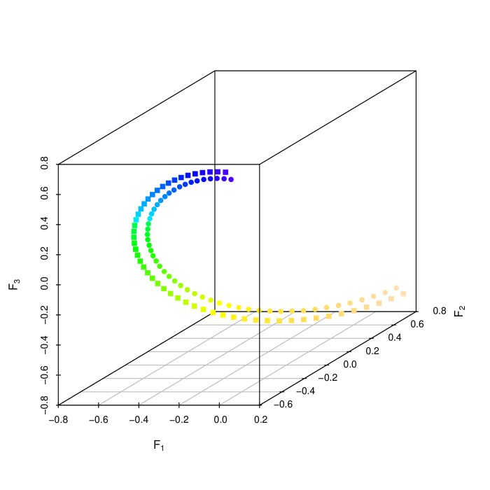
Figure 1: Using 3 random univariate Fourier features on the model $N(\theta,1)$, $n=100$, with feature values from 2 separate random realizations shown in two separate plotting symbols; color denotes $\theta$. Note: This is using the “French” approach of using the parameters to transform a fix set of random draws, rather than re-randomizing at each parameter value.

Figure 2: Numerical evaluation of the distance between one sample of a standard Gaussian distribution ($\mathcal{N}(0,1)$), and unit-variance Gaussian distributions with varying means $\mu$. The distance was evaluated using $10$ random draws per value of $\theta$, and using the same three random Fourier features used for the preceding plots.

The efficient way to estimate $\mu$ is, of course, just to use the sample mean, which is the MLE. The distribution of this estimator will be $\mathcal{N}(\mu,1/n)$, and the MSE will be $1/n$. Random feature matching will not do better than this, but the question is how close it will come. Figure 3 shows that we do, in fact, come rather close, at least in this rather simple setting.

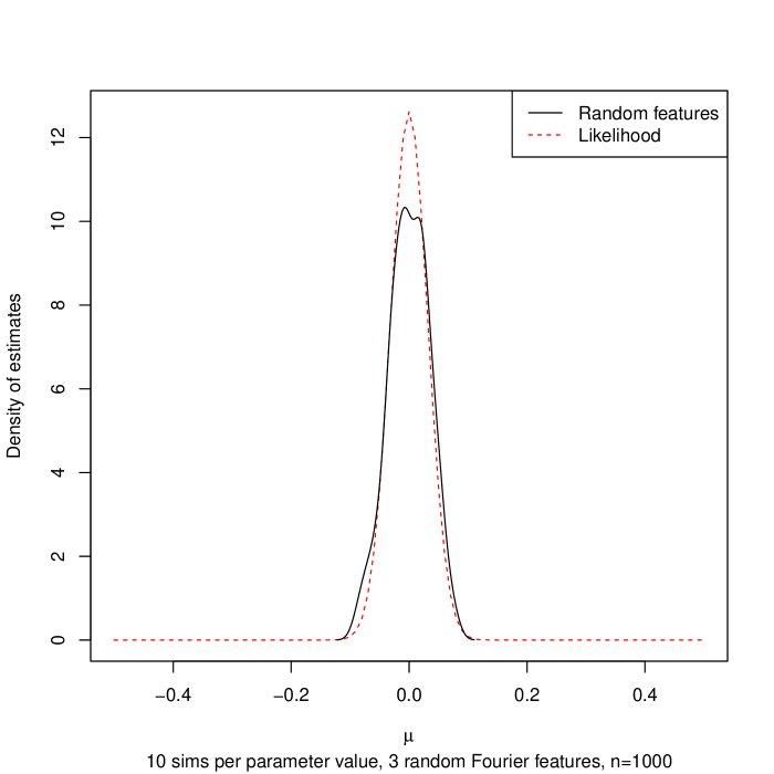
Figure 3: Density of random-feature estimates (kernel-smoothed) versus the (theoretical) density of the MLE, when estimating the location of a univariate Gaussian by minimizing the distance with 3 random Fourier features.

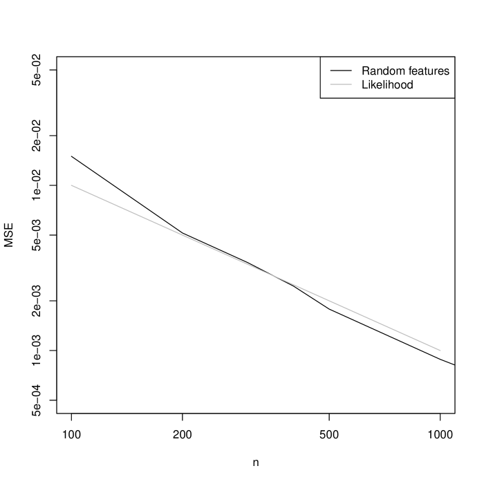
Figure 4: MSE of estimating the location parameter of a univariate Gaussian (i.e., $\mu$ in $N(\mu,1)$ family) with 3 random Fourier features and 10 simulations for each parameter value considered during the optimization. The true $\mu$ is fixed at 0 as the sample size is varied (with 100 replicates at each sample size. The grey line shows the theoretical MSE of the maximum likelihood estimate, which here is just $\sigma^{2}/n=1/n$.

5.1.2 $t$-Distribution Location Family

The Gaussian distribution is of course the simplest possible test-case for estimation. A natural next step is to consider another location family. Specifically, I consider the family where $X=\mu+T$, where $T$ is a standard $t$-distributed random variable with 5 degrees of freedom. This is heavy tailed (fifth and higher moments are ill-defined), but still a one-parameter family where the distribution changes smoothly with the parameter.

Using the same three random Fourier features as in the Gaussian example still manifestly gives an embedding (Figure 5). Minimizing distance in those features gives estimates which are not much worse than the MLE (Figure 6).

Figure 5: Numerical evaluation of the distance between one sample of a centered $t$ distribution ($n=300$, $df=5$), and $t$ distributions with the same number of degrees of freedom centered at $\theta$. The distance was evaluated using $10$ random draws per value of $\theta$, and using the same three random Fourier features used for the Gaussian location examples earlier.

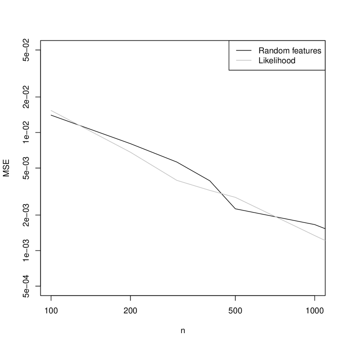
Figure 6: MSEs for estimating the location parameter of a $t$-distribution with 5 degrees of freedom, using distance-minimization on the same 3 random Fourier features as used for the Gaussian, and for the MLE (evaluated numerically, using the fitdistr function from the MASS library (Venables and Ripley, 2002)). Results are averages over 100 trials, with 10 simulations per considered parameter value.

5.1.3 Estimating a Dynamical Systems from Its Invariant Distribution

We don’t actually need the machinery of simulation-based inference to estimate the location parameters of bell curves, even heavy-tailed ones. I thus turn to a much more challenging example, namely the logistic map, a deterministic dynamical system defined by

$$S_{t+1}=4rS_{t}(1-S_{t})$$ (16)

where both the state variable $S_{t}\in[0,1]$, and the dynamical parameter $r$ are $\in[0,1]$. The observable, above $X_{n}$, will be the whole sequence or trajectory $(S_{1},S_{2},\ldots S_{n})$, so $\mathcal{X}_{n}=[0,1]^{n}$.

For small values of $r$, the sole fixed point is $S=0$ and every trajectory approaches it, so the only invariant distribution is the point mass at 0. Otherwise, every $r$ has its own invariant distribution over $[0,1]$ (Figure 7). If $S_{1}$ is drawn from this invariant distribution, then the trajectory $S_{1},S_{2},\ldots$ is the realization of a stationary, and indeed ergodic, Markov process, and every $r$ has a unique natural ergodic distribution over trajectories. (Even if $S\sim\mathrm{Unif}(0,1)$, the trajectory very quickly approaches stationarity.) For sufficiently large values of $r$, the system may be chaotic, meaning that it is both ergodic and shows sensitive dependence on initial conditions. One such parameter value is $r=0.9$, which is what will be used in the experiments below, though the behavior of the estimation method at other parameter values is quite similar, whether or not the dynamics are chaotic.

Note that in this case, it’s hard to see how we could use the method of maximum likelihood as a baseline. Since $S_{1}$ is observed, for a particular $r$, the trajectory $(S_{1},S_{2},\ldots S_{n})$ is either impossible (likelihood 0) or mandatory (likelihood 1). While it’s true that the correct $r$ will uniquely maximize this likelihood, actually doing the optimization would be challenging to say the least. (Alternatively, of course, the ratio $\frac{S_{2}}{S_{1}(1-S_{1})}$ is enough to determine $r$ exactly.) Various ad hoc modifications are of course possible (e.g., saying we only observe whether or not each $S_{t}$ is in a bin of some narrow width), but it seems better to just admit that this is a domain where the method of maximum likelihood fails us.

As before, I will begin by showing that the values of 3 ($=2d+1$) random Fourier features will uniquely and smoothly identify the parameter $r$. Figure 8 does this using the same three features previously used in the IID location examples, to emphasize that we need to understand very, very little about the underlying model’s behavior in order to pick adequate features.

Figure 7: A (partial) display of the invariant distribution of the logistic map as a function of $r$. (It’s only partial because the distribution within the vertical bands is non-uniform.) The tick on the horizontal axis at $r=0.9$ indicates the true value of the parameter used in the estimation experiments that follow, though additional simulations (not shown) show very similar behavior for other values of $r$.

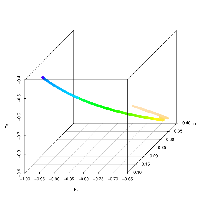
Figure 8: Values of the same univariate Fourier features used for the Gaussian example, evaluated along random trajectories of the logistic map, as a function of the logistic map parameter $r$. Features are evaluated by averaging 10 trajectories of length 100 each, with initial conditions chosen randomly in $[0,1]$. (Strictly speaking, then, these are not stationary time series.)

Figure 9: Density of random-feature matching estimates (kernel-smoothed) for the parameter $r$ of the logistic map from time series of length 100 and 10 simulations per parameter value, minimizing distance with respect to the same three univariate Fourier used for the location-family examples above. The true parameter was $r=0.9$ for all trials. The “data” trajectory was randomly regenerated for each of the 100 simulation trials, but the random features were kept constant. (Additional experiments, not included here, show that randomly regenerating the features for each trial broadens the distribution only slightly.) Note that subsequent figures will zoom in on the horizontal axis.

5.1.4 Estimating a Dynamical Systems from Bivariate Distributions

While, as mentioned, all large-enough values of $r$ lead to distinct invariant distributions over $[0,1]$, there is clearly some loss of information in going from whole trajectories to univariate random features. Using bivariate random Fourier features (as defined above) seems like a natural compromise, particularly if the models we’re entertaining are deterministic dynamical systems.

Again, numerically there is indeed an embedding using three random bivariate Fourier features (Figure 10). That being the case, I turn to estimation.

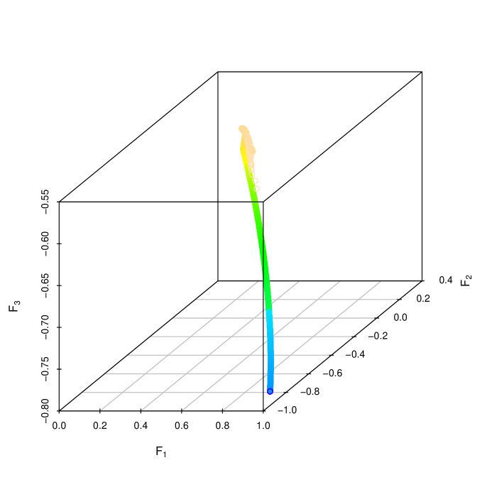
Figure 10: Identifiability of the logistic map parameter from bivariate random Fourier features, but otherwise as in Figure 8.

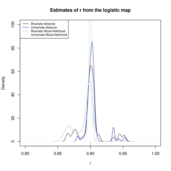
Figure 11: Distribution of estimates for the logistic map parameter value using 3 bivariate (black) and univariate (grey) random Fourier features, and $s=10$ simulations per parameter value in optimization. All time series are of length $100$, and the true parameter value, $0.9$, is marked by a tick on the axis. (The Wood likelihood estimates using univariate features are very concentrated around $r=0.9$, and so the vertical scale of this plot is truncated to show the shape of the other distributions.)

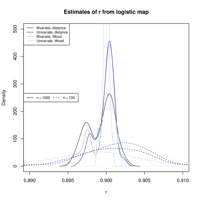
Figure 12: Distribution of estimates of $r$ from the logistic map (kernel-smoothed), comparing univariate vs. bivariate features, simple distance minimization vs. maximizing the Wood likelihood, and two sample sizes, all as in Figure 11. Notice that, compared to that figure, the horizontal axis has been zoomed in around the true parameter value $r=0.9$, and, again, the vertical axis cuts off the density of the most-concentrated estimator.

5.2 Logistic Map Observed Through Noise

So far, I have only dealt with one-parameter families, though the logistic map is a rather tricky one. To show that random-feature-matching doesn’t just work because of some quirk of one-dimensional families, I will now consider a two parameter family, which is actually a hidden Markov model, namely the logistic map observed through Gaussian noise. Specifically, the model specification is

$$S_{t+1}|S_{t} = 4rS_{t}(1-S_{t})$$ (17)

$$Y_{t}|S_{t} \sim \mathcal{N}(S_{t},\sigma^{2})$$ (18)

with only $Y_{t}$ being observable, so $X_{n}=(Y_{1},Y_{2},\ldots Y_{n})$. That is, in the hidden layer, $S_{t}$ follows the deterministic logistic map, but we do not get to see it face to face, but only through the distortion of additive Gaussian noise of variance $\sigma^{2}$. There are thus two parameters to estimate, $r$ and $\sigma^{2}$, so we require 5 random features.

Because I despair of making a five-dimensional plot, I will skip the visual display of embedding, and just go straight to reporting distributions of estimates (Figures 13 and 14). Unsurprisingly, estimates of $r$ are less precise, at equal sample sizes, than in the noise-free case, but the estimates are also, visibly, converging on the correct parameter values.

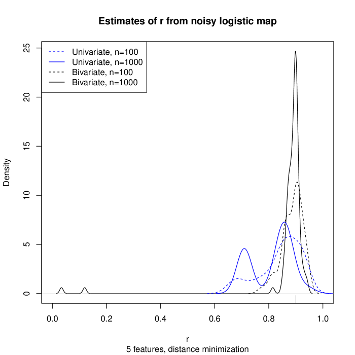
Figure 13: Density of estimates of $r$ from the noisy logistic map (kernel smoothed), showing univariate vs. bivariate features (blue vs. black) and $n=100$ vs. $n=1000$ (solid vs. dashed lines). 10 simulations were used per parameter value when optimizing. The true parameter value was held fixed at $r=0.9$.

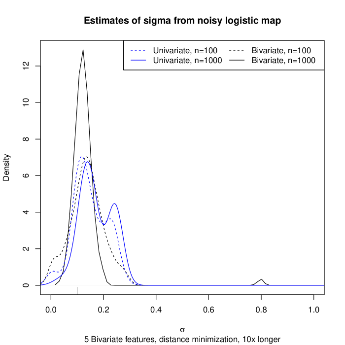
Figure 14: As in Figure 13, but for estimates of $\sigma$ (not $\sigma^{2})$; the true parameter value was held fixed at $\sigma=0.1$.

5.3 Notes on These Experiments

The last sub-section, on the logistic map seen through noise, shows that we can get quite good estimates using univariate and bivariate random Fourier features on a hidden Markov model. (This indicates that random feature matching doesn’t just work on Markov processes.) It is natural to wonder whether the choice of univariate, bivariate, or higher-order features could be automated. Information-theoretic (Marton and Shields, 1994; Steif, 1997) and learning-theoretic (McDonald, 2017) results on estimating joint distributions both suggest that with $n$ observations, it is feasible to non-parametrically estimate the distribution of blocks of whose length scales like $\log{n}$, but no faster. Of course we are dealing with parametric families of distributions, so a faster rate of block-growth with $n$ may be feasible, but $\log{n}$ should be safe.

These experiments have also been limited to stationary models Suitable choices of random features for non-stationary processes, which do not prejudge the form of the non-stationarity, will be reported elsewhere.

6 Summary

The argument of this manuscript is that when we want to do simulation-based inference on a model with $d$ parameters, we will generally be able to do so using $2d+1$ random nonlinear features, i.e., functions of the data, chosen independently of the data, and indeed of the model. The theory sketched above suggests that these features should come from a class of functions whose linear combinations are dense in the space of bounded, continuous test functions on the sample space. They should also be functions whose sample- or time- averages converge (rapidly) on expectation values. Random Fourier features therefore suggest themselves, but are by no means required. The numerical experiments reported above show that matching random features can be competitive, statistically, with maximum likelihood, and delivers good results in some situations where likelihood-based inference is scarcely feasible.

A more detailed treatment of the many theoretical and implementation questions raised by these preliminary results is in preparation. In the meanwhile, these results suggest that simulation-based inference can be made (much more nearly) automatic through matching random features, at little statistical cost.

Acknowledgments

A. E. Owen offered invaluable moral and intellectual support, and soundly vetoed multiple bad names for the technique. I wish to acknowledge the grant review panel which rejected a proposal based on this idea, thereby providing crucial motivation.

References

- Abarbanel (1996) Abarbanel, Henry D. I. (1996). Analysis of Observed Chaotic Data. Berlin: Springer-Verlag.
- Amari et al. (1987) Amari, Shun-ichi, O. E. Barndorff-Nielsen, Robert E. Kass, Steffen L. Lauritzen and C. R. Rao (1987). Differential Geometry in Statistical Inference, vol. 10 of Institute of Mathematical Statistics Lecture Notes-Monographs Series. Hayward, California: Institute of Mathematical Statistics. URL http://projecteuclid.org/euclid.lnms/1215467056.
- Barnes et al. (2012) Barnes, Chris, Sarah Filippi, Michael P.H. Stumpf and Thomas Thorne (2012). “Considerate Approaches to Achieving Sufficiency for ABC Model Selection.” Statistics and Computing, 22: 1181–1197. URL https://arxiv.org/abs/1106.6281. doi:10.1007/s11222-012-9335-7.
- Beaumont (2010) Beaumont, Mark A. (2010). “Approximate Bayesian Computation in Evolution and Ecology.” Annual Review of Ecology, Evolution, and Systematics, 41: 379–406. doi:10.1146/annurev-ecolsys-102209-144621.
- Briol et al. (2019) Briol, Francois-Xavier, Alessandro Barp, Andrew B. Duncan and Mark Girolami (2019). “Statistical Inference for Generative Models with Maximum Mean Discrepancy.” E-print, arxiv.org:1906.05944. URL https://arxiv.org/abs/1906.05944.
- Britton and Pardoux (2019) Britton, Tom and Etienne Pardoux (eds.) (2019). Stochastic Epidemic Models with Inference, Cham, Switzerland. Springer Nature Switzerland AG. doi:10.1007/978-3-030-30900-8.
- Carrella et al. (2020) Carrella, Ernesto, Richard M. Bailey and Jens Koed Madsen (2020). “Indirect inference through prediction.” Journal of Artificial Societies and Social Simulation, 23(1). URL https://arxiv.org/abs/1807.01579. doi:10.18564/jasss.4150.
- Chang et al. (2020) Chang, Serina, Emma Pierson, Pang Wei Koh, Jaline Gerardin, Beth Redbird, David Grusky and Jure Leskovec (2020). “Mobility Network Models of COVID-19 Explain Inequities and Inform Reopening.” Nature, 589: 82–87. doi:10.1038/s41586-020-2923-3.
- Ciampaglia (2013) Ciampaglia, Giovanni Luca (2013). “A Framework for the Calibration of Social Simulation Models.” Advances in Complex Systems, 16. URL https://arxiv.org/abs/1305.3842. doi:10.1142/S0219525913500306.
- Coifman and Lafon (2006) Coifman, Ronald R. and Stéphane Lafon (2006). “Diffusion Maps.” Applied and Computational Harmonic Analysis, 21: 5–30. doi:10.1016/j.acha.2006.04.006.
- Cranmer et al. (2020) Cranmer, Kyle, Johann Brehmer and Gilles Louppe (2020). “The frontier of simulation-based inference.” Proceedings of the National Academy of Sciences (USA), 117: 30055–30062. URL https://arxiv.org/abs/1911.01429. doi:10.1073/pnas.1912789117.
- Dalmasso et al. (2020) Dalmasso, Niccolò, Rafael Izbicki and Ann B. Lee (2020). “Confidence Sets and Hypothesis Testing in a Likelihood-Free Inference Setting.” In Proceedings of the 37th International Conference on Machine Learning [ICML 2020], pp. 2323–2334. URL https://arxiv.org/abs/2002.10399.
- DeJong and Dave (2007) DeJong, David N. and Chetan Dave (2007). Structural Macroeconometrics. Princeton, New Jersey: Princeton University Press.
- Dembo and Zeitouni (1998) Dembo, Amir and Ofer Zeitouni (1998). Large Deviations Techniques and Applications. New York: Springer Verlag, 2nd edn.
- Devaney (1992) Devaney, Robert L. (1992). A First Course in Chaotic Dynamical Systems: Theory and Experiment. Reading, Massachusetts: Addison-Wesley.
- Dynkin (1951) Dynkin, E. B. (1951). “Necessary and sufficient statistics for a family of probability distributions.” Uspekhi Matematicheskikh Nauk, 6: 68–90. In Russian.
- Ethier and Kurtz (1986) Ethier, Stewart N. and Thomas G. Kurtz (1986). Markov Processes: Characterization and Convergence. New York: Wiley.
- Fearnhead and Prangle (2012) Fearnhead, Paul and Dennis Prangle (2012). “Constructing Summary Statistics for Approximate Bayesian Computation: Semi‐automatic Approximate Bayesian Computation.” Journal of the Royal Statistical Society B, 74: 419–474. doi:10.1111/j.1467-9868.2011.01010.x.
- Frazier et al. (2018) Frazier, David T., Gael M. Martin, Christian P. Robert and Judith Rousseau (2018). “Asymptotic Properties of Approximate Bayesian Computation.” Biometrika, 105: 593–607. URL https://arxiv.org/abs/1607.06903. doi:10.1093/biomet/asy027.
- Gelman and Shalizi (2013) Gelman, Andrew and Cosma Rohilla Shalizi (2013). “Philosophy and the Practice of Bayesian Statistics.” British Journal of Mathematical and Statistical Psychology, 66: 8–38. URL http://arxiv.org/abs/1006.3868. doi:10.1111/j.2044-8317.2011.02037.x.
- Gouriéroux and Monfort (1989/1995) Gouriéroux, Christian and Alain Monfort (1989/1995). Statistics and Econometric Models. Themes in Modern Econometrics. Cambridge, England: Cambridge University Press. Translated by Quang Vuong from Statistique et modèles économétriques, Paris: Économica.
- Gouriéroux and Monfort (1996) — (1996). Simulation-Based Econometric Methods. Oxford, England: Oxford University Pres.
- Gouriéroux et al. (1993) Gouriéroux, Christian, Alain Monfort and E. Renault (1993). “Indirect Inference.” Journal of Applied Econometrics, 8: S85–S118. URL http://www.jstor.org/stable/2285076.
- Gray (1988) Gray, Robert M. (1988). Probability, Random Processes, and Ergodic Properties. New York: Springer-Verlag. URL http://ee.stanford.edu/~gray/arp.html.
- Halbleib et al. (2018) Halbleib, Roxana, Dennis Kristensen, Eric Renault and David Veredas (eds.) (2018). Indirect Estimation Methods in Finance and Economics, London. Elsevier. doi:10.1016/j.jeconom.2018.03.002. Special issue of the Journal of Econometrics (volume 205, issue 1).
- Hansen (1982) Hansen, Lars Peter (1982). “Large Sample Properties of Generalized Method of Moments Estimators.” Econometrica, 50: 1029–1054. URL https://www.jstor.org/stable/1912775. doi:10.2307/1912775.
- Honorio and Li (2017) Honorio, Jean and Yu-Jun Li (2017). “The Error Probability of Random Fourier Features is Dimensionality Independent.” URL https://arxiv.org/abs/1710.09953.
- Huggins and Mackey (2018) Huggins, Jonathan H. and Lester Mackey (2018). “Random Feature Stein Discrepancies.” In Advances in Neural Information Processing Systems 31 [NeurIPS 2018] (S. Bengio and H. Wallach and H. Larochelle and K. Grauman and N. Cesa-Bianchi and R. Garnett, eds.), pp. 1899–1909. Red Hook, New York: Curran Associates. URL https://arxiv.org/abs/1806.07788.
- Kallenberg (2002) Kallenberg, Olav (2002). Foundations of Modern Probability. New York: Springer-Verlag, 2nd edn.
- Kantz and Schreiber (2004) Kantz, Holger and Thomas Schreiber (2004). Nonlinear Time Series Analysis. Cambridge, England: Cambridge University Press, 2nd edn.
- Kass and Vos (1997) Kass, Robert E. and Paul W. Vos (1997). Geometrical Foundations of Asymptotic Inference. New York: Wiley.
- Kendall et al. (2005) Kendall, Bruce E., Stephen P. Ellner, Edward Mccauley, Simon N. Wood, Cheryl J. Briggs, William W. Murdoch and Peter Turchin (2005). “Population Cycles in the Pine Looper Moth: Dynamical Tests of Mechanistic Hypotheses.” Ecological Monographs, 75: 259–276. URL https://escholarship.org/uc/item/2tq9h5tq. doi:10.1890/03-4056.
- Kontorovich and Raginsky (2017) Kontorovich, Aryeh and Maxim Raginsky (2017). “Concentration of Measure without Independence: A Unified Approach via the Martingale Method.” In Convexity and Concentration (Eric Carlen and Mokshay Madiman and Elisabeth M. Werner, eds.), vol. 161 of IMA Volumes in Mathematics and Its Applications, pp. 183–210. New York: Springer. URL https://arxiv.org/abs/1602.00721.
- Kulhavý (1996) Kulhavý, Rudolf (1996). Recursive Nonlinear Estimation: A Geometric Approach, vol. 216 of Lecture Notes in Control and Information Sciences. Berlin: Springer-Verlag.
- Lee and Ingram (1991) Lee, Bong-Soo and Beth Fisher Ingram (1991). “Simulation estimation of time-series models.” Journal of Econometrics, 47: 197–205. URL https://lib.dr.iastate.edu/econ_las_staffpapers/5/. doi:10.1016/0304-4076(91)90098-X.
- Lopez-Paz et al. (2013) Lopez-Paz, David, Philipp Hennig and Bernhard Schölkopf (2013). “The Randomized Dependence Coefficient.” In Advances in Neural Information Processing Systems 26 [NIPS 2013] (C. J. C. Burges and Léon Bottou and Max Welling and Zoubin Ghahramani and Kilian Q. Weinberger, eds.), pp. 1–9. Red Hook, New York: Curran Associates. URL https://arxiv.org/abs/1304.7717.
- Marton and Shields (1994) Marton, Katalin and Paul C. Shields (1994). “Entropy and the Consistent Estimation of Joint Distributions.” Annals of Probability, 22: 960–977. URL http://projecteuclid.org/euclid.aop/1176988736. doi:10.1214/aop/1176988736. Correction, Annals of Probability, 24 (1996): 541–545.
- McDonald (2017) McDonald, Daniel J. (2017). “Minimax Density Estimation for Growing Dimension.” In Proceedings of the 20th International Conference on Artificial Intelligence and Statistics (Aarti Singh and Jerry Zhu, eds.), vol. 54 of Proceedings of Machine Learning Research, pp. 194–203. PMLR. URL http://proceedings.mlr.press/v54/mcdonald17a.html.
- McFadden (1989) McFadden, Daniel (1989). “A Method of Simulated Moments for Estimation of Discrete Response Models Without Numerical Integration.” Econometrica, 57: 995–1026. URL https://www.jstor.org/stable/1913621. doi:10.2307/1913621.
- Miller (2016) Miller, Scott (2016). expandFunctions: Feature Matrix Builder. URL https://CRAN.R-project.org/package=expandFunctions. R package version 0.1.0.
- Montañez and Shalizi (2017) Montañez, George D. and Cosma Rohilla Shalizi (2017). “The LICORS Cabinet: Nonparametric Algorithms for Spatio-temporal Prediction.” In International Joint Conference on Neural Networks 2017 [IJCNN 2017], pp. 2811–2819. URL http://arxiv.org/abs/1506.02686. doi:10.1109/IJCNN.2017.7966203.
- Nickl and Pötscher (2010) Nickl, Richard and Benedikt M. Pötscher (2010). “Efficient Simulation-Based Minimum Distance Estimation and Indirect Inference.” Mathematical Methods of Statistics, 19: 327–364. URL https://arxiv.org/abs/0908.0433. doi:10.3103/S1066530710040022.
- O’Sullivan and Perry (2013) O’Sullivan, David and George L. W. Perry (2013). Spatial Simulation: Exploring Pattern and Process. Chichester, England: Wiley.
- Packard et al. (1980) Packard, Norman H., James P. Crutchfield, J. Doyne Farmer and Robert S. Shaw (1980). “Geometry from a Time Series.” Physical Review Letters, 45: 712–716. doi:10.1103/PhysRevLett.45.712.
- R Core Team (2015) R Core Team (2015). R: A Language and Environment for Statistical Computing. R Foundation for Statistical Computing, Vienna, Austria. URL http://www.R-project.org. ISBN 3-900051-07-0.
- Rahimi and Recht (2008a) Rahimi, Ali and Benjamin Recht (2008a). “Random Features for Large-Scale Kernel Machines.” In Advances in Neural Information Processing Systems 20 (NIPS 2007) (John C. Platt and Daphne Koller and Yoram Singer and Samuel T. Roweis, eds.), pp. 1177–1184. Red Hook, New York: Curran Associates. URL http://papers.nips.cc/paper/3182-random-features-for-large-scale-kernel-machines.
- Rahimi and Recht (2008b) — (2008b). “Uniform Approximation of Functions with Random Bases.” In 46th Annual Allerton Conference on Communication, Control, and Computing (P. Moulin and C. Beck, eds.), pp. 555–561. Urbana-Champaign, Illinois: IEEE. URL https://people.eecs.berkeley.edu/~brecht/papers/08.Rah.Rec.Allerton.pdf. doi:10.1109/ALLERTON.2008.4797607.
- Rahimi and Recht (2009) — (2009). “Weighted Sums of Random Kitchen Sinks: Replacing Minimization with Randomization in Learning.” In Advances in Neural Information Processing Systems 21 [NIPS 2008] (Daphne Koller and D. Schuurmans and Y. Bengio and L. Bottou, eds.), pp. 1313–1320. Red Hook, New York: Curran Associates, Inc. URL https://papers.nips.cc/paper/2008/hash/0efe32849d230d7f53049ddc4a4b0c60-Abstract.html.
- Sauer et al. (1991) Sauer, Tim, James A. Yorke and Martin Casdagli (1991). “Embedology.” Journal of Statistical Physics, 65: 579–616. URL https://www.santafe.edu/research/results/working-papers/embedology. doi:10.1007/BF01053745.
- Smith (1993) Smith, Anthony A., Jr. (1993). “Estimating Nonlinear Time–series Models Using Simulated Vector Autoregressions.” Journal of Applied Econometrics, 8: S63–S84. URL https://www.jstor.org/stable/2285075.
- Steif (1997) Steif, Jeffrey E. (1997). “Consistent estimation of joint distributions for sufficiently mixing random fields.” Annals of Statistics, 25: 293–304. URL http://projecteuclid.org/euclid.aos/1034276630. doi:10.1214/aos/1034276630.
- Strobl et al. (2018) Strobl, Eric V., Kun Zhang and Shyam Visweswaran (2018). “Approximate Kernel-Based Conditional Independence Tests for Fast Non-Parametric Causal Discovery.” Journal of Causal Inference, 7. URL https://arxiv.org/abs/1702.03877. doi:10.1515/jci-2018-0017.
- Sutherland and Schneider (2015) Sutherland, Danica J. and Jeff Schneider (2015). “On the Error of Random Fourier Features.” In 31st Conference on Uncertainty in Artificial Intelligence [UAI 2015] (Marina Meila and Tom Heskes, eds.), pp. 862–871. Corvallis, Oregon: AUAI Press. URL https://arxiv.org/abs/1506.02785.
- Takens (1981) Takens, Floris (1981). “Detecting Strange Attractors in Fluid Turbulence.” In Symposium on Dynamical Systems and Turbulence (D. A. Rand and L. S. Young, eds.), pp. 366–381. Berlin: Springer-Verlag.
- van der Vaart (1998) van der Vaart, A. W. (1998). Asymptotic Statistics. Cambridge, England: Cambridge University Press.
- Venables and Ripley (2002) Venables, W. N. and B. D. Ripley (2002). Modern Applied Statistics with S. Berlin: Springer-Verlag, 4th edn. URL http://www.stats.ox.ac.uk/pub/MASS4.
- Vespe (2014) Vespe, Michael (2014). “The Potential of Likelihood-free Inference of Cosmological Parameters with Weak Lensing Data.” Proceedings of the International Astronomical Union, 10(S306): 90–93. doi:10.1017/S1743921314011016.
- Vespe (2016) — (2016). Constructing Approximately Sufficient ABC Summary Statistics. Ph.D. thesis, Carnegie Mellon University.
- Whitney (1936) Whitney, Hassler (1936). “Differentiable Manifolds.” Annals of Mathematics, 37: 645–680. URL https://www.jstor.org/stable/1968482. doi:10.2307/1968482.
- Windrum et al. (2007) Windrum, Paul, Giorgio Fagiolo and Alessio Moneta (2007). “Empirical Validation of Agent-Based Models: Alternatives and Prospects.” Journal of Artificial Societies and Social Simulation, 10(2). URL http://jasss.soc.surrey.ac.uk/10/2/8.html.
- Wood (2010) Wood, Simon N. (2010). “Statistical inference for noisy nonlinear ecological dynamic systems.” Nature, 466: 1102–1104. doi:10.1038/nature09319.
- Xiang et al. (2013) Xiang, Yang, Sylvain Gubian, Brian Suomela and Julia Hoeng (2013). “Generalized Simulated Annealing for Efficient Global Optimization: the GenSA Package for R.” The R Journal, 5(1): 13–28. URL https://journal.r-project.org/archive/2013/RJ-2013-002/index.html. doi:10.32614/RJ-2013-002.
- Zhang et al. (2018) Zhang, Qinyi, Sarah Filippi, Arthur Gretton and Dino Sejdinovic (2018). “Large-scale Kernel Methods for Independence Testing.” Statistics and Computing, 28: 113–130. URL https://arxiv.org/abs/1606.07892. doi:10.1007/s11222-016-9721-7.
- Zhao (2010) Zhao, Linqiao (2010). A Model of Limit-Order Book Dynamics and a Consistent Estimation Procedure. Ph.D. thesis, Carnegie Mellon University. URL http://citeseerx.ist.psu.edu/viewdoc/download?doi=10.1.1.173.2067&rep=rep1&type=pdf.