Understanding and Testing Generalization of Deep Networks
on Out-of-Distribution Data

Abstract

Deep network models perform excellently on In-Distribution (ID) data, but can significantly fail on Out-Of-Distribution (OOD) data. While developing methods focus on improving OOD generalization, few attention has been paid to evaluating the capability of models to handle OOD data. This study is devoted to analyzing the problem of experimental ID test and designing OOD test paradigm to accurately evaluate the practical performance. Our analysis is based on an introduced categorization of three types of distribution shift to generate OOD data. Main observations include: (1) ID test fails in neither reflecting the actual performance of a single model nor comparing between different models under OOD data. (2) The ID test failure can be ascribed to the learned marginal and conditional spurious correlations resulted from the corresponding distribution shifts. Based on this, we propose novel OOD test paradigms to evaluate the generalization capacity of models to unseen data, and discuss how to use OOD test results to find bugs of models to guide model debugging.

1 Introduction

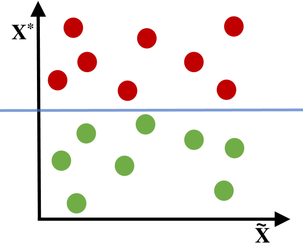
(a) real distribution

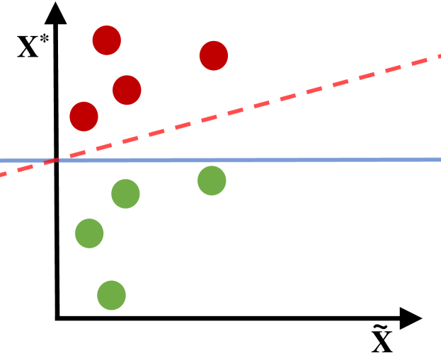
(b) marginal distribution shift

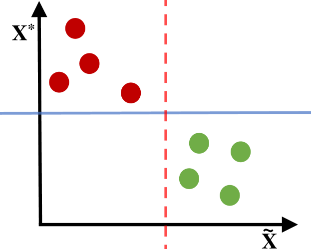
(c) conditional distribution shift

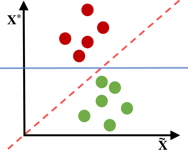
(d) joint distribution shift

Figure 1: Illustration of three types of distribution shift to generate OOD data. $X^{*}$ and $\widetilde{X}$ represent relevant and irrelevant features respectively. The colors of red and green dots represent two different classes. The blue solid line means the optimal decision rule and red dotted lines represent decision rules that model learn from the shifted data.

The last few years have witnessed human-level performance of deep network models under experimental test in various tasks like image recognition, speech processing and reading comprehension [16, 39]. However, in practical industrial implementations when the real-world data deviates from the observed training data, the model performance significantly declines and even sometimes completely fails [40, 45, 19, 22]. Extensive efforts have been taken to bridge the distribution gap between real-world data and training data to guarantee practical performance. Typical solutions include domain generalization [10, 11, 29, 32], causal learning [35, 36, 36], stable learning [42, 53], etc.

Other than developing methods to improve the experiment-practical generalization capability, few attention has been paid to the issue of model testing and address questions like “why the experimental testing results fail to reflect the real performance in practical implementation?” We argue that the practical implementation relies on models’ capability to handle Out-Of-Distribution (OOD) data, while experimental test essentially evaluates In-Distribution (ID) capability of models where training and test data follow the identical distribution. This study attempts to address the following three specific questions:

• What are the problems of ID test?

• Why ID test fails to reflect the practical implementation performance?

• How to evaluate the practical implementation performance under experimental test?

To facilitate these analyses, we first introduce a unified perspective to simulate the distribution shift between the observed training data and unseen test data. Specifically, three types of distribution shift are considered: (1) marginal distribution shift which refers to changes in the marginal distributions of irrelevant features between the training and test data; (2) conditional distribution shift which refers to changes in conditional distributions of labels when irrelevant features are given; and (3) joint distribution shift which suffers both the above situations. As illustrated in the toy example in Figure 1, these distribution shifts represent typical ways to construct OOD data and mislead the model to learn non-optimal parameters for OOD generalization. Following this categorization, we construct three ID settings and the corresponding OOD settings of training and test set on CelebA [30] and Colored MNIST [3]. The analysis into the result difference between ID settings and OOD settings address the above first question and observes the following problems of ID test: (1) ID test result cannot reflect models’ absolute OOD performance, (2) ID test result cannot compare between different models’ relative OOD performance.

Following the observations on the problems of ID test, we further ascribe the reason that ID test fails to reflect the practical implementation performance to the spurious correlations that model learned when training. Corresponding to the marginal and conditional distribution shifts, two types of spurious correlations are discussed: (1) marginal spurious correlation that irrelevant features are employed, and (2) conditional spurious correlation that incorrect feature-label correlations are employed. Experiment validates the performance decline on OOD data resulted from the different spurious correlations. Finally, we propose practical OOD test paradigms to evaluate generalization capability of models to unseen data using the observed data. We discuss test paradigms for both scenarios when irrelevant features are known and unknown using different OOD data settings. Moreover, the derived OOD test results gain access to identify what irrelevant features critically influence the model performance (i.e., finding bugs), and provide guideline to develop targeted solutions for performance improvement (i.e., debugging). It is desired to consider the test module beyond simply evaluation and form a closed loop between testing and debugging to promote the model performance in practical implementation.

The main contributions of this paper are as follows:

• We introduce a unified perspective to simulate OOD data construction into three types of distribution shift. Experimental analysis observes the problems of ID test under corresponding distribution shift settings.

• We explore the reasons of ID test failure as two types of learned spurious correlations. The discussions on spurious correlations illustrate their differences in effects on the generalization capability of models.

• We propose novel OOD test paradigms to evaluate the models’ performance in handling unseen data. This opens possibility to employ the proposed OOD test to help identify critical irrelevant features.

2 A Unified Perspective of Out-of-Distribution Data

In this section, we first introduce the concepts of IID-based supervised learning and out-of-distribution data. We then propose a novel and unifying view on categorization of distribution shift. Further, we construct three ID settings and the corresponding OOD settings of training and test sets on two simple image classification datasets for experiments in Section 3.

IID-based Supervised Learning. Let $\mathcal{X}$ denotes the feature space and $\mathcal{Y}$ the label space. A predictive function or model is defined as $f_{\theta}:\mathcal{X}\rightarrow\mathcal{Y}$, which takes features as input and predicted labels as output. A loss function is defined as $\ell:\mathcal{Y}\times\mathcal{Y}\rightarrow[0,+\infty)$. A data distribution is defined as $P(X,Y)$ which means a joint distribution on $\mathcal{X}\times\mathcal{Y}$. The context of supervised learning usually assumes that there exists a set of training samples $S=\{(x_{i},y_{i})\}_{i}^{N}$ with $(x_{i},y_{i})$ following $P_{tr}(X,Y)$. The goal is to find a set of optimal parameters $\Theta$ which minimize the risk $\mathbb{E}_{(x,y)\sim P_{te}}[\ell(f_{\Theta}(x),y)]$, where $P_{te}$ means test data distribution. Since we only have access to the training distribution $P_{tr}(X,Y)$ via the dataset $S$, the test distribution $P_{te}$ remains unseen to us. We instead search a predictor minimizing the empirical risk

$$\mathbb{E}=\frac{1}{N}\sum_{i}^{N}\ell(f_{\Theta}(x_{i}),y_{i}),$$ (1)

which assumes that the training samples and test samples are both independent and identically distributed (IID) [47].

Out-of-Distribution Data. Although the IID assumption allows us to train a model more conveniently, this assumption is difficult to be satisfied in reality. The distribution of test data can be distinct from the distribution of training data (i.e., out-of-distribution)[38], namely

$$P_{tr}(X,Y)\neq P_{te}(X,Y).$$ (2)

2.1 Three Types of Distribution Shift

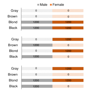
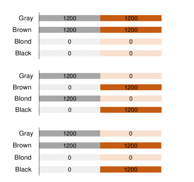
(a) CelebA

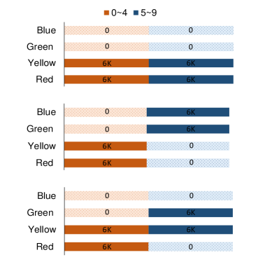
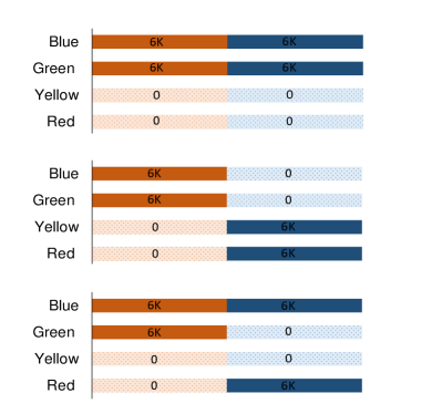
(b) Colored MNIST

Figure 2: Demonstration of three types of distribution shift on CelebA and Colored MNIST. From top to bottom, there are three pairs of training and test data with different settings which represent marginal, conditional, and joint distribution shifts.

Some works assume that the cause of the distribution shift is covariate shift [5], that is $P_{tr}(Y|X)=P_{te}(Y|X)$ and $P_{tr}(X)\neq P_{te}(X)$, of which we think as not comprehensive. In general, for most deep learning tasks, we categorize features into relevant features $X^{*}$ and irrelevant features $\widetilde{X}$. As shown in the Figure 1(a), the relevant features determine the real correspondence of input data and label. For example, determining which species a cat belongs to is relevant to its pattern and coat, not to its background, nor whether it is jumping or sleeping. We further make some reasonable assumptions to simplify Equation 2.

Assumption 1. Distribution of relevant features is invariant both in training and test data (e.g., all Ragdoll cats have blue eyes), which means $P(X^{*},Y)$ remains unchanged .

Assumption 2. Relevant features and irrelevant features are conditionally independent when label is given, denoted as $X^{*}\Vbar\widetilde{X}\mid Y$:

$$P(X^{*},\widetilde{X}|Y)=P(X^{*}|Y)P(\widetilde{X}|Y).$$ (3)

Assumption 3. There is no label shift [12] between training data and test data, denoted as $P_{tr}(Y)=P_{te}(Y)$.

With these assumptions, we can rewrite $P(X,Y)$ as

$$P(X^{*},\widetilde{X},Y) =\frac{P(X^{*},Y)P(\widetilde{X},Y)}{P(Y)},$$ (4)

and the essential distribution shift between training and test data is the shift of $P(\widetilde{X},Y)$ between them. According to the joint probability formula, we have:

$$P(\widetilde{X},Y)=P(\widetilde{X})P(Y|\widetilde{X}).$$ (5)

Therefore, there are three ways to construct OOD test set, that is, distribution shift between training and test data can be divided into three types:

• 1) Marginal distribution shift on $\widetilde{X}$. As shown in Figure 1(b), $P(\widetilde{X})$ changes while $P(Y|\widetilde{X})$ remains unchanged;

• 2) Conditional distribution shift on $Y$ when $\widetilde{X}$ is given. As shown in Figure 1(c), $P(Y|\widetilde{X})$ changes while $P(\widetilde{X})$ remains unchanged;

• 3) Joint distribution shift, a combination of 1) and 2). $P(Y|\widetilde{X})$ and $P(\widetilde{X})$ both change, as shown in Figure 1(d).

Taking a binary classification task of dogs and cats as an example, we consider backgrounds as irrelevant features. Suppose the backgrounds have four types: in cage, at home, on grass and on snow. If available data only cover one or two types of background, there occurs marginal distribution shift. If we get all four types of background, but the backgrounds are correlated with the labels (e.g., cats all in cages or at home, dogs all on grass or snow), a conditional distribution shift occurs. The joint distribution shift occurs when it suffers both the above situations. For example, the backgrounds of available data are not full-scale and partly correspond to labels. As depicted in Figure 1, in these cases, the model can learn red lines that deviate from optimum blue ones, which achieve high accuracy on in-distribution data but cannot generalize to out-of-distribution data.

2.2 OOD Dataset Setting

Table 1: In- and out-of-distribution accuracy of models and the decline ratio among them.

		Marginal distribution shift			Conditional distribution shift			Joint distribution shift
		ID	OOD	Drop%	ID	OOD	Drop%	ID	OOD	Drop%
CelebA	ResNet18 [16]	96.68	84.64	$\downarrow$12.45	99.36	25.27	$\downarrow$74.57	96.29	59.31	$\downarrow$38.40
	AlexNet [26]	98.33	88.91	$\downarrow$9.58	98.75	26.93	$\downarrow$72.73	97.08	69.79	$\downarrow$28.11
	Vgg11 [43]	99.02	91.32	$\downarrow$7.78	98.70	33.70	$\downarrow$65.86	97.40	71.36	$\downarrow$26.74
	DensNet121 [24]	97.27	89.31	$\downarrow$8.18	99.80	24.15	$\downarrow$75.80	97.66	71.38	$\downarrow$26.91
	SqueezeNet1.0 [25]	97.96	86.65	$\downarrow$11.55	98.74	22.48	$\downarrow$77.23	96.07	63.73	$\downarrow$33.66
	ResNeXt50 [51]	97.85	86.04	$\downarrow$12.07	99.41	37.52	$\downarrow$62.26	97.27	70.31	$\downarrow$27.72
	Average	97.85	87.81	$\downarrow$10.26	99.13	28.34	$\downarrow$71.41	96.96	67.65	$\downarrow$30.23
Colored Mnist	ResNet18 [16]	96.80	49.51	$\downarrow$48.85	98.17	0.21	$\downarrow$99.79	97.20	7.00	$\downarrow$92.80
	SqueezeNet1.0 [25]	97.87	37.07	$\downarrow$62.12	98.33	0.03	$\downarrow$99.97	97.90	32.28	$\downarrow$67.03
	SqueezeNet1.1 [25]	86.96	26.83	$\downarrow$69.15	97.77	0.00	$\downarrow$100.00	96.90	13.46	$\downarrow$86.11
	ResNet34 [16]	98.00	41.21	$\downarrow$57.95	98.77	0.40	$\downarrow$99.60	98.13	23.20	$\downarrow$76.36
	MobileNet v3 [23]	89.76	34.85	$\downarrow$61.17	95.17	0.78	$\downarrow$99.18	93.13	28.39	$\downarrow$69.52
	Average	93.88	37.90	$\downarrow$59.63	97.64	0.28	$\downarrow$99.71	96.65	20.87	$\downarrow$78.41

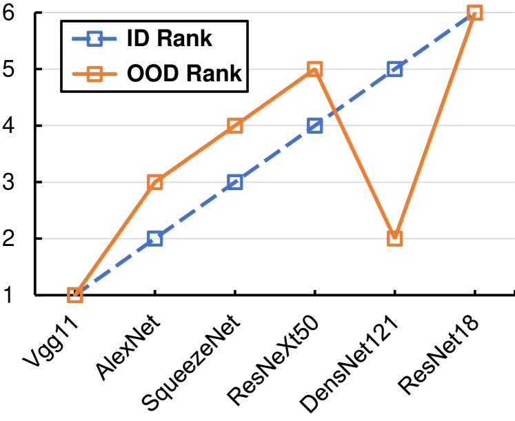
(a) Marginal distribution shift

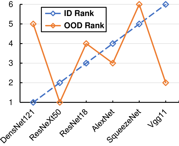
(b) Conditional distribution shift

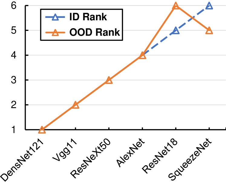
(c) Joint distribution shift

Figure 3: Illustration of the ID rank and OOD rank of several models under three distribution shifts on CelebA.

To investigate how models based on the IID assumption perform on OOD data, we choose two simple image classification datasets, CelebA [30] and Colored MNIST [3], on which we construct the above three types of distribution shift.

• CelebA [30] is a large-scale face dataset, each image with 40 attributes, and always used in Fairness area [37, 49]. In our experimental setting, we pick genders as labels and select 9,600 images in which the proportion of male and female is balanced. For either gender, there are four types of hair colors: black, blond, brown and gray, each being 1,200. Then we consider hair colors as irrelevant features and construct three pairs of dataset, each pair with a training set and an out-of-distribution test set. For instance, we select samples with blond and black hairs as training set, and make left samples test set to build marginal distribution shift. See detailed settings in Figure 2(a).

• Colored MNIST [3] is a colored MNIST handwritten digits dataset. In our experiment, we expand the digits colors of [3] to four types: red, yellow, green, and blue. The number of each digits category is the same as the original MNIST [27], and each color accounts for a quarter in each digit category, roughly 7,500 samples per color. Similar to the setting of CelebA, we construct three pairs of datasets to correspond to three distribution shifts. See detailed settings in Figure 2(b).

3 The Problem of ID Test

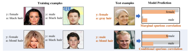
Figure 4: Examples of the two spurious correlations: (top) marginal spurious correlation; and (bottom) conditional spurious correlation. In the legend, gray and orange bars indicate probability of models’ predictions for in- and out-of-distribution samples respectively.

One of the main goals of training deep network models is to make the models generalize in the wild. As obtaining in-the-wild test data is expensive and time-consuming, most works use ID test data, that is, randomly splitting a portion of the training data as test data, to evaluate the models. In this section, we evaluate the performance of several ID test-based models under different distribution shifts and find several shortcomings of the ID test. See results in Table 1 and Figure 3.

Accuracy of ID Test is Not Accurate. Similar to results of [40, 18, 20], models with high accuracy on in-distribution data can fail on new distribution. From the results in Table 1, there shows a significant drop of accuracy in models when testing on OOD data. The accuracy drops range from 7.78% to 77.23% on CelebA and 48.85% to 100% on Colored MNIST. This demonstrates that the performance of the ID test cannot represent the real performance of the model, while the OOD test can reflect it to some extent. Furthermore, the models decline differently on the OOD test sets with different distribution shifts. Taking CelebA as a detailed example, the average drops of models accuracy under marginal distribution shift is 10.26%, while under conditional and joint distribution shifts, the number is 71.41% and 30.23% respectively, both higher than the first. This illustrates that different distribution shifts impair models’ performance in different degrees, so we need different types of OOD data for testing comprehensively. In short, the accuracy of ID test is not accurate, and we need OOD test to address this problem.

Rank of ID Test is Not Robust. Although ID accuracy cannot represent the real accuracy of the models, we hope that the rank of ID accuracy of models can help us pick the best one. However, in our experiment, we find that the ID rank of the models is not robust, i.e., cannot represent the OOD rank. For instance, Figure 3(b) shows that under conditional distribution shift the Vgg11 model has the lowest ID rank, but a relatively high OOD rank (only lower than ResNeXt50). Some prior works show that a model with high accuracy on in-distribution data will also achieve relatively high accuracy on out-of-distribution data [40, 31] which is inconsistent with our finding. We think they come to this result because the distribution shift between the OOD test data and training data they used is very small. Under our dataset partition settings, the marginal and conditional distribution shifts we construct are extreme, while the joint distribution shift is less extreme. Figure 3 shows that the ID ranks and OOD ranks of the models barely coincide under the marginal and conditional distribution shifts, while under the joint distribution shift the ranks almost coincide. In summary, ID test results cannot compare between different models’ relative OOD ranks, and the ranks are not consistent across different types of distribution shift, so we cannot only use a single OOD test set to evaluate the real performance of models.

4 Reasons that ID Test Fails

To better guide us to generate practical OOD test set, we need to know what causes the failure of ID test. We conclude that ID test fails as a result of two different spurious correlations, which are 1) marginal spurious correlation and 2) conditional spurious correlation. These two spurious correlations incur performance drop of models under marginal and conditional distribution shifts, respectively.

Definition 1. Given a dataset $\mathcal{D}$ with an irrelevant feature $\widetilde{x}\in\widetilde{X}$ which makes the conditional probability of any two labels $y_{i}$, $y_{j}$ equal, namely $p(y_{i}|\widetilde{x})=p(y_{j}|\widetilde{x})$. If a model trained on $\mathcal{D}$ use $\widetilde{x}$ as a discriminative feature when making decisions, we call the model has learned a marginal spurious correlation.

Definition 2. Given a dataset $\mathcal{D}$ with an irrelevant feature $\widetilde{x}\in\widetilde{X}$, there exists two $y_{i}$, $y_{j}$ whose conditional probability are not equal, namely $p(y_{i}|\widetilde{x})\neq p(y_{j}|\widetilde{x})$. If a model trained on $\mathcal{D}$ use $\widetilde{x}$ as a discriminative feature when making decisions, we call the model have learned a conditional spurious correlation.

Figure 4 shows an example, where $y$ represents the label of the image and $a$ represents the specific attribute of the irrelevant feature hair color. The top half of the Figure 4 shows that the model trained on the dataset with all black hairs has a drop in predictions probability when testing in dataset with all gray hairs (i.e., marginal spurious correlation); at the bottom half, the gender and hair color in test data has the opposite correspondence with the training set, and the model’s prediction result is also the opposite (i.e., conditional spurious correlation).

4.1 Marginal Spurious Correlation

Table 2: Results of ResNet18 and 2-layer CNN models on Colored MNIST in different contexts. R-1K represents the dataset which size is 1,000 with red color, similar settings to other datasets in the table. The bold part represents in-distribution accuracy.

	dataset	test-R	test-Y	test-G	test-B	Drop%
ResNet18	R-1K	98.90	27.10	11.60	9.10	$\downarrow$62.92
	Y-1K	34.80	98.80	42.70	28.70	$\downarrow$48.13
	G-1K	14.40	19.90	99.10	14.00	$\downarrow$62.82
	B-1K	23.10	12.40	18.40	99.10	$\downarrow$61.40
	R-Full	99.95	59.70	72.81	85.75	$\downarrow$20.40
	Y-Full	45.72	99.91	76.34	30.81	$\downarrow$36.75
	G-Full	57.75	83.19	99.92	68.43	$\downarrow$22.61
	B-Full	22.19	34.52	87.54	99.89	$\downarrow$38.90
2-layer CNN	R-1K	91.90	89.60	47.10	35.20	$\downarrow$28.24
	Y-1K	75.10	91.60	88.60	27.30	$\downarrow$22.87
	G-1K	80.20	90.70	92.80	62.00	$\downarrow$12.26
	B-1K	90.40	86.50	67.30	97.60	$\downarrow$12.26
	R-Full	99.90	93.16	42.86	82.95	$\downarrow$20.20
	Y-Full	98.62	99.91	98.15	53.33	$\downarrow$12.42
	G-Full	14.19	88.74	99.90	29.90	$\downarrow$41.76
	B-Full	99.23	89.52	29.00	99.87	$\downarrow$20.49

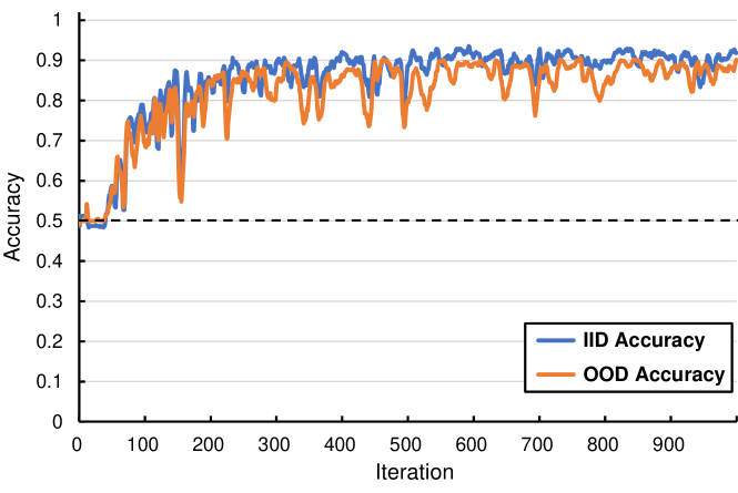
(a) Marginal Spurious Correlation

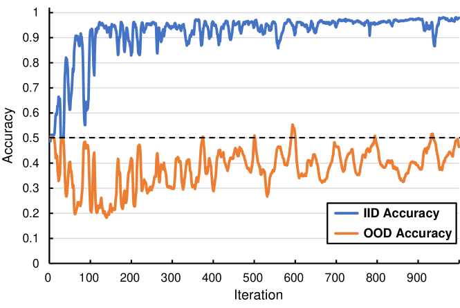
(b) Conditional Spurious Correlation

Figure 5: Comparison of the model accuracy between on the in-distribution validation set and on the out-of-distribution test set.

From the results in Table 1, it can be seen that the accuracy of models declines on the OOD test set with marginal distribution shift, which is not in line with human intuition. Intuitively, the models should not use an irrelevant feature as a discriminative feature when the irrelevant feature and label are not correlated in the training data. In other words the model performance should not be affected even if the distribution of the irrelevant feature shifts in the test set. We suspect the reason for the experimental phenomenon contradicting intuition is that the deep models have learned the marginal spurious correlation.

To verify this point, we construct two groups of data based on MNIST [27]. The first group randomly selects 1,000 images from MNIST and creates 4 copies of different colors: red, yellow, green and blue. So these four copies are consistent except for digits colors. The second group uses the full MNIST samples, and the color settings are the same as the first group. We train a ResNet18 model and a 2-layer CNN model on the above two groups of data, using one copy for training each time, and the other copies for testing. We report ID validation accuracy, OOD test accuracy and the average drop rate of the two models in Table 2.

The results in Table 2 show that: 1) whether the model size is large or small, performance drops when training on one color and testing on other colors, indicating that the models have learned marginal spurious correlations; 2) as [18, 45] find that diverse training data can improve models’ robustness to image corruptions and dataset shift, we find the increase of training data reduce the models’ learning of marginal spurious correlations. For example, the accuracy of the ResNet18 trained on R-Full drops by an average of 20.4% in other color settings, which is 1/3 of that trained on R-1K; 3) while [18] suggests that larger models can reduce the gap between ID accuracy and OOD accuracy, we find that larger models are more likely to learn marginal spurious correlation than small models. For example, the average drop rate of the 2-layer CNN model on OOD test sets is much smaller than that of ResNet18.

To explain why the model exhibits such counter-intuitive behavior, part of the clues already exist in [44, 33]: the gradient descent-based optimization algorithm used for model training can have a slow logarithmic rate of convergence, and it usually cannot find the optimal parameters. Even if an irrelevant feature does not correlate with the label in the data, the model trained by gradient descent can unintentionally use it as a discriminative feature. See illustration in Figure 1(b).

4.2 Conditional Spurious Correlation

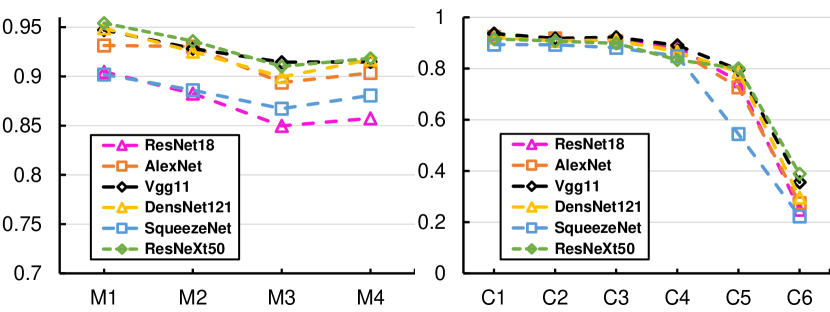
(a) CelebA

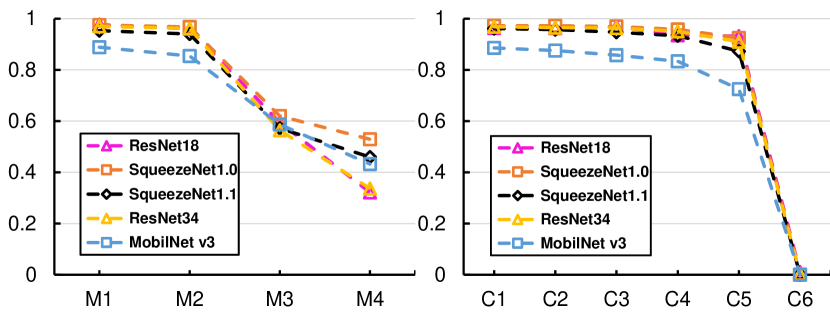
(b) Colored MNIST

Figure 6: Performance of models under different levels of distribution shift. We construct 4 levels of marginal distribution shift, $M1$ ~$M4$, by varying the proportion of hair colors (or digits colors) in the datasets; and six levels of conditional distribution shift, $C1$ ~$C6$, by changing the correlation degrees between hair colors (or digits colors) and labels.

The models are greatly affected by the conditional distribution shift. For example, ResNet18 can achieve the accuracy of 99.36% on ID validation set of CelebA but only the accuracy of 27% on the OOD test set. We consider that the model intentionally learns the conditional spurious correlation employing incorrect feature-label correlations in the training set, and relies heavily on it when testing. To further explore how conditional spurious correlation affects model performance and how it differs from marginal spurious correlation, we report the accuracy for the first 1,000 iterations of ResNet18 with a batch size of 16 in two OOD settings (marginal and conditional distribution shifts). As shown in Figure 5(b), the model shows a polarization trend at the very beginning, and achieves ID accuracy of 95% and OOD accuracy of 20% in the early iterations. This demonstrates that in such an OOD setting, the model learns almost only conditional spurious correlations in early training. In contrast, Figure 5(a) shows there is a small gap between ID accuracy and OOD accuracy in the later iterations of training which indicates the model has a slower learning rate for marginal spurious correlation. Further, in Figure 5(b), after about 200 iterations, the ID accuracy of the model stabilizes and there is a small rebound in OOD accuracy which always stays below 50%. This indicates that as the training progresses, the model can slightly reduces the use of conditional spurious correlations.

5 Towards OOD Test

While a lot of works are devoted to improving the OOD generalization of models, there is still a great gap in how to evaluate the model performance in handling unseen OOD data. In this section, we propose OOD test paradigms for both scenarios when irrelevant features are known and unknown, using different OOD data settings, and we discuss how to use OOD test results to find bugs in models and guide debugging.

5.1 Evaluation with Different Levels and Types of OOD Test Set

Since the models can be affected by spurious correlations during training (see Section 4), we cannot use ID performance to measure the real OOD performance of the model. Although some prior works have already recognized the importance of OOD test [1, 2, 4, 15, 46], their test methods are incomplete, such as using only one single OOD test set for evaluation. As distribution shifts in practical scenarios are diverse, we suggest constructing OOD test sets with different levels and types of distribution shift to more comprehensively and accurately evaluate the OOD performance of the models.

To prove the effectiveness, we construct two types and multiple levels distribution shifts on CelebA and Colored MNIST to evaluate the OOD performance of several models. As shown in Figure 6, as the degree of distribution shifts increases, the performance of the models is basically declining. Specifically, as the degree of marginal distribution shifts increases, the model performance decreases at a nearly linear trend, indicating that the model is progressively more influenced by the marginal spurious correlation. However, as the degree of conditional distribution shifts increases, the model is less affected at the beginning and has a sharp drop at the late stage indicates that the model is strongly influenced by conditional spurious correlations in extreme settings. With these results, we can infer the possible performance of these models in practical scenarios, helping us to anticipate the possible risks.

5.2 Evaluation with Clustered OOD Test Set

Table 3: Comparison of accuracy of ResNet18 and SqueezeNet on clustered Colored MNIST.

	ID Acc		OOD Acc (Avg)
	ResNet18	SqueezeNet	ResNet18	SqueezeNet
D1	96.06	96.62	94.37	95.59
D2	94.56	96.30	87.22	93.91
D3	97.75	96.77	43.19	43.17
D4	96.59	96.42	37.79	42.40
D5	95.39	95.39	41.65	50.99
D6	94.67	94.67	56.17	59.14
D7	91.84	94.56	43.60	61.75
D8	79.07	86.05	34.86	43.14

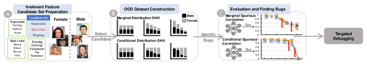
Figure 7: Employing OOD test to find bugs for deep network models.

Knowing the labels and specific irrelevant features of the data (e.g., NICO [17] gives both labels and backgrounds of the images), we can directly use the features to construct different types and levels of OOD test sets. But in general, we have only the raw data without irrelevant features that can be used directly. In such a scenario, we suggest clustering the data to construct OOD test sets with implicit distribution shifts.

We use a ResNet50 pre-trained at ImageNet as the feature extractor, and the input vectors of the fully-connected layer as the embedding representation of samples. We then cluster the samples of each category of Colored MNIST into 8 clusters in the embedding space, and combine them in order of cluster size to obtain 8 sub-datasets $(D_{i})_{i}^{N=8}$. We use one for training and the others for testing, and report ID accuracy and average OOD test accuracy in Table 3. The results show that different clustered OOD test sets bring different degrees of performance decline which demonstrates that clustered OOD data can evaluate the OOD performance of the models to some extent. And we can use these results to compare models to choose the better one. For example, a small model seems a better choice than a large model for the problem of colored handwritten digit recognition.

5.3 Discussions on Finding Bugs for Deep Network Models

Similar to software engineering, finding “bugs” in machine learning, i.e., which irrelevant features significantly undermine the performance, plays a critical role in testing before the model is deployed to production [6]. In current machine learning test, however, finding bugs is largely ignored. One reason is that, machine learning models, especially deep network models conduct end-to-end inference as a black-box fashion, making traditional testing paradigm such as unit testing in software engineering failed to be directly applied. In this section, we discuss the possibility of employing the proposed OOD test paradigm to identify the significantly harmful irrelevant features. The following elaborates the three steps of finding bugs for deep network models. This is illustrated in Figure 7.

Irrelevant Feature Candidate Set Preparation. The workflow starts with preparing a candidate set of all possible irrelevant features $(\widetilde{x}_{i})_{i}^{n}\subseteq\widetilde{X}$ for the examined task. For example, for the task of image gender classification, we may construct the candidate set consisting of irrelevant features concerning experssion, hair color, wearing, etc.

OOD Dataset Construction. Given one irrelevant feature to be tested, e.g., $\widetilde{x}_{i}=\mbox{hair color}$, we then construct OOD datasets by modifying the distribution of $\widetilde{x}_{i}$ with different types and levels .

Evaluation and Finding Bugs. Evaluation can be conducted on the above constructed different settings of OOD datasets. By examining the performance decline in different types/levels of distribution shifts, we can identify bugs in two levels: (1) whether the tested irrelevant feature is bug (i.e., siginicantly undermines the performance), (2) which type of spurious correlation the model learned and mainly relied on.

The above workflow iterates till we test all the candidate irrelevant features to derive the identified bugs for current deep network model. This enables targeted debugging and developing corresponding solutions for more effective model improvement. For example, the identified specific irrelevant feature (e.g., hair color) leads to data augmentation on balancing the distribution or model regularization on penalizing features regarding hair color.

6 Related Work

As models can significantly fail when the test distribution is distinct from the training distribution [40, 45, 19, 22], a range of advanced algorithms are proposed for OOD generalization, such as invariant representation learning [50, 7, 13, 10], feature disentanglement [28, 52, 34], adversarial data augmentation [41, 48, 54]. While these algorithms improve the OOD generalization of models under their own experimental settings, a recent work [14] finds that these algorithms may be overestimated, i.e., most advanced OOD generalization algorithms are only comparable with Empirical Risk Minimization (ERM) [47] when under the same experimental settings. Therefore, in addition to developing algorithms that improve the OOD generalization, it is also important to develop methods that can better evaluate the capability of algorithms to handle unseen OOD data.

A number of benchmarks have been introduced to develop OOD generalization in both CV [19, 17, 28, 8] and NLP [21, 31], but most of these benchmarks build only one type of distribution shift. DomainBed proposed by [14] includes several OOD generalization datasets, so it has a richer type of distribution shift, but not multi-level distribution shifts. This suggests that we need a new testing paradigm to test the OOD generalization capability of the models.

7 Conclusion

We propose practical OOD test paradigms to evaluate the OOD performance of the model and a workflow for finding bugs that can bring guidelines for model debugging. To accomplish this, we first introduce a unified categorization perspective of distribution shift between the observed training data and unseen test data, and find the problem of ID test: the ID performance cannot represent the OOD performance. We then ascribe the reason for IID test failures to marginal and conditional spurious correlation. We expect the test paradigms and workflow can lead to more focusing on the testing of models’ capabilities to handle OOD data.

References

- [1] Aishwarya Agrawal, Dhruv Batra, Devi Parikh, and Aniruddha Kembhavi. Don’t just assume; look and answer: Overcoming priors for visual question answering. In Proceedings of the IEEE Conference on Computer Vision and Pattern Recognition, pages 4971–4980, 2018.
- [2] Arjun R. Akula, Spandana Gella, Yaser Al-Onaizan, Song-Chun Zhu, and Siva Reddy. Words aren’t enough, their order matters: On the robustness of grounding visual referring expressions. In Proceedings of the 58th Annual Meeting of the Association for Computational Linguistics, ACL 2020, Online, July 5-10, 2020, pages 6555–6565. Association for Computational Linguistics, 2020.
- [3] Martin Arjovsky, Léon Bottou, Ishaan Gulrajani, and David Lopez-Paz. Invariant risk minimization. arXiv preprint arXiv:1907.02893, 2019.
- [4] Andrei Barbu, David Mayo, Julian Alverio, William Luo, Christopher Wang, Dan Gutfreund, Josh Tenenbaum, and Boris Katz. Objectnet: A large-scale bias-controlled dataset for pushing the limits of object recognition models. In Hanna M. Wallach, Hugo Larochelle, Alina Beygelzimer, Florence d’Alché-Buc, Emily B. Fox, and Roman Garnett, editors, Advances in Neural Information Processing Systems 32: Annual Conference on Neural Information Processing Systems 2019, NeurIPS 2019, December 8-14, 2019, Vancouver, BC, Canada, pages 9448–9458, 2019.
- [5] Shai Ben-David, John Blitzer, Koby Crammer, Alex Kulesza, Fernando Pereira, and Jennifer Wortman Vaughan. A theory of learning from different domains. Machine learning, 79(1):151–175, 2010.
- [6] David Berend, Xiaofei Xie, Lei Ma, Lingjun Zhou, Yang Liu, Chi Xu, and Jianjun Zhao. Cats are not fish: Deep learning testing calls for out-of-distribution awareness. In Proceedings of the 35th IEEE/ACM International Conference on Automated Software Engineering, pages 1041–1052, 2020.
- [7] Gilles Blanchard, Gyemin Lee, and Clayton Scott. Generalizing from several related classification tasks to a new unlabeled sample. Advances in neural information processing systems, 24:2178–2186, 2011.
- [8] Chen Fang, Ye Xu, and Daniel N Rockmore. Unbiased metric learning: On the utilization of multiple datasets and web images for softening bias. In Proceedings of the IEEE International Conference on Computer Vision, pages 1657–1664, 2013.
- [9] João Gama, Indrė Žliobaitė, Albert Bifet, Mykola Pechenizkiy, and Abdelhamid Bouchachia. A survey on concept drift adaptation. ACM computing surveys (CSUR), 46(4):1–37, 2014.
- [10] Yaroslav Ganin and Victor Lempitsky. Unsupervised domain adaptation by backpropagation. In International conference on machine learning, pages 1180–1189. PMLR, 2015.
- [11] Yaroslav Ganin, Evgeniya Ustinova, Hana Ajakan, Pascal Germain, Hugo Larochelle, François Laviolette, Mario Marchand, and Victor Lempitsky. Domain-adversarial training of neural networks. The journal of machine learning research, 17(1):2096–2030, 2016.
- [12] Saurabh Garg, Yifan Wu, Sivaraman Balakrishnan, and Zachary C. Lipton. A unified view of label shift estimation. In Hugo Larochelle, Marc’Aurelio Ranzato, Raia Hadsell, Maria-Florina Balcan, and Hsuan-Tien Lin, editors, Advances in Neural Information Processing Systems 33: Annual Conference on Neural Information Processing Systems 2020, NeurIPS 2020, December 6-12, 2020, virtual, 2020.
- [13] Muhammad Ghifary, W Bastiaan Kleijn, Mengjie Zhang, and David Balduzzi. Domain generalization for object recognition with multi-task autoencoders. In Proceedings of the IEEE international conference on computer vision, pages 2551–2559, 2015.
- [14] Ishaan Gulrajani and David Lopez-Paz. In search of lost domain generalization. In International Conference on Learning Representations, 2020.
- [15] Yangyang Guo, Zhiyong Cheng, Liqiang Nie, Yibing Liu, Yinglong Wang, and Mohan Kankanhalli. Quantifying and alleviating the language prior problem in visual question answering. In Proceedings of the 42nd International ACM SIGIR Conference on Research and Development in Information Retrieval, pages 75–84, 2019.
- [16] Kaiming He, Xiangyu Zhang, Shaoqing Ren, and Jian Sun. Deep residual learning for image recognition. In Proceedings of the IEEE conference on computer vision and pattern recognition, pages 770–778, 2016.
- [17] Yue He, Zheyan Shen, and Peng Cui. Towards non-iid image classification: A dataset and baselines. Pattern Recognition, 110:107383, 2021.
- [18] Dan Hendrycks, Steven Basart, Norman Mu, Saurav Kadavath, Frank Wang, Evan Dorundo, Rahul Desai, Tyler Zhu, Samyak Parajuli, Mike Guo, Dawn Song, Jacob Steinhardt, and Justin Gilmer. The many faces of robustness: A critical analysis of out-of-distribution generalization. ICCV, 2021.
- [19] Dan Hendrycks and Thomas Dietterich. Benchmarking neural network robustness to common corruptions and perturbations. arXiv preprint arXiv:1903.12261, 2019.
- [20] Dan Hendrycks, Xiaoyuan Liu, Eric Wallace, Adam Dziedzic, Rishabh Krishnan, and Dawn Song. Pretrained transformers improve out-of-distribution robustness. In Proceedings of the 58th Annual Meeting of the Association for Computational Linguistics, pages 2744–2751, Online, July 2020. Association for Computational Linguistics.
- [21] Dan Hendrycks, Xiaoyuan Liu, Eric Wallace, Adam Dziedzic, Rishabh Krishnan, and Dawn Song. Pretrained transformers improve out-of-distribution robustness. In Proceedings of the 58th Annual Meeting of the Association for Computational Linguistics, pages 2744–2751, 2020.
- [22] Dan Hendrycks, Kevin Zhao, Steven Basart, Jacob Steinhardt, and Dawn Song. Natural adversarial examples. In Proceedings of the IEEE/CVF Conference on Computer Vision and Pattern Recognition, pages 15262–15271, 2021.
- [23] Andrew G Howard, Menglong Zhu, Bo Chen, Dmitry Kalenichenko, Weijun Wang, Tobias Weyand, Marco Andreetto, and Hartwig Adam. Mobilenets: Efficient convolutional neural networks for mobile vision applications. arXiv preprint arXiv:1704.04861, 2017.
- [24] Gao Huang, Zhuang Liu, Laurens Van Der Maaten, and Kilian Q Weinberger. Densely connected convolutional networks. In Proceedings of the IEEE conference on computer vision and pattern recognition, pages 4700–4708, 2017.
- [25] Forrest N Iandola, Song Han, Matthew W Moskewicz, Khalid Ashraf, William J Dally, and Kurt Keutzer. Squeezenet: Alexnet-level accuracy with 50x fewer parameters and¡ 0.5 mb model size. arXiv preprint arXiv:1602.07360, 2016.
- [26] Alex Krizhevsky, Ilya Sutskever, and Geoffrey E Hinton. Imagenet classification with deep convolutional neural networks. Advances in neural information processing systems, 25:1097–1105, 2012.
- [27] Yann LeCun, Léon Bottou, Yoshua Bengio, and Patrick Haffner. Gradient-based learning applied to document recognition. Proceedings of the IEEE, 86(11):2278–2324, 1998.
- [28] Da Li, Yongxin Yang, Yi-Zhe Song, and Timothy M Hospedales. Deeper, broader and artier domain generalization. In Proceedings of the IEEE international conference on computer vision, pages 5542–5550, 2017.
- [29] Haoliang Li, Sinno Jialin Pan, Shiqi Wang, and Alex C Kot. Domain generalization with adversarial feature learning. In Proceedings of the IEEE Conference on Computer Vision and Pattern Recognition, pages 5400–5409, 2018.
- [30] Ziwei Liu, Ping Luo, Xiaogang Wang, and Xiaoou Tang. Deep learning face attributes in the wild. In Proceedings of the IEEE international conference on computer vision, pages 3730–3738, 2015.
- [31] John Miller, Karl Krauth, Benjamin Recht, and Ludwig Schmidt. The effect of natural distribution shift on question answering models. In International Conference on Machine Learning, pages 6905–6916. PMLR, 2020.
- [32] Saeid Motiian, Marco Piccirilli, Donald A Adjeroh, and Gianfranco Doretto. Unified deep supervised domain adaptation and generalization. In Proceedings of the IEEE international conference on computer vision, pages 5715–5725, 2017.
- [33] Vaishnavh Nagarajan, Anders Andreassen, and Behnam Neyshabur. Understanding the failure modes of out-of-distribution generalization. In 9th International Conference on Learning Representations, ICLR 2021, Virtual Event, Austria, May 3-7, 2021. OpenReview.net, 2021.
- [34] Li Niu, Wen Li, and Dong Xu. Multi-view domain generalization for visual recognition. In Proceedings of the IEEE international conference on computer vision, pages 4193–4201, 2015.
- [35] Jonas Peters, Peter Bühlmann, and Nicolai Meinshausen. Causal inference by using invariant prediction: identification and confidence intervals. Journal of the Royal Statistical Society. Series B (Statistical Methodology), pages 947–1012, 2016.
- [36] Niklas Pfister, Peter Bühlmann, and Jonas Peters. Invariant causal prediction for sequential data. Journal of the American Statistical Association, 114(527):1264–1276, 2019.
- [37] Novi Quadrianto, Viktoriia Sharmanska, and Oliver Thomas. Discovering fair representations in the data domain. In Proceedings of the IEEE/CVF Conference on Computer Vision and Pattern Recognition, pages 8227–8236, 2019.
- [38] Joaquin Quiñonero-Candela, Masashi Sugiyama, Neil D Lawrence, and Anton Schwaighofer. Dataset shift in machine learning. Mit Press, 2009.
- [39] Pranav Rajpurkar, Robin Jia, and Percy Liang. Know what you don’t know: Unanswerable questions for squad. In Iryna Gurevych and Yusuke Miyao, editors, Proceedings of the 56th Annual Meeting of the Association for Computational Linguistics, ACL 2018, Melbourne, Australia, July 15-20, 2018, Volume 2: Short Papers, pages 784–789. Association for Computational Linguistics, 2018.
- [40] Benjamin Recht, Rebecca Roelofs, Ludwig Schmidt, and Vaishaal Shankar. Do imagenet classifiers generalize to imagenet? In International Conference on Machine Learning, pages 5389–5400. PMLR, 2019.
- [41] Shiv Shankar, Vihari Piratla, Soumen Chakrabarti, Siddhartha Chaudhuri, Preethi Jyothi, and Sunita Sarawagi. Generalizing across domains via cross-gradient training. In International Conference on Learning Representations, 2018.
- [42] Zheyan Shen, Peng Cui, Tong Zhang, and Kun Kunag. Stable learning via sample reweighting. In Proceedings of the AAAI Conference on Artificial Intelligence, volume 34, pages 5692–5699, 2020.
- [43] Karen Simonyan and Andrew Zisserman. Very deep convolutional networks for large-scale image recognition. In Yoshua Bengio and Yann LeCun, editors, 3rd International Conference on Learning Representations, ICLR 2015, San Diego, CA, USA, May 7-9, 2015, Conference Track Proceedings, 2015.
- [44] Daniel Soudry, Elad Hoffer, Mor Shpigel Nacson, Suriya Gunasekar, and Nathan Srebro. The implicit bias of gradient descent on separable data. The Journal of Machine Learning Research, 19(1):2822–2878, 2018.
- [45] Rohan Taori, Achal Dave, Vaishaal Shankar, Nicholas Carlini, Benjamin Recht, and Ludwig Schmidt. Measuring robustness to natural distribution shifts in image classification. In Hugo Larochelle, Marc’Aurelio Ranzato, Raia Hadsell, Maria-Florina Balcan, and Hsuan-Tien Lin, editors, Advances in Neural Information Processing Systems 33: Annual Conference on Neural Information Processing Systems 2020, NeurIPS 2020, December 6-12, 2020, virtual, 2020.
- [46] Damien Teney, Ehsan Abbasnejad, Kushal Kafle, Robik Shrestha, Christopher Kanan, and Anton van den Hengel. On the value of out-of-distribution testing: An example of goodhart’s law. In Hugo Larochelle, Marc’Aurelio Ranzato, Raia Hadsell, Maria-Florina Balcan, and Hsuan-Tien Lin, editors, Advances in Neural Information Processing Systems 33: Annual Conference on Neural Information Processing Systems 2020, NeurIPS 2020, December 6-12, 2020, virtual, 2020.
- [47] Vladimir Vapnik and Vlamimir Vapnik. Statistical learning theory wiley. New York, 1(624):2, 1998.
- [48] Riccardo Volpi, Hongseok Namkoong, Ozan Sener, John C Duchi, Vittorio Murino, and Silvio Savarese. Generalizing to unseen domains via adversarial data augmentation. In NeurIPS, 2018.
- [49] Zeyu Wang, Klint Qinami, Ioannis Christos Karakozis, Kyle Genova, Prem Nair, Kenji Hata, and Olga Russakovsky. Towards fairness in visual recognition: Effective strategies for bias mitigation. In Proceedings of the IEEE/CVF conference on computer vision and pattern recognition, pages 8919–8928, 2020.
- [50] Zhen Wang, Qiansheng Wang, Chengguo Lv, Xue Cao, and Guohong Fu. Unseen target stance detection with adversarial domain generalization. In 2020 International Joint Conference on Neural Networks (IJCNN), pages 1–8. IEEE, 2020.
- [51] Saining Xie, Ross Girshick, Piotr Dollár, Zhuowen Tu, and Kaiming He. Aggregated residual transformations for deep neural networks. In Proceedings of the IEEE conference on computer vision and pattern recognition, pages 1492–1500, 2017.
- [52] Zheng Xu, Wen Li, Li Niu, and Dong Xu. Exploiting low-rank structure from latent domains for domain generalization. In European Conference on Computer Vision, pages 628–643. Springer, 2014.
- [53] Xingxuan Zhang, Peng Cui, Renzhe Xu, Linjun Zhou, Yue He, and Zheyan Shen. Deep stable learning for out-of-distribution generalization. In Proceedings of the IEEE/CVF Conference on Computer Vision and Pattern Recognition, pages 5372–5382, 2021.
- [54] Kaiyang Zhou, Yongxin Yang, Timothy Hospedales, and Tao Xiang. Deep domain-adversarial image generation for domain generalisation. In Proceedings of the AAAI Conference on Artificial Intelligence, volume 34, pages 13025–13032, 2020.