Populating the landscape in an inhomogeneous Universe

Abstract

The primordial Universe might be highly inhomogeneous. We perform the 3+1D Numerical Relativity simulation for the evolution of scalar field in an initial inhomogeneous expanding Universe, and investigate how it populates the landscape with both de Sitter (dS) and AdS vacua. The simulation results show that eventually either the field in different region separates into different vacua, so that the expanding dS or AdS bubbles (the bubble wall is expanding but the spacetime inside AdS bubbles is contracting) come into being with clear bounderies, or overall region is dS expanding with a few smaller AdS bubbles (which collapsed into black holes) or inhomogeneously collapsing.

I Introduction

It has been widely thought that the inflation Guth (1981); Linde (1982); Albrecht and Steinhardt (1982); Starobinsky (1980); Sato (1981); Fang (1980), which may be well approximated by a de Sitter (dS) spacetime, should happen at the early epoch of our Universe. The current accelerated expansion of our Universe also suggests that it has a dS-like dark energy referred as the cosmological constant. However, a stable dS state seems not favorable in the String landscape Bousso and Polchinski (2000); Susskind (2003), which if exists, might be extremely rare, see Ooguri and Vafa (2007); Obied et al. (2018) for the swampland conjecture. In contrast, it is easy to construct Anti-dS (AdS) vacua, Bousso and Polchinski (2000); Danielsson et al. (2009), see e.g.Piao (2004); Piao and Zhang (2005); Garriga et al. (2013); Blanco-Pillado et al. (2020); Li et al. (2020); Ye and Piao (2020a, b) for the implications of AdS vacua on early Universe.

In such a landscape (AdS and dS vacua coexist), see Fig.1, whether it is possible for our Universe to evolve to the corresponding dS vacua and whether it is possible for it to stay in a dS state consistent with the current observations is not obvious. Thus how to populate the landscape, especially how our Universe started from a dS-like inflation when AdS vacua exist, has still been a concerned issue. It has been showed in Refs.Coleman (1977); Coleman and De Luccia (1980) that in an effective potential with multiple vacua, the nucleation of bubbles with different vacua can spontaneously occur, see also e.g.Blau et al. (1987); Lee and Weinberg (1987); Linde (1992); Easther et al. (2009); Brown and Dahlen (2011); Braden et al. (2019). Recent Refs.Blanco-Pillado et al. (2019); Huang and Ford (2020); Wang (2019) have also reported the possibility that a large velocity fluctuation of the scalar field pushes a region of field over the potential barrier.

However, it is usually speculated that the primordial Universe is highly inhomogeneous, i.e. the scalar field or spacetime metric has large inhomogeneities before a region of space arrived at certain vacuum. The large inhomogeneities might also be present in multi-stream inflation Li and Wang (2009); Li et al. (2009), in which the inflaton field rolled along a multiple-branch path, so that the homogeneities might hardly be preserved after bifurcations, see also recent Cai et al. (2021). Recently, in the studies concerning large inhomogeneities, Numercial Relativity (NR), see Lehner and Pretorius (2014); Cardoso et al. (2015); Palenzuela (2020) for recent reviews, has become a powerful and indispensable tool Giblin et al. (2016); Macpherson et al. (2017, 2019); Giblin and Tishue (2019); Kou et al. (2021), see also its application to the beginning of inflation East et al. (2016); Clough et al. (2017, 2018); Aurrekoetxea et al. (2020); Joana and Clesse (2021), cosmological bubble collisions Johnson et al. (2012); Wainwright et al. (2014a, b); Johnson et al. (2016), cosmological solitonsNazari et al. (2021) and primordial black holes de Jong et al. (2021).

It is interesting and significant to perform the 3+1D NR simulation in an initial inhomogeneous Universe to investigate how the scalar field populates the landscape. We will work with a highly inhomogeneous Universe that is initially expanding and a scalar field (its effective potential has both dS and AdS vacua), and numerically evolve it with modified NR package GRChombo Clough et al. (2015). This paper is outlined as follows. In Section II, we present the model and initial conditions. In Sections III, we present the simulation results and discuss the relevant implications. We conclude in Section V. We will set $c=8\pi G=1$. Throughout the paper, we will set the reduced Planck mass $\tilde{M}_{Pl}=1$.

II The model and initial conditions

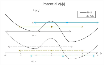
Figure 1: The upper panel is the dSdS potential (both minima are dS-like), the lower panel is the dSAdS potential (one minimum is dS-like, the other is AdS-like). Lengths of the arrow lines represent the initial amplitude of $\phi$. The brown, grey, blue colored lines and dotted lines correspond to different sets in our simulations, i.e.the 1st, 2nd and 3rd set, respectively.

In an effective theory, the string landscape might correspond to a complex and rugged potential. However, for simplicity, we set the potential $\sim\phi^{2}$ around its minima , which are separated by a fourth-order polynomial barrier,

$$V\left(\phi\right)=\left\{\begin{aligned} &\frac{1}{2}m_{1}^{2}{\left(\phi-\phi_{1}\right)}^{2}+V_{1},&\phi<\phi_{1},\\ &\lambda\left(\phi^{2}+{1\over 2\lambda}\right)^{2}-\phi^{3}-{1\over 4\lambda}+V_{1},\quad&\quad\phi_{1}\leq\phi\leq\phi_{2},\\ &\frac{1}{2}m_{2}^{2}{\left(\phi-\phi_{2}\right)}^{2}+V_{2},&\phi_{2}<\phi,\end{aligned}\right.$$ (1)

see Fig.1. The minima of the fourth-order polynomial are at $\phi_{1}=0$ and $\phi_{2}=\frac{3+\sqrt{9-32\lambda}}{8\lambda}$ $(\lambda<\frac{9}{32})$, respectively, at which the potential is differentiable. In the simulation, we will fix $m_{1}^{2}=m_{2}^{2}=0.2$ and $\lambda=0.2375$.

The initial inhomogeneity of the scalar field $\phi$ is regarded as

$$\left.\phi\right|_{t=0}=\phi_{0}+\Delta\phi\sum_{\vec{x}=x,y,z}\cos\left(\frac{2\pi\vec{x}}{L}\right),$$ (2)

similar to that in Refs.East et al. (2016); Clough et al. (2017), where $\vec{x}$ is the spatial coordinate, $\Delta\phi$ is the amplitude of initial inhomogeneity, while the length of the simulated cubic region is $L=4$. The initial expansion rates for the dSdS and dSAdS scenarios are $H_{init}=0.7,0.6$ respectively, corresponding to Hubble radii $H^{-1}=1.43,1.67<L$, i.e. the initial scale of inhomogeneity is superhorizon.

In light of the potential in (1), we classify the scenarios simulated as dSdS (both vacua are dS-like) and dSAdS (one is dS-like and the other is AdS-like). We will consider simulations of 3 cases (for dSdS and dSAdS, respectively), with $\Delta\phi=0.7$ but different average field value $\phi_{0}=0.2,1.0,1.7$ for dSdS ($\phi_{0}=0.3,1.0,2.0$ for dSAdS), where $\phi_{0}=0.2,1.7(0.3,2.0)$ indicates that the initial distribution of $\phi$ is biased towards one of the vacua, see Fig.1. Here, the inhomogeneity considered clearly exceeds the perturbative level. However, during the very early stage of the Universe, the initial inhomogeneity might arise from large quantum fluctuations with $\Delta\phi\simeq H$, where $H\sim\mathcal{O}(1)$. In addition, the String landscape conjectures bounds on the scalar field excursion, e.g., in Agrawal et al. (2018); Ooguri and Vafa (2007) $|\Delta\phi|<\mathcal{O}(1)$, which is also consistent with our model.

Appendix A shows a brief review on NR based on BSSN Baumgarte and Shapiro (1998); Shibata and Nakamura (1995) and the symbols and conventions in our paper. We set the initial values of BSSN parameters as $\widetilde{\gamma}_{ij}=\delta_{ij}$, $\widetilde{A}_{ij}=0$, and the initial spatial expansion uniform ($K=const.<0$) and $\dot{\phi}=0$, which naturally satisfy the momentum constraints. The Hamiltonian constraint is then solved by relaxing $\chi$ from the initial value $\chi=1$ with the parabolic equation ${\partial}_{t}\chi=\mathcal{H}$. This equation is iterated until it converges (suggesting ${\partial}_{t}\chi=\mathcal{H}=0$). The resolution of the simulation is $32\times 32\times 32$ along the x,y,z axes on the coarsest level with up to 3 levels of AMR regridding.

III Results and analysis

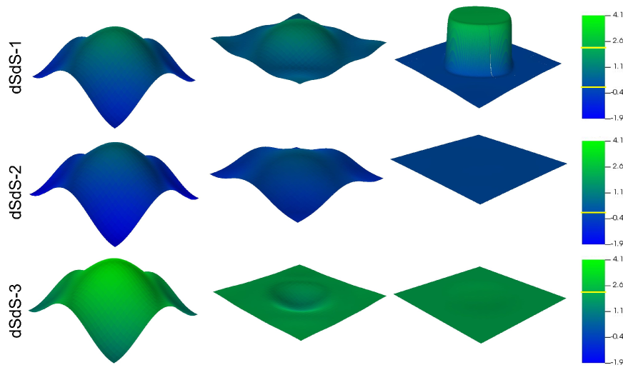
Figure 2: Results of $\phi$ at $x-y$ slices at different timesteps (proceeding from left to right) for dSdS-1,2,3. The colorbar and the elevation height show the value of $\phi$. The yellow line on the colorbar marks the converged values of $\phi$.

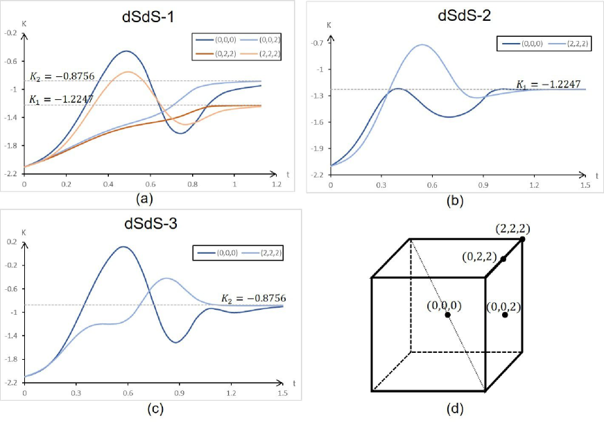
Figure 3: The evolution of $K$ for dSdS-1,2,3. $K_{1}$ and $K_{2}$ correspond to the local Hubble rate at $\phi_{1}$ and $\phi_{2}$, respectively (noting both $V(\phi_{1}),V(\phi_{2})>0$ for dSdS in Fig.1). (d) shows the labelling of the positions in (a)(b)(c). These positions are at the bulk (center) of the vacua or where these regions intersect the simulation boundary, and best capture the physics of corresponding vacua.

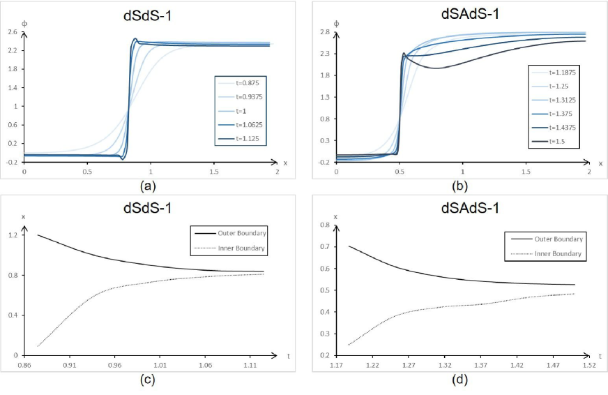
Figure 4: Upper row: the value of $\phi$ along the $x$-axis, showing the different vacua regions with $\phi=2.2$ and $\phi=0$ separated by a bubble wall. The darker lines show the field configurations for later time. Second row: positions of the inner and outer boundaries of the bubble wall. It is clear that the width of the bubble wall in comoving coordinates shrinks with time, which indicates that the position of the bubble wall freezes.

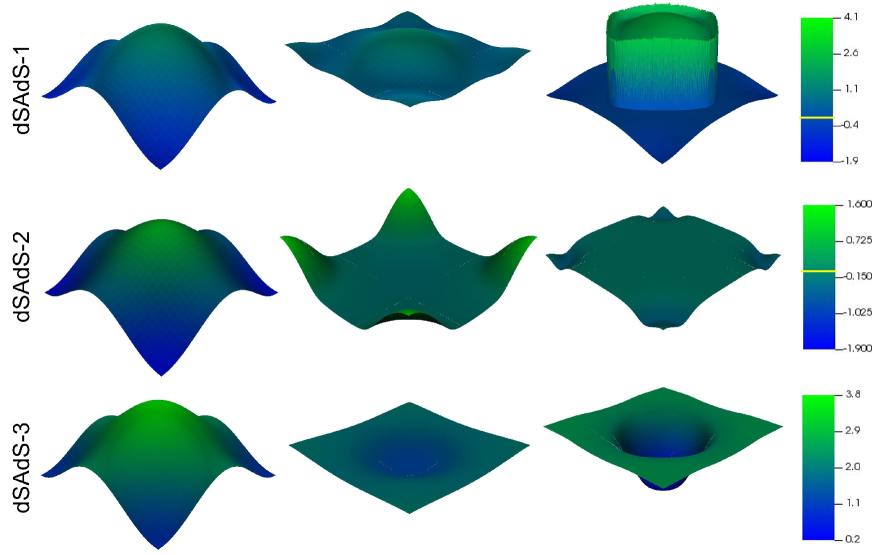
Figure 5: Results of $\phi$ at $x-y$ slices at different timesteps (proceeding from left to right) for dSAdS-1,2,3. The colorbar and the elevation height show the value of $\phi$. The yellow line on the colorbar marks the converged values of $\phi$.

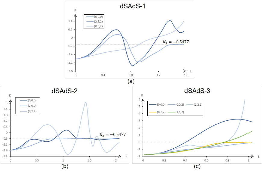
Figure 6: The evolution of $K$ for dSAdS-1,2,3. $K_{3}$ corresponds to the local Hubble rate at $\phi_{1}$ (noting $V(\phi_{1})>0$ and $V(\phi_{2})<0$ for dSAdS in Fig.1). The positions are labelled in accordance with Fig.3 (d).

We will perform the NR simulations with modified GRChombo package to investigate how the field populates the landscape in Fig.1 in an inhomogeneous Universe that is initially expanding.

As a contrast, we first consider a landscape consisting of only dS vacua. We show the evolutions of $\phi$ at certain regions for dSdS-1,2,3 in Fig.2. The field initially underwent a rapidly oscillating phase. However, eventually, for dSdS-1 the field in different spatial region will separate into different vacua, and the dS bubbles come into being with clear boundries, while for dSdS-2,3, the overall region will be in a nearly homogeneous dS expansion.

The Hubble rate at a local homogeneous region is

$$H_{local}=\lim\limits_{V\rightarrow 0}\sqrt{{1\over V}\int{\rho(\phi)\over 3}dV}=-{K\over 3},$$ (3)

In Fig.3, for dSdS-1, the local Hubble rate will be $H_{local}=({V(\phi_{1,2})\over 3})^{1/2}$, i.e. that at different vacua $\phi_{1}$ and $\phi_{2}$, respectively, and for dSdS-2,3, $H_{local}$ will be identical eventually at all region, i.e. a homogeneous dS expansion. The result is consistent with Fig.2.

In our simulation results for dSdS-1, eventually the dS bubbles will emerge in high-energy dS background. It is well-known that if the radius of the bubble is larger than the Hubble radius of the background, $r\geqslant H^{-1}$, the bubble wall will expand with the background. In Fig.2, we see that the position of the bubble wall is frozen, suggesting that the dS bubble is in fact expanding with the background. However, the condition $r>1/H$ is not strictly satisfied in our simulation, the Hubble length $H^{-1}$ of background in dSdS-1 is 2.45, which is comparable but not less than the the radius $r\simeq 1$ of bubble.

It is more interesting to investigate the dSAdS landscape in Fig.1. We show the evolutions of $\phi$ at different regions for dSAdS-1,2,3 in Fig.5. Results show that dSAdS behaved similarly to dSdS only at the initial stage of the evolution.

It is significant to check the local expansion rate. In Fig.6, for dSAdS-1, some regions eventually converged to $H_{local}=const.>0$ (the dS expansion), while other regions have $H_{local}<0$. In Fig.7, these contracting AdS regions will always collapse. Ref.Felder et al. (2002) investigated a homogeneous case with $V_{min}<0$ and showed the diverging property of $H$ once it crosses to the negative side, which indicates the final fate of the AdS bubbles in our simulation. For dSAdS-2, after the initial oscillation, the overall region will have a nearly homogeneous dS expansion, except for a few smaller AdS bubbles, see Fig.7. Thus our results show that the expanding dS regions may be present eventually, even if the AdS vacua exist. For dSAdS-3, the story is different. Due to the rapid collapse of the AdS spacetime, the numerical code is unable to evolve the system after the collapsing regions run into “singularities” somewhere. In Fig.7, we see that some regions with $K<0$ are left at the end of the simulation. However, these regions cannot evolve to a stable dS spacetime, because the profile of $\phi$ has crossed the potential barrier and fallen in the range of the AdS minima, see the 3rd row of Fig.5. The corresponding AdS vacua will eventually stop the expansion of these regions and convert them into collapsing spacetime. We thus conclude that the overall region will eventually be AdS-like, resulting in an inhomogeneous collapse.

In our simulation result for dSAdS-1, see Fig.4, eventually the position of the bubble wall is frozen, suggesting that the wall of AdS bubble is expanding with bakground, so such AdS bubbles correspond to the separated Universes, but the spacetime inside AdS bubbles is contracting (confirming the argument of Ref.Abbott and Coleman (1985)). The radius of AdS bubbles is approximately $r<1/H\simeq 5.48$. Again, as in dSdS-1, the condition $r>1/H$ is not satisfied. The contracting AdS bubble might be relevant to our Universe Piao (2004, 2009); Johnson and Lehners (2012); Garriga et al. (2013), if a nonsingular bounce happened, which might explain the large-scale CMB power deficit Piao et al. (2004); Liu et al. (2013); Cai et al. (2018). While in dSAdS-2, the AdS bubbles have its radius $r\ll 1/H$, which (to observers outside the bubbles) will then collapse into black holes, see also Blanco-Pillado et al. (2020); Garriga et al. (2016).

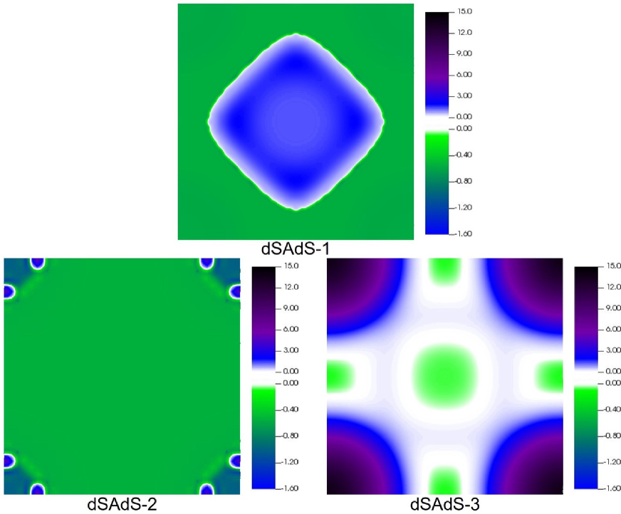
Figure 7: The values of $K$ for dSAdS-1,2,3 at final timesteps. There are two sets of colorbars: the upper colorbar shows the value of $K$ for $K>0$ (the contracting region), while the lower colorbar shows that for $K<0$ (the expanding region), the two regions are seperated by walls where $K=0$ colored in white.

IV Conclusions

It is usually speculated that the primordial Universe is highly inhomogeneous, i.e. the scalar field or spacetime metric has large inhomogeneities. How the landscape is populated in an inhomogeneous Universe is still a significant question.

In an inhomogeneous Universe that is initially expanding, we perform the 3+1D Numerical Relativity simulations for the evolution of a scalar field in the simplified landscape in Fig.1, and investigated how the field populates such a landscape. The simulation results showed that eventually, either the overall region is in a nearly homogeneous dS expansion (for dSAdS, however, a few smaller regions corresponding to AdS bubbles collapsed into black holes), or the whole region is inhomogeneously collapsing, or the field in different spatial region separates into different vacua, so that expanding dS and AdS bubbles (the bubble wall is expanding but the spacetime inside AdS bubbles is contracting) come into being with clear bounderies.

It is noted that the initial high inhomogeneities seem to amplify the probability that different regions of Universe arrive at different vacua. Also, the bubble wall expand with the background seems to not require that the bubble radius must be strictly larger than the Hubble radius. Though we perform the simulation in a simplified landscape, our results have captured relevant physics.

The theory of inflation as a paradigm of early universe indicates an existence of a dS or quasi-dS phase of the Universe. Studies on the String landscape had attempted to answer the questions of whether a dS vacua is permitted in String theory and, if so, how can dS vacua be constructed. On the other hand, the initial conditions of the Universe is not necessarily (in fact, unlikely) homogeneous. Here, we discuss the questions of how in a highly inhomogeneous Universe (where the dS vacua is not yet populated) a patch of spacetime evolves into the dS vacua, if they exist. We showed that the “islands” of dS spacetime can naturally emerge depending on the initial conditions of the field configuration. Thus we actually suggested the possibility for the appearance and existence of local dS spacetime that corresponds to our Universe.

An interesting issue that follows is what signals would we “see” if our Universe indeed went through such an inhomogeneous evolution before or during inflation?

Acknowledgment PXL would like to thank Gen Ye, Hao-Hao Li, Hao-Yang Liu for helpful discussions. We also acknowledge the use of the package GRChombo and VisIt. This work is supported by NSFC, Nos.12075246, 11690021, and also UCAS Undergraduate Innovative Practice Project.

Appendix A A brief review on NR and BSSN formalism

In the context of 3+1 decomposition of NR, the metric is

$$g_{00}=-{\alpha}^{2}+{\beta}_{i}{\beta}^{i},\qquad g_{0i}={\beta}_{i},\qquad g_{ij}={\gamma}_{ij},$$ (4)

where $\alpha$ is the lapse parameter, ${\beta}^{i}$ the shift vector and ${\gamma}_{ij}$ the spatial metric. In order to formulate the evolution of spacetime and the “matter” inside as a well-posed Cauchy problem, the system of partial differential equations should be explicitly written in a hyperbolic form. According to BSSN Baumgarte and Shapiro (1998); Shibata and Nakamura (1995), the evolution equation are

$${\partial}_{t}\chi=\frac{2}{3}\alpha\chi K-\frac{2}{3}\chi{\partial}_{k}{\beta}^{k}+{\beta}^{k}{\partial}_{t}\chi,$$ (5)

$${\partial}_{t}\widetilde{\gamma}_{ij}=-2\alpha\widetilde{A}_{ij}+\widetilde{\gamma}_{ik}{\partial}_{j}{\beta}^{k}+\widetilde{\gamma}_{jk}{\partial}_{i}{\beta}^{k}-\frac{2}{3}\widetilde{\gamma}_{ij}{\partial}_{k}{\beta}^{k}+{\beta}^{k}{\partial}_{k}\widetilde{\gamma}_{ij},$$ (6)

$${\partial}_{t}K=-\widetilde{\gamma}^{ij}D_{i}D_{j}\alpha+\alpha\left(\widetilde{A}_{ij}\widetilde{A}^{ij}+\frac{1}{3}K^{2}\right)+{\beta}^{i}{\partial}_{i}K+4\pi G\alpha\left(\rho+S\right),$$ (7)

$${\partial}_{t}\widetilde{A}_{ij} =\chi{\left[-D_{i}D_{j}\alpha+\alpha\left(R_{ij}-8\pi\alpha S_{ij}\right)\right]}^{TF}+\alpha\left(K\widetilde{A}_{ij}-2\widetilde{A}_{il}\widetilde{A}\right)$$ (8)

$$+\widetilde{A}_{ik}{\partial}_{j}{\beta}^{k}+\widetilde{A}_{jk}{\partial}_{i}{\beta}^{k}-\frac{2}{3}\widetilde{A}_{ij}{\partial}_{k}{\beta}^{k}+{\beta}^{k}{\partial}_{k}\widetilde{A}_{ij},$$

$${\partial}_{t}\widetilde{\Gamma}^{i} =-2\widetilde{A}^{ij}{\partial}_{j}\alpha+2\alpha\left(\widetilde{\Gamma}^{i}_{jk}\widetilde{A}^{jk}-\frac{2}{3}\widetilde{\gamma}^{ij}{\partial}_{j}K-\frac{3}{2\chi}\widetilde{A}^{ij}{\partial}_{j}\chi\right)+{\beta}^{k}{\partial}_{k}\widetilde{\Gamma}^{i}+\widetilde{\gamma}^{jk}{\partial}_{j}{\partial}_{k}{\beta}^{i}$$ (9)

$$+\frac{1}{3}\widetilde{\gamma}^{ij}{\partial}_{j}{\partial}_{k}{\beta}^{k}+\frac{2}{3}\widetilde{\Gamma}^{i}{\partial}_{k}{\beta}^{k}-\widetilde{\Gamma}^{k}{\partial}_{k}{\beta}^{i}-16\pi G\alpha\widetilde{\gamma}^{ij}S_{j},$$

where the tilde represent the conformal quantities $\widetilde{\gamma}_{ij}=\chi\gamma_{ij}$, $\widetilde{\Gamma}^{i}\equiv\widetilde{\gamma}^{jk}\widetilde{\Gamma}^{i}_{jk}$ and $K$ is the extrinsic curvature. The Hamiltonian and momentum constraints are

$$\mathcal{H}=\widetilde{D}^{2}\chi-\frac{5}{4\chi}\widetilde{\gamma}^{ij}\widetilde{D}_{i}\chi\widetilde{D}_{j}\chi+\frac{\chi\widetilde{R}}{2}+\frac{K^{2}}{3}-\frac{1}{2}\widetilde{A}^{ij}\widetilde{A}_{ij}-8\pi G\rho=0,$$ (10)

$$\mathcal{M}^{i}=\widetilde{D}_{j}\widetilde{A}^{ij}-\frac{3}{2\chi}\widetilde{A}^{ij}\widetilde{D}_{j}\chi-\frac{2}{3}\widetilde{\gamma}^{ij}\widetilde{D}_{j}K-8\pi G\Pi\widetilde{\gamma}^{ij}{\partial}_{j}\phi=0.$$ (11)

The Klein-Gordon equation of canonical scalar field $\phi$ is $\Box\phi=-V^{\prime}$. According to BSSN, it is rewritten as Clough et al. (2015) (with the momentum conjugate $\Pi=\frac{1}{\alpha}\left({\partial}_{t}\phi-\beta^{i}{\partial}_{i}\phi\right)$)

$${\partial}_{t}\Pi=\alpha\left(K\Pi-\Gamma^{k}{\partial}_{k}\phi-V^{\prime}\right)+\alpha{\partial}_{i}\partial^{i}\phi+{\partial}_{i}\phi\partial^{i}\alpha+\beta^{i}{\partial}_{i}\Pi.$$ (12)

The gauge conditions in our simulations are the 1+log slicing and the Eulerian gauge,

$${\partial}_{t}\alpha=-2\alpha K+\beta^{i}{\partial}_{i}\alpha,\quad\beta^{i}=0,$$ (13)

, see e.g.Alcubierre (2008); Baumgarte and Shapiro (2010); Gourgoulhon (2007); Lehner (2001) for details.

Appendix B On Hamiltonian constraint and convergence test

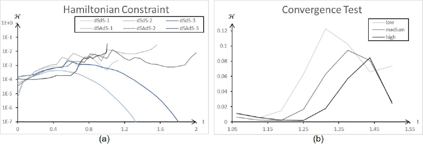
Figure 8: (a): The box-averaged $L_{2}$-norm of the Hamiltonian constraint $\mathcal{H}$. Due to the fact that the Hamiltonian of different points can cross $H=0$, a fraction Hamiltonian violation cannot be globally defined. Thus, with the data yielding the average $H\sim O\left(1\right)$, we instead keep the absolute constraint violation under $10^{-2}$. (b): A convergence test with different grid resolutions. The presented results shows the Hamiltonian violation of case dSAdS-1 when the bubble wall formed. Higher resolution yields higher pricision at the start of the bubble wall formation, afterwards, the results under meduim and high resolutions start to converge.

References

- Guth (1981) A. H. Guth, Phys. Rev. D 23, 347 (1981).
- Linde (1982) A. D. Linde, Phys. Lett. B 108, 389 (1982).
- Albrecht and Steinhardt (1982) A. Albrecht and P. J. Steinhardt, Phys. Rev. Lett. 48, 1220 (1982).
- Starobinsky (1980) A. A. Starobinsky, Phys. Lett. B 91, 99 (1980).
- Sato (1981) K. Sato, Mon. Not. Roy. Astron. Soc. 195, 467 (1981).
- Fang (1980) L. Z. Fang, Phys. Lett. B 95, 154 (1980).
- Bousso and Polchinski (2000) R. Bousso and J. Polchinski, JHEP 06, 006 (2000), eprint hep-th/0004134.
- Susskind (2003) L. Susskind, pp. 247–266 (2003), eprint hep-th/0302219.
- Ooguri and Vafa (2007) H. Ooguri and C. Vafa, Nucl. Phys. B 766, 21 (2007), eprint hep-th/0605264.
- Obied et al. (2018) G. Obied, H. Ooguri, L. Spodyneiko, and C. Vafa (2018), eprint 1806.08362.
- Danielsson et al. (2009) U. H. Danielsson, S. S. Haque, G. Shiu, and T. Van Riet, JHEP 09, 114 (2009), eprint 0907.2041.
- Piao (2004) Y.-S. Piao, Phys. Rev. D 70, 101302 (2004), eprint hep-th/0407258.
- Piao and Zhang (2005) Y.-S. Piao and Y.-Z. Zhang, Nucl. Phys. B 725, 265 (2005), eprint gr-qc/0407027.
- Garriga et al. (2013) J. Garriga, A. Vilenkin, and J. Zhang, JCAP 11, 055 (2013), eprint 1309.2847.
- Blanco-Pillado et al. (2020) J. J. Blanco-Pillado, H. Deng, and A. Vilenkin, JCAP 05, 014 (2020), eprint 1909.00068.
- Li et al. (2020) H.-H. Li, G. Ye, Y. Cai, and Y.-S. Piao, Phys. Rev. D 101, 063527 (2020), eprint 1911.06148.
- Ye and Piao (2020a) G. Ye and Y.-S. Piao, Phys. Rev. D 101, 083507 (2020a), eprint 2001.02451.
- Ye and Piao (2020b) G. Ye and Y.-S. Piao, Phys. Rev. D 102, 083523 (2020b), eprint 2008.10832.
- Coleman (1977) S. R. Coleman, Phys. Rev. D 15, 2929 (1977), [Erratum: Phys.Rev.D 16, 1248 (1977)].
- Coleman and De Luccia (1980) S. R. Coleman and F. De Luccia, Phys. Rev. D 21, 3305 (1980).
- Blau et al. (1987) S. K. Blau, E. I. Guendelman, and A. H. Guth, Phys. Rev. D 35, 1747 (1987).
- Lee and Weinberg (1987) K.-M. Lee and E. J. Weinberg, Phys. Rev. D 36, 1088 (1987).
- Linde (1992) A. D. Linde, Nucl. Phys. B 372, 421 (1992), eprint hep-th/9110037.
- Easther et al. (2009) R. Easther, J. T. Giblin, Jr, L. Hui, and E. A. Lim, Phys. Rev. D 80, 123519 (2009), eprint 0907.3234.
- Brown and Dahlen (2011) A. R. Brown and A. Dahlen, Phys. Rev. Lett. 107, 171301 (2011), eprint 1108.0119.
- Braden et al. (2019) J. Braden, M. C. Johnson, H. V. Peiris, A. Pontzen, and S. Weinfurtner, Phys. Rev. Lett. 123, 031601 (2019), eprint 1806.06069.
- Blanco-Pillado et al. (2019) J. J. Blanco-Pillado, H. Deng, and A. Vilenkin, JCAP 12, 001 (2019), eprint 1906.09657.
- Huang and Ford (2020) H. Huang and L. H. Ford (2020), eprint 2005.08355.
- Wang (2019) S.-J. Wang, Phys. Rev. D 100, 096019 (2019), eprint 1909.11196.
- Li and Wang (2009) M. Li and Y. Wang, JCAP 07, 033 (2009), eprint 0903.2123.
- Li et al. (2009) S. Li, Y. Liu, and Y.-S. Piao, Phys. Rev. D 80, 123535 (2009), eprint 0906.3608.
- Cai et al. (2021) T. Cai, J. Jiang, and Y. Wang (2021), eprint 2110.05268.
- Lehner and Pretorius (2014) L. Lehner and F. Pretorius, Ann. Rev. Astron. Astrophys. 52, 661 (2014), eprint 1405.4840.
- Cardoso et al. (2015) V. Cardoso, L. Gualtieri, C. Herdeiro, and U. Sperhake, Living Rev. Relativity 18, 1 (2015), eprint 1409.0014.
- Palenzuela (2020) C. Palenzuela, Front. Astron. Space Sci. 7, 58 (2020), eprint 2008.12931.
- Giblin et al. (2016) J. T. Giblin, J. B. Mertens, and G. D. Starkman, Phys. Rev. Lett. 116, 251301 (2016), eprint 1511.01105.
- Macpherson et al. (2017) H. J. Macpherson, P. D. Lasky, and D. J. Price, Phys. Rev. D 95, 064028 (2017), eprint 1611.05447.
- Macpherson et al. (2019) H. J. Macpherson, D. J. Price, and P. D. Lasky, Phys. Rev. D 99, 063522 (2019), eprint 1807.01711.
- Giblin and Tishue (2019) J. T. Giblin and A. J. Tishue, Phys. Rev. D 100, 063543 (2019), eprint 1907.10601.
- Kou et al. (2021) X.-X. Kou, C. Tian, and S.-Y. Zhou, Class. Quant. Grav. 38, 045005 (2021), eprint 1912.09658.
- East et al. (2016) W. E. East, M. Kleban, A. Linde, and L. Senatore, JCAP 09, 010 (2016), eprint 1511.05143.
- Clough et al. (2017) K. Clough, E. A. Lim, B. S. DiNunno, W. Fischler, R. Flauger, and S. Paban, JCAP 09, 025 (2017), eprint 1608.04408.
- Clough et al. (2018) K. Clough, R. Flauger, and E. A. Lim, JCAP 05, 065 (2018), eprint 1712.07352.
- Aurrekoetxea et al. (2020) J. C. Aurrekoetxea, K. Clough, R. Flauger, and E. A. Lim, JCAP 05, 030 (2020), eprint 1910.12547.
- Joana and Clesse (2021) C. Joana and S. Clesse, Phys. Rev. D 103, 083501 (2021), eprint 2011.12190.
- Johnson et al. (2012) M. C. Johnson, H. V. Peiris, and L. Lehner, Phys. Rev. D 85, 083516 (2012), eprint 1112.4487.
- Wainwright et al. (2014a) C. L. Wainwright, M. C. Johnson, H. V. Peiris, A. Aguirre, L. Lehner, and S. L. Liebling, JCAP 03, 030 (2014a), eprint 1312.1357.
- Wainwright et al. (2014b) C. L. Wainwright, M. C. Johnson, A. Aguirre, and H. V. Peiris, JCAP 10, 024 (2014b), eprint 1407.2950.
- Johnson et al. (2016) M. C. Johnson, C. L. Wainwright, A. Aguirre, and H. V. Peiris, JCAP 07, 020 (2016), eprint 1508.03641.
- Nazari et al. (2021) Z. Nazari, M. Cicoli, K. Clough, and F. Muia, JCAP 05, 027 (2021), eprint 2010.05933.
- de Jong et al. (2021) E. de Jong, J. C. Aurrekoetxea, and E. A. Lim (2021), eprint 2109.04896.
- Clough et al. (2015) K. Clough, P. Figueras, H. Finkel, M. Kunesch, E. A. Lim, and S. Tunyasuvunakool, Class. Quant. Grav. 32, 245011 (2015), eprint 1503.03436.
- Agrawal et al. (2018) P. Agrawal, G. Obied, P. J. Steinhardt, and C. Vafa, Phys. Lett. B 784, 271 (2018), eprint 1806.09718.
- Baumgarte and Shapiro (1998) T. W. Baumgarte and S. L. Shapiro, Phys. Rev. D 59, 024007 (1998), eprint gr-qc/9810065.
- Shibata and Nakamura (1995) M. Shibata and T. Nakamura, Phys. Rev. D 52, 5428 (1995).
- Felder et al. (2002) G. N. Felder, A. V. Frolov, L. Kofman, and A. D. Linde, Phys. Rev. D 66, 023507 (2002), eprint hep-th/0202017.
- Abbott and Coleman (1985) L. F. Abbott and S. R. Coleman, Nucl. Phys. B 259, 170 (1985).
- Piao (2009) Y.-S. Piao, Phys. Lett. B 677, 1 (2009), eprint 0901.2644.
- Johnson and Lehners (2012) M. C. Johnson and J.-L. Lehners, Phys. Rev. D 85, 103509 (2012), eprint 1112.3360.
- Piao et al. (2004) Y.-S. Piao, B. Feng, and X.-m. Zhang, Phys. Rev. D 69, 103520 (2004), eprint hep-th/0310206.
- Liu et al. (2013) Z.-G. Liu, Z.-K. Guo, and Y.-S. Piao, Phys. Rev. D 88, 063539 (2013), eprint 1304.6527.
- Cai et al. (2018) Y. Cai, Y.-T. Wang, J.-Y. Zhao, and Y.-S. Piao, Phys. Rev. D 97, 103535 (2018), eprint 1709.07464.
- Garriga et al. (2016) J. Garriga, A. Vilenkin, and J. Zhang, JCAP 02, 064 (2016), eprint 1512.01819.
- Alcubierre (2008) M. Alcubierre, Introduction to 3+ 1 numerical relativity, vol. 140 (Oxford University Press, 2008).
- Baumgarte and Shapiro (2010) T. W. Baumgarte and S. L. Shapiro, Numerical relativity: solving Einstein’s equations on the computer (Cambridge University Press, 2010).
- Gourgoulhon (2007) E. Gourgoulhon (2007), eprint gr-qc/0703035.
- Lehner (2001) L. Lehner, Class. Quant. Grav. 18, R25 (2001), eprint gr-qc/0106072.