Cosmological constraints on the gravitational constant

Abstract

We study the variation of the gravitational constant on cosmological scales in scalar-tensor theories of gravity. We focus on the simplest models of scalar-tensor theories with a coupling to the Ricci scalar of the form $F(\sigma)=N_{\rm pl}^{2}+\xi\sigma^{2}$, such as extended Jordan-Brans-Dicke ($N_{\rm pl}=0$), or a non-minimally coupled scalar field with $N_{\rm pl}=M_{\rm pl}$, which permits the gravitational constant to vary self-consistently in time and space. In addition, we allow the effective gravitational constant on cosmological scales to differ from the Newton’s measured constant $G$, i.e. $G_{\rm eff}(z=0)=G\left(1+\Delta\right)^{2}$. We study the impact of this imbalance $\Delta$ jointly with the coupling $\xi$ into anisotropies of the cosmic microwave background and matter power spectrum at low-redshift. Combining the information from Planck 2018 CMB temperature, polarization and lensing, together with a compilation of BAO measurements from the release DR12 of the Baryon Oscillation Spectroscopic Survey (BOSS), we constrain the imbalance to $\Delta=-0.022\pm 0.023$ (68% CL) and the coupling parameter to $10^{3}\,\xi<0.82$ (95% CL) for Jordan-Brans-Dicke and for a non-minimally coupled scalar field with $F(\sigma)=M^{2}_{\rm pl}+\xi\sigma^{2}$ we constrain the imbalance to $\Delta>-0.018$ ($<0.021$) and the coupling parameter to $\xi<0.089$ ($\xi>-0.041$) both at 95% CL. With current data, we observe that the degeneracy between $\Delta$, the coupling $\xi$ to the Ricci scalar, and $H_{0}$ allows for a larger value of the Hubble constant increasing the consistency between the distance-ladder measurement of the Hubble constant from supernovae type Ia by the SH0ES team and its value inferred by CMB data. We also study how future cosmological observations can constrain the gravitational Newton’s constant. Future data such as the combination of CMB anisotropies from LiteBIRD and CMB-S4, and large-scale structures galaxy clustering from DESI and galaxy shear from LSST reduce the uncertainty in $\Delta$ to $\sigma(\Delta)\simeq 0.004$.

1 Introduction

The Universe is a unique and peculiar laboratory to test fundamental physical laws and possible clues for physics beyond the current standard understanding. In particular, the exciting possibility that fundamental constants [1] could vary in time, which has long been proposed by Dirac [2], can be tested through cosmological observations at higher and higher precision. Cosmology can indeed uniquely probe lengths and/or timescales otherwise inaccessible on ground and from Solar System experiments.

Among the different fundamental constants, Newton’s constant remains the one with the largest relative uncertainty from laboratory measurements. According to CODATA, the value of Newton’s constant G is $6.67430(15)\times 10^{-8}$ cm³ g^-1 s^-2 with a relative uncertainty of $2.2\times 10^{-5}$.

General Relativity (GR) has been tested exquisitely in the Solar System and on extra-galactic systems [3] setting observational challenges for the theories alternative to Einstein gravity. As Solar System tests on parameterized post Newtonian (PPN) parameters we quote the time dilation due to the effect of the Sun’s gravitational field measured very accurately using the signal from Cassini satellite giving a constraint $\gamma_{\rm PN}=\left(2.1\pm 2.3\right)\times 10^{-5}$ [4] and the perihelion shift of Mercury $\beta_{\rm PN}-1=\left(-4.1\pm 7.8\right)\times 10^{-5}$ [5], assuming the Cassini bound. Lunar laser ranging data provide a tight constraint on the time variation of the gravitational constant $\dot{G}/G=\left(2\pm 7\right)\times 10^{-13}$ yr^-1 [6]. Other extra-galactic constraints on the time-variation of $G$ come from stellar [7, 8, 9] and pulsar timing [10].

As previously stated, cosmological observations can constrain the gravitational constant at totally different scale and redshift. The primordial abundances of light elements allow to constrain gravitational constant during Big Bang Nucleosynthesis (BBN) based on the modified ratio of the expansion rate and a given prior value/range of the baryon density $\omega_{\rm b}$ [11, 12, 13, 14, 15, 16, 17]. Current measurements of the primordial abundances of helium and deuterium constrain $0.04<(\delta G/G)<-0.08$ at 95% CL [17] at nucleosynthesis by assuming $\omega_{\rm b}=0.02236\pm 0.00030$ at 68% CL [18]. A different value of the gravitational constant in the Einstein equations can be interpreted as a change in the background expansion history and distance measurements [19, 20, 21, 22, 23, 24], and in recombination for cosmic microwave background (CMB) physics [25, 26, 27].

Scalar-tensor theories of gravity, with a scalar field non-minimally coupled to gravity, modify GR by dynamically determining the value of the gravitational constant and can accommodate self-consistently space and time variation of the gravitational constant. The most recent Planck 2018 and baryon acoustic oscillation (BAO) data constrain the variation of the gravitational constant with respect to the radiation era to be smaller than 3% at 95% CL [28] by assuming adiabatic initial condition for scalar fluctuations [29] and the effective gravitational constant at present corresponding to the Newton’s measured constant (see [19, 20, 30, 31, 32] for previous constraints). In these scalar-tensor theories of gravity, the cosmological constraints on the time variation of the gravitational constant can be tighter than those from the Lunar Laser ranging.

This paper wants to go further and study in detail the impact of an imbalance $\Delta$ between the effective gravitational constant at present and measured value of the Newton’s constant, defined as $G_{\rm eff}(z=0)=G(1+\Delta)^{2}$, jointly with the coupling to the curvature in simple scalar-tensor theories where the gravitational constant can vary self consistently in space and time. We will explore the impact of $\Delta\neq 0$ on the CMB anisotropies and matter power spectrum at low redshift calculating the joint constraints on $\Delta$ and on the coupling to the Ricci scalar with publicly available data and future cosmological observations.

It is important to stress that these minimal scalar-tensor theories are not only workhorse models to study how cosmology can constrain gravity on large scales, but are also of great current interest since alleviate the existing tension [33, 34] between distance-ladder measurement of the Hubble constant from supernovae type Ia by the SH0ES team and its value inferred by CMB data. Moreover the mismatch between different values of the Hubble constant can be reduced assuming a late-time transition of the effective gravitational constant [35, 36].

The paper is organized as follows. After this introduction, we describe the implementation of the variation of the gravitational constant in the context of scalar-tensor theories in Section 2. In Section 3 we describe the datasets and prior considered and in Section 4 we discuss our results in light of CMB and BAO data. We present the Fisher methodology for CMB and LSS for our science forecasts and the results in Section 5. In Section 6 we draw our conclusions. In App. A-B, we collect all the tables and triangle plots with the constraints on the cosmological parameters obtained with our MCMC analysis.

2 Varying $G$ within minimal scalar-tensor theory

In this paper, we use a scalar field non-minimally coupled (NMC) to the Ricci scalar as the simplest scalar-tensor theory of gravity [37, 38] with which we test deviations from GR and constrain the variation of the effective gravitational constant $G_{\rm eff}$ from cosmology, as previously done in [39, 40, 41, 42, 43, 30, 31, 44, 45, 32, 46, 47, 48, 28, 49, 50, 51].

By using NMC scalar fields, we have a self-consistent way of modifying both the background dynamics of the universe and that of the perturbations accurately for both early- and late-time probes. In order to do so, we consider the NMC theory described by

$$S=\int\mathrm{d}^{4}x\sqrt{-g}\left[\frac{F(\sigma)}{2}R-\frac{g^{\mu\nu}}{2}\partial_{\mu}\sigma\partial_{\nu}\sigma-V(\sigma)+{\cal L}_{m}\right]\,,$$ (2.1)

where $\sigma$ is a scalar field, $F(\sigma)=N_{\rm pl}^{2}+\xi\sigma^{2}$, $R$ is the Ricci scalar, and ${\cal L}_{m}$ is the Lagrangian density for matter fields. We restrict ourselves to a potential of the type $V(\sigma)\propto F^{2}(\sigma)$ [52, 53] in which the scalar field is effectively massless and the effective gravitational constant $G_{\rm eff}$ between two test masses is [54]

$$G_{\rm eff}(z=0)=\frac{1}{8\pi F_{0}}\frac{2F_{0}+4F_{0,\sigma}^{2}}{2F_{0}+3F_{0,\sigma}^{2}}\,.$$ (2.2)

We define also the gravitational constant entering in the NMC background equations $G_{\rm N}=(8\pi F)^{-1}$. For the full set of background equations and linear cosmological perturbations in NMC scalar-tensor models, we refer the interested reader to Refs. [54, 30, 32]. In this paper, we allow an imbalance $\Delta$ between $G_{\rm eff}(z=0)$ and $G$

$$G_{\rm eff}(z=0)=G\left(1+\Delta\right)^{2}\,,$$ (2.3)

which was fixed to zero in many previous studies [30, 31, 32, 28].

We consider the following three cases of the model: induced gravity (IG) described by $N_{\rm pl}=0$ and $\xi>0$, a conformally coupled scalar field (CC) described by $N_{\rm pl}=M_{\rm pl}$ and $\xi=-1/6$, and a NMC for which $N_{\rm pl}=M_{\rm pl}$ and the free parameter is $\xi\neq 0$. For all models, the effective value of the Newton’s gravitational constant $G_{\rm eff}$ decreases with time but for $\Delta<0$ we can find a late-time period of weaker gravitational strength compared to the GR case, i.e. $G_{\rm eff}<G$, and vice versa for $\Delta>0$.

Note that we have previously studied NMC scalar fields by considering primary extra parameters $(N_{\rm pl},\xi)$ with $\Delta=0$ [32, 28] or $(\sigma_{i},\xi)$ with $\sigma_{i}$ as the initial value of the scalar field and $N_{\rm pl}=M_{\rm pl}$ [48, 49]. Here instead we would like to promote the imbalance $\Delta$ to a primary parameter by fixing $N_{\rm pl}=M_{\rm pl}$ in order to avoid introducing parameters which would be hardly constrained by data.

We show the effect of allowing $\Delta$ to vary on CMB anisotropies temperature (TT), E-mode polarization (EE), and temperature-E-mode correlation (TE) angular power spectra in Figs. 1-4; the CMB lensing potential and the linear matter power spectra at $z=0$ are shown in Figs. 2-5.

2.1 Induced gravity

For IG, i.e. $N_{\rm pl}=0$ and $\xi>0$, Eq. (2.3) leads to

$$\left(\frac{\sigma_{0}}{M_{\rm pl}}\right)^{2}=\frac{1}{\xi}\frac{1+8\xi}{1+6\xi}\frac{1}{\left(1+\Delta\right)^{2}}=\left(\frac{\overline{\sigma}_{0}}{M_{\rm pl}}\right)^{2}\frac{1}{\left(1+\Delta\right)^{2}}\,.$$ (2.4)

where $\overline{\sigma}_{0}\equiv\sigma_{0}\left(\Delta=0\right)$. In this case, we consider $\xi>0$, and both positive and negative values for $\Delta$.

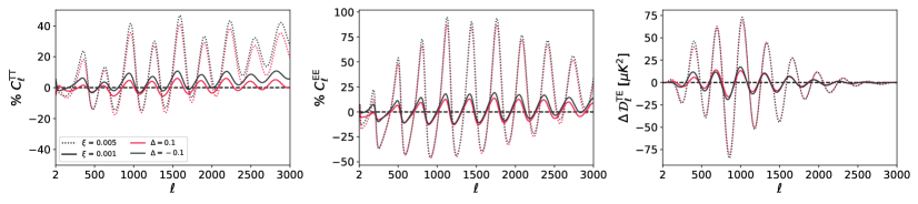
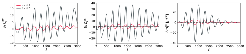
Figure 1: Differences with respect to the $\Lambda$CDM CMB lensed angular power spectra with IG (top panels) for $\xi=0.001,\,0.005$ (solid, dotted) and $\Delta=-0.1,\,0.1$ (black, red), and CC (bottom panels) for $\Delta=0.00001,\,0.0001$ (red, black). ${\cal D}_{\ell}\equiv\ell(\ell+1)C_{\ell}/(2\pi)$ are the band-power angular power spectra.

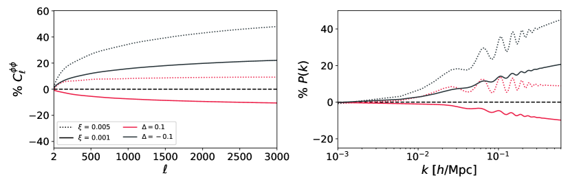
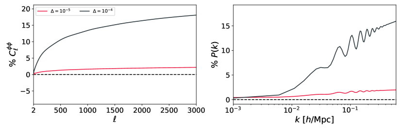
Figure 2: Relative differences of the CMB lensing potential angular power spectrum (left panels) and linear matter power spectrum at $z=0$ (right panels) for IG (top panels) with $\xi=0.001,\,0.005$ (solid, dotted) and $\Delta=-0.1,\,0.1$ (black, red), and CC (bottom panels) for $\Delta=0.00001,\,0.0001$ (red, black) with respect to the $\Lambda$CDM.

Fig. 2 shows that for $\Delta>0$ the CMB lensing potential spectrum $C_{\ell}^{\phi\phi}$ and the matter power spectrum at $z=0$ $P(k)$ can be smaller than in $\Lambda$CDM for small scales, a behavior which does not occur for $\Delta<0$ or for $\Delta=0$ [30]. In Fig. 3, we show the evolution of the background quantities $H(z)$, $\Omega_{\rm m}(z)$, $G_{\rm eff}/G(z)$, and $\sigma_{8}(z)$ for IG. We see that for $\xi=0.001$ and $\Delta=0.1$ the amplitude of matter perturbation today $\sigma_{8}$ is slightly smaller than the one in $\Lambda$CDM.

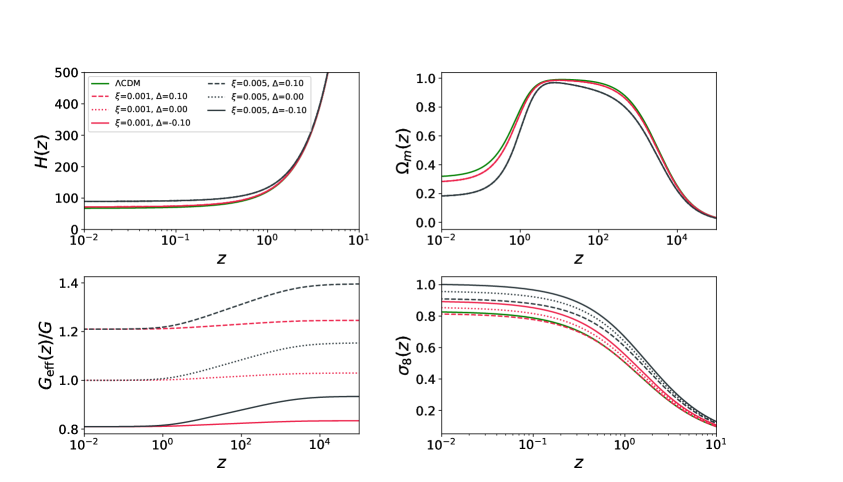
Figure 3: Evolution of $H(z)$ (top-left panel), $\Omega_{\rm m}=\rho_{\rm m}/(3H_{0}^{2})$ (top-right panel), $G_{\rm eff}(z)/G$ (bottom-left panel), and $\sigma_{8}(z)$ (bottom-right panel) as function of $z$ for $\xi=10^{-3},\ 5\times 10^{-3}$ and different choices of $\Delta$ from $\Delta=-0.1$ to $\Delta=0.1$.

2.2 A non-minimally coupled scalar field

We study $F(\sigma)=M_{\rm pl}^{2}+\xi\sigma^{2}$. In this case we find two different branches of the parameter space $\{\xi>0,\,\Delta<0\}$ (NMC+) and $\{\xi<0,\,\Delta>0\}$ (NMC$-$) in order to satisfy the positiveness of $\sigma$ and $F(\sigma)$ for all times, with

$$\left(\frac{\sigma_{0}}{M_{\rm pl}}\right)^{2}= \frac{1}{2(1+\Delta)^{2}\xi(1+6\xi)}\Bigg{[}-1+2\xi-2\Delta(2+\Delta)(1+3\xi)$$

$$+\sqrt{1+4\xi\left(-1+\xi+\Delta\left(2+\Delta\right)\left(-5+3\xi\left(-2+3\Delta\left(2+\Delta\right)\right)\right)\right)}\Bigg{]}\,.$$ (2.5)

The CC case $\xi=-1/6$ has to be treated separately

$$\left(\frac{\sigma_{0}}{M_{\rm pl}}\right)^{2}=18\frac{\left(1+\Delta\right)^{2}-1}{1+3\left(1+\Delta\right)^{2}}\,.$$ (2.6)

In the NMC case $\Delta$ can not be both negative and positive for the same branch of $\xi$ implying that for a given sign of $\xi$ the effective gravitational constant can be only larger or only smaller than the value of the gravitational constant. This is due to the assumption $N_{\rm pl}=M_{\rm pl}$ and the condition $F(\sigma)>0$ to avoid negative kinetic energy states in the tensor sector [55]. Fig. 5 shows that for $\Delta>0$ the CMB lensing potential spectrum $C_{\ell}^{\phi\phi}$ and the matter power spectrum at $z=0$ $P(k)$ can be smaller than in $\Lambda$CDM for small scales, a trend which does not occur for $\Delta<0$ or for $\Delta=0$ and $N_{\rm pl}\neq M_{\rm pl}$ [32].

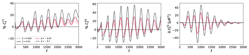
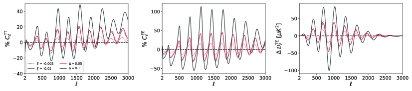
Figure 4: Differences with respect to the $\Lambda$CDM CMB lensed angular power spectra for NMC+ with $\xi=0.005,\,0.01$ (dotted, solid) and $\Delta=-0.05,\,-0.1$ (red, black), and for NMC- (bottom panels) with $\xi=-0.005,\,-0.01$ (dotted, solid) and $\Delta=0.05,\,0.1$ (red, black). ${\cal D}_{\ell}\equiv\ell(\ell+1)C_{\ell}/(2\pi)$ are the band-power angular power spectra.

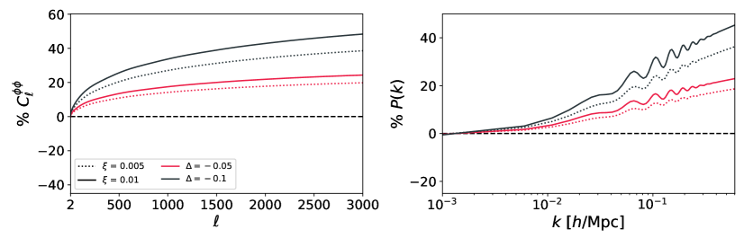
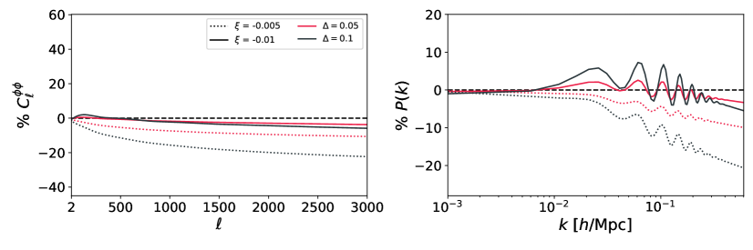
Figure 5: Relative differences of the CMB lensing potential angular power spectrum (left panels) and linear matter power spectrum at $z=0$ (right panels) for NMC+ (top panels) with $\xi=0.005,\,0.01$ (dotted, solid) and $\Delta=-0.05,\,-0.1$ (red, black), and for NMC- (bottom panels) with $\xi=-0.005,\,-0.01$ (dotted, solid) and $\Delta=0.05,\,0.1$ (red, black) with respect to the $\Lambda$CDM.

3 Methodology and datasets

In order to derive the constraints on the cosmological parameters we perform a Markov Chain Monte Carlo (MCMC) analysis by using the publicly available code MontePython [56, 57] connected to our modified version of the code CLASS [58, 59], i.e. CLASSig [30]. Mean values and uncertainties on the reported parameters, as well as the plotted contours, have been obtained using GetDist [60]. We use adiabatic initial conditions for the scalar field perturbations [29, 32].

We vary the six cosmological parameters for a flat $\Lambda$CDM concordance model, i.e. $\omega_{\rm b}$, $\omega_{\rm c}$, $H_{0}$, $\tau$, $\ln\left(10^{10}A_{\rm s}\right)$, $n_{\rm s}$, plus the extra parameters related to the coupling to the Ricci curvature. For IG $(N_{\rm pl}=0,\,\xi>0)$, we sample on the quantity $\zeta_{\rm IG}\equiv\ln\left(1+4\xi\right)$, according to [30, 31, 28] in the prior range $[0,\,0.039]$ and $\Delta\in[-0.3,\,0.3]$. For CC $(N_{\rm pl}=M_{\rm pl},\,\xi=-1/6)$, we sample on $\Delta\in[0,\,0.1]$. For NMC $(N_{\rm pl}=M_{\rm pl},\,\xi\neq 0)$, we sample separately on the positive branch with $\xi\in[0,0.3]$ and $\Delta\in[-0.1,\,0]$, and on the negative branch with $\xi\in[-0.3,0]$ and $\Delta\in[0,\,0.1]$. We assume 2 massless neutrino with $N_{\rm eff}=2.0328$, and a massive one with fixed minimum mass $m_{\nu}=0.06$ eV. We fix the primordial ^4He mass fraction $Y_{\rm p}$ according to the prediction from PArthENoPE [61, 62], by taking into account the relation with the baryon fraction $\omega_{\rm b}$ and the varying gravitational constant which enters in the Friedman equation during nucleosynthesis. We indeed consider the varying gravitational constant as an additional contribution to the effective relativistic species $\Delta N_{\rm eff}=\left[3.046+\frac{8}{7}\left(\frac{11}{4}\right)^{\frac{4}{3}}\right]\left(\frac{G_{\rm N}}{G}-1\right)$ in $Y_{\rm BBN}(\omega_{b},\,N_{\rm eff})$ at $z_{\rm BBN}$ [63].

We constrain the cosmological parameters using the CMB anisotropies measurements from the Planck 2018 legacy release (hereafter P18), in combination with BAO measurements from galaxy redshift surveys, and a Gaussian likelihood based on the determination of the Hubble constant from Hubble Space Telescope (HST) observations (hereafter R19), i.e. $H_{0}=(73.4\pm 1.4)$ km s^-1Mpc^-1 [64]. Our CMB measurements combine temperature, polarization, and weak lensing CMB anisotropies angular power spectra [65, 66]. The high-multipoles likelihood is based on Plik likelihood, the low-$\ell$ likelihood is based on the Commander likelihood (temperature-only) plus the SimAll EE-only likelihood, the CMB lensing likelihood is considered on the conservative multipoles range, i.e. $8\leq\ell\leq 400$. We marginalize over foreground and calibration nuisance parameters of the Planck likelihoods which are also varied together with the cosmological ones. We use BAO data from Baryon Spectroscopic Survey (BOSS) DR12 [67] consensus results in three redshift slices with effective redshifts $z_{\rm eff}=0.38,\,0.51,\,0.61$ in combination with measure from 6dF [68] at $z_{\rm eff}=0.106$ and the one from SDSS DR7 [69] at $z_{\rm eff}=0.15$. In some of our analysis, we also include a Gaussian prior on $S_{8}\equiv\sigma_{8}\sqrt{\Omega_{\rm m}/0.3}$, $p(S_{8})$, based on the inverse-variance weighted combination of the weak lensing measurements of DES [70], KV-450 [71, 72], and HSC [73], i.e. $S_{8}=0.770\pm 0.017$.

4 Results

In this section we present the results for IG, CC, and NMC based on the combination of Planck 2018 data (P18) [65, 66], BOSS DR12 BAO consensus data [67], and a Gaussian prior on $H_{0}$ from [64]. We collect tables with the full constraints on the cosmological parameters obtained with our MCMC analysis in App. A and the full triangle plots with the standard cosmological parameters in App. B.

For IG, we obtain the following joint constraints at 68% CL correspond to $\Delta=-0.032^{+0.029}_{-0.025}$, $10^{3}\,\xi<2.1$ (P18), $\Delta=-0.022\pm 0.023$, $10^{3}\,\xi<0.82$ (P18 + BAO), and $\Delta=-0.026\pm 0.024$, $10^{3}\,\xi=0.74^{+0.52}_{-0.54}$ (P18 + BAO + R19). Constraints on the ratio of the effective gravitational constant correspond to $G_{\rm eff}/G=0.938^{+0.056}_{-0.049}$ (P18), $G_{\rm eff}/G=0.957\pm 0.045$ (P18 + BAO), and $G_{\rm eff}/G=0.949\pm 0.048$ (P18 + BAO + R19) at 68% CL.

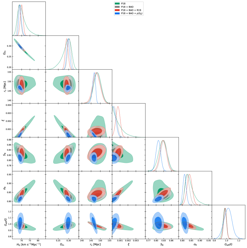
Figure 6: Marginalized joint 68% and 95% CL regions 2D parameter space using the $Planck$ legacy data (green), its combination with BAO DR12, i.e. P18 + BAO (gray), and P18 + BAO + R19 (red), for the IG model. The blue contours include a Gaussian prior on $S_{8}$.

In Fig. 7, we compare the results with the case $\Delta=0$ over the parameter space $H_{0}$-$\xi$. We see that relaxing the condition on $G_{\rm eff}$, i.e. Eq. (2.3), the constraints on the coupling become larger: $10^{3}\,\xi<2.1,\,<0.82,\,=0.74^{+0.52}_{-0.54}$ at 95% CL with $\Delta\neq 0$ compared to $10^{3}\,\xi<0.96,\,<0.68,\,=0.62^{+0.48}_{-0.46}$ with $\Delta=0$ for P18, P18 + BAO, P18 + BAO + R19 respectively. In particular, varying $\Delta$ the uncertainties on $\xi$ become two times larger using CMB data alone, $\sim 21\%$ larger for P18 + BAO, and $\sim 13\%$ larger for P18 + BAO+ R19. Once we include R19, the larger value of $H_{0}$ comes with a $2.5\sigma$ detection of the coupling $\xi=0.00074^{+0.00052}_{-0.00054}$ at 95% CL.

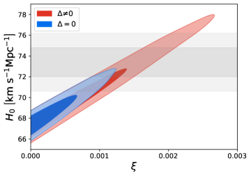
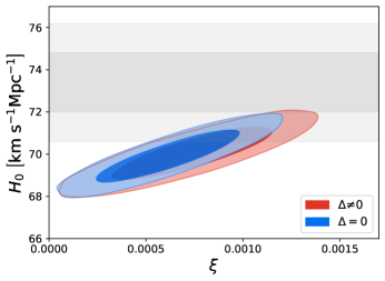
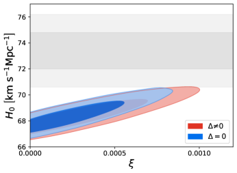
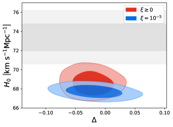
Figure 7: Marginalized joint 68% and 95% CL regions 2D parameter space using the $Planck$ legacy data (upper left panel), its combination with BAO DR12, i.e. P18 + BAO (bottom left panel), and P18 + BAO + R19 (upper right panel) for the IG model with $\Delta\neq 0$ ($\Delta=0$) in red (blue). We show also the combination P18 + BAO on the parameter space $H_{0}$-$\Delta$ where we fix $\xi=10^{-5}$ (bottom right panel).

The CC case remains tightly constrained, as shown in Fig. 8, see also Refs. [32, 28, 49]. The large value of $\xi=-1/6$ requires a small value of the scalar field $\sigma(z)/M_{\rm pl}$ at early time in order to satisfy the CMB constraints on $F(\sigma)$. This is reflected on a tight constraint $\Delta<2.3\times 10^{-5}$ at 95% CL for P18 + BAO (analogously to the constraints $N_{\rm pl}<1.000023\$M_pl [28] at 95% CL for P18 + BAO). We show in Fig. 9 how negligible is the dependence on different priors for the CC case either sampling linearly on $\Delta$ with $N_{\rm pl}=M_{\rm pl}$ as done here or on $N_{\rm pl}>M_{\rm pl}$ as in Refs. [32, 28], the posterior probability for cosmological parameters are the same.

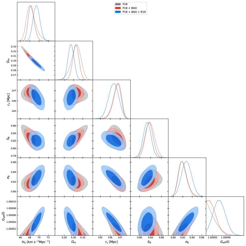
Figure 8: Marginalized joint 68% and 95% CL regions 2D parameter space using the $Planck$ legacy data (gray), its combination with BAO DR12, i.e. P18 + BAO (red), and P18 + BAO + R19 (blue) for the CC model.

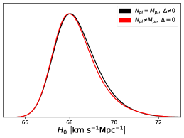
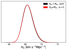
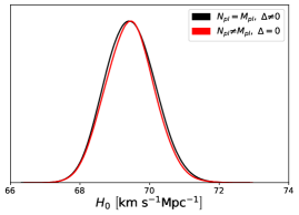
Figure 9: Marginalized joint 68% and 95% CL regions 2D parameter space using the $Planck$ legacy data (left panel) in combination with BAO DR12, i.e. P18 + BAO (central panel), and P18 + BAO + R19 (right panel) for the CC model with $\Delta\neq 0$ ($\Delta=0$) in red (black).

For NMC+ (NMC$-$) we sample $\Delta$ over range $[-0.1,\,0]$ ($[0,\,0.1]$) so that the value of the effective gravitational constant today is always smaller (larger) than $G$. Constraints on $\Delta$ for NMC+ correspond to $\Delta>-0.018$ (P18 + BAO) at 95% CL and to $\Delta=-0.0072^{+0.0053}_{-0.0020}$ (P18 + BAO + R19) at 68% CL. Constraints on the ratio of the effective gravitational constant correspond to $G_{\rm eff}/G>0.964$ (P18 + BAO) at 95% CL and $G_{\rm eff}/G=0.986^{+0.011}_{-0.0041}$ (P18 + BAO + R19) at 68% CL. Analogously for NMC$-$, we obtain $\Delta<0.021$ (P18 + BAO) and $\Delta<0.030$ (P18 + BAO + R19) both at 95% CL. Constraints at 95% CL on the ratio of the effective gravitational constant correspond to $G_{\rm eff}/G<1.04$ (P18 + BAO) and $G_{\rm eff}/G<1.06$ (P18 + BAO + R19).

As previously observed in Refs. [32, 28, 48], there is a strong degeneracy between the coupling parameters for the form $F(\sigma)=N_{\rm pl}^{2}+\xi\sigma^{2}$ also in this case with $N_{\rm pl}=M_{\rm pl}$ opening to $\Delta\neq 0$. Since our data constrains the deviations ${\cal O}(\xi\sigma^{2}/M_{\rm pl}^{2})$ from $M_{\rm pl}^{2}$, we loose constraining power on $\xi$ for small values of $\Delta$ corresponding to the limit for $\sigma_{0}\to 0$ (see Eq. (2.2)).

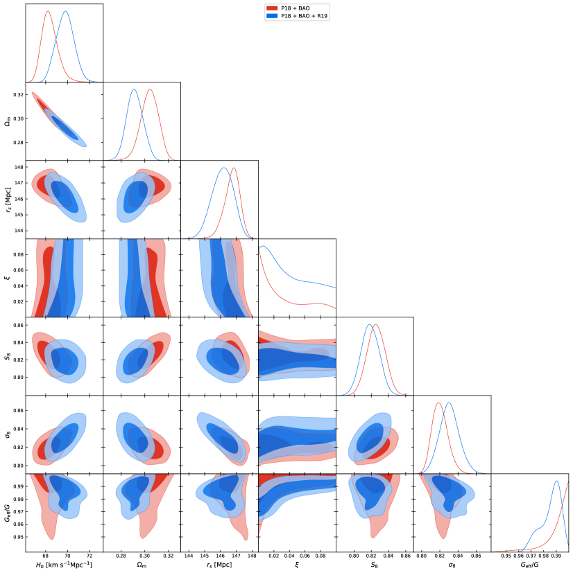
Figure 10: Marginalized joint 68% and 95% CL regions 2D parameter space using the $Planck$ legacy data in combination with BAO DR12, i.e. P18 + BAO (red) and P18 + BAO + R19 (blue) for the NMC+ model.

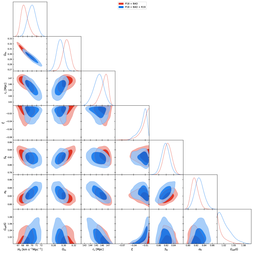
Figure 11: Marginalized joint 68% and 95% CL regions 2D parameter space using the $Planck$ legacy data in combination with BAO DR12, i.e. P18 + BAO (red) and P18 + BAO + R19 (blue) for the NMC- model.

4.1 Implications for the $H_{0}$ and $S_{8}$ tensions

As already pointed out in previous studies (see Refs. [30, 28]), these models alleviate the $H_{0}$ tension compared to the $\Lambda$CDM concordance model thanks to the early-time contribution to the radiation density budget in the radiation-dominated epoch and to the modification of the background expansion history. Extending the models to $\Delta\neq 0$, we find that the constraints on $H_{0}$ from CMB alone are larger while they are slightly affected once BAO are included, see Figs. 7-9. We find for IG $H_{0}=\left(70.2^{+1.2}_{-3.1}\right)$, $\left(68.61^{+0.72}_{-0.94}\right)$, $\left(70.04\pm 0.83\right)$ km s^-1 Mpc^-1 with $\Delta\neq 0$ at 68% CL, compared to $H_{0}=\left(68.82^{+0.8}_{-1.7}\right)$, $\left(68.57^{+0.62}_{-0.90}\right)$, $\left(69.93\pm 0.81\right)$ km s^-1 Mpc^-1 with $\Delta=0$ for P18, P18 + BAO, P18 + BAO + R19 respectively. Indeed, the larger value of $H_{0}$ inferred is mainly driven by $\xi$ once BAO are included. In Fig. 7 (bottom-right panel), we show that the marginalized posterior distribution of $H_{0}$ shrinks towards smaller values when fixing $\xi=10^{-5}$. The differences are smaller for the CC model.

NMC scalar-tensor models usually lead to a larger value of $\sigma_{8}$, in particular a positive correlation between the NMC parameters and both $H_{0}$ and $\sigma_{8}$ alleviating the $H_{0}$ tension while exacerbating the discrepancy between the value of $S_{8}$ inferred and the one observed by galaxy shear experiments. These theories predict a decreasing effective gravitational constant which is always larger than the Newton’s measured constant if we impose Eq. (2.3) [30, 32]. Relaxing the boundary condition on the present value of the effective gravitational constant, it is possible to generate a regime of weaker or stronger gravity at low redshift connected with an higher or lower value of $\sigma_{8}$ compared to the $\Lambda$CDM prediction; in particular it is possible to reduce the value of $\sigma_{8}$ for values $\Delta>0$ in IG and NMC$-$ keeping a larger value of $H_{0}$, as shown in Figs. 2-5 and in Figs. 6-8-10-11, in contrast to what happens in NMC with $\Delta=0$ or in EDE models.

Finally we compare the theoretical predictions of different models on the parameters $S_{8}$ and $H_{0}$ for the combination of CMB and BAO data, see Fig. 12. As it can be seen for IG in Fig. 3, while $\xi$ affects all the quantities plotted and can be connected to both the $H_{0}$ and $S_{8}$ tension, $\Delta$ plays a role mainly for the $S_{8}$ tension and does not affect significantly the value of the Hubble constant, see also Ref. [51]. In order to put to test a possible connection between $\Delta$ and $S_{8}$, we test the addition of a Gaussian prior $p(S_{8})$ on $S_{8}$ to our fit. In this way for IG we obtain an higher value for $\Delta=0.001^{+0.035}_{-0.029}$ at 68% CL and approximately a 2$\sigma$ decrease in the value of $S_{8}$, compared to P18 + BAO results in Table 2. We leave the purpose of a full weak lensing analysis to a future work.

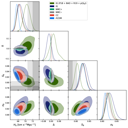
Figure 12: Marginalized joint 68% and 95% CL regions 2D parameter space using the $Planck$ legacy data in combination with DR12 BAO data (P18 + BAO) for all the models analysed (if not otherwise stated). The gray bands denote the local Hubble parameter measurement from R19, i.e. $H_{0}=(73.4\pm 1.4)$ km s^-1Mpc^-1 [64], and the inverse-variance weighted combination of the DES/KV-450/HSC weak lensing measurements, i.e. $S_{8}=0.770\pm 0.017$ [70, 71, 72, 73].

5 Forecasts

We perform the Fisher forecast analysis for the 6 standard cosmological parameters $\omega_{c}$, $\omega_{b}$, $H_{0}$, $\tau$, $n_{s}$, $\ln(10^{10}A_{s})$, and the extra parameters $\xi$, $\Delta$. For the CMB we consider also the optical depth at reionization $\tau$ and then we marginalize over it before combining it with the CMB Fisher matrix with the LSS ones. For the standard parameters, we assume as fiducial model a flat cosmology with best-fit parameters corresponding to $\omega_{\rm c}=0.12$, $\omega_{\rm b}=0.02237$, $H_{0}=67.36$ km s^-1 Mpc^-1, $\tau=0.0544$, $n_{\rm s}=0.9649$, $\ln\left(10^{10}\ A_{\rm s}\right)=3.044$, and one massive neutrino with $m_{\nu}=0.06$ eV consistent with the results of $Planck$ DR3 [18]. As fiducial value for the extra parameters for IG, we choose $\xi=10^{-5}$ and $\Delta=10^{-3}$.

5.1 Cosmic microwave background anisotropies

As specifications for future CMB measurements, we consider the combination of the Lite (Light) satellite for the study of B-mode polarization and Inflation from cosmic background Radiation Detection (LiteBIRD) [74], selected by the Japan Aerospace Exploration Agency (JAXA) as a strategic large class mission, and CMB-S4 [75] as representative of current and future CMB experiments from ground, which also include SPT-3G [76], Simons Observatory [77]. For LiteBIRD, we consider the multipole range between $2\leq\ell<30$. For CMB-S4, following [78, 75], we assume a sensitivity $\sigma_{\rm T}^{1/2}=\sigma_{\rm P}^{1/2}/\sqrt{2}=1\ \mu$K-arcmin with a beam resolution of $\theta_{\rm FWHM}=3$ arcmin over 40% of the sky, with $\ell_{\rm min}=30$ and a different cut at small scales of $\ell^{\rm T}_{\rm max}=3000$ in temperature and $\ell^{\rm P}_{\rm max}=5000$ in polarization motivated by the excess of foreground contamination expected on the small scales in temperature. We use the CMB lensing information in the range $30\leq\ell\leq 3000$, assuming the minimum variance quadratic estimator for the lensing reconstruction, combining the TT, EE, BB, TE, TB, and EB estimators, calculated according to Ref. [79] and applying iterative lensing reconstruction (see Ref. [80, 81]).

5.2 Spectroscopic galaxy clustering

To describe the main galaxy clustering observable, we follow [78] and we modify the observed galaxy power spectrum in order to account for the non-linear effects according to [82, 83, 84, 85]. The full anisotropic non-linear observed galaxy power spectrum is given by

$$P_{\text{obs}}(k,\mu;\,z) = \frac{D^{2}_{{\rm A},r}(z)H(z)}{D^{2}_{\rm A}(z)H_{r}(z)}\left\{\frac{\left[b\sigma_{8}(z)+f\sigma_{8}(k,z)\mu^{2}\right]^{2}}{1+k^{2}\mu^{2}f^{2}(k,z)\sigma_{\rm p}^{2}(z)}\right\}\times$$ (5.1)

$$\times \frac{P_{\text{dw}}(k,\mu;z)}{\sigma^{2}_{8}(z)}F_{z}(k,\mu;z)+P_{\text{s}}(z)\,,$$

where the subscript $r$ refers to the reference (or fiducial) cosmology. $P_{\rm s}(z)$ is a scale-independent nuisance parameter due to imperfect removal of shot-noise. The Alcock-Paczynski (AP) effect takes into account the incorrect cosmological models from the fiducial one and it is parameterised through the rescaling of the angular diameter distance $D_{\rm A}(z)$ and the Hubble parameter $H(z)$. The AP effect enters as a multiplicative factor to the galaxy power spectrum, and in both $k$ and $\mu$, see [86, 85] for more details. The term in the curly brackets in Eq. (5.1) is the redshift space distortion (RSD) [87] which is corrected for the non-linear finger-of-God (FoG) effect. The RSD is parameterised through the galaxy bias $b(z)$ and the growth rate $f(k,z)$, both multiplied by the root mean square of matter density fluctuation $\sigma_{8}(z)$, whereas $\mu$ is the cosine of the angle of the wave mode with respect to the line of sight pointing into the direction $\hat{r}$, and $k$ is the scale of the perturbation.

$P_{\rm dw}(k,\mu;\,z)$ is the de-wiggled power spectrum which models the smearing of the BAO signal due to non-linearities, and it is defined as

$$P_{\text{dw}}(k,\mu;z)=P_{\rm m}(k;z)\,\text{e}^{-g_{\mu}k^{2}}+P_{\text{nw}}(k;z)\left(1-\text{e}^{-g_{\mu}k^{2}}\right)\,,$$ (5.2)

where $P_{\rm nw}(k;z)$ is the ‘no-wiggle’ power spectrum obtained directly from the matter power spectrum but without BAO features. Modified gravity models usually predict a scale dependent growth rate $f(z,k)$ which needs to be taken into account when evaluating the Fisher matrix. For the model used in this work, we found that the deviation from a constant value is at most $0.1\%$ over the whole range of $k$ used in the analysis. Hence, we can safely assume the growth rate to be independent of scale in the non-linear terms appearing in $P_{\rm dw}$. The pairwise velocity dispersion, $\sigma_{\rm p}(z)$ and the velocity dispersion, $\sigma_{\rm v}(z)$ are then equal and the function $g_{\mu}$ in Eq. (5.2)

$$\sigma^{2}_{\rm v}(z)=\sigma^{2}_{\rm p}(z) = \frac{1}{6\pi^{2}}\int{\rm d}k\,P_{\rm m}(k,z)\,,$$ (5.3)

$$g_{\mu}(z,\mu) \simeq \sigma^{2}_{\rm v}(z)\left[1-\mu^{2}+\mu^{2}\left[1+f(\bar{k},z)\right]^{2}\right]\,.$$ (5.4)

where we choose the mean value of the $\bar{k}=0.05\,h/{\rm Mpc}$. Finally, the total galaxy power spectrum in Eq. (5.1) includes the errors on redshift through the factor

$$F_{z}(k,\mu;z)=\text{e}^{-k^{2}\mu^{2}\sigma_{r}^{2}(z)}\,,$$ (5.5)

where $\sigma_{r}^{2}(z)=c(1+z)\sigma_{0,z}/H(z)$ and $\sigma_{0,z}$ is the error on the measured redshifts.

The no-wiggle matter power spectrum $P_{\rm nw}(k;z)$ entering Eq. (5.2) has been obtained using a Savitzky-Golay filter to the matter power spectrum $P_{\rm m}(k;z)$. The Savitzky-Golay filter is usually applied to noisy data in order to smooth their behavior. In practice, we treat the BAO wiggles in the matter power spectrum as if they were noise in the overall shape of the matter power spectrum; by smoothing the noise, we recover exactly the same shape and amplitude of the matter power spectrum without the BAO wiggles, see [88].

The final Fisher matrix for the galaxy clustering observable for one redshift bin $z_{i}$ is

$$F_{\alpha\beta}(z_{i})=\frac{1}{8\pi^{2}}\int_{-1}^{1}{\rm d}\mu\int_{k_{\rm min}}^{k_{\rm max}}V_{\rm eff}(z_{i},k)\cdot\frac{\partial\ln P_{\rm obs}(k,\mu;\,z_{i})}{\partial p_{\alpha}}\frac{\partial\ln P_{\rm obs}(k,\mu;\,z_{i})}{\partial p_{\beta}}\cdot k^{2}{\rm d}k$$ (5.6)

where the derivatives are evaluated at the parameter values of the fiducial model and $V_{\rm eff}$ is the effetive volume of the survey, given by

$$V_{\rm eff}(k,\mu;\,z)=V_{\rm s}\left[\frac{n(z)P_{\rm obs}(k,\mu;\,z)}{1+n(z)P_{\rm obs}(k,\mu;\,z)}\right]^{2}$$ (5.7)

being $V_{\rm s}$ the volume of the survey and $n(z)$ the number of galaxies in a redshift bin.

In our analysis we used 8 cosmological parameters constant for all redshifts and 2 redsfhit dependent parameters

$$p_{\alpha}=\left\{\Omega_{\rm m},\,\Omega_{\rm b},\,h,\,n_{\rm s},\,\xi,\,\Delta,\,\sigma_{8},\,\ln b\sigma_{8}(z),\,P_{\rm s}(z)\right\}$$ (5.8)

where $\Omega_{X}$ corresponds to the density parameter at current time and $\sigma_{8}\equiv\sigma_{8}(z=0)$. The total Fisher matrix for GC is constructed summing up directly the elements of the Fisher matrices at each bin for the redsfhit independent parameters, whereas the z-dependent parameters will be added in sequence to the final Fisher matrix. In the specific, the final Fisher matrix has dimensions $7+n_{\rm bin}\times 2$, where $n_{\rm bin}$ is the number of redshift bins. Both $\ln b\sigma_{8}(z)$ and $P_{\rm s}(z)$ are nuisance parameters and they are marginalized over.

We present GC results for three different range of wavenumbers: quasi-linear scales with $k_{\rm max}^{\rm GC}=0.15\ h/$Mpc and two case including non-linear scales with $k_{\rm max}^{\rm GC}=0.25,\,0.30\ h/$Mpc.

We forecast the GC constraints for the ground-based Dark Energy Spectroscopic Instrument (DESI) [89]. Following [90], we consider a unified effective sample combining the populations of LRGs, ELGs and QSOs, covering thirteen redshift bins between z = 0.6 and 1.9 with width of $\Delta z=0.1$, with a volume of the survey of $14,000\,{\rm deg}^{2}$. Finally, we complete the analysis by include low-redshift spectroscopic information from BOSS [91], the volume of the survey is $9,329\,{\rm deg}^{2}$, in a redshift range $z\in[0.2,\,0.75]$ divided in two bins with $\Delta z=[0.3,\,0.25]$.

5.3 Weak gravitational lensing

Here we report the main equations of the weak lensing tomographic signal and we refer to the literature for further details [85, 92, 93, 94]. The weak lensing convergence power spectrum is a linear function of the matter power spectrum convoluted with the lensing properties of the survey. In the $\Lambda$CDM cosmology, we can write it as

$$P_{i\,j}(\ell)=H^{4}_{0}\int_{0}^{\infty}\frac{{\rm d}z}{H^{2}(z)}W_{i}(z)W_{j}(z)P_{\rm nl}\left(k=\frac{\ell\,H_{0}}{r(z)}\,,z\right)\,,$$ (5.9)

where $\ell$ is the multipole number, $r(z)$ is the comoving distance between lens and objects, $H(z)$ is the Hubble parameter, and the subscripts $i\,,j$ refer to the redshift bins around the redshifts $z_{i}$ and $z_{j}$. The window function, $W_{i}(z)$, which takes into account the lensing properties of space, is defined as

$$W_{i}(z)=\frac{3}{2}\left(\frac{H_{0}}{c}\right)^{2}\Omega_{m}(1+z)r(z)\int_{z}^{z_{\rm max}}{\rm d}z^{\prime}D(x)\left[1-\frac{r(z)}{r(z^{\prime})}\right]$$ (5.10)

being $z_{\rm max}$ the maximum redshift of the $i$-th bin and the radial distribution function of galaxies is

$$D(z)=z^{\alpha}\exp\left[-\left(z/z_{0}\right)^{\beta}\right]$$ (5.11)

where $\alpha\,,\beta\,,z_{0}$ are constants that depend on the survey strategy. For the Vera C. Rubin Observatory’s Legacy Survey of Space and Time (LSST), we assume $\alpha=1.27$, $\beta=1.02$ and $z_{0}=0.5$ [95, 96]. Moreover, we consider a survey up to $z_{\rm max}=3$ divided into 10 bins each containing the same number of galaxies.

The Fisher matrix for the weak lensing signal is

$$F_{\alpha\beta}=f_{\rm sky}\sum_{\ell}\frac{(2\ell+1)\Delta\ell}{2}\frac{\partial P_{ij}}{\partial p_{\alpha}}C^{-1}_{jk}\frac{\partial P^{-1}_{km}}{\partial p_{\beta}}C^{-1}_{mi}$$ (5.12)

where $\Delta\ell$ is the step in multipoles, to which we chose 100 step in logarithm scale, and $f_{\rm sky}=0.4363$; whereas $p_{\alpha}$ are the cosmological parameters. The covariances are defined as

$$C_{jk}=P_{jk}+\delta_{jk}\langle\gamma^{2}_{\rm int}\rangle n^{-1}_{j}$$ (5.13)

where $\gamma_{\rm int}$ is the rms intrinsic shear, which we assume $\langle\gamma^{2}_{\rm int}\rangle=0.26$.

The number of galaxies per steradians in each bin is defined as:

$$n_{j}=3600d\left(\frac{180}{\pi}\right)^{2}\hat{n}_{j}$$ (5.14)

where the number density is $d=26$ galaxy per arcmin and $\hat{n}_{j}$ is the fraction of sources that belongs to the $j$-th bin.

The final set of parameter for WL is

$$p_{\alpha}=\left\{\Omega_{\rm m},\,\Omega_{\rm b},\,h,\,n_{\rm s},\,\xi,\,\Delta,\,\sigma_{8}\right\}\,.$$ (5.15)

We present WL results for two different range of multipoles: a conservative case with $\ell_{\rm max}^{\rm WL}=1500$ and a case including all the information down to $\ell_{\rm max}^{\rm WL}=5000$.

We study the non-linear evolution of the matter power spectrum $P_{\rm nl}(k,z)$ with a modified version of the COmoving Lagrangian Accelerator (COLA) code [97, 98]. We generate simulations with $N=1024^{3}$ particles in a box size $L=1024\ {\rm Mpc}/h$ to cover large scales and $N=512^{3}$ particles in a box size $L=200\ {\rm Mpc}/h$ to cover the small scales, for the fiducial parameters used in the forecast analysis and $\xi=0.0001,0.001,0.01$. The variation of $\Delta$ is propagated through the linear matter power spectrum [51]. Fig. 13 shows the relative differences to $\Lambda$CDM.

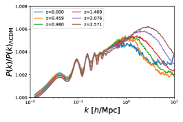
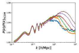
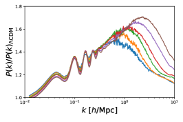
Figure 13: Relative difference of the matter power spectrum with respect to $\Lambda$CDM from the simulations of IG for $\xi=0.0001,0.001,0.01$ from left to right.

5.4 Results

We carry out a Fisher matrix analysis using $\xi$ and $\Delta$ in addition to the standard $\Lambda$CDM cosmological parameters. We marginalize the CMB Fisher matrix over the optical depth parameter $\tau$ and we project it over the LSS parameters in Eq. (5.15). Uncertainties on the cosmological parameters are calculated as the square root of the diagonal elements of the inverse of the Fisher matrix $\sqrt{\left(F^{-1}\right)_{\alpha\alpha}}$.

	$10^{3}\sigma(\xi)$	$10^{2}\sigma(\Delta)$
S4+LiteBIRD	0.14	0.7
BOSS+DESI ($k_{\rm max}^{\rm GC}=0.15,\,0.25,\,0.30$ $h/$Mpc)	1.6/0.86/0.76	18/11/9.9
LSST ($\ell_{\rm max}^{\rm WL}=1500/5000$)	2.1/1.2	8.9/5.4
S4+LiteBIRD	0.061/0.04/0.035	0.62/0.61/0.61
+ BOSS+DESI ($k_{\rm max}^{\rm GC}=0.15,\,0.25,\,0.30$ $h/$Mpc)
S4+LiteBIRD	0.031/0.020	0.54/0.44
+ LSST ($\ell_{\rm max}^{\rm WL}=1500/5000$)
BOSS+DESI ($k_{\rm max}^{\rm GC}=0.15,\,0.25,\,0.30$ $h/$Mpc)	0.49/0.43/0.40	7.0/6.6/6.2
+ LSST ($\ell_{\rm max}^{\rm WL}=1500$)
BOSS+DESI ($k_{\rm max}^{\rm GC}=0.15,\,0.25,\,0.30$ $h/$Mpc)	0.43/0.34/0.33	4.1/3.7/3.5
+ LSST ($\ell_{\rm max}^{\rm WL}=5000$)
S4+LiteBIRD	0.029/0.024/0.023	0.51/0.49/0.49
+ BOSS+DESI ($k_{\rm max}^{\rm GC}=0.15,\,0.25,\,0.30$ $h/$Mpc)
+ LSST ($\ell_{\rm max}^{\rm WL}=1500$)
S4+LiteBIRD	0.019/0.018/0.017	0.43/0.41/0.41
+ BOSS+DESI ($k_{\rm max}^{\rm GC}=0.15,\,0.25,\,0.30$ $h/$Mpc)
+ LSST ($\ell_{\rm max}^{\rm WL}=5000$)

Table 1: Marginalized uncertainties (68% CL) for $\xi=10^{-5}$ and $\Delta=10^{-3}$.

We collect the uncertainties for the single probes and the various combinations of those in Tab. 1. The uncertainties from single surveys are dominated by the CMB information. By the expected future measurements of CMB anisotropies from the combination of LiteBIRD and CMB-S4, which constrain both distance measurements as well as the growth rate at early times, we obtain 68% CL uncertainties $10^{4}\,\sigma(\xi)\simeq 1.4$ and $10^{2}\,\sigma(\Delta)\simeq 0.7$. These results improve the current Planck constraints by an order of magnitude on $\xi$ and by a factor of 4 on $\Delta$. Uncertainties on the coupling $\xi$ are consistent with the results obtained in Ref. [78] for IG with $\Delta=0$ showing no appreciable widening of the constraints for such future experiments.

In Fig. 14, we can see the important role that the complementarity between early-time and late-time cosmological probes plays. It is well established [99, 78] that the CMB and late-time measurements will combine to supply powerful constraints mitigating the degeneracies between $H_{0}$ and the coupling $\xi$ parameters. While GC data alone constrain better the coupling $\xi$, WL measurements are more sensitive to $\Delta$.

Finally, we derive tighter constraints from the combination of our three cosmological probes, which are $10^{5}\,\sigma(\xi)\simeq 1.7$ and $10^{3}\,\sigma(\Delta)\simeq 4.1$ for $k_{\rm max}^{\rm GC}=0.30\ h/$Mpc and $\ell_{\rm max}^{\rm WL}=5000$. It is interesting to note that these constraints are weakly affected ($<5\%$) by reducing the GC nonlinear information to $k_{\rm max}^{\rm GC}=0.15\ h/$Mpc.

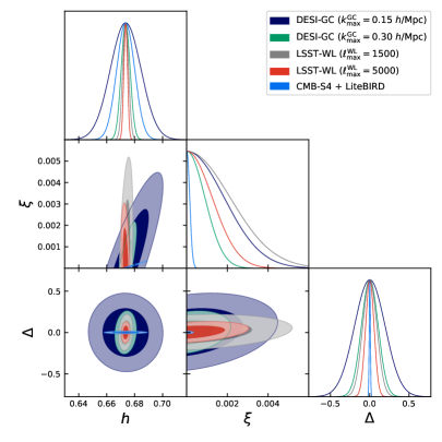
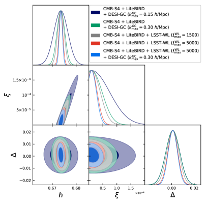
Figure 14: Left: marginalized 68% and 95% CL constraints on the parameter space $h$-$\xi$-$\Delta$ from single probes alone. Right: marginalized 68% and 95% CL constraints on the parameter space $h$-$\xi$-$\Delta$ from different combination of probes.

6 Conclusions

We have studied general constraints on the gravitational constant from cosmology. We have used the framework of a scalar field non-minimally coupled to the Ricci scalar, i.e. the simplest scalar-tensor theory of gravity, to study self-consistently variations in time and space of the gravitational constant. Going beyond what previously done, in this paper we have investigated in a direct way the effect of an imbalance $\Delta$ between the effective gravitational constant and G, i.e. $G_{\rm eff}(z=0)=G(1+\Delta)^{2}$.

We computed the effects of the imbalance $\Delta$ on cosmological observables and computed how current cosmological data can constrain it by also allowing the coupling to the Ricci scalar and the rest of cosmology to vary. Planck 2018 data in combination with BAO from BOSS DR12 data constrain the imbalance to $\Delta=-0.022\pm 0.023$ at 68% CL and the coupling parameter to $10^{3}\,\xi<0.82$ at 95% CL for $F(\sigma)=\xi\sigma^{2}$ and for a non-minimally coupled scalar field with $F(\sigma)=M^{2}_{\rm pl}+\xi\sigma^{2}$ constrain the imbalance to $\Delta>-0.018$ ($<0.021$) and the coupling parameter to $\xi<0.089$ ($\xi>-0.041$) both at 95% CL. These bounds correspond to constrain $G_{\rm eff}(z=0)/G$ to about 4-15% at 95% CL. By allowing $\Delta$ to vary the constraints on the coupling to the Ricci scalar $\xi$ degrade with respect to $\Delta=0$ [28].

We also explored the limit that could be achieved by future experiments. We forecasted $\sigma(G_{\rm eff}(z=0)/G)\simeq 0.014$ at 68% CL by the combination of CMB anisotropy measurements from LiteBIRD and CMB-S4. Combining the CMB information with galaxy clustering from BOSS + DESI and galaxy shear from LSST we found $\sigma(G_{\rm eff}(z=0)/G)\simeq 0.008$ at 68% CL.

We note that the extended phenomenology studied here is not only relevant for testing gravity on large scales, but can also help in interpreting the current tensions in the estimates of cosmological parameters from different observations. Since the first Planck data release, we noticed how one of the simplest scalar-tensor gravity model such as induced gravity (equivalent to Jordan-Brans-Dicke) with a quartic potential could accommodate for a larger value of $H_{0}$ compared the one in $\Lambda$CDM [30] due to a degeneracy between the coupling to the Ricci scalar and $H_{0}$. Subsequent studies generalized this result for different simple potentials and couplings [31, 32, 28]. While this model is able to accommodate for a smaller values of $\sigma_{8}$ for large value of $\Delta>0$, we do not see any reduction in term of the parameter $S_{8}$ by fitting Planck 2018 CMB data and BOSS DR12 measurements. Work in this direction is in progress.

Appendix A Tables

	P18	P18 + BAO	P18 + BAO + R19
$\omega_{\rm b}$	$0.02218\pm 0.00024$	$0.02221\pm 0.00024$	$0.02223\pm 0.00025$
$\omega_{\rm c}$	$0.1198\pm 0.0013$	$0.1200\pm 0.0011$	$0.1201\pm 0.0011$
$H_{0}$ [km s-1Mpc-1]	$70.2^{+1.2}_{-3.1}$	$68.61^{+0.72}_{-0.94}$	$70.04\pm 0.83$
$\tau$	$0.0551\pm 0.0075$	$0.0543\pm 0.0072$	$0.0555^{+0.0067}_{-0.0079}$
$\ln\left(10^{10}A_{\rm s}\right)$	$3.041\pm 0.017$	$3.040\pm 0.016$	$3.043\pm 0.017$
$n_{\rm s}$	$0.9608\pm 0.0077$	$0.9604\pm 0.0074$	$0.9617\pm 0.0077$
$\zeta_{\rm IG}$	$<0.0084$ (95% CL)	$<0.0033$ (95% CL)	$0.0029\pm 0.0011$
$\Delta$	$-0.032^{+0.029}_{-0.025}$	$-0.022\pm 0.023$	$-0.026\pm 0.024$
$\xi$	$<0.0021$ (95% CL)	$<0.00082$ (95% CL)	$0.00074^{+0.00052}_{-0.00054}$ (95% CL)
$\gamma_{\rm PN}$	$>0.9917$ (95% CL)	$>0.9968$ (95% CL)	$0.9971\pm 0.0011$
$\delta G_{\mathrm{N}}/G_{\mathrm{N}}$ (z=0)	$>-0.060$ (95% CL)	$>-0.0240$ (95% CL)	$-0.0216\pm 0.0079$
$10^{13}\dot{G}_{\mathrm{N}}/G_{\rm N}$ (z=0) [yr-1]	$>-2.34$ (95% CL)	$>-0.98$ (95% CL)	$-0.88\pm 0.32$
$G_{\mathrm{N}}/G$ (z=0)	$0.937^{+0.057}_{-0.050}$	$0.956\pm 0.045$	$0.948\pm 0.048$
$G_{\mathrm{eff}}/G$ (z=0)	$0.938^{+0.056}_{-0.049}$	$0.957\pm 0.045$	$0.949\pm 0.048$
$\sigma_{i}$ [Mpl]	$<80$ (95% CL)	$73^{+10}_{-40}$	$<70$ (95% CL)
$\Omega_{\rm m}$	$0.290^{+0.027}_{-0.013}$	$0.3023\pm 0.0078$	$0.2903\pm 0.0071$
$\sigma_{8}$	$0.842^{+0.013}_{-0.030}$	$0.828^{+0.011}_{-0.015}$	$0.841\pm 0.014$
$S_{8}$	$0.826\pm 0.016$	$0.831\pm 0.013$	$0.827\pm 0.013$
$r_{s}$ [Mpc]	$148.4\pm 2.0$	$148.3^{+1.8}_{-2.1}$	$147.9\pm 2.0$

Table 2: Constraints on the main and derived parameters (at 68% CL if not otherwise stated) considering P18 in combination with BAO and BAO + R19 for the IG model.

	P18 + BAO + $p(S_{8})$	P18 + BAO + R19 + $p(S_{8})$
$\omega_{\rm b}$	$0.02254\pm 0.00021$	$0.02266^{+0.019}_{-0.025}$
$\omega_{\rm c}$	$0.1192^{+0.0012}_{-0.0014}$	$0.1198^{+0.0015}_{-0.0016}$
$H_{0}$ [km s-1Mpc-1]	$69.10^{+0.60}_{-0.89}$	$70.41\pm 0.85$
$\tau$	$0.0537\pm 0.0074$	$0.0551\pm 0.0073$
$\ln\left(10^{10}A_{\rm s}\right)$	$3.044\pm 0.017$	$3.054^{+0.016}_{-0.019}$
$n_{\rm s}$	$0.9697^{+0.0042}_{-0.0047}$	$0.9740^{+0.0041}_{-0.0050}$
$\zeta_{\rm IG}$	$<0.0029$ (95% CL)	$0.0026\pm 0.0011$
$\Delta$	$0.010^{+0.035}_{-0.029}$	$0.024^{+0.029}_{-0.039}$
$\xi$	$<0.00073$ (95% CL)	$0.00066^{+0.00053}_{-0.00056}$ (95% CL)
$\gamma_{\rm PN}$	$>0.9971$ (95% CL)	$0.9974\pm 0.0011$
$\delta G_{\mathrm{N}}/G_{\mathrm{N}}$ (z=0)	$>-0.021$ (95% CL)	$-0.0192\pm 0.0081$
$10^{13}\dot{G}_{\mathrm{N}}/G_{\rm N}$ (z=0) [yr-1]	$>-0.88$ (95% CL)	$-0.79\pm 0.34$
$G_{\mathrm{N}}/G$ (z=0)	$1.020^{+0.068}_{-0.061}$	$1.049^{+0.056}_{-0.081}$
$G_{\mathrm{eff}}/G$ (z=0)	$1.021^{+0.068}_{-0.061}$	$1.050^{+0.056}_{-0.082}$
$\sigma_{i}$ [Mpl]	$83^{+20}_{-60}$	$44^{+10}_{-20}$
$\Omega_{\rm m}$	$0.2970\pm 0.0069$	$0.2874\pm 0.0064$
$\sigma_{8}$	$0.8129^{+0.0088}_{-0.0098}$	$0.823\pm 0.010$
$S_{8}$	$0.8087\pm 0.0092$	$0.8050\pm 0.0091$
$r_{s}$ [Mpc]	$146.50^{+0.93}_{-0.67}$	$145.6^{+1.1}_{-0.9}$

Table 3: Constraints on the main and derived parameters (at 68% CL if not otherwise stated) considering P18 + BAO and P18 + BAO + R19 combined to a Gaussian prior on $S_{8}$ for the IG model.

	P18	P18 + BAO	P18 + BAO + R19
$\omega_{\rm b}$	$0.02242\pm 0.00016$	$0.02242\pm 0.00013$	$2.250\pm 0.013$
$\omega_{\rm c}$	$0.1200\pm 0.0012$	$0.11992\pm 0.00098$	$0.1196\pm 0.0010$
$H_{0}$ [km s-1Mpc-1]	$68.34^{+0.71}_{-1.2}$	$68.33^{+0.55}_{-0.72}$	$69.45\pm 0.72$
$\tau$	$0.0563^{+0.0066}_{-0.0080}$	$0.0543\pm 0.0072$	$0.0580^{+0.0063}_{-0.0082}$
$\ln\left(10^{10}A_{\rm s}\right)$	$3.050^{+0.013}_{-0.016}$	$3.050^{+0.013}_{-0.015}$	$3.055^{+0.013}_{-0.016}$
$n_{\rm s}$	$0.9676^{+0.0045}_{-0.0055}$	$0.9676\pm 0.0040$	$0.9715\pm 0.0039$
$10^{-5}\,\Delta$	$<2.8$ (95% CL)	$<2.3$ (95% CL)	$\left(2.01^{+0.86}_{-0.97}\right)$
$\gamma_{\rm PN}$	$>0.999972$ (95% CL)	$>0.999977$ (95% CL)	$0.99998^{+0.000009}_{-0.000010}$
$\beta_{\rm PN}$	$<1.0000023$ (95% CL)	$<1.0000019$ (95% CL)	$1.0000017^{+0.0000007}_{-0.0000008}$
$\delta G_{\mathrm{N}}/G_{\mathrm{N}}$ (z=0)	$>-0.026$ (95% CL)	$>-0.022$ (95% CL)	$-0.0191\pm 0.0083$
$10^{13}\dot{G}_{\mathrm{N}}/G_{\rm N}$ (z=0) [yr-1]	$>-0.012$ (95% CL)	$>-0.0098$ (95% CL)	$-0.0085^{+0.0075}_{-0.0071}$
$G_{\mathrm{N}}/G$ (z=0)	$<1.000041$ (95% CL)	$<1.000034$ (95% CL)	$1.000030^{+0.000013}_{-0.000015}$
$G_{\mathrm{eff}}/G$ (z=0)	$<1.000055$ (95% CL)	$<1.000046$ (95% CL)	$1.000040^{+0.000017}_{-0.000019}$
$\sigma_{i}$ [Mpl]	$0.223^{+0.097}_{-0.11}$	$0.221\pm 0.087$	$0.329^{+0.092}_{-0.061}$
$\Omega_{\rm m}$	$0.305^{+0.011}_{-0.0091}$	$0.3049\pm 0.0067$	$0.2947\pm 0.0065$
$\sigma_{8}$	$0.8205^{+0.0073}_{-0.010}$	$0.8196^{+0.0073}_{-0.0098}$	$0.828\pm 0.011$
$S_{8}$	$0.827\pm 0.013$	$0.826\pm 0.011$	$0.821\pm 0.011$
$r_{s}$ [Mpc]	$146.66^{+0.47}_{-0.33}$	$146.71^{+0.46}_{-0.32}$	$146.34\pm 0.50$

Table 4: Constraints on the main and derived parameters (at 68% CL if not otherwise stated) considering P18 in combination with BAO and BAO + R19 for the CC model.

	P18 + BAO	P18 + BAO + R19
$\omega_{\rm b}$	$0.02236\pm 0.00013$	$0.02242\pm 0.00013$
$\omega_{\rm c}$	$0.1198\pm 0.0010$	$0.1195\pm 0.0011$
$H_{0}$ [km s-1Mpc-1]	$68.38^{+0.54}_{-0.84}$	$69.76\pm 0.80$
$\tau$	$0.0561\pm 0.0068$	$0.0575^{+0.0063}_{-0.0084}$
$\ln\left(10^{10}A_{\rm s}\right)$	$3.047\pm 0.014$	$3.050^{+0.012}_{-0.016}$
$n_{\rm s}$	$0.9660\pm 0.0038$	$0.9687\pm 0.0036$
$\xi$	$<0.089$ (95% CL)	$-$
$\Delta$	$>-0.018$ (95% CL)	$-0.0072^{+0.0053}_{-0.0020}$
$\gamma_{\rm PN}$	$>0.995$ (95% CL)	$>0.991$ (95% CL)
$\beta_{\rm PN}$	$>0.9998$ (95% CL)	$>0.9996$ (95% CL)
$\delta G_{\mathrm{N}}/G_{\mathrm{N}}$ (z=0)	$>-0.016$ (95% CL)	$-0.0150\pm 0.007$
$10^{13}\dot{G}_{\mathrm{N}}/G_{\rm N}$ (z=0) [yr-1]	$>-1.3$ (95% CL)	$>-2.5$ (95% CL)
$G_{\mathrm{N}}/G$ (z=0)	$0.980^{+0.021}_{-0.0045}$	$0.970^{+0.020}_{-0.0089}$
$G_{\mathrm{eff}}/G$ (z=0)	$0.990^{+0.010}_{-0.0021}$	$0.986^{+0.010}_{-0.0041}$
$\sigma_{i}$ [Mpl]	$<7.4$ (95% CL)	$<3.0$ (95% CL)
$\Omega_{\rm m}$	$0.3041^{+0.0080}_{-0.0068}$	$0.2916^{+0.0065}_{-0.0072}$
$\sigma_{8}$	$0.8202^{+0.0073}_{-0.0096}$	$0.831\pm 0.011$
$S_{8}$	$0.826\pm 0.010$	$0.819\pm 0.010$
$r_{s}$ [Mpc]	$146.73^{+0.57}_{-0.37}$	$146.14^{+0.75}_{-0.62}$

Table 5: Constraints on the main and derived parameters (at 68% CL if not otherwise stated) considering P18 in combination with BAO and BAO + R19 for the NMC+ model.

	P18 + BAO	P18 + BAO + R19
$\omega_{\rm b}$	$0.02245\pm 0.00014$	$2.254^{+0.014}_{-0.016}$
$\omega_{\rm c}$	$0.1204\pm 0.0011$	$0.1208^{+0.0012}_{-0.0014}$
$H_{0}$ [km s-1Mpc-1]	$68.38^{+0.56}_{-0.92}$	$69.97^{+0.82}_{-0.97}$
$\tau$	$0.0560\pm 0.0069$	$0.0566\pm 0.0071$
$\ln\left(10^{10}A_{\rm s}\right)$	$3.052\pm 0.014$	$3.059\pm 0.015$
$n_{\rm s}$	$0.9671\pm 0.0038$	$0.9702\pm 0.0039$
$\xi$	$>-0.041$ (95% CL)	$-0.0164^{+0.013}_{-0.0042}$
$\Delta$	$<0.021$ (95% CL)	$<0.030$ (95% CL)
$\gamma_{\rm PN}$	$>0.998$ (95% CL)	$0.9979^{+0.0011}_{-0.00085}$
$\beta_{\rm PN}$	$<1.00002$ (95% CL)	$<1.00003$ (95% CL)
$\delta G_{\mathrm{N}}/G_{\mathrm{N}}$ (z=0)	$>-0.020$ (95% CL)	$-0.0203\pm 0.0083$
$10^{13}\dot{G}_{\mathrm{N}}/G_{\rm N}$ (z=0) [yr-1]	$>-0.69$ (95% CL)	$-0.65^{+0.33}_{-0.26}$
$G_{\mathrm{N}}/G$ (z=0)	$1.028^{+0.010}_{-0.031}$	$1.049^{+0.019}_{-0.046}$
$G_{\mathrm{eff}}/G$ (z=0)	$1.014^{+0.005}_{-0.015}$	$1.024^{+0.010}_{-0.022}$
$\sigma_{i}$ [Mpl]	$<5.9$ (95% CL)	$2.35^{+0.74}_{-1.7}$
$\Omega_{\rm m}$	$0.3056^{+0.0078}_{-0.0066}$	$0.2929\pm 0.0069$
$\sigma_{8}$	$0.8167^{+0.0072}_{-0.010}$	$0.828^{+0.010}_{-0.012}$
$S_{8}$	$0.824\pm 0.011$	$0.818\pm 0.011$
$r_{s}$ [Mpc]	$146.39^{+0.77}_{-0.39}$	$145.41\pm 0.86$

Table 6: Constraints on the main and derived parameters (at 68% CL if not otherwise stated) considering P18 in combination with BAO and BAO + R19 for the NMC$-$ model.

Appendix B Triangle plots

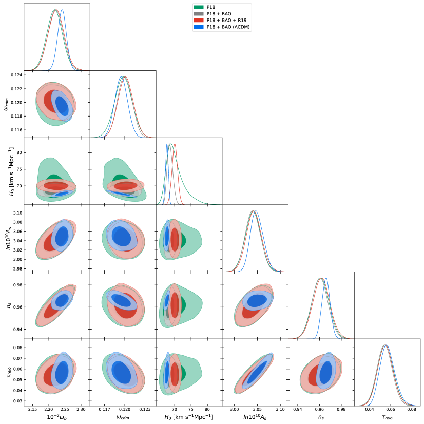
Figure 15: Marginalized joint 68% and 95% CL regions 2D parameter space using the $Planck$ legacy data (green), its combination with BAO DR12, i.e. P18 + BAO (gray), and P18 + BAO + R19 (red) for the IG model. We include the contours for the $\Lambda$CDM in blue for P18 + BAO.

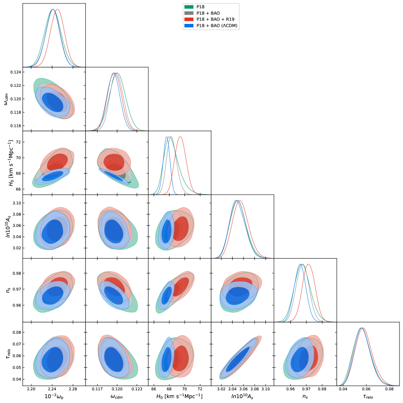
Figure 16: Marginalized joint 68% and 95% CL regions 2D parameter space using the $Planck$ legacy data (green), its combination with BAO DR12, i.e. P18 + BAO (gray), and P18 + BAO + R19 (red) for the CC model. We include the contours for the $\Lambda$CDM in blue for P18 + BAO.

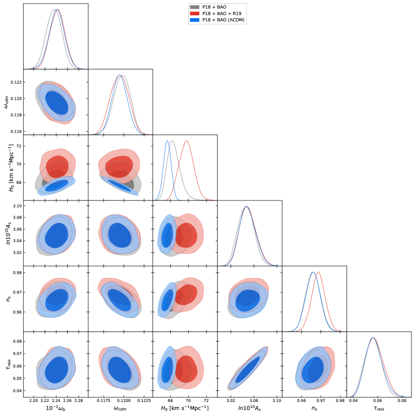
Figure 17: Marginalized joint 68% and 95% CL regions 2D parameter space using the $Planck$ legacy data in combination with BAO DR12 (gray) and P18 + BAO + R19 (red) for the NMC+ model. We include the contours for the $\Lambda$CDM in blue for P18 + BAO.

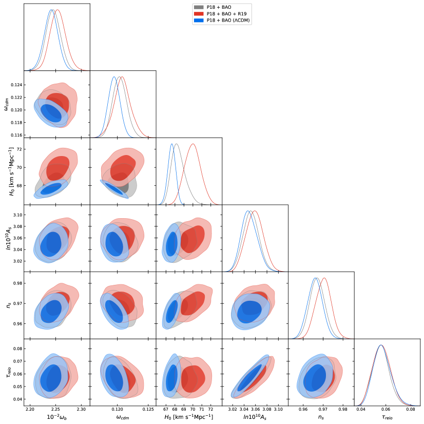
Figure 18: Marginalized joint 68% and 95% CL regions 2D parameter space using the $Planck$ legacy data in combination with BAO DR12 (gray) and P18 + BAO + R19 (red) for the NMC- model. We include the contours for the $\Lambda$CDM in blue for P18 + BAO.

References

- Uzan [2003] Jean-Philippe Uzan. The Fundamental Constants and Their Variation: Observational Status and Theoretical Motivations. Rev. Mod. Phys., 75:403, 2003. doi: 10.1103/RevModPhys.75.403.
- Dirac [1937] Paul A. M. Dirac. The Cosmological constants. Nature, 139:323, 1937. doi: 10.1038/139323a0.
- Will [2006] Clifford M. Will. The Confrontation between general relativity and experiment. Living Rev. Rel., 9:3, 2006. doi: 10.12942/lrr-2006-3.
- Bertotti et al. [2003] B. Bertotti, L. Iess, and P. Tortora. A test of general relativity using radio links with the Cassini spacecraft. Nature, 425:374–376, 2003. doi: 10.1038/nature01997.
- Will [2014] Clifford M. Will. The Confrontation between General Relativity and Experiment. Living Rev. Rel., 17:4, 2014. doi: 10.12942/lrr-2014-4.
- Muller and Biskupek [2007] Jurgen Muller and Liliane Biskupek. Variations of the gravitational constant from lunar laser ranging data. Class. Quant. Grav., 24:4533–4538, 2007. doi: 10.1088/0264-9381/24/17/017.
- Garcia-Berro et al. [2011] Enrique Garcia-Berro, Pablo Loren-Aguilar, Santiago Torres, Leandro G. Althaus, and Jordi Isern. An upper limit to the secular variation of the gravitational constant from white dwarf stars. JCAP, 05:021, 2011. doi: 10.1088/1475-7516/2011/05/021.
- Mould and Uddin [2014] Jeremy Mould and Syed Uddin. Constraining a possible variation of G with Type Ia supernovae. Publ. Astron. Soc. Austral., 31:15, 2014. doi: 10.1017/pasa.2014.9.
- Bellinger and Christensen-Dalsgaard [2019] Earl Patrick Bellinger and Jørgen Christensen-Dalsgaard. Asteroseismic constraints on the cosmic-time variation of the gravitational constant from an ancient main-sequence star. Astrophys. J. Lett., 887(1):L1, 2019. doi: 10.3847/2041-8213/ab43e7.
- Zhu et al. [2019] W. W. Zhu et al. Tests of Gravitational Symmetries with Pulsar Binary J1713+0747. Mon. Not. Roy. Astron. Soc., 482(3):3249–3260, 2019. doi: 10.1093/mnras/sty2905.
- Casas et al. [1992a] J. A. Casas, J. Garcia-Bellido, and M. Quiros. Nucleosynthesis bounds on Jordan-Brans-Dicke theories of gravity. Mod. Phys. Lett. A, 7:447–456, 1992a. doi: 10.1142/S0217732392000409.
- Casas et al. [1992b] J. A. Casas, J. Garcia-Bellido, and M. Quiros. Updating nucleosynthesis bounds on Jordan-Brans-Dicke theories of gravity. Phys. Lett. B, 278:94–96, 1992b. doi: 10.1016/0370-2693(92)90717-I.
- Santiago et al. [1997] D. I. Santiago, D. Kalligas, and R. V. Wagoner. Nucleosynthesis constraints on scalar - tensor theories of gravity. Phys. Rev. D, 56:7627–7637, 1997. doi: 10.1103/PhysRevD.56.7627.
- Clifton et al. [2005] Timothy Clifton, John D. Barrow, and Robert J. Scherrer. Constraints on the variation of G from primordial nucleosynthesis. Phys. Rev. D, 71:123526, 2005. doi: 10.1103/PhysRevD.71.123526.
- Bambi et al. [2005] Cosimo Bambi, Maurizio Giannotti, and F. L. Villante. The Response of primordial abundances to a general modification of G(N) and/or of the early Universe expansion rate. Phys. Rev. D, 71:123524, 2005. doi: 10.1103/PhysRevD.71.123524.
- Copi et al. [2004] Craig J. Copi, Adam N. Davis, and Lawrence M. Krauss. A New nucleosynthesis constraint on the variation of G. Phys. Rev. Lett., 92:171301, 2004. doi: 10.1103/PhysRevLett.92.171301.
- Alvey et al. [2020] James Alvey, Nashwan Sabti, Miguel Escudero, and Malcolm Fairbairn. Improved BBN Constraints on the Variation of the Gravitational Constant. Eur. Phys. J. C, 80(2):148, 2020. doi: 10.1140/epjc/s10052-020-7727-y.
- Aghanim et al. [2020a] N. Aghanim et al. Planck 2018 results. VI. Cosmological parameters. Astron. Astrophys., 641:A6, 2020a. doi: 10.1051/0004-6361/201833910.
- Umezu et al. [2005] Ken-ichi Umezu, Kiyotomo Ichiki, and Masanobu Yahiro. Cosmological constraints on Newton’s constant. Phys. Rev. D, 72:044010, 2005. doi: 10.1103/PhysRevD.72.044010.
- Chang and Chu [2007] Kwan-Chuen Chang and M. C. Chu. Constraining the Variation of G by Cosmic Microwave Background Anisotropies. Phys. Rev. D, 75:083521, 2007. doi: 10.1103/PhysRevD.75.083521.
- Perenon et al. [2019] Louis Perenon, Julien Bel, Roy Maartens, and Alvaro de la Cruz-Dombriz. Optimising growth of structure constraints on modified gravity. JCAP, 06:020, 2019. doi: 10.1088/1475-7516/2019/06/020.
- Hanımeli et al. [2020] Ekim Taylan Hanımeli, Brahim Lamine, Alain Blanchard, and Isaac Tutusaus. Time-dependent in Einstein’s equations as an alternative to the cosmological constant. Phys. Rev. D, 101(6):063513, 2020. doi: 10.1103/PhysRevD.101.063513.
- Sapone et al. [2021] Domenico Sapone, Savvas Nesseris, and Carlos A. P. Bengaly. Is there any measurable redshift dependence on the SN Ia absolute magnitude? Phys. Dark Univ., 32:100814, 2021. doi: 10.1016/j.dark.2021.100814.
- Sakr and Sapone [2021] Ziad Sakr and Domenico Sapone. Can varying the gravitational constant alleviate the tensions? 12 2021. arXiv:2112.14173.
- Zahn and Zaldarriaga [2003] Oliver Zahn and Matias Zaldarriaga. Probing the Friedmann equation during recombination with future CMB experiments. Phys. Rev. D, 67:063002, 2003. doi: 10.1103/PhysRevD.67.063002.
- Galli et al. [2009] Silvia Galli, Alessandro Melchiorri, George F. Smoot, and Oliver Zahn. From Cavendish to PLANCK: Constraining Newton’s Gravitational Constant with CMB Temperature and Polarization Anisotropy. Phys. Rev. D, 80:023508, 2009. doi: 10.1103/PhysRevD.80.023508.
- Martins et al. [2010] C. J. A. P. Martins, Eloisa Menegoni, Silvia Galli, Gianpiero Mangano, and Alessandro Melchiorri. Varying couplings in the early universe: correlated variations of and . Phys. Rev. D, 82:023532, 2010. doi: 10.1103/PhysRevD.82.023532.
- Ballardini et al. [2020] Mario Ballardini, Matteo Braglia, Fabio Finelli, Daniela Paoletti, Alexei A. Starobinsky, and Caterina Umiltà. Scalar-tensor theories of gravity, neutrino physics, and the tension. JCAP, 10:044, 2020. doi: 10.1088/1475-7516/2020/10/044.
- Paoletti et al. [2019] D. Paoletti, M. Braglia, F. Finelli, M. Ballardini, and C. Umiltà. Isocurvature fluctuations in the effective Newton’s constant. Phys. Dark Univ., 25:100307, 2019. doi: 10.1016/j.dark.2019.100307.
- Umiltà et al. [2015] C. Umiltà, M. Ballardini, F. Finelli, and D. Paoletti. CMB and BAO constraints for an induced gravity dark energy model with a quartic potential. JCAP, 08:017, 2015. doi: 10.1088/1475-7516/2015/08/017.
- Ballardini et al. [2016a] Mario Ballardini, Fabio Finelli, Caterina Umiltà, and Daniela Paoletti. Cosmological constraints on induced gravity dark energy models. JCAP, 05:067, 2016a. doi: 10.1088/1475-7516/2016/05/067.
- Rossi et al. [2019] Massimo Rossi, Mario Ballardini, Matteo Braglia, Fabio Finelli, Daniela Paoletti, Alexei A. Starobinsky, and Caterina Umiltà. Cosmological constraints on post-Newtonian parameters in effectively massless scalar-tensor theories of gravity. Phys. Rev. D, 100(10):103524, 2019. doi: 10.1103/PhysRevD.100.103524.
- Schöneberg et al. [2021] Nils Schöneberg, Guillermo Franco Abellán, Andrea Pérez Sánchez, Samuel J. Witte, Vivian Poulin, and Julien Lesgourgues. The Olympics: A fair ranking of proposed models. 7 2021. arXiv: 2107.10291.
- Di Valentino et al. [2021] Eleonora Di Valentino et al. Snowmass2021 - Letter of interest cosmology intertwined II: The hubble constant tension. Astropart. Phys., 131:102605, 2021. doi: 10.1016/j.astropartphys.2021.102605.
- Marra and Perivolaropoulos [2021] Valerio Marra and Leandros Perivolaropoulos. Rapid transition of Geff at zt0.01 as a possible solution of the Hubble and growth tensions. Phys. Rev. D, 104(2):L021303, 2021. doi: 10.1103/PhysRevD.104.L021303.
- Alestas et al. [2021] George Alestas, David Camarena, Eleonora Di Valentino, Lavrentios Kazantzidis, Valerio Marra, Savvas Nesseris, and Leandros Perivolaropoulos. Late-transition vs smooth deformation models for the resolution of the Hubble crisis. 10 2021. arXiv: 2110.04336.
- Jordan [1949] Pascual Jordan. Formation of the Stars and Development of the Universe. Nature, 164:637–640, 1949. doi: 10.1038/164637a0.
- Brans and Dicke [1961] C. Brans and R. H. Dicke. Mach’s principle and a relativistic theory of gravitation. Phys. Rev., 124:925–935, 1961. doi: 10.1103/PhysRev.124.925.
- Chen and Kamionkowski [1999] Xue-lei Chen and Marc Kamionkowski. Cosmic microwave background temperature and polarization anisotropy in Brans-Dicke cosmology. Phys. Rev. D, 60:104036, 1999. doi: 10.1103/PhysRevD.60.104036.
- Nagata et al. [2004] Ryo Nagata, Takeshi Chiba, and Naoshi Sugiyama. WMAP constraints on scalar- tensor cosmology and the variation of the gravitational constant. Phys. Rev. D, 69:083512, 2004. doi: 10.1103/PhysRevD.69.083512.
- Acquaviva et al. [2005] Viviana Acquaviva, Carlo Baccigalupi, Samuel M. Leach, Andrew R. Liddle, and Francesca Perrotta. Structure formation constraints on the Jordan-Brans-Dicke theory. Phys. Rev. D, 71:104025, 2005. doi: 10.1103/PhysRevD.71.104025.
- Li et al. [2013] Yi-Chao Li, Feng-Quan Wu, and Xuelei Chen. Constraints on the Brans-Dicke gravity theory with the Planck data. Phys. Rev. D, 88:084053, 2013. doi: 10.1103/PhysRevD.88.084053.
- Avilez and Skordis [2014] A. Avilez and C. Skordis. Cosmological constraints on Brans-Dicke theory. Phys. Rev. Lett., 113(1):011101, 2014. doi: 10.1103/PhysRevLett.113.011101.
- Ooba et al. [2016] Junpei Ooba, Kiyotomo Ichiki, Takeshi Chiba, and Naoshi Sugiyama. Planck constraints on scalar-tensor cosmology and the variation of the gravitational constant. Phys. Rev. D, 93(12):122002, 2016. doi: 10.1103/PhysRevD.93.122002.
- Ooba et al. [2017] Junpei Ooba, Kiyotomo Ichiki, Takeshi Chiba, and Naoshi Sugiyama. Cosmological constraints on scalar–tensor gravity and the variation of the gravitational constant. PTEP, 2017(4):043E03, 2017. doi: 10.1093/ptep/ptx046.
- Solà Peracaula et al. [2019] Joan Solà Peracaula, Adria Gomez-Valent, Javier de Cruz Pérez, and Cristian Moreno-Pulido. Brans–Dicke Gravity with a Cosmological Constant Smoothes Out CDM Tensions. Astrophys. J. Lett., 886(1):L6, 2019. doi: 10.3847/2041-8213/ab53e9.
- Ballesteros et al. [2020] Guillermo Ballesteros, Alessio Notari, and Fabrizio Rompineve. The tension: vs. . JCAP, 11:024, 2020. doi: 10.1088/1475-7516/2020/11/024.
- Braglia et al. [2020] Matteo Braglia, Mario Ballardini, William T. Emond, Fabio Finelli, A. Emir Gumrukcuoglu, Kazuya Koyama, and Daniela Paoletti. Larger value for by an evolving gravitational constant. Phys. Rev. D, 102(2):023529, 2020. doi: 10.1103/PhysRevD.102.023529.
- Braglia et al. [2021] Matteo Braglia, Mario Ballardini, Fabio Finelli, and Kazuya Koyama. Early modified gravity in light of the tension and LSS data. Phys. Rev. D, 103(4):043528, 2021. doi: 10.1103/PhysRevD.103.043528.
- Cheng et al. [2021] Gong Cheng, Fengquan Wu, and Xuelei Chen. Cosmological test of an extended quintessence model. Phys. Rev. D, 103(10):103527, 2021. doi: 10.1103/PhysRevD.103.103527.
- Joudaki et al. [2020] Shahab Joudaki, Pedro G. Ferreira, Nelson A. Lima, and Hans A. Winther. Testing Gravity on Cosmic Scales: A Case Study of Jordan-Brans-Dicke Theory. 10 2020. arXiv: 2010.15278.
- Amendola [1999] Luca Amendola. Scaling solutions in general nonminimal coupling theories. Phys. Rev. D, 60:043501, 1999. doi: 10.1103/PhysRevD.60.043501.
- Finelli et al. [2008] F. Finelli, A. Tronconi, and Giovanni Venturi. Dark Energy, Induced Gravity and Broken Scale Invariance. Phys. Lett. B, 659:466–470, 2008. doi: 10.1016/j.physletb.2007.11.053.
- Boisseau et al. [2000] B. Boisseau, Gilles Esposito-Farese, D. Polarski, and Alexei A. Starobinsky. Reconstruction of a scalar tensor theory of gravity in an accelerating universe. Phys. Rev. Lett., 85:2236, 2000. doi: 10.1103/PhysRevLett.85.2236.
- Gannouji et al. [2006] Radouane Gannouji, David Polarski, Andre Ranquet, and Alexei A. Starobinsky. Scalar-Tensor Models of Normal and Phantom Dark Energy. JCAP, 09:016, 2006. doi: 10.1088/1475-7516/2006/09/016.
- Audren et al. [2013] Benjamin Audren, Julien Lesgourgues, Karim Benabed, and Simon Prunet. Conservative Constraints on Early Cosmology: an illustration of the Monte Python cosmological parameter inference code. JCAP, 02:001, 2013. doi: 10.1088/1475-7516/2013/02/001.
- Brinckmann and Lesgourgues [2019] Thejs Brinckmann and Julien Lesgourgues. MontePython 3: boosted MCMC sampler and other features. Phys. Dark Univ., 24:100260, 2019. doi: 10.1016/j.dark.2018.100260.
- Lesgourgues [2011] Julien Lesgourgues. The Cosmic Linear Anisotropy Solving System (CLASS) I: Overview. 4 2011. arXiv: 1104.2932.
- Blas et al. [2011] Diego Blas, Julien Lesgourgues, and Thomas Tram. The Cosmic Linear Anisotropy Solving System (CLASS) II: Approximation schemes. JCAP, 07:034, 2011. doi: 10.1088/1475-7516/2011/07/034.
- Lewis [2019] Antony Lewis. GetDist: a Python package for analysing Monte Carlo samples. 10 2019.
- Pisanti et al. [2008] O. Pisanti, A. Cirillo, S. Esposito, F. Iocco, G. Mangano, G. Miele, and P. D. Serpico. PArthENoPE: Public Algorithm Evaluating the Nucleosynthesis of Primordial Elements. Comput. Phys. Commun., 178:956–971, 2008. doi: 10.1016/j.cpc.2008.02.015.
- Consiglio et al. [2018] R. Consiglio, P. F. de Salas, G. Mangano, G. Miele, S. Pastor, and O. Pisanti. PArthENoPE reloaded. Comput. Phys. Commun., 233:237–242, 2018. doi: 10.1016/j.cpc.2018.06.022.
- Hamann et al. [2008] Jan Hamann, Julien Lesgourgues, and Gianpiero Mangano. Using BBN in cosmological parameter extraction from CMB: A Forecast for PLANCK. JCAP, 03:004, 2008. doi: 10.1088/1475-7516/2008/03/004.
- Reid et al. [2019] M. J. Reid, D. W. Pesce, and A. G. Riess. An Improved Distance to NGC 4258 and its Implications for the Hubble Constant. Astrophys. J. Lett., 886(2):L27, 2019. doi: 10.3847/2041-8213/ab552d.
- Aghanim et al. [2020b] N. Aghanim et al. Planck 2018 results. V. CMB power spectra and likelihoods. Astron. Astrophys., 641:A5, 2020b. doi: 10.1051/0004-6361/201936386.
- Aghanim et al. [2020c] N. Aghanim et al. Planck 2018 results. VIII. Gravitational lensing. Astron. Astrophys., 641:A8, 2020c. doi: 10.1051/0004-6361/201833886.
- Alam et al. [2017a] Shadab Alam et al. The clustering of galaxies in the completed SDSS-III Baryon Oscillation Spectroscopic Survey: cosmological analysis of the DR12 galaxy sample. Mon. Not. Roy. Astron. Soc., 470(3):2617–2652, 2017a. doi: 10.1093/mnras/stx721.
- Beutler et al. [2011] Florian Beutler, Chris Blake, Matthew Colless, D. Heath Jones, Lister Staveley-Smith, Lachlan Campbell, Quentin Parker, Will Saunders, and Fred Watson. The 6dF Galaxy Survey: Baryon Acoustic Oscillations and the Local Hubble Constant. Mon. Not. Roy. Astron. Soc., 416:3017–3032, 2011. doi: 10.1111/j.1365-2966.2011.19250.x.
- Ross et al. [2015] Ashley J. Ross, Lado Samushia, Cullan Howlett, Will J. Percival, Angela Burden, and Marc Manera. The clustering of the SDSS DR7 main Galaxy sample – I. A 4 per cent distance measure at . Mon. Not. Roy. Astron. Soc., 449(1):835–847, 2015. doi: 10.1093/mnras/stv154.
- Abbott et al. [2018] T. M. C. Abbott et al. Dark Energy Survey year 1 results: Cosmological constraints from galaxy clustering and weak lensing. Phys. Rev. D, 98(4):043526, 2018. doi: 10.1103/PhysRevD.98.043526.
- Hildebrandt et al. [2017] H. Hildebrandt et al. KiDS-450: Cosmological parameter constraints from tomographic weak gravitational lensing. Mon. Not. Roy. Astron. Soc., 465:1454, 2017. doi: 10.1093/mnras/stw2805.
- Hildebrandt et al. [2020] H. Hildebrandt et al. KiDS+VIKING-450: Cosmic shear tomography with optical and infrared data. Astron. Astrophys., 633:A69, 2020. doi: 10.1051/0004-6361/201834878.
- Hikage et al. [2019] Chiaki Hikage et al. Cosmology from cosmic shear power spectra with Subaru Hyper Suprime-Cam first-year data. Publ. Astron. Soc. Jap., 71(2):43, 2019. doi: 10.1093/pasj/psz010.
- Hazumi et al. [2020] M. Hazumi et al. LiteBIRD: JAXA’s new strategic L-class mission for all-sky surveys of cosmic microwave background polarization. Proc. SPIE Int. Soc. Opt. Eng., 11443:114432F, 2020. doi: 10.1117/12.2563050.
- Abazajian et al. [2019] Kevork Abazajian et al. CMB-S4 Science Case, Reference Design, and Project Plan. 7 2019. arXiv: 1907.04473.
- Benson et al. [2014] B. A. Benson et al. SPT-3G: A Next-Generation Cosmic Microwave Background Polarization Experiment on the South Pole Telescope. Proc. SPIE Int. Soc. Opt. Eng., 9153:91531P, 2014. doi: 10.1117/12.2057305.
- Ade et al. [2019] Peter Ade et al. The Simons Observatory: Science goals and forecasts. JCAP, 02:056, 2019. doi: 10.1088/1475-7516/2019/02/056.
- Ballardini et al. [2019] M. Ballardini, D. Sapone, C. Umiltà, F. Finelli, and D. Paoletti. Testing extended Jordan-Brans-Dicke theories with future cosmological observations. JCAP, 05:049, 2019. doi: 10.1088/1475-7516/2019/05/049.
- Hu and Okamoto [2002] Wayne Hu and Takemi Okamoto. Mass reconstruction with cmb polarization. Astrophys. J., 574:566–574, 2002. doi: 10.1086/341110.
- Hirata and Seljak [2003] Christopher M. Hirata and Uros Seljak. Reconstruction of lensing from the cosmic microwave background polarization. Phys. Rev. D, 68:083002, 2003. doi: 10.1103/PhysRevD.68.083002.
- Smith et al. [2012] Kendrick M. Smith, Duncan Hanson, Marilena LoVerde, Christopher M. Hirata, and Oliver Zahn. Delensing CMB Polarization with External Datasets. JCAP, 06:014, 2012. doi: 10.1088/1475-7516/2012/06/014.
- Seo and Eisenstein [2003] Hee-Jong Seo and Daniel J. Eisenstein. Probing dark energy with baryonic acoustic oscillations from future large galaxy redshift surveys. Astrophys. J., 598:720–740, 2003. doi: 10.1086/379122.
- Song and Percival [2009] Yong-Seon Song and Will J. Percival. Reconstructing the history of structure formation using Redshift Distortions. JCAP, 10:004, 2009. doi: 10.1088/1475-7516/2009/10/004.
- Wang et al. [2013] Yun Wang, Chia-Hsun Chuang, and Christopher M. Hirata. Toward More Realistic Forecasting of Dark Energy Constraints from Galaxy Redshift Surveys. Mon. Not. Roy. Astron. Soc., 430:2446, 2013. doi: 10.1093/mnras/stt068.
- Blanchard et al. [2020] A. Blanchard et al. Euclid preparation: VII. Forecast validation for Euclid cosmological probes. Astron. Astrophys., 642:A191, 2020. doi: 10.1051/0004-6361/202038071.
- Alcock and Paczynski [1979] C. Alcock and B. Paczynski. An evolution free test for non-zero cosmological constant. Nature, 281:358–359, 1979. doi: 10.1038/281358a0.
- Kaiser [1987] N. Kaiser. Clustering in real space and in redshift space. Mon. Not. Roy. Astron. Soc., 227:1–27, 1987.
- Boyle and Komatsu [2018] Aoife Boyle and Eiichiro Komatsu. Deconstructing the neutrino mass constraint from galaxy redshift surveys. JCAP, 03:035, 2018. doi: 10.1088/1475-7516/2018/03/035.
- Aghamousa et al. [2016] Amir Aghamousa et al. The DESI Experiment Part I: Science,Targeting, and Survey Design. 10 2016. arXiv: 1611.00036.
- Ballardini et al. [2016b] Mario Ballardini, Fabio Finelli, Cosimo Fedeli, and Lauro Moscardini. Probing primordial features with future galaxy surveys. JCAP, 10:041, 2016b. doi: 10.1088/1475-7516/2016/10/041. [Erratum: JCAP 04, E01 (2018)].
- Alam et al. [2017b] Shadab Alam et al. The clustering of galaxies in the completed SDSS-III Baryon Oscillation Spectroscopic Survey: cosmological analysis of the DR12 galaxy sample. Mon. Not. Roy. Astron. Soc., 470(3):2617–2652, 2017b. doi: 10.1093/mnras/stx721.
- Amendola et al. [2008] Luca Amendola, Martin Kunz, and Domenico Sapone. Measuring the dark side (with weak lensing). JCAP, 04:013, 2008. doi: 10.1088/1475-7516/2008/04/013.
- Majerotto et al. [2016] Elisabetta Majerotto, Domenico Sapone, and Björn Malte Schäfer. Combined constraints on deviations of dark energy from an ideal fluid from Euclid and Planck. Mon. Not. Roy. Astron. Soc., 456(1):109–118, 2016. doi: 10.1093/mnras/stv2640.
- Palma et al. [2018] Gonzalo A. Palma, Domenico Sapone, and Spyros Sypsas. Constraints on inflation with LSS surveys: features in the primordial power spectrum. JCAP, 06:004, 2018. doi: 10.1088/1475-7516/2018/06/004.
- Schaan et al. [2017] Emmanuel Schaan, Elisabeth Krause, Tim Eifler, Olivier Doré, Hironao Miyatake, Jason Rhodes, and David N. Spergel. Looking through the same lens: Shear calibration for LSST, Euclid, and WFIRST with stage 4 CMB lensing. Phys. Rev. D, 95(12):123512, 2017. doi: 10.1103/PhysRevD.95.123512.
- Mandelbaum et al. [2018] Rachel Mandelbaum et al. The LSST Dark Energy Science Collaboration (DESC) Science Requirements Document. 9 2018. arXiv: 1809.01669.
- Tassev et al. [2013] Svetlin Tassev, Matias Zaldarriaga, and Daniel Eisenstein. Solving Large Scale Structure in Ten Easy Steps with COLA. JCAP, 06:036, 2013. doi: 10.1088/1475-7516/2013/06/036.
- Winther et al. [2017] Hans A. Winther, Kazuya Koyama, Marc Manera, Bill S. Wright, and Gong-Bo Zhao. COLA with scale-dependent growth: applications to screened modified gravity models. JCAP, 08:006, 2017. doi: 10.1088/1475-7516/2017/08/006.
- Alonso et al. [2017] David Alonso, Emilio Bellini, Pedro G. Ferreira, and Miguel Zumalacárregui. Observational future of cosmological scalar-tensor theories. Phys. Rev. D, 95(6):063502, 2017. doi: 10.1103/PhysRevD.95.063502.