Multi-Robot Object Transport Motion Planning with a Deformable Sheet
Abstract
Using a deformable sheet to handle objects is convenient and found in many practical applications. For object manipulation through a deformable sheet that is held by multiple mobile robots, it is a challenging task to model the object-sheet interactions. We present a computational model and algorithm to capture the object position on the deformable sheet with changing robotic team formations. A virtual variable cables model (VVCM) is proposed to simplify the modeling of the robot-sheet-object system. With the VVCM, we further present a motion planner for the robotic team to transport the object in a three-dimensional (3D) cluttered environment. Simulation and experimental results with different robot team sizes show the effectiveness and versatility of the proposed VVCM. We also compare and demonstrate the planning results to avoid the obstacle in 3D space with the other benchmark planner.
Index Terms:
Multi-robot manipulation, collaborative manipulation, multi-robot motion planning.I Introduction
Deformable sheets are commonly used as flexible carriers in many object manipulation applications, such as transferring patients with bed sheets in hospital [1]. Due to sheet deformability, multiple supporters (e.g., mobile robots) are needed to carry the object in the sheet. For robot-sheet-object transport systems, sheet deformability provides an advantage of manipulating objects by changing the relative positions among the robotic team members. However, this feature also brings challenges for real-time modeling of the object-sheet interactions, robot formation control and motion planning. The goal of this paper is to present an efficient computational approach for multi-robot motion planning for manipulating and transporting an object in a deformable sheet held by the robotic team.
Using a mobile robot team to collaboratively transport or manipulate a rigid object has been reported in previous decades. By different contact methods, multi-robot manipulation (MRM) can be classified into three types: pushing, grasping, and caging [2]. In these systems, robots are in direct contact with the transported or manipulated objects. The work in [3] proposed a distributed multi-mobile robot control method to transport a rigid object. The fixed formation shape did not allow the robot team to adjust relative positions between any two robots for obstacle avoidance in cluttered environment, such as narrow passes. For multi-mobile manipulators, Ren et al. [4] presented a fully distributed control scheme for a team of networked mobile manipulators to transport an unknown object. The manipulator is expensive and its kinematic redundancy also brings additional planning and control design challenges.
Using deformable sheets to hold an object provides a new way for MRM. The motion of objects on the sheet is highly dependent on the robot motion and is not easily predicted due to high dimensionality of deformable sheets [5]. Physical and geometric models are among the main modeling methods of the deformable sheet [6]. Physical models such as the mass-spring model [7] and finite element method [8] are common in computer graphics. The work in [9] studied a set of cloth manipulation tasks in daily activities, including folding laundry, wringing a towel, and putting on a scarf. The motion between the rigid body and the cloth was calculated by a physics-based simulator, which involves complex meshing and calculations and cannot be used for real-time applications.
In robotic manipulation, geometric models are used to reduce the high dimensionality of the sheet. In [10, 11], the geometric constraints of the deformable sheet are used for motion planning without the complete model. The work in [12] used a set of discrete points to approximate the sheet state. Assuming a completely flexible sheet, the work in [13, 14] established the geometric link model of the sheet-object kinematic relationship with a three-robot team. The recent work in [15] extended the sheet-object kinematic model to include rotational motion of a spherical-shape object for pose manipulation. As the number of robots increases, the transported object may have different equilibrium states on the sheet, and the the physical principle-based kinematic models developed in [14, 15] becomes complicated and difficult to obtain precisely.
Inspired by the configuration of cable suspended robots [16, 17, 18], we propose the virtual variable cables model (VVCM) that simplifies the object-sheet interactions as a set of dynamically changing cables to collaboratively hold the object. The equilibrium of the object on the sheet is then represented by the tightness status of virtual cables in the quasi-static state. A computational algorithm is proposed for obtaining real-time object position in the sheet that is held by arbitrary numbers of mobile robots. Based on the VVCM, we also propose a motion planner for the robotic team for manipulating and transporting the object in cluttered environment. It is difficult to use the artificial potential field method [19] or sampling-based planning algorithms [20] to maintain the shape of the multi-robot formation. Alonso et al. [21] computed the optimal robotic formation through a constrained nonlinear optimization problem for multi-mobile manipulator-base object manipulation with the deformable sheet. The motion planners in [10, 11, 12, 13, 14, 21] did not consider the three-dimensional (3D) position of the transported object with deformable sheets. For obstacle avoidance, the object is always planned to bypass the obstacle, that is, planar motion in two-dimensional (2D) space. Our planner is an extension of these planners and we exploit the possible obstacle avoidance in 3D space by allowing the object to move above the obstacles, which is referred as obstacle crossing. Therefore, the proposed motion planner allows the robotic team to avoid obstacles in both 2D or 3D space, which is efficient and effective in cluttered environments (e.g., a narrow corridor with obstacles).
The main contributions of this paper are twofold. First, the proposed VVCM for robots-sheet-object interactions is new and provides an efficient method to compute the different equilibrium of the object on the sheet held by arbitrary number of robots. Second, the motion planning algorithm extends the existing planners for MRM with the new capability of obstacle crossing, which not only expands the workspace of the robot team, but also improves the efficiency.
The remainder of this paper is organized as follows. We first present the problem statement in Section II. Section III presents the computational model for object manipulation with a deformable sheet. Section IV discusses the motion planner with obstacle crossing capability. Section V presents the experimental results and finally, Section VI summarizes the concluding remarks.
II System Configuration and Problem Statement
II-A System Configuration
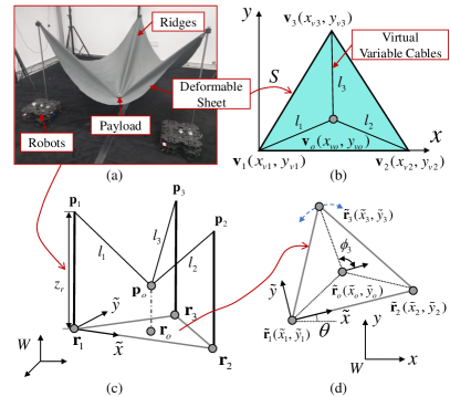
We consider the object manipulation and transporting by a deformable sheet that is held by mobile robots, . Fig. 1(a) illustrates the system configuration for a three-robot case, that is, . The trajectory of the transported object, denoted as , is in 3D space and the mobile robots only move on the planar surface. A deformable sheet is held by an -mobile robot team and the robotic holding point , , is fixed at a constant height.
To describe the motion of object on the deformable sheet, we consider the local sheet frame, denoted as , on the plat sheet plane. The coordinate of points on is denoted as , . The contact point between object and the sheet is denoted as in , as shown in Fig. 1(b). A world coordinate frame is also used and the coordinate of is denoted as , , , where is a constant height for all robots. The coordinate of object in as . Fig. 1(c) further illustrates the coordinates of and . The collection of all robots’ position is denoted as .
The motion of the object is closely related to the robot motion and the material and shape of the sheet. To precisely describe the motion and restrict the problem scope, we use the following considerations and assumptions. First, the object is assumed to be a mass point. Second, the object transport and motion are quasi-static, that is, the robot team moves slowly and smoothly and the dynamic effects of object ’s motion are negligible. Finally, the deformable sheet is completely soft and inelastic and thus, the object moves freely on the sheet under gravity. With these considerations, the sheet holding points in form a convex polygon with vertices and the object is located inside the polygon; see Fig. 1(b) for a triangle case (i.e., ). It is clear that in non-constrained conditions, the object tends to move and stay at the position of minimum potential energy.
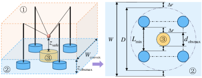
The 3D position of object is directly related to the shape of the robot formation. Fig. 2 illustrates the multi-robot formation configuration. The object is considered to be transported by the robotic team in a space with width ; see the left plot of Fig. 2. To quantify the formation properties, we introduce a few geometric variables that will be used later in motion planning design, including the robotic formation size , the maximum traversable obstacle height and the maximum traversable obstacle diameter .
The robotic formation size is defined as
| (1) |
where is the diameter of the minimum circumscribed circle of the robotic team and is a constant safety distance at each side of the robotic formation; see Fig 2. The maximum traversable obstacle height is obtained as
| (2) |
where is a minimum safety distance between the object and the obstacle. We assume that each robot is a particle and we define the shortest distance between any two robots as
| (3) |
where index set . The maximum traversable obstacle diameter is then defined as
| (4) |
From (2)-(4), variables , and are the functions of formation shape that is determined by and we will use these variables to design motion planner in Section IV.
II-B Problem Statement
One important observation of the object in the deformable sheet that is held by points is that the connection between and in frame can be a straight-line (i.e., full tension) or a curved-line (i.e., slack). We call the connected line between and on as ridge. By the local coordinates in frame , the geodesic length of the th ridge is denoted as , . The planar position of the th robot is captured by . We assume that the initial position of all robots and obstacles in 3D space are known. The problem statement is given as follows.
Problem Statement: The motion planning problem is to design the trajectory of robot team such that the object can be safely transport from the initial to target positions in 3D space.
III Multi-Robot Manipulation Models
In this section, we present a computational approach to obtain the object position under the motion of the robotic team. The goal of the multi-robot manipulation model is to compute object positions for given .
III-A Virtual Variable Cables Model (VVCM)
Due to the inelastic property, the sheet deformation is distance-preserving. As the robot formation changes, the object might move on the sheet under gravity and therefore, the contact point also changes. Since the geodesic distance between and on varies, the th ridge can be viewed as a virtual cable connecting points and ; see Fig. 1(c). Therefore, the object can be regarded as being transported by variable-length cables that are fixed on the robot. Because the virtual cable might be taut or slack, it is clear that the Euclidean distance between object and vertex is less than or equal to the corresponding virtual cable length, namely,
| (5) |
The complexity of the above described virtual cable-object interactions lies in the unspecified taut/slack status of each cable under robot formation. The positions of the object are jointly determined by the set of taut cables. To precisely determine the object position, we define the status of the th virtual cable by variable if the cable is slack; otherwise, when it is taut, . Furthermore, defining taut cable index set , we denote as the cardinality of . When the th cable is taut (i.e., ), it satisfies
| (6) |
The direct kinematics is to know the robotic formation to solve the positions of the object . To obtain an algebraic solution, the formation can be transformed into a local coordinate system, as shown in Fig. 1(d). In the local coordinate system, with as the origin and as the -axis, the robots’ coordinates are arranged in counterclockwise order, denoted as . The projected coordinate of the transported object is denoted as in the local frame. The direct kinematics can be simplified as that given , , and by the above setup, we need to find and , which consists of five independent coordinate variables of the transported object.
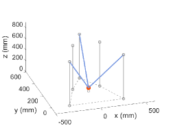
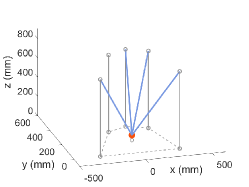
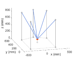
For the VVCM with an -robot team, different combinations of the taut virtual cables represent different geometric constraints. Because of the above-mentioned five independent variables, we use 5-robot team as an illustrative example to determine possible equilibrium conditions of the transported object. Fig. 3 illustrates three possible equilibrium state of the object under a five-robot team. Among five virtual cables, the numbers of taut cables can be 3, 4, or 5 as illustrated in Fig. 3(a)-(c), respectively.
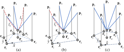
The projection of , , on the local frame must be convex polygons; otherwise, the th virtual cable must be slack, that is, , which results in a change of the object’s equilibrium state. We first consider the case when five cables are taut, i.e., , as shown in Fig. 3(c). In this case, all five cables satisfy the geometric constraints (6). Through these five independent equations, the required five independent variables can be obtained. The calculation function is denoted as VVCM-Pentagon as shown in the computational approach with pseudo-code illustrated in Algorithm 1. When more than five cables are taut in a larger robot team, , the object is constrained by full redundancy and its position is determined by any five independent equations in the geometric constraints (6). Therefore, we can obtain by selecting five taut cables from the team.
Fig. 3(a) shows the case when two cables are slack and the object’s position is determined by the triangle sub-formation. The configuration is considered as a three-robot team, , similar to that as shown in Fig. 1. In this case, combining the three geometric constraint equations (6) in the local coordinate system; see Fig. 1(d), we obtain
| (7) | |||||
Two additional equations are needed to determine . A convex optimization problem is formulated to minimize for obtaining by the observation that the object should rest at the lowest potential energy, namely,
| (8) |
where represents the triangle formed by vertices , , and ; see Fig. 1(b). The convex polygon formation assumption of the robot team allows us to solve (8) by convex optimization method. From the first-order necessary condition of (8), we obtain the gradient and it reduces to
| (9) |
where , , , , , . Thus, is obtained by solving (9) and then , are obtained by (7) and (6) respectively. It is straightforward to verify that the Hessian matrix of is positive definite and therefore, the obtained optimal resolution is the global minimum. is then obtained by coordinate transformation from , and finally, is obtained. The calculation process is denoted as VVCM-Triangle in Algorithm 1.
For the last case with four taut virtual cable as shown in Fig. 3(b), , and the calculation process is similar to that of as described above. We omit the details and the process is denoted as VVCM-Quadrilateral in Algorithm 1. Through the VVCM, the position of the object is obtained and the results depend on the taut or slack status of the virtual cables. In the simple case of three-robot configuration, the direct kinematics solution is obtained from (9). Algorithm 1 summarizes the above results to compute the object position () manipulated by the -robot team.
III-B Inverse Kinematics
To plan the robot motion, we need to consider the inverse kinematics and obtain for the -robot team with given . When is known, with the initial vertex of the deformable sheet, the length of each virtual cable is obtained. From the discussion in the previous section, the robotic team can have multiple solutions of given different combinations of taut/slack status of the virtual cables.
Algorithm 1 computes the position of the transported object under different numbers of robots and formations. However, not all formations are effective and efficient for transporting the object. As mentioned in the VVCM, once a virtual cable is slack, the corresponding robot no longer actively participates in handling the object, which leads to low efficiency. In addition, slack virtual cables can also cause system instability [17]. Therefore, during transport, we assume that every virtual cable should be in taut all time and therefore satisfies (6). When the number of robots is less than five, i.e., , , the geometric constraints are not enough and the gravity constraint (8) needs to be combined. Based on such observation of all-taut cables, the robot position are simply computed as
| (10) |
with , and , where represents the rotation angle of the projection of the th cable in the horizontal plane; see Fig. 1(d). Note that, can vary within the geometric constraints of the sheet and results in different formations. Based on the VVCM, three robots form the smallest size of robotic team to sufficiently and stably manipulate the spatial position of the object. We will discuss how to obtain the optimal robotic formation in (10) through a multi-objective optimization method in the next section.
IV Motion Planner with Obstacle Crossing Capability
In this section, we apply VVCM to motion planning for multi-robot team to transport the object in cluttered environment. The planner first determines the robotic formation that is specified by relative positions among robots and then specifies the trajectory of the robotic team for crossing obstacles in 3D space.
IV-A Optimal Formation Generation
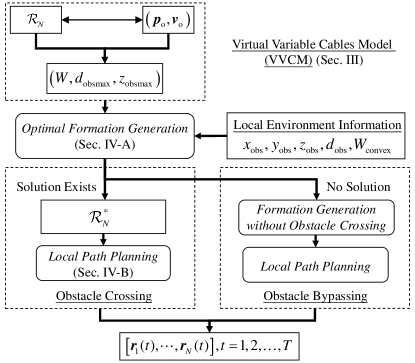
As discussed in Section III-B, the robot team has multiple possible formations due to combination of various taut/slack virtual cables and variable angle . We formulate a constrained nonlinear optimization to compute an optimal robot formation. For obstacle avoidance in 3D space, passing from the top of obstacles (i.e., obstacle crossing) is preferred than passing from aside of obstacles. If no feasible formation is found for obstacle crossing, the planner then finds paths that bypass obstacles as demonstrated in [21]. Fig. 4 illustrates the overall design of the motion planner.
The robot formation can be characterized by , . The optimization problem considers to use formation variables to minimize cost that is given by
| (11) |
where , , and are costs to penalize transportation, passable area and obstacle crossing, respectively. ensures the safety and stability of system during transportation. In order to ensure that each robot participates in the handling of the object, each virtual cable is taut and is given by
| (12) |
where and are initial positions of the object in and the th robot’s planar position, respectively, , and are the weighting factors. Cost keeps the robot team in a safe range and ensures that the formation can rotate freely during obstacle avoidance. Therefore, is designed as
| (13) |
where penalizes the outline size of the robot team. Cost ensures that the formation can cross the obstacle in any direction and keeps the object at a safe height,
| (14) |
where weights penalize the height of object crossing the obstacle and robotic formation size, respectively.
From the above discussion, it is clear that hinders the deformation of the robot team, limits the size of the formation, while is the key item to ensure the obstacle crossing. With these cost functions, the optimization problem is formulated as
| (15a) | ||||
| subject to | (15b) | |||
| (15c) | ||||
where the indicators and of the robotic formation should be larger than the and of the local obstacle. Constraint (15c) enforces that the robot formation configuration variables defined in Section II-A are within their corresponding limits.
IV-B Local Motion Planning
With the optimized robot formation , we still need to specify their trajectory to pass through one obstacle at a time. We keep the robot formation and try to rotate the entire formation shape to find a trajectory for crossing or bypassing obstacles.
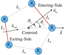
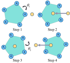
Fig. 5 illustrates the robot path generation design for a five-robot team. As shown in Fig. 5, each side of the robot formation is denoted as . We consider the forward velocity direction of the formation centroid as the -axis. By the definition of in (2), the robot formation can pass from the top of the obstacle from any and the normal vectors for the obstacle to enter or exit the formation are denoted as and , respectively. There are four steps for obstacle crossing, as shown in Fig. 5. In the first step, , the robot formation rotates about its centroid for angle such that coincides with the -axis. The formation then translates to cross the obstacle from time moments to . In the third step, , the formation rotates with angle and vector aligns with the -axis, where is the relative angle between and ; see Fig. 5. Finally, the formation travels to pass from the top of the obstacle at time . During the entire process, the translational speed of the robot formation is assumed to be constant, and the time instances , , are determined by the moving distance.
We denote the robot formation centroid path as . From the above discussion, we have and a path generation is then designed as
where . and are determined according to different entering and exiting side, which are positive in the counterclockwise direction. Algorithm 2 summarizes the path generation design for the robot team. Compared with the existing obstacle bypassing paths, the path generated by Algorithm 2 is to let the transported object cross over the obstacle.
V Experimental Results
In this section, we demonstrate the planning algorithms by experiments and simulation. A three-robot team is used as an experimental platform and simulation demonstrates the motion planning algorithms for more than three robots case.
V-A Experimental Setup
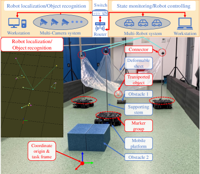
Fig. 6 shows the experimental setup and communication network of the system. Three robots (Turtlebot3 Waffle-Pi) were used in experiment. The transported object was a billiard ball. The position of the robots and the object were acquired by a motion capture system (8 cameras from NOKOV) at a rate of Hz. Plastic cloth sheets were used in experiments. Each side length of the sheet was m and the height of each holding point was m. The experimental environment was a corridor (2 meters wide, 6 meters long) with two different-height obstacles in the middle. The first obstacle (Obstacle #1) was a circular shape with a radius of m and a height of cm, and the other (Obstacle #2) had a radius of m and a height of m. The robot controller was implemented in robot operating system (ROS) with embedded system (NVIDIA Jetson NANO and OpenCR controller). A remote laptop (Intel i7-4710HQ CPU with four cores and 8 GB RAM) was set up for state monitoring and robot controlling. The following model parameters were used in experiments: , , , , , cm, and cm.
V-B Experimental Results
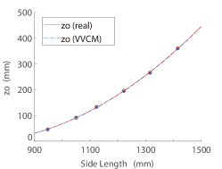
We first show the effectiveness of the VVCM and Algorithm 1. The accuracy of the object height is the key to verifying the validity of the model. The first experiment was conducted with the equilateral triangle formation as an example to verify the model. The actual heights of the object under different equilateral triangle formations were measured and compared with the VVCM. Fig. 7(a) shows the validation of the object height prediction by the VVCM. The root mean squared error (RMSE) of the height prediction by the VVCM is mm, and the error in the plane is mm. The model prediction error might mainly come from the positioning measurement variation of the billiard ball. The results confirm that the VVCM prediction is consistent with the experiments under different formation variations. Figs. 7(b)-(d) show the VVCM calculation examples of direct kinematics under different combinations of taut/slack status of virtual cables in a five-robot team. These results confirm that the position of the object can be obtained by the VVCM for any feasible formation.
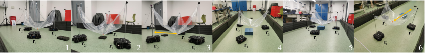
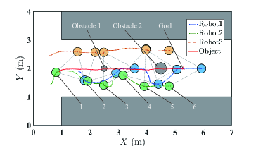
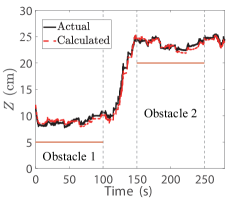
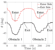
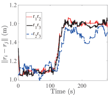
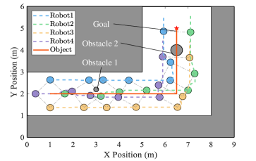
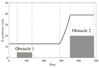
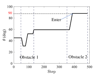
Due to the narrow corridor environment with obstacles in experiments, the motion planner such as that in [21] cannot obtain the feasible trajectory successfully because it only considers the obstacle bypassing in 2D space. The proposed motion planner instead generated the feasible obstacle-crossing trajectory successfully. Fig. 8 shows the snapshots of the robot formation and trajectory and Fig. 9 shows the detailed trajectories of the robot motion. The object went straight crossing over the two obstacles and the RMSE in the plane is mm. For crossing Obstacle #1, the average side lengths of the robot formation were , and m (exiting side). For crossing Obstacle #2, the average side lengths of the formation were , and m (exiting side). Fig. 9 shows the comparison results of the height of the object in experiments and the VVCM prediction. The RMSE of the VVCM prediction is mm. The average heights of the object in the process of crossing Obstacles #1 and #2 were respectively cm and cm, which were both safe. Fig. 9 shows the angles of the normal vectors at the entering and exiting sides. The entering angles for the robot formation to cross two obstacles were and , respectively, and the exiting angles were both , which was consistent with the local path generation method discussed in Section III-B. Fig. 9 shows the relative distances among the robots. It is clear that the relative distance changes corresponded to the object’s height changes as shown in Fig. 9. The main source of the fluctuation in these figures was from the robot speed variations due to the nonholonomic nature of the used robots when the formation rotated.
We further run simulation studies with - and -robot teams in different scenarios to verify the scalability of the motion planner. Fig. 10 shows the results for a -robot team to pass a turned corridor while carrying the object. Fig. 10 shows the robot motion trajectories, Fig. 10 shows the object height trajectory during transporting and Fig. 10 demonstrates the entering angle profiles of the robot formation when crossing obstacle. In this example, different exiting edges of the robot formation were selected and when there is no need to rotate, the formation can pass the obstacle from the top directly. The robot formation successfully followed the center-line of the trajectory, while rotating was used to pass crossing two obstacles. Indeed, the planner can be widely used to various numbers of robots and the algorithm is scalable. To apply this planner to complex environments, the robots should be equipped with diverse sensors to detect obstacles and build the map in real time. Distributed sensing and real-time control algorithms are required in these applications. Due to page limit, we demonstrate the detailed results of a -robot team in the companion video clip.
VI Conclusion
We proposed to use the virtual variable cables model to capture motion of the object in the deformable sheet that was collaboratively held by a multi-robot transporting system. Based on the VVCM, a motion planner was then proposed for transporting the object by the multi-robot. One attractive feature of the motion planner was its capability for crossing obstacles in 3D space. Compared with existing collaborative multi-robot object transporting approaches, the proposed planner gave priority to crossing obstacles instead of bypassing obstacles. This property improved the efficiency to traverse through cluttered environments (e.g., narrow corridors with obstacles) in which the traditional methods cannot achieve. The experiments and simulation were also presented to validate the VVCM and demonstrate the planning algorithms.
References
- [1] B. Roy, A. Basnajian, and H. H. Asada, “Repositioning of a rigid body with a flexible sheet and its application to an automated rehabilitation bed,” IEEE Trans. Automat. Sci. Eng., vol. 2, no. 3, pp. 300–307, 2005.
- [2] E. Tuci, M. H. Alkilabi, and O. Akanyeti, “Cooperative object transport in multi-robot systems: A review of the state-of-the-art,” Front. Robot. AI, vol. 5, 2018, article 59.
- [3] Z. Wang and M. Schwager, “Force-amplifying n-robot transport system (force-ants) for cooperative planar manipulation without communication,” Int. J. Robot. Res., vol. 35, no. 13, pp. 1564–1586, 2016.
- [4] Y. Ren, S. Sosnowski, and S. Hirche, “Fully distributed cooperation for networked uncertain mobile manipulators,” IEEE Trans. Robotics, vol. 36, no. 4, pp. 984–1003, 2020.
- [5] R. Herguedas, G. López-Nicolás, R. Aragüés, and C. Sagüés, “Survey on multi-robot manipulation of deformable objects,” in Proc. 2019 IEEE Int. Conf. Emerg. Technol. Factory Automat., 2019, pp. 977–984.
- [6] F. Nadon, A. J. Valencia, and P. Payeur, “Multi-modal sensing and robotic manipulation of non-rigid objects: A survey,” Robotics, vol. 7, no. 4, p. 74, 2018.
- [7] X. Provot et al., “Deformation constraints in a mass-spring model to describe rigid cloth behaviour,” in Prof. Graph. Interf., Quebec, Canada, 1995, pp. 147–147.
- [8] J. Weil, “The synthesis of cloth objects,” ACM Trans. Graph., vol. 20, no. 4, pp. 49–54, 1986.
- [9] Y. Bai, W. Yu, and C. K. Liu, “Dexterous manipulation of cloth,” in Computer Graphics Forum, vol. 35, no. 2. Wiley Online Library, 2016, pp. 523–532.
- [10] J. Alonso-Mora, R. Knepper, R. Siegwart, and D. Rus, “Local motion planning for collaborative multi-robot manipulation of deformable objects,” in Proc. IEEE Int. Conf. Robot. Autom., Seattle, WA, 2015, pp. 5495–5502.
- [11] S. Chand, P. Verma, R. Tallamraju, and K. Karlapalem, “Transportation of deformable payload through static and dynamic obstacles using loosely coupled nonholonomic robots,” in Proc. 2019 Int. Symp. Multi-Robot Multi-Agent Syst., New Brunswick, NJ, 2019, pp. 228–230.
- [12] D. McConachie, A. Dobson, M. Ruan, and D. Berenson, “Manipulating deformable objects by interleaving prediction, planning, and control,” Int. J. Robot. Res., vol. 39, no. 8, pp. 957–982, 2020.
- [13] K. Hunte and J. Yi, “Collaborative object manipulation through indirect control of a deformable sheet by a mobile robotic team,” in Proc. IEEE Conf. Automat. Sci. Eng., Vancouver, Canada, 2019, pp. 1463–1468.
- [14] ——, “Collaborative manipulation of spherical-shape objects with a deformable sheet held by a mobile robotic team,” in Proc. Model., Est. Control Conf., Austin, TX, 2021, pp. 437–442.
- [15] ——, “Pose control of a spherical object held by deformable sheet with multiple robots ,” in Proc. Model., Est. Control Conf., Jersey City, NJ, 2022.
- [16] A. Capua, A. Shapiro, and S. Shoval, “Motion analysis of an underconstrained cable suspended mobile robot,” in Proc. IEEE Int. Conf. Robot. Biomimet., Guilin, China, 2009, pp. 788–793.
- [17] ——, “Motion planning algorithm for a mobile robot suspended by seven cables,” in Proc. 2010 IEEE Conf. Robot., Automat. Mechatron., Singapore, 2010, pp. 504–509.
- [18] ——, “Spiderbot: a cable suspended mobile robot,” in Proc. IEEE Int. Conf. Robot. Autom., Shanghai, China, 2011, pp. 3437–3438.
- [19] J. Hu, J. Sun, Z. Zou, D. Ji, and Z. Xiong, “Distributed multi-robot formation control under dynamic obstacle interference,” in Proc. IEEE/ASME Int. Conf. Adv. Intelli. Mechatronics, Boston, MA, 2020, pp. 1435–1440.
- [20] X. Zhang, L. Yan, T. L. Lam, and S. Vijayakumar, “Task-space decomposed motion planning framework for multi-robot loco-manipulation,” in Proc. IEEE Int. Conf. Robot. Autom., Xi’an, China, 2021, pp. 8158–8164.
- [21] J. Alonso-Mora, S. Baker, and D. Rus, “Multi-robot formation control and object transport in dynamic environments via constrained optimization,” Int. J. Robot. Res., vol. 36, no. 9, pp. 1000–1021, 2017.