Optimal consumption and portfolio selection with Epstein-Zin utility under general constraints

Abstract

The paper investigates the consumption-investment problem for an investor with Epstein-Zin utility in an incomplete market. Closed, not necessarily convex, constraints are imposed on strategies. The optimal consumption and investment strategies are characterized via a quadratic backward stochastic differential equation (BSDE). Due to the stochastic market environment, solutions to this BSDE are unbounded and thereby the BMO argument breaks down. After establishing the martingale optimality criterion, by delicately selecting Lyapunov functions, the verification theorem is ultimately obtained. Besides, several examples and numerical simulations for the optimal strategies are provided and illustrated.

1 Introduction

In the classical representative agent framework, the investor’s preferences are mostly characterized by time-separable utility functions. Optimal consumption-investment problem for this kind of utility has been developed comprehensively by numerous researchers. Originally articulated in the context of the Markovian structure in the landmark paper by Merton (1971), the theory was later extended to non-Markovian models by Pliska (1986), Karatzas, Lehoczky and Shreve (1987) and Cox and Huang (1989) using the martingale method in a complete market. Kramkov and Schachermayer (1999) gave a duality result and Hu, Imkeller and Müller (2005) investigated the problem by the method of backward stochastic differential equations (BSDEs) for a class of time separable utilities in an incomplete market. See Pham (2008) for more related problems with time separable utilities.

However, widely used time separable utilities unintentionally impose an artificial relation between risk aversion $\gamma$ and elasticity of intertemporal substitution (EIS) $\psi$: they are reciprocal to each other. Such a relationship will lead to a large number of asset pricing anomalies, such as the low risk premium and high risk-free rate. To disentangle risk aversion from EIS, the notion of recursive utilities was first specified in discrete time by Epstein and Zin (1989). Then its continuous-time analog was formulated in Duffie and Epstein (1992). These Epstein-Zin type utilities provide a framework to tackle the aforementioned asset puzzles. The readers can refer to Bansal (2007); Bansal and Yaron (2004); Benzoni, Collin-Dufresne and Goldstein (2011) for more explanations and clarifications on $\gamma$ and $\psi$.

Over the past two decades, there has been substantial progress for the consumption and investment problem with recursive utility of Epstein-Zin type in stochastic market environments. Using the utility gradient approach, Schroder and Skiadas (1999) studied the optimal strategies for Epstein-Zin utility with parameter $\theta=\frac{1-\gamma}{1-1/\psi}<0$. Kraft, Seifried and Steffensen (2013) and Kraft, Seiferling and Seifried (2017) investigated the problem for Epstein-Zin utility with assumption (H) on parameters excluding $\gamma>1$ and $\psi>1$ by the tool of Hamilton-Jacobi-Bellman (HJB) equations. Motivated by empirical evidences and observations suggesting the parameters $\gamma>1$ and $\psi>1$, Xing (2017) considered the corresponding problem for Epstein-Zin utility with the advantage of BSDE techniques. Besides, Matoussi and Xing (2018) introduced a dual approach to study the consumption-investment problem for Epstein-Zin utility with parameters $\gamma\psi>1$ and $\psi>1$.

In the vast majority of the literature, it is often assumed that the investor is able to select his consumption and portfolio strategies with some constraints. For time-additive utilities, Cvitanic and Karatzas (1992) studied the stochastic control problem of maximizing expected utility from terminal wealth when the portfolio is constrained to take values in a closed convex set. One can refer to Rouge and El Karoui (2000) and Bian, Chen and Xu (2019) for more information about convex trading constraints. More importantly, Hu, Imkeller and Müller (2005) solved the optimal investment problem with closed but not necessarily convex set constraints for time-additive utilities, such as exponential utility or constant relative risk aversion (CRRA) utility. Later, Cheridito and Hu (2011) introduced closed constraints for the consumption process based on the work of Hu, Imkeller and Müller (2005).

For recursive utilities, El Karoui, Peng and Quenez (2001) stated a dynamic maximum principle to examine the consumption-investment problem with recursive utilities in the presence of nonlinear constraints on the wealth. Schroder and Skiadas (2003, 2005) considered convex constraints on strategies. Wang, Wang and Yang Wang, Wang and Yang (2016) developed a tractable incomplete market model with an earning process subject to permanent shocks and borrowing constraints. The readers can also refer to Aurand and Huang (2021) and Melnyk, Muhle-Karbe and Seifried (2020) for maximizing Epstein-Zin utility with random horizons and transaction costs respectively.

Motivated by Hu, Imkeller and Müller (2005) and Cheridito and Hu (2011), the current paper is committed to studying the optimal consumption and investment problem for Epstein-Zin utility with closed constraints on strategies in an incomplete market whose parameters are driven by a state variable. Using the same framework as in Xing (2017), we focus on the specification $\gamma>1$ and $\psi>1$. Compared to existing results, this paper contributes to the literature in the following three aspects.

First, we impose the constraints on strategies for Epstein-Zin utility, which is supposed to simply be closed. To our best knowledge, this general constraints have not been investigated for Epstein-Zin utility before. Due to closed constraints on strategies, the utility gradient approach and the dual method are no longer available. Our method is based on BSDE techniques coming from Hu, Imkeller and Müller (2005) and Xing (2017). Comparing with Xing (2017), the BSDE derived by the martingale optimal principle is more complicated, which is involved a projection term on a closed set. Fortunately, this term does not essentially change the quadratic structure of the BSDE. However, the distance function not only contains term $z$, but also involves the unbounded market parameters. This fact presents difficulties in proving the properties of BSDE’s solutions. After careful estimations, the upper boundedness of the solution still holds under appropriate assumptions. It deserves pointing out that we present the martingale optimal principle (Theorem 3.1) as one of our main results, which is implicit in Xing (2017).

Second, our model admits market parameters unbounded. Solutions to this quadratic BSDE are unbounded and thereby the often-used BMO argument breaks down. Closed constraints on the set of admissible strategies result in a situation that the candidate optimal strategy cannot be explicitly expressed by $Z$, one part of solutions to the BSDE. To prove this exponential local martingale (induced by the stochastic integral term of the optimal strategy) is a martingale, we need to carry out more sophisticated estimations and choose delicately a suitable Lyapunov function to overcome the difficulties. Unlike the situation of Xing (2017), we find the effect of constraints on portfolio causes the Lyapunov argument may fail for sufficiently large $\gamma$. We propose the condition $\frac{1}{2}+\frac{2(1-\gamma)}{\gamma}\left|\sigma^{\prime}\Sigma^{-1}\sigma\rho\right|\left|\rho\right|>0$ to proceed the argument, and illustrate the universality of the method. Consequently, the verification theorem holds.

Third, we provide three specific numerical examples to illustrate the influence of the constraints and comparative statics analysis on the optimal strategy. The first one is Black-Scholes model. As far as we know, Epstein-Zin utility model with closed constraints has not been investigated before even in this simplest market model. We change the portfolio constraints to show its impact on the portfolio and consumption. Linear diffusion model and Heston stochastic volatility model are also investigated. The former model corresponds to a bounded risk premium and volatility, while in the latter case both risk premium and volatility are unbounded. We find the constraints have a smaller impact on consumption, but a larger impact on investment portfolios.

The remainder of this paper is organized as follows. Section 2 introduces the Epstein-Zin utility process. Section 3 presents the stochastic market environment, the consumption-investment problem and main results including the martingale optimal principle and the verification theorem. Several examples and numerical simulations for the optimal strategies are provided and illustrated in Section 4. All the proofs are relegated to Section 5. Section 6 concludes the paper.

2 Epstein-Zin preferences

Given a time horizon $T<+\infty$. Let $\left(\Omega,\mathscr{F},\left(\mathscr{F}_{t}\right)_{0\leq t\leq T},\mathbb{P}\right)$ be a filtered probability space. $\left(\mathscr{F}_{t}\right)_{0\leq t\leq T}$ is the natural filtration generated by a $(k+n)$-dimensional standard Brownian motion $B=\left(W,W^{\perp}\right)$, where $W$ and $W^{\perp}$ are the first $k$ and the last $n$ components. We also assume $\left(\mathscr{F}_{t}\right)_{0\leq t\leq T}$ satisfies the usual hypotheses, completeness and right-continuity.

Let $\mathcal{R}_{+}$ be the set of all nonnegative progressively measurable processes on $[0,T]$. For $c\in\mathcal{R}_{+}$, if $t<T$, $c_{t}$ represents the consumption rate at time $t$; $c_{T}$ stands for a lump sum consumption at $T$. Throughout the whole paper, we always assume $\delta>0,\gamma>1$ and $\psi>1$, which stand for the discounting rate, the relative risk aversion and the EIS respectively. Given the bequest utility function $U(c)=\frac{c^{1-\gamma}}{1-\gamma}$, the Epstein-Zin utility for the consumption stream $c\in\mathcal{R}_{+}$ over a time horizon $T$ is a semimartingale $V^{c}$ that satisfies

$$V_{t}^{c}=\mathbf{E}_{t}\left[\int_{t}^{T}f(c_{s},V_{s}^{c})ds+U(c_{T})\right],~{}~{}~{}\forall t\in[0,T],$$ (1)

where $\mathbf{E}_{t}(\cdot)$ denotes $\mathbf{E}(\cdot|\mathscr{F}_{t})$ throughout the paper and $f:[0,+\infty)\times(-\infty,0]\to\mathbb{R}$ stands for the Epstein-Zin aggregator denoted by

$$f(c,v) =\delta\frac{(1-\gamma)v}{1-\frac{1}{\psi}}\left[\left(\frac{c}{((1-\gamma)v)^{\frac{1}{1-\gamma}}}\right)^{1-\frac{1}{\psi}}-1\right]$$

$$=\frac{\delta c^{1-\frac{1}{\psi}}}{1-\frac{1}{\psi}}\left((1-\gamma)v\right)^{1-\frac{1}{\theta}}-\delta\theta v,$$ (2)

where

$$\theta:=\frac{1-\gamma}{1-\frac{1}{\psi}}<0.$$

By Proposition 2.2 in Xing (2017), $V^{c}$ can be characterized by the following BSDE

$$V_{t}^{c}=U(c_{T})+\int_{t}^{T}f(c_{s},V_{s}^{c})ds-\int_{t}^{T}Z_{s}^{c}dB_{s},~{}~{}~{}t\in[0,T].$$ (3)

Specifically, let $\mathcal{C}_{a}$ denote the class of consumption streams

$$\mathcal{C}_{a}:=\left\{c\in\mathcal{R}_{+}:\mathbf{E}\left[\int_{0}^{T}e^{-\delta s}c_{s}^{1-\frac{1}{\psi}}ds\right]<+\infty,\mathbf{E}\left[c_{T}^{1-\gamma}\right]<+\infty\right\}.$$

Then for each $c\in\mathcal{C}_{a}$, BSDE (3) admits a unique solution $(V^{c},Z^{c})$ in which $V^{c}$ is continuous, strictly negative, of class D, and $\int_{0}^{T}|Z_{t}^{c}|^{2}dt<+\infty$, a.s.

Remark 2.1.

It is worth noting that BSDE (3) only requires the integrable terminal condition. The readers can refer to Theorem 1 of Fan (2018) for general results.

Remark 2.2.

Among the literature on Epstein-Zin utility, there exists another kind of integrability requirement on consumption streams

$$\mathbf{E}\left[\int_{0}^{T}c_{t}^{l}dt+c_{T}^{l}\right]<+\infty,\quad\forall l\in\mathbb{R}.$$

One can refer to Schroder and Skiadas (1999, 2003, 2005), Kraft, Seifried and Steffensen (2013) and Kraft, Seiferling and Seifried (2017). However, these conditions are not general enough to capture all relevant consumption plans in our applications. $\mathcal{C}_{a}$ is the same as the one considered in Xing (2017), which is weaker than aforementioned conditions.

3 The consumption-investment problem

Motivated by Hu, Imkeller and Müller (2005), Cheridito and Hu (2011) and Xing (2017), we will investigate the consumption-investment optimization with Epstein-Zin utility under general constraints in an incomplete market. Following the financial market framework of Xing (2017), we introduce closed constraints on consumption and investment strategies, and derive the martingale optimal principle (Theorem 3.1), from which the candidate optimal strategy can be deduced. Under some mild restrictions on market parameters, the verification theorem (Theorem 3.2) is given by the Lyapunov function argument.

3.1 The model setup

Let $E$ be an open domain in $\mathbb{R}^{k}$, and define an $E$-valued state process

$$dX_{t}=b(t,X_{t})dt+a(t,X_{t})dW_{t},\quad X_{0}=x\in E,$$ (4)

where $b,a:\mathbb{R}_{+}\times E\to\mathbb{R}^{k}$ are given Borel measurable functions. Consider a financial market model consisting of a riskfree asset $S^{0}$ and risky assets $S=(S^{1},\cdots,S^{n})$, which satisfy the dynamics

$$dS_{t}^{0}=r(t,X_{t})S_{t}^{0}dt,$$

$$dS_{t}=\operatorname{diag}(S_{t})\left[\left(r(t,X_{t})\mathbf{1}_{n}+\mu(t,X_{t})\right)dt+\sigma(t,X_{t})dW_{t}^{\rho}\right],$$

where diag($S$) is a diagonal matrix with the elements of $S$ on the diagonal. Here $\mathbf{1}_{n}$ is an $n$-dimensional vector with each entry 1. $W^{\rho}:=\int_{0}^{\cdot}\rho(s,X_{s})dW_{s}+\int_{0}^{\cdot}\rho^{\perp}(s,X_{s})dW^{\perp}_{s}$ is an $n$-dimensional Brownian motion with correlation functions $\rho:\mathbb{R}_{+}\times E\to\mathbb{R}^{n\times k}$ and $\rho^{\perp}:\mathbb{R}_{+}\times E\to\mathbb{R}^{n\times n}$ satisfying $\rho\rho^{\prime}+\rho^{\perp}\left(\rho^{\perp}\right)^{\prime}=I_{n}$. Model coefficients $r:\mathbb{R}_{+}\times E\to\mathbb{R},\mu:\mathbb{R}_{+}\times E\to\mathbb{R}^{n},\sigma:\mathbb{R}_{+}\times E\to\mathbb{R}^{n\times n}$ are all given Borel measurable functions.

Let $\mathcal{R}^{n}_{+}$ be the set of all predictable processes taking their values in $\mathbb{R}^{n}$. We allow constraints both on the investment strategy $\pi$ and the consumption process $c$. To this end, we introduce nonempty subsets $\Lambda\subseteq\mathcal{R}^{n}_{+}$ and $\mathcal{C}\subseteq\mathcal{C}_{a}$. Then we use the following concepts from Definition 3.1 and Definition 2.1 of Cheridito, Kupper and Vogelpoth (2015): $\Lambda$ (resp. $\mathcal{C}$) is sequentially closed if it contains each process $\pi$ (resp. $c$) that is the $\lambda\otimes\mathbb{P}\raisebox{0.0pt}{-}a.s.$ limit of a sequence $(\pi^{n})_{n\geq 1}$ (resp. $(c^{n})_{n\geq 1}$) of processes in $\Lambda$ (resp. $\mathcal{C}$). $\Lambda$ (resp. $\mathcal{C}$) is $\mathcal{R}_{+}$-stable if it contains $1_{B}a+1_{B^{c}}a^{\prime}$ for all $a,a^{\prime}\in\Lambda$ (resp. $a,a^{\prime}\in\mathcal{C}$) and each predictable set $B\subseteq[0,T]\times\Omega$. See more details in Cheridito and Hu (2011).

Suppose that $\Lambda$ and $\mathcal{C}$ satisfy the following assumption.

Assumption 3.1.

$\Lambda$ and $\mathcal{C}$ are sequentially closed and $\mathcal{R}_{+}$-stable.

It follows from Cheridito and Hu (2011) that $\mathcal{A}:=\{\sigma^{\prime}\pi:\pi\in\Lambda\}$ is sequentially closed and $\mathcal{R}_{+}$-stable subset of $\mathcal{R}^{n}_{+}$. Writing $p_{t}=\sigma^{\prime}_{t}\pi_{t}$, we also call such $p$ the investment strategy.

For an predictable process $u$ in $\mathbb{R}^{n}_{+}$, the distance between $u$ and $\mathcal{A}$ is a predictable process defined as

$$\operatorname{dist}\left(\mathcal{A},u\right):=\operatorname{essinf}_{p\in\mathcal{A}}|u-p|.$$

The set $\Pi\left(\mathcal{A},u\right)$ consists of those elements in $\mathcal{A}$ at which the greatest lower bound with respect to the $\lambda\otimes\mathbb{P}\raisebox{0.0pt}{-}a.s.$ order is obtained

$$\Pi\left(\mathcal{A},u\right):=\left\{p\in\mathcal{A}:|u-p|=\operatorname{dist}\left(\mathcal{A},u\right)\right\}.$$

It is shown in Corollary 4.5 of Cheridito, Kupper and Vogelpoth (2015) that $\Pi\left(\mathcal{A},u\right)$ is nonempty.

We enforce the following conditions on market coefficients.

Assumption 3.2.

Each of $b,a,r,\mu,\sigma,\rho,\rho^{\perp}$ is continuous in $t$ and local Lipschitz-continuous in domain $E$. $A:=aa^{\prime}$ and $\Sigma:=\sigma\sigma^{\prime}$ are both positive definite. $r\geq r_{\operatorname{min}}$ and $0<\mu^{\prime}\Sigma^{-1}\mu\leq C_{0}$, where $r_{\operatorname{min}}$ and $C_{0}$ are two constants. Without loss of generality, suppose $r_{min}<0$.

Note that we work in a financial environment with a bounded from below interest rate $r$ and a bounded square of market risk price $\mu^{\prime}\Sigma^{-1}\mu$, where both the risk premium $\mu$ and volatility $\sigma$ can be unbounded. Since $r$ is bounded from below, so is $r+\frac{1}{2\gamma}\mu^{\prime}\Sigma^{-1}\mu$.

An agent must choose a consumption process $c$ and an investment strategy $p$ to invest in this financial market. Given an initial wealth $\omega$, the corresponding wealth process $\mathcal{W}^{c,p}$ is given by

$$d\mathcal{W}_{t}^{c,p}=\mathcal{W}_{t}^{c,p}\left(\left(r_{t}+p_{t}^{\prime}\sigma_{t}^{\prime}\Sigma_{t}^{-1}\mu_{t}\right)dt+p_{t}^{\prime}dW_{t}^{\rho}\right)-c_{t}dt,\quad\mathcal{W}_{0}^{c,p}=\omega,$$

where $r_{t},\sigma_{t},\mu_{t},\rho_{t}$ represents $r(t,X_{t}),\sigma(t,X_{t}),\mu(t,X_{t}),\rho(t,X_{t})$ respectively. A strategy $(c,p)$ is called admissible if it belongs to

$$\mathcal{S}_{a}=\left\{(c,p):c\in\mathcal{C},p\in\mathcal{A}\ {\rm and}\ \left(\mathcal{W}^{c,p}\right)^{1-\gamma}e^{Y}{\rm\ is\ of\ class\ D}\right\},$$ (5)

where $Y$ is one solution to BSDE (9).

The agent wants to solve the maximization problem

$$V_{0}:=\sup_{(c,p)\in\mathcal{S}_{a}}V_{0}^{c,p}=\sup_{(c,p)\in\mathcal{S}_{a}}\mathbf{E}\left[\int_{0}^{T}f(c_{s},V_{s}^{c})ds+U(\mathcal{W}^{c,p}_{T})\right].$$ (6)

3.2 The martingale optimal principle

For convenience, we do not put closed constraints on consumption process $c$ in Subsection 3.2 and 3.3. See Remark 3.5 for corresponding results about $c$. In this case, the set of admissible strategies $\mathcal{S}_{a}$ has the following form

$$\mathcal{S}_{a}=\left\{(c,p):c\in\mathcal{C}_{a},p\in\mathcal{A}\ {\rm and}\ \left(\mathcal{W}^{c,p}\right)^{1-\gamma}e^{Y}{\rm\ is\ of\ class\ D}\right\}.$$

We make the following assumption for investment strategies:

$${\rm there\ exists\ a\ bounded\ process\ }\underline{p}\ {\rm in}\ \mathcal{A}\ {\rm such\ that}\ |\underline{p}|\leq C_{p}\ {\rm where}\ C_{p}\ {\rm is\ a\ constant}.$$ (7)

In the following we suppress the supscript $(c,p)$ of $\mathcal{W}^{c,p}$. By the martingale optimal principle, we construct a so-called utility process

$$G_{t}^{c,p}:=\frac{\mathcal{W}_{t}^{1-\gamma}}{1-\gamma}e^{Y_{t}}+\int_{0}^{t}f\left(c_{s},\frac{\mathcal{W}_{s}^{1-\gamma}}{1-\gamma}e^{Y_{s}}\right)ds,\quad t\in[0,T],$$ (8)

where

$$Y_{t}=\int_{t}^{T}H(s,Y_{s},Z_{s})ds-\int_{t}^{T}Z_{s}dW_{s},\quad t\in[0,T],$$ (9)

with

$$H(t,y,z)= -\frac{\gamma(1-\gamma)}{2}\operatorname{dist}^{2}\left(\mathcal{A}_{t},\frac{1}{\gamma}\sigma_{t}^{\prime}\Sigma_{t}^{-1}(\mu_{t}+\sigma_{t}\rho_{t}z^{\prime})\right)+z\left(\frac{1}{2}I_{k}+\frac{1-\gamma}{2\gamma}\rho_{t}^{\prime}\sigma_{t}^{\prime}\Sigma_{t}^{-1}\sigma_{t}\rho_{t}\right)z^{\prime}$$ (10)

$$+\frac{1-\gamma}{\gamma}\mu_{t}^{\prime}\Sigma_{t}^{-1}\sigma_{t}\rho_{t}z^{\prime}+\frac{\theta}{\psi}\delta^{\psi}e^{-\frac{\psi}{\theta}y}+\frac{1-\gamma}{2\gamma}\mu_{t}^{\prime}\Sigma_{t}^{-1}\mu_{t}+(1-\gamma)r_{t}-\delta\theta.$$

In fact, $H$ is chosen such that $G$ is a local martingale for candidate optimal strategy. Comparing with Xing (2017), BSDE (9) derived by the martingale optimal principle is more complicated, which is involved a projection term on a closed set. Fortunately, this term does not essentially change the quadratic structure of the BSDE. Similar to Xing (2017), the upper boundedness for the solution still holds under the parameter specification $\gamma>1$ and $\psi>1$. For the convenience of the proof, we add the following Assumption 3.3, making us to deal with the linear term of $z$ by Girsanov transformation and to derive the estimations of $Y$.

Assumption 3.3.

$$\frac{d\hat{\mathbb{P}}}{d\mathbb{P}}=\mathscr{E}\left(\int\frac{1-\gamma}{\gamma}\mu^{\prime}\Sigma^{-1}\sigma\rho dW_{s}\right)_{T}$$

defines a new probability measure $\hat{\mathbb{P}}$ equivalent to $\mathbb{P}$. In addition (throughout the paper, $\hat{\mathbf{E}}(\cdot)$ denotes the expectation with respect to $\hat{\mathbb{P}}$), $\hat{\mathbf{E}}\left[\int_{0}^{T}r_{s}ds\right]<+\infty.$

The following proposition shows that $Y$ is bounded from above, which is very important for our subsequent proofs.

Proposition 3.1.

Let $\gamma,\psi>1$ and Assumptions 3.1, 3.2 and 3.3 hold. Then BSDE (9) has at least one solution $(Y,Z)$ such that

$$(1-\gamma)\hat{\mathbf{E}}_{t}\left[\int_{t}^{T}r_{s}ds\right]+C_{2}(t)\leq Y_{t}\leq C_{1}T,\quad\forall t\in[0,T],$$ (11)

and $\hat{\mathbf{E}}\left(\int_{0}^{T}|Z_{s}|^{2}ds\right)<+\infty$, where

$$C_{1}:=(1-\gamma)r_{min}-\delta\theta+2(C_{0}+\gamma(\gamma-1)C_{p}),$$

$$C_{2}(t):=\left[\frac{\theta}{\psi}\delta^{\psi}\operatorname{exp}\left(-\frac{\psi}{\theta}C_{1}T\right)+\frac{1-\gamma}{2\gamma}C_{0}-\delta\theta\right](T-t).$$

Now we are ready to declare the main theorem in this subsection. Before that write $\mathcal{W}^{c^{*},p^{*}}$ briefly as $\mathcal{W}^{*}$, where $c^{*}$ and $p^{*}$ are given by (12).

Theorem 3.1.

(Martingale optimal principle) Let Assumptions 3.1, 3.2 and 3.3 hold. Suppose $(Y,Z)$ is a solution to BSDE (9). Then

1. For any $(c,p)\in\mathcal{S}_{a}$, $G^{c,p}$ is a local supermartingale and

   $$V_{t}^{c}\leq\frac{\mathcal{W}_{t}^{1-\gamma}}{1-\gamma}e^{Y_{t}},\quad\forall t\in[0,T].$$

2. Denote

   $$c^{*}=\hat{c}^{*}\mathcal{W}^{*}=\delta^{\psi}e^{-\frac{\psi}{\theta}Y}\mathcal{W}^{*},\quad p^{*}\in\Pi\left(\mathcal{A},\frac{1}{\gamma}\sigma^{\prime}\Sigma^{-1}(\mu+\sigma\rho Z^{\prime})\right),$$ (12)

   where $\mathcal{W}^{*}$ is the corresponding optimal wealth process. If $(c^{*},p^{*})\in\mathcal{S}_{a}$, then $G^{c^{*},p^{*}}$ is a local martingale and $(c^{*},p^{*})$ is the optimal strategy for problem (6). Moreover, for the initial wealth $\omega$, the optimal utility is given by

   $$V_{0}^{c^{*}}=\frac{\omega^{1-\gamma}}{1-\gamma}e^{Y_{0}}.$$

Remark 3.1.

The martingale optimal principle here is different from the one in Hu, Imkeller and Müller (2005). Thanks to the specific structure of Epstein-Zin utility, it is sufficient to obtain the optimality of utility and strategy that $G^{c,p}$ is a local supermartingale and $G^{c^{*},p^{*}}$ is a local martingale.

3.3 The verification theorem

In order to verify the martingale optimal principle, it is necessary to verify the stochastic exponential

$$M:=\mathscr{E}\left(\int(1-\gamma)(p^{*})^{\prime}dW^{\rho}+\int ZdW\right)$$ (13)

is a martingale under $\mathbb{P}$. We introduce an operator $\mathfrak{F}$ of a Lyapunov function $\phi$ to realize this goal. We borrowed this method from Chapter 10 of Stroock and Varadhan (2006) and Xing (2017). The readers can also refer to Robertson and Xing (2017) for more applications.

Assumption 3.4.

Suppose that $\frac{1}{2}+\frac{2(1-\gamma)}{\gamma}\left|\sigma^{\prime}\Sigma^{-1}\sigma\rho\right|\left|\rho\right|>0$ and $\phi\in C^{2}(E)$ is a Lyapunov function which satisfies following properties

1. $\lim_{n\to\infty}\inf_{x\in E\backslash E_{n}}\phi(x)=\infty$, where $(E_{n})$ is a sequence of open domains in $E$ satisfying $\cup_{n}E_{n}=E$, $\overline{E}_{n}$ compact and $\overline{E}_{n}\subseteq E_{n+1}$ for every $n$.

2. The operator

   $$\mathfrak{F}\left(\phi\right):= b^{\prime}\nabla\phi+\frac{1}{2}\sum_{i,j=1}^{k}A_{ij}\partial^{2}_{x_{i}x_{j}}\phi-\frac{2(1-\gamma)}{\gamma}\left|\sigma^{\prime}\Sigma^{-1}\mu\right|\left|\rho a^{\prime}\nabla\phi\right|-(1-\gamma)C_{p}\left|\rho a^{\prime}\nabla\phi\right|$$

   $$+\frac{1}{4}\frac{\left((1-\gamma)C_{p}|\rho|+\frac{2(1-\gamma)}{\gamma}\left|\sigma^{\prime}\Sigma^{-1}\mu\right|\left|\rho\right|-\left|\nabla\phi^{\prime}a\right|+\frac{2(1-\gamma)}{\gamma}\left|\sigma^{\prime}\Sigma^{-1}\sigma\rho\right|\left|\rho a^{\prime}\nabla\phi\right|\right)^{2}}{\frac{1}{2}+\frac{2(1-\gamma)}{\gamma}\left|\sigma^{\prime}\Sigma^{-1}\sigma\rho\right|\left|\rho\right|}$$ (14)

   is bounded from above on $E$.

Remark 3.2.

Our operator $\mathfrak{F}\left(\cdot\right)$ is much different from Xing (2017). Since we impose closed constraints on the set of admissible strategies, which causes the candidate optimal investment strategy (12) cannot be expressed by $Z$ explicitly. After subtle estimations and careful calculations, we delicately choose a suitable Lyapunov function to overcome the difficulties. In Section 4, we will give some examples and specific Lyapunov functions $\phi$ satisfying Assumption 3.4. Besides, the parameter condition $\frac{1}{2}+\frac{2(1-\gamma)}{\gamma}\left|\sigma^{\prime}\Sigma^{-1}\sigma\rho\right|\left|\rho\right|>0$ ensures ((ii)) is well-defined, and it always holds when $|\rho|$ is small enough.

Before giving the verification theorem, the following assumption ensures the integrability under a risk-neutral measure.

Assumption 3.5.

There exists a risk-neutral measure $\mathbb{P}_{0}$ denoted by

$$\frac{d\mathbb{P}_{0}}{d\mathbb{P}}=\mathscr{E}\left(\int-\lambda dW_{s}^{\rho}\right)_{T},$$

where $\lambda:\mathbb{R}_{+}\times E\to\mathbb{R}^{1\times n}$ is defined by $\mu^{\prime}=\lambda\sigma^{\prime}$. Furthermore,

$$\mathbf{E}^{0}\left[\operatorname{exp}\left((\psi-1)\int_{0}^{T}r_{s}^{+}ds\right)\mathscr{E}\left(\int\lambda_{s}dW_{s}^{0}\right)^{\psi}_{T}\right]<+\infty,$$

where $\mathbf{E}^{0}(\cdot)$ denotes the expectation under $\mathbb{P}_{0}$ and $W^{0}$ is a Brownian motion under $\mathbb{P}_{0}$.

Remark 3.3.

If $r$ and $\lambda$ are both bounded, the above assumption holds automatically. If $\sigma$ is symmetric, the risk-neutral measure $\mathbb{P}_{0}$ exists due to the boundedness of $\mu^{\prime}\Sigma^{-1}\mu$ from Assumption 3.2. The integrability condition in Assumption 3.5 can degenerate into a simpler one as follows: for sufficiently small $\epsilon>0$,

$$\mathbf{E}^{0}\left[\operatorname{exp}\left((1+\epsilon)(\psi-1)\int_{0}^{T}r_{s}^{+}ds\right)\right]<+\infty.$$

Then we can give our main result in this paper.

Theorem 3.2.

Let $\gamma$, $\psi>1$. Suppose Assumptions 3.1, 3.2, 3.3, 3.4 and 3.5 hold. Then $c^{*}$ and $p^{*}$ defined in (12) maximize the Epstein-Zin utility among all admissible strategies.

Corollary 3.1.

Suppose $\gamma$, $\psi>1$ and all market parameters are bounded. Then $c^{*}$ and $p^{*}$ defined in (12) maximize the Epstein-Zin utility among all admissible strategies. Moreover, for any initial wealth $\omega$, the optimal Epstein-Zin utility is given by

$$V_{0}^{c^{*}}=\frac{\omega^{1-\gamma}}{1-\gamma}e^{Y_{0}},$$

where $Y$ is one solution to BSDE (9).

Proof. When all market parameters are bounded, Assumptions 3.2, 3.3 and 3.5 hold obviously. Besides, Assumption 3.4 is not needed. Indeed, when all parameters are bounded, $Y$ is bounded, and the stochastic exponential $M$ can be proved to be a martingale by using the BMO argument directly.

Remark 3.4.

Corollary 3.1 provides an optimization result under bounded market parameters with Epstein-Zin type of recursive utilities. When $\gamma=\frac{1}{\psi}$, $V_{0}^{c}$ degenerates into time-separable utilities. One can refer to Hu, Imkeller and Müller (2005) and Cheridito and Hu (2011) for more details.

Remark 3.5.

Now we present results for the consumption process $c$ with closed constraints. We make a similar assumption on $\mathcal{C}$: there exists a bounded process $\underline{c}\in\mathcal{C}$. (When there is no constraints on $\mathcal{C}$, this condition is automatically satisfied since $0\in\mathcal{C}$.)

Recall that the admissible strategy is in (5) where

$$Y_{t}=\int_{t}^{T}H(s,Y_{s},Z_{s})ds-\int_{t}^{T}Z_{s}dW_{s},\quad t\in[0,T],$$

with

$$H(t,y,z)$$

$$= -\frac{\gamma(1-\gamma)}{2}\operatorname{dist}^{2}\left(\mathcal{A}_{t},\frac{1}{\gamma}\sigma_{t}^{\prime}\Sigma_{t}^{-1}(\mu_{t}+\sigma_{t}\rho_{t}z^{\prime})\right)+z\left(\frac{1}{2}I_{k}+\frac{1-\gamma}{2\gamma}\rho_{t}^{\prime}\sigma_{t}^{\prime}\Sigma_{t}^{-1}\sigma_{t}\rho_{t}\right)z^{\prime}$$

$$+\frac{1-\gamma}{\gamma}\mu_{t}^{\prime}\Sigma_{t}^{-1}\sigma_{t}\rho_{t}z^{\prime}+\inf_{\hat{c}\in\mathcal{C}}\left(-(1-\gamma)\hat{c}+\delta\theta e^{-\frac{1}{\theta}y}\hat{c}^{1-\frac{1}{\psi}}\right)+\frac{1-\gamma}{2\gamma}\mu_{t}^{\prime}\Sigma_{t}^{-1}\mu_{t}+(1-\gamma)r_{t}-\delta\theta.$$

Due to Assumption 3.1, we have the following estimation

$$\frac{\theta}{\psi}\delta^{\psi}e^{-\frac{\psi}{\theta}Y} =\inf_{\hat{c}\in\mathcal{R}_{+}}\left(-(1-\gamma)\hat{c}+\delta\theta e^{-\frac{1}{\theta}Y}\hat{c}^{1-\frac{1}{\psi}}\right)$$

$$\leq\inf_{\hat{c}\in\mathcal{C}}\left(-(1-\gamma)\hat{c}+\delta\theta e^{-\frac{1}{\theta}Y}\hat{c}^{1-\frac{1}{\psi}}\right)$$

$$\leq-(1-\gamma)\underline{c}+\delta\theta e^{-\frac{1}{\theta}Y}\underline{c}^{1-\frac{1}{\psi}}.$$ (15)

Using (3.5), we can also construct a supersolution $\overline{Y}$ and a subsolution $\underline{Y}$ similar to Proposition 3.1. Then the localization technique in Briand and Hu (2006) derives that $Y$ is bounded from above and $Z$ is square integrable.

When Assumptions 3.1, 3.2, 3.3, 3.4 and 3.5 hold, we can obtain Theorem 3.2 as well, where the optimal strategy can be denoted by

$$\hat{c}^{*}\in\operatorname{arg\ inf}_{\hat{c}\in\mathcal{C}}\left(-(1-\gamma)\hat{c}+\delta\theta e^{-\frac{1}{\theta}Y}\hat{c}^{1-\frac{1}{\psi}}\right),\quad p^{*}\in\Pi\left(\mathcal{A},\frac{1}{\gamma}\sigma^{\prime}\Sigma^{-1}(\mu+\sigma\rho Z^{\prime})\right).$$ (16)

In fact, it suffices to prove the admissibility of $\hat{c}^{*}$. Noting that inequality (3.5) implies that $\inf_{\hat{c}\in\mathcal{C}}\left(-(1-\gamma)\hat{c}+\delta\theta e^{-\frac{1}{\theta}Y}\hat{c}^{1-\frac{1}{\psi}}\right)$ is bounded. We can also get the boundedness of $\hat{c}^{*}$ in $\operatorname{arg\ inf}_{\hat{v}\in\mathcal{C}}\left(-(1-\gamma)\hat{v}+\delta\theta e^{-\frac{1}{\theta}Y}\hat{v}^{1-\frac{1}{\psi}}\right)$. Indeed, by (3.5), it derives

$$\frac{\theta}{\psi}\delta^{\psi}e^{-\frac{\psi}{\theta}Y}\leq(\gamma-1)\hat{c}^{*}+\delta\theta e^{-\frac{Y}{\theta}}(\hat{c}^{*})^{1-\frac{1}{\psi}}\leq(\gamma-1)\underline{c}.$$

Due to the fact that $\theta<0$, $\gamma>1$ and $\psi>1$ and the upper boundedness of $Y$, it implies $(\gamma-1)\hat{c}^{*}+\delta\theta e^{-\frac{Y}{\theta}}(\hat{c}^{*})^{1-\frac{1}{\psi}}=(\hat{c}^{*})^{1-\frac{1}{\psi}}[(\gamma-1)(\hat{c}^{*})^{1/\psi}+\delta\theta e^{-\frac{Y}{\theta}}]$ is a bounded process. Hence $\hat{c}^{*}$ is bounded.

Similar to the proof of Theorem 3.2, we can show

$$\mathbf{E}\left[\int_{0}^{T}e^{-\delta s}\left(c^{*}_{s}\right)^{1-\frac{1}{\psi}}ds\right]<+\infty,\quad\mathbf{E}\left[\left(c^{*}_{T}\right)^{1-\gamma}\right]<+\infty,$$

and

$$\left(\mathcal{W}_{t}^{*}\right)^{1-\gamma}e^{Y_{t}}=\omega^{1-\gamma}e^{Y_{0}}\operatorname{exp}\left(-\int_{0}^{t}\left(\delta\theta(\hat{c}^{*}_{s})^{1-\frac{1}{\psi}}e^{-\frac{1}{\theta}Y_{s}}-\delta\theta\right)ds\right)M_{t},$$

where $c^{*}=\hat{c}^{*}\mathcal{W}^{*}$, $M$ is of class D and other terms are bounded. Hence $\left(\mathcal{W}^{*}\right)^{1-\gamma}e^{Y}$ is of class D on [0,T]. Then $\hat{c}^{*}$ is admissible. Therefore, we obtain the fact that (16) is the optimal strategy.

Remark 3.6.

In particular, we can also impose $0\in\mathcal{A}$ and $0\in\mathcal{C}$ to replace with the existence of two bounded processes $\underline{p}\in\mathcal{A}$ and $\underline{c}\in\mathcal{C}$. When $0\in\mathcal{A}$, although there may exist a consumption strategy $c$ such that $(0,c)\in\mathcal{S}_{a}$, we just add conditions on $\mathcal{A}$ or $\mathcal{C}$, not asking for a pair of strategy $(\underline{p},c)$ or $(p,\underline{c})$ in $\mathcal{S}_{a}$. The nonempty property of $\mathcal{S}_{a}$ is guaranteed by the existence of optimal strategy $(c^{*},p^{*})$.

4 Numerical examples

This section provides three specific numerical examples to illustrate the influence of the constraints and comparative statics analysis on optimal strategies. The Black-Scholes model, linear diffusion model and Heston stochastic volatility model are examined respectively. We adopt Markovian quantization method to simulate the state process $X$ and use Monte-Carlo approximation method proposed by Chassagneux and Richou (2016) to simulate BSDE (9).

For convenience, we only take one dimensional case into account, and only consider closed constraints on the investment strategy $\pi$.

4.1 Black-Scholes model

This subsection considers a much simple example, where the risky asset follows the classical Black-Scholes model and each parameter is constant. In particular, specify the following parameters

$$r=0.03,\mu=0.05,\sigma=0.17.$$ (17)

The assignment of parameters can be found in Björk, Murgoci and Zhou (2014). We intend to compare the optimal portfolio $\pi^{*}$ and the optimal consumption wealth ratio $\hat{c}^{*}$ for CRRA utility with constraints (Cheridito and Hu (2011)), and Epstein-Zin utility without constraints (Xing (2017)) and Epstein-Zin utility with constraints (this paper) by numerical simulations respectively.

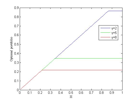
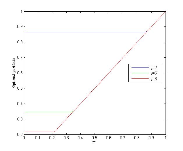
Figure 1: All Parameter values are given in (17). $\gamma=2$ and $\psi=1.2$ without special instructions. The discount rate $\delta=0.08$. They are both time-0 values for a problem with time horizon $T=30$ years.

Figure 1 shows the impact of the constraint on the optimal portfolio $\pi^{*}$ when we let $\Pi$ change with constraints $\pi\in[0,\Pi]$ and $\pi\in[\Pi,1]$ respectively. In Figure 1(a), the optimal portfolio $\pi^{*}$ increases when $\Pi$ increases until the optimal portfolio on $[0,1]$ is reached. After this $\pi^{*}$ does not change. In Figure 1(b), $\pi^{*}$ keeps the optimal portfolio on $[0,1]$ before this value and then increases as $\Pi$ increases. We can also get that the optimal portfolio $\pi^{*}$ on $[0,1]$ increases when $\gamma$ increases in both subfigures.

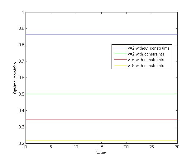
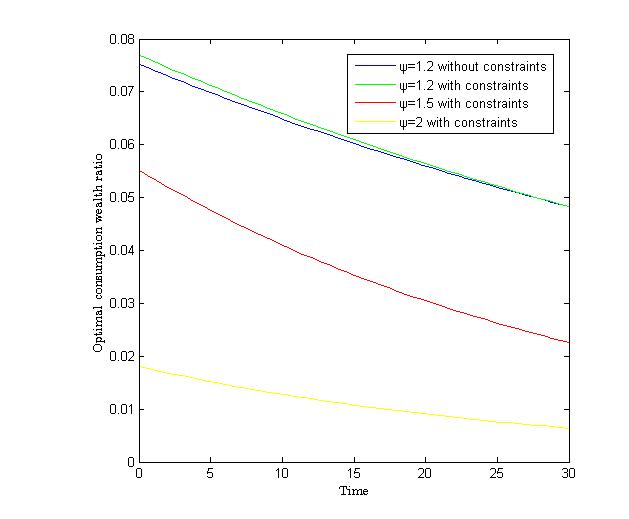
Figure 2: All Parameter values are given in (17). $\gamma=2$ and $\psi=1.2$ without special instructions. The time horizon is $T=30$ years. The discount rate $\delta=0.08$.

Then we consider the closed constraint $\pi\in[0,0.5]$. Figure 2 indicates that the closed constraint makes the optimal portfolio $\pi^{*}$ smaller and the optimal consumption wealth ratio $\hat{c}^{*}$ larger. But the change of $\hat{c}^{*}$ is not obvious. Figure 2(a) shows that $\pi^{*}$ is constant with respect to $t$. Besides, $\pi^{*}$ decreases as $\gamma$ increases and $\hat{c}^{*}$ decreases as $\psi$ increases when we consider constraints on $\pi^{*}$.

4.2 Linear diffusion model

The linear diffusion model, whose interest rate and the excess return of risky assets are linear functions. This model has been investigated in Campbell and Viceira (1999) for recursive utilities. In our situation, we truncate these linear functions to satisfy our assumptions as follows

$$\begin{dcases}dX_{t}=-bX_{t}dt+adW_{t},\\ dS_{t}=S_{t}\left[\left(r(X_{t})+\mu(X_{t})\right)dt+\sigma dW^{\rho}_{t}\right],\end{dcases}$$

where $r(x)=r_{0}+r_{1}((-100)\vee x)$, $\mu(x)=\sigma(\lambda_{0}+\lambda_{1}((-100)\vee x\wedge 100))$, given $b,a,\sigma,r_{0},r_{1},\lambda_{0},\lambda_{1},\rho,\rho^{\perp}\in\mathbb{R}$. These parameters satisfy the conditions in the following proposition.

Proposition 4.1.

Suppose $\gamma,\psi>1$ and

1. $b>0$, $a>0$,

2. $r_{1}>0$,

3. $\frac{a^{2}}{b}<\frac{1+\frac{4(1-\gamma)}{\gamma}\rho^{2}}{\left(\frac{2(1-\gamma)}{\gamma}\rho^{2}-1\right)^{2}}$,

4. $(\psi-1)r_{1}<\frac{(b-(\psi-1)a\lambda_{1}\rho)^{2}}{2a^{2}}$.

Then Theorem 3.2 holds.

This assumption ensures that X takes values in $E=\mathbb{R}$. The values of parameters are

$$r=0.0014,\lambda_{0}=0.05,\lambda_{1}=1,\sigma=0.0436,b=0.0226,a=0.0189,\rho=-0.935,\delta=0.0052,$$ (18)

which can be found in Wachter (2002). We consider the closed constraint $\pi\in[0,0.5]$.

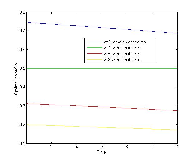
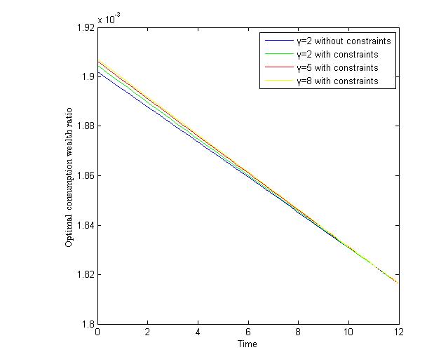
Figure 3: Each figure uses the parameters given in (18), $T=12$ month. Without special instructions, $\gamma=2$ and $\psi=1.2$.

Figure 3 compares the optimal portfolio $\pi^{*}$ and the optimal consumption wealth ratio $\hat{c}^{*}$ for portfolio strategies with and without closed constraints. Our numerical results show that the closed constraints has a significant impact on $\pi^{*}$ but hardly change $\hat{c}^{*}$. Two panels also illustrate the effects on $\pi^{*}$ and $\hat{c}^{*}$ for different risk aversion coefficients $\gamma$. When the risk aversion increases, the optimal portfolio is decreasing while the consumption wealth ratio is increasing.

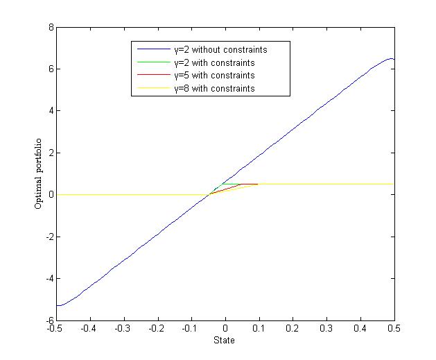
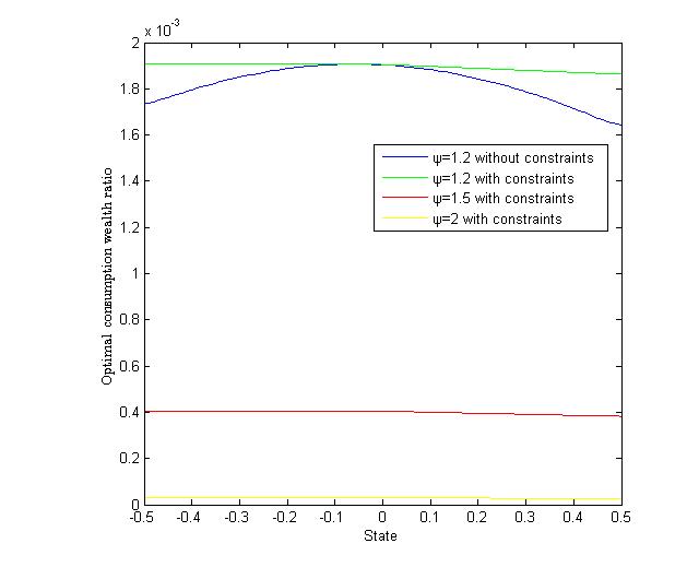
Figure 4: All Parameter values are given in (17). $\gamma=2$ and $\psi=1.2$ without special instructions. They are both time-0 values for a problem with the discount rate $\delta=0.08$.

Figure 4 compares the optimal portfolio $\pi^{*}$ and the optimal consumption wealth ratio $\hat{c}^{*}$ for portfolio strategies with and without closed constraints with respect to the state variable $X$. When we impose constraint $\pi\in[0,0.5]$, the part of $\pi^{*}$ greater than 0.5 takes 0.5 and the part less than 0 takes 0. In this case $\pi^{*}$ grows slower when $\gamma$ increases. It is shown in Figure 4(b) that $\hat{c}^{*}$ get smaller with respect to $\psi$ and is affected by state variable $X$ not obviously.

4.3 Stochastic volatility model

The state process $X$ is following a square root process, which is suggested by Heston and further investigated by Chacko and Viceira (2005),

$$\begin{dcases}dX_{t}=b(l-X_{t})dt+a\sqrt{X_{t}}dW_{t},\\ dS_{t}=S_{t}\left[\left(r(X_{t})+\mu(X_{t})\right)dt+\sigma(X_{t})dW^{\rho}_{t}\right],\end{dcases}$$

where $r(x)=r_{0}+r_{1}x$, $\mu(x)=\sigma\lambda x$, $\sigma(x)=\sigma x$, given $b,l,a,r_{0},r_{1},\sigma,\lambda,\rho,\rho^{\perp}\in\mathbb{R}$. These coefficients are subject to some restrictions in the following proposition.

Proposition 4.2.

Suppose $\gamma,\psi>1$ and

1. $b,l,a,r_{1},\sigma,\lambda>0,bl>\frac{1}{2}a^{2}$,

2. $\frac{1}{2}+\frac{2(1-\gamma)}{\gamma}|\rho|^{2}>0$,

3. $(\psi-1)r_{1}<\frac{b^{2}}{2a^{2}}$.

Then Theorem 3.2 holds.

Let us stress here that $X$ takes values in $(0,+\infty)$ with $E=(0,+\infty)$ and $r$ is bounded from below by $r_{0}$. Conditions in Proposition 4.2 already contain many empirically specifications in Liu and Pan (2003), where the values of these market parameters are

$$r=0.05,\ \lambda=0.47,\ l=0.0225,\ \sigma=1,\ b=5,\ a=0.25,\ \rho=-0.5,\ \delta=0.08.$$ (19)

Since the optimal portfolio $\pi^{*}$ without constraints lies in $[0,0.5]$, we choose portfolio constraint $\pi\in[0,0.1]$ in this model.

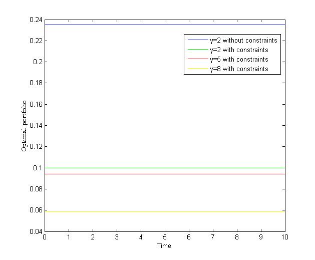
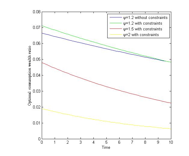
Figure 5: Parameter values are given in (19). Time horizon $T=10$ years. Without special instructions, $\gamma=2$ and $\psi=1.2$.

Figure 5 compares the optimal investment fraction $\pi^{*}$ and the optimal consumption wealth ratio $\hat{c}^{*}$ with respect to time $t$ for different values of the risk aversion $\gamma$ and the EIS $\psi$. It can be seen that $\gamma$ changes $\pi^{*}$ observably. Intuitively, an agent with larger risk aversion is more conservative and he will invest fewer wealth in risky asset. In Figure 5(b), the consumption wealth ratio is decreasing with respect to $\psi$. The figure also displays $\pi^{*}$ and $\hat{c}^{*}$ for portfolio strategies with and without closed constraints when $\gamma=2$ and $\psi=1.2$. Once we constrain the portfolio strategy, $\pi^{*}$ get smaller and $\hat{c}^{*}$ get bigger.

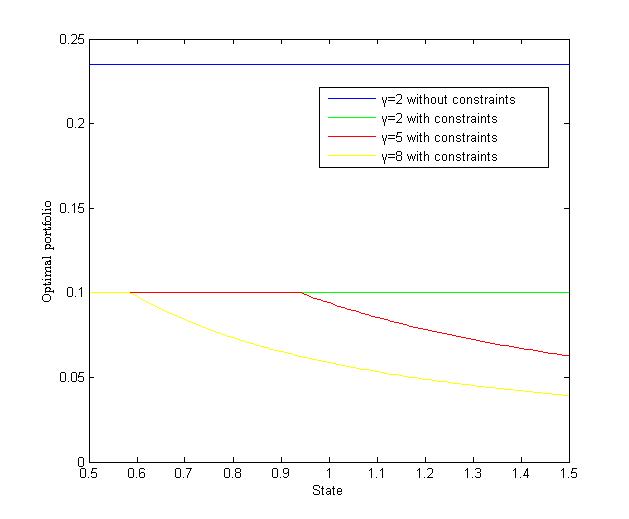
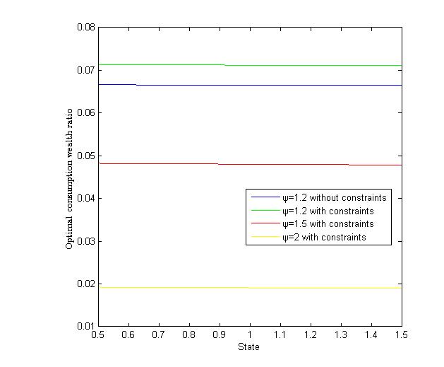
Figure 6: Parameter values are given in (19). Time horizon $T=10$ years. Without special instructions, $\gamma=2$ and $\psi=1.2$.

Figure 6 shows the optimal portfolio $\pi^{*}$ and the optimal consumption wealth ratio $\hat{c}^{*}$ with respect to the state variable $X$. Figure 6(b) depicts that $\hat{c}^{*}$ hardly changes depending on $X$. It becomes more complicated for $\pi^{*}$ as shown in Figure 6(a). When $\gamma=2$, $\pi^{*}$ remains 0.1; when $\gamma=5$ and 8, $\pi^{*}$ firstly stays constant and then decreases slowly.

5 The Proofs

5.1 Proof of Proposition 3.1

By Assumption 3.3, it implies that $\hat{W}:=W-\int_{0}^{\cdot}\frac{1-\gamma}{\gamma}\rho_{s}^{\prime}\sigma_{s}^{\prime}\Sigma_{s}^{-1}\mu_{s}ds$ is a Brownian motion under the new probability measure $\hat{\mathbb{P}}$. BSDE (9) then can be rewritten under $\hat{\mathbb{P}}$ as follows

$$\mathcal{Y}_{t}=\xi+\int_{t}^{T}\mathcal{H}(s,\mathcal{Y}_{s},Z_{s})ds-\int_{t}^{T}Z_{s}d\hat{W}_{s},\quad t\in[0,T],$$ (20)

where

$$\xi=\int_{0}^{T}\left(\frac{1-\gamma}{2\gamma}\mu_{s}^{\prime}\Sigma_{s}^{-1}\mu_{s}+(1-\gamma)r_{s}-\delta\theta\right)ds,$$

$$\mathcal{Y}_{t}=Y_{t}+\int_{0}^{t}\left(\frac{1-\gamma}{2\gamma}\mu_{s}^{\prime}\Sigma_{s}^{-1}\mu_{s}+(1-\gamma)r_{s}-\delta\theta\right)ds$$

and

$$\mathcal{H}(t,y,z)= -\frac{\gamma(1-\gamma)}{2}\operatorname{dist}^{2}\left(\mathcal{A}_{t},\frac{1}{\gamma}\sigma_{t}^{\prime}\Sigma_{t}^{-1}(\mu_{t}+\sigma_{t}\rho_{t}z^{\prime})\right)+z\big{(}\frac{1}{2}I_{k}+\frac{1-\gamma}{2\gamma}\rho_{t}^{\prime}\sigma_{t}^{\prime}\Sigma_{t}^{-1}\sigma_{t}\rho_{t}\big{)}z^{\prime}$$

$$+\frac{\theta}{\psi}\delta^{\psi}e^{-\frac{\psi}{\theta}y}\operatorname{exp}\left({\frac{\psi}{\theta}\int_{0}^{t}\left(\frac{1-\gamma}{2\gamma}\mu_{s}^{\prime}\Sigma_{s}^{-1}\mu_{s}+(1-\gamma)r_{s}-\delta\theta\right)ds}\right).$$

Similar to Proposition 2.9 in Xing (2017), by the localization technique in Briand and Hu (2006), for $m\geq 1$, we introduce $(\mathcal{Y}^{m},Z^{m})$ as the truncated version of BSDE (20),

$$\mathcal{Y}_{t}^{m}=\xi^{m}+\int_{t}^{T}\mathcal{H}^{m}(s,\mathcal{Y}_{s}^{m},Z_{s}^{m})ds-\int_{t}^{T}Z_{s}^{m}d\hat{W}_{s},\quad t\in[0,T],$$ (21)

where $\xi^{m}=\int_{0}^{T}\left(\frac{1-\gamma}{2\gamma}\mu_{s}^{\prime}\Sigma_{s}^{-1}\mu_{s}+(1-\gamma)(r_{s}\wedge m)-\delta\theta\right)ds$ and

$$\mathcal{H}^{m}(t,y,z)= -\frac{\gamma(1-\gamma)}{2}\operatorname{dist}^{2}\left(\mathcal{A}_{t},\frac{1}{\gamma}\sigma_{t}^{\prime}\Sigma_{t}^{-1}(\mu_{t}+\sigma_{t}\rho_{t}z^{\prime})\right)+z\big{(}\frac{1}{2}I_{k}+\frac{1-\gamma}{2\gamma}\rho_{t}^{\prime}\sigma_{t}^{\prime}\Sigma_{t}^{-1}\sigma_{t}\rho_{t}\big{)}z^{\prime}$$

$$+\frac{\theta}{\psi}\delta^{\psi}\left(e^{-\frac{\psi}{\theta}y}\wedge m\right)\operatorname{exp}\left({\frac{\psi}{\theta}\int_{0}^{t}\left(\frac{1-\gamma}{2\gamma}\mu_{s}^{\prime}\Sigma_{s}^{-1}\mu_{s}+(1-\gamma)(r_{s}\wedge m)-\delta\theta\right)ds}\right).$$

Since the eigenvalues of $\sigma^{\prime}\Sigma^{-1}\sigma$ are either 0 or 1, we obtain $0\leq\rho^{\prime}\sigma^{\prime}\Sigma^{-1}\sigma\rho\leq\rho^{\prime}\rho\leq I_{k}$. Then we get the following two inequalities

$$\frac{1}{2\gamma}I_{k}\leq\frac{1}{2}I_{k}+\frac{1-\gamma}{2\gamma}\rho^{\prime}\sigma^{\prime}\Sigma^{-1}\sigma\rho\leq\frac{1}{2}I_{k}$$ (22)

and

$$\operatorname{dist}^{2}\left(\mathcal{A}_{t},\frac{1}{\gamma}\sigma_{t}^{\prime}\Sigma_{t}^{-1}(\mu_{t}+\sigma_{t}\rho_{t}z^{\prime})\right)= \operatorname{min}_{p\in\mathcal{A}}\left|p-\frac{1}{\gamma}\sigma_{t}^{\prime}\Sigma_{t}^{-1}(\mu_{t}+\sigma_{t}\rho_{t}z^{\prime})\right|^{2}$$

$$\leq \frac{4}{\gamma^{2}}\mu_{t}^{\prime}\Sigma^{-1}_{t}\mu_{t}+\frac{4}{\gamma^{2}}z\rho_{t}^{\prime}\sigma_{t}^{\prime}\Sigma_{t}^{-1}\sigma_{t}\rho_{t}z^{\prime}+4\operatorname{min}_{p\in\mathcal{A}}|p|^{2}$$

$$\leq \frac{4}{\gamma^{2}}C_{0}+4C_{p}+\frac{4}{\gamma^{2}}zz^{\prime},$$ (23)

where the last inequality in (5.1) is deduced from Assumptions 3.1-3.2, (7) and (22).

According to (22), (7) and the fact that $\theta<0$, it implies that

$$\mathcal{H}^{m}(t,y,z) \leq\frac{5}{2}zz^{\prime}+2C_{0}+2\gamma(\gamma-1)C_{p}.$$ (24)

Thus $\mathcal{H}^{m}$ is Lipschitz continuous in $y$ with quadratic growth in $z$. It follows from Theorem 2.3 of Kobylanski (2000) that BSDE (21) admits a solution $(\mathcal{Y}^{m},Z^{m})\in\mathcal{S}^{\infty}\times\mathcal{M}^{2}$, where ${S}^{\infty}$ denotes the set of 1-dimensional continuous adapted processes $Y$ such that $||\sup_{0\leq s\leq T}|Y_{s}|||_{\infty}<+\infty$, and $\mathcal{M}^{2}$ denotes the set of predictable processes $Z$ such that $\hat{\mathbf{E}}\left(\int_{0}^{T}|Z_{s}|^{2}ds\right)<+\infty$.

Next, we will find a priori bound for $\mathcal{Y}^{m}$ independent of $m$. By (24), we consider

$$\overline{Y}_{t}^{m}=\xi^{m}+\int_{t}^{T}\frac{5}{2}{\overline{Z}_{s}^{m}}{\overline{Z}_{s}^{m}}^{\prime}+2C_{0}+2\gamma(\gamma-1)C_{p}ds-\int_{t}^{T}{\overline{Z}_{s}^{m}}d\hat{W}_{s},\quad t\in[0,T].$$

The explicit solution $\overline{Y}_{t}^{m}=\frac{1}{5}\ln\hat{\mathbf{E}}_{t}\left[\operatorname{exp}\left(5\xi^{m}+10(C_{0}+\gamma(\gamma-1)C_{p})T\right)\right]-2(C_{0}+\gamma(\gamma-1)C_{p})t.$ Since $r\geq r_{\operatorname{min}}$ and $\gamma>1$, then $\frac{1-\gamma}{2\gamma}\mu_{s}^{\prime}\Sigma_{s}^{-1}\mu_{s}+(1-\gamma)(r_{s}\wedge m)\leq(1-\gamma)r_{\operatorname{min}}.$ Thus,

$$\overline{Y}_{t}^{m} \leq[(1-\gamma)r_{\operatorname{min}}-\delta\theta+2(C_{0}+\gamma(\gamma-1)C_{p})]T-2(C_{0}+\gamma(\gamma-1)C_{p})t\leq C_{1}T$$

and

$$\overline{Y}_{t}^{m}-\int_{0}^{t}\left(\frac{1-\gamma}{2\gamma}\mu_{s}^{\prime}\Sigma_{s}^{-1}\mu_{s}+(1-\gamma)(r_{s}\wedge m)-\delta\theta\right)ds$$

$$= \frac{1}{5}\ln\hat{\mathbf{E}}_{t}\left[\operatorname{exp}\left(5\int_{t}^{T}\left(\frac{1-\gamma}{2\gamma}\mu_{s}^{\prime}\Sigma_{s}^{-1}\mu_{s}+(1-\gamma)(r_{s}\wedge m)-\delta\theta\right)ds+10(C_{0}+\gamma(\gamma-1)C_{p})T\right)\right]$$

$$-2(C_{0}+\gamma(\gamma-1)C_{p})t$$

$$\leq \frac{1}{5}\ln\hat{\mathbf{E}}_{t}\left[\operatorname{exp}\left(5[(1-\gamma)r_{\operatorname{min}}-\delta\theta](T-t)+10(C_{0}+\gamma(\gamma-1)C_{p})T\right)\right]-2(C_{0}+\gamma(\gamma-1)C_{p})t$$

$$= [(1-\gamma)r_{\operatorname{min}}-\delta\theta+2(C_{0}+\gamma(\gamma-1)C_{p})](T-t)$$

$$\leq C_{1}T.$$ (25)

Since $\theta<0$ and $\gamma>1$, by inequality (5.1), it derives that

$$\mathcal{H}^{m}(t,\overline{Y}_{t}^{m},\overline{Z}_{t}^{m})$$

$$\geq \frac{\theta}{\psi}\delta^{\psi}\operatorname{exp}\left(-\frac{\psi}{\theta}\left(\overline{Y}_{t}^{m}-\int_{0}^{t}\left(\frac{1-\gamma}{2\gamma}\mu_{s}^{\prime}\Sigma_{s}^{-1}\mu_{s}+(1-\gamma)(r_{s}\wedge m)-\delta\theta\right)ds\right)\right)$$

$$\geq \frac{\theta}{\psi}\delta^{\psi}\operatorname{exp}\left(-\frac{\psi}{\theta}C_{1}T\right).$$

Hence, we consider the following BSDE

$${\underline{Y}_{t}^{m}}=\xi^{m}+\frac{\theta}{\psi}\delta^{\psi}\operatorname{exp}\left(-\frac{\psi}{\theta}C_{1}T\right)(T-t)-\int_{t}^{T}{\underline{Z}_{s}^{m}}d\hat{W}_{s},$$

and it has an explicit form ${\underline{Y}_{t}^{m}}=\hat{\mathbf{E}}_{t}(\xi^{m})++\frac{\theta}{\psi}\delta^{\psi}\operatorname{exp}\left(-\frac{\psi}{\theta}C_{1}T\right)(T-t).$ It follows from the comparison theorem (Kobylanski (2000), Theorem 2.6), dominance convergence theorem and Assumption 3.3 that

$${\underline{Y}_{t}}\leq{\underline{Y}_{t}^{m}}\leq\mathcal{Y}_{t}^{m}\leq{\overline{Y}_{t}^{m}}\leq C_{1}T,$$

where

$$\underline{Y}_{t}=\hat{\mathbf{E}}_{t}(\xi)+\frac{\theta}{\psi}\delta^{\psi}\operatorname{exp}\left(-\frac{\psi}{\theta}C_{1}T\right)(T-t).$$

Using the localization technique introduced by Briand and Hu (2006), it implies the lower and upper bounds

$$\underline{Y}_{t}\leq\mathcal{Y}_{t}\leq\frac{1}{5}\ln\hat{\mathbf{E}}_{t}\left[\operatorname{exp}\left(5\xi+10(C_{0}+\gamma(\gamma-1)C_{p})T\right)\right]-2(C_{0}+\gamma(\gamma-1)C_{p})t.$$ (26)

Since $\mathcal{Y}_{T}=\xi$, subtracting $\int_{0}^{\cdot}\left(\frac{1-\gamma}{2\gamma}\mu_{s}^{\prime}\Sigma_{s}^{-1}\mu_{s}+(1-\gamma)r_{s}-\delta\theta\right)ds$ on both sides of (26), then

$$\mathcal{Y}_{t}-\int_{0}^{t}\left(\frac{1-\gamma}{2\gamma}\mu_{s}^{\prime}\Sigma_{s}^{-1}\mu_{s}+(1-\gamma)r_{s}-\delta\theta\right)ds$$

$$\geq \hat{\mathbf{E}}_{t}\left(\int_{t}^{T}\left(\frac{1-\gamma}{2\gamma}\mu_{s}^{\prime}\Sigma_{s}^{-1}\mu_{s}+(1-\gamma)r_{s}-\delta\theta\right)ds\right)+\frac{\theta}{\psi}\delta^{\psi}\operatorname{exp}\left(-\frac{\psi}{\theta}C_{1}T\right)(T-t)$$

$$\geq (1-\gamma)\hat{\mathbf{E}}_{t}\left[\int_{t}^{T}r_{s}ds\right]+C_{2}(t)$$

and

$$\mathcal{Y}_{t}-\int_{0}^{t}\left(\frac{1-\gamma}{2\gamma}\mu_{s}^{\prime}\Sigma_{s}^{-1}\mu_{s}+(1-\gamma)r_{s}-\delta\theta\right)ds$$

$$\leq \frac{1}{5}\ln\hat{\mathbf{E}}_{t}\left[\operatorname{exp}\left(5\int_{t}^{T}\left((1-\gamma)r_{\operatorname{min}}-\delta\theta\right)ds+10(C_{0}+\gamma(\gamma-1)C_{p})T\right)\right]-2(C_{0}+\gamma(\gamma-1)C_{p})t$$

$$\leq C_{1}T.$$

Therefore,

$$(1-\gamma)\hat{\mathbf{E}}_{t}\left[\int_{t}^{T}r_{s}ds\right]+C_{2}(t)\leq Y_{t}\leq C_{1}T,\qquad\forall t\in[0,T].$$

As for the square integrability of $Z$, taking a stopping time sequence $\tau_{n}\to T$, we can obtain that

$$\hat{\mathbf{E}}\left(\int_{0}^{\tau_{n}}Z_{s}\big{(}\frac{1}{2}I_{k}+\frac{1-\gamma}{2\gamma}\rho_{s}^{\prime}\sigma_{s}^{\prime}\Sigma_{s}^{-1}\sigma_{s}\rho_{s}\big{)}Z^{\prime}_{s}ds\right)$$

$$\leq\mathcal{Y}_{0}-\hat{\mathbf{E}}\left(\mathcal{Y}_{\tau_{n}}\right)-\hat{\mathbf{E}}\left[\int_{0}^{\tau_{n}}\frac{\theta}{\psi}\delta^{\psi}e^{-\frac{\psi}{\theta}\mathcal{Y}_{s}}\operatorname{exp}\left({\frac{\psi}{\theta}\int_{0}^{s}\left(\frac{1-\gamma}{2\gamma}\mu_{u}^{\prime}\Sigma_{u}^{-1}\mu_{u}+(1-\gamma)r_{u}-\delta\theta\right)du}\right)ds\right].$$

Applying (22), the upper bound and the lower estimate of $\mathcal{Y}$ in (26), when $n\to+\infty$ yields

$$\hat{\mathbf{E}}\left(\int_{0}^{T}|Z_{s}|^{2}ds\right)<+\infty.$$

$\hfill\Box$

5.2 Proof of Theorem 3.1

This proof is similar to Proposition 2.2 and Lemma B.1 in Xing (2017). Recall the definition of Epstein-Zin utility from (1), for each $(c,p)\in\mathcal{S}_{a}$,

$$V_{\cdot}^{c}+\int_{0}^{\cdot}f(c_{s},V_{s}^{c})ds$$

is a local martingale by Proposition 2.2 in Xing (2017). Define $Y_{t}^{c}:=(1-\gamma)e^{-\delta\theta t}V_{t}^{c}$, using Itô’s formula it implies that

$$Y_{\cdot}^{c}+\int_{0}^{\cdot}F(c_{s},Y_{s}^{c})ds$$ (27)

is also a local martingale, where $F(c_{t},y)=\delta\theta e^{-\delta t}c_{t}^{1-\frac{1}{\psi}}y^{1-\frac{1}{\theta}}$ is decreasing with $y$.

Let $\overline{V}^{c}:=\frac{\mathcal{W}^{1-\gamma}}{1-\gamma}e^{Y}$. From (9), it implies that $G_{\cdot}^{c,p}=\overline{V}_{\cdot}^{c}+\int_{0}^{\cdot}f(c_{s},\overline{V}_{s}^{c})ds$ is a local supermartingale. We claim that

$$\overline{Y}_{\cdot}^{c}+\int_{0}^{\cdot}F(c_{s},\overline{Y}_{s}^{c})ds$$ (28)

is a local submartingale, where $\overline{Y}_{t}^{c}=(1-\gamma)e^{-\delta\theta t}\overline{V}_{t}^{c}$. Indeed, taking an appropriate stopping time sequence $\{\tau_{n},n\geq 1\}$ with $\tau_{n}\stackrel{{\scriptstyle a.s.}}{{\longrightarrow}}T$, we obtain

$$\overline{V}_{t}^{c}+\int_{0}^{t}f(c_{s},\overline{V}_{s}^{c})ds\geq\mathbb{E}_{t}\left[\int_{0}^{\tau_{n}}f(c_{s},\overline{V}_{s}^{c})ds+\overline{V}_{\tau_{n}}^{c}\right],\quad t\in[0,\tau_{n}].$$

There exists an increasing process $A$ and a local square integrable process $\hat{Z}$ determined by the Doob-Meyer decomposition and the martingale representation theorem (Theorem 16 in Chapter III, and Theorem 43 in Chapter IV from Protter (2005)), such that

$$\overline{V}_{t}^{c}+\int_{0}^{t}f(c_{s},\overline{V}_{s}^{c})ds+A_{t}=\overline{V}_{0}^{c}+\int_{0}^{t}\hat{Z}_{s}dB_{s},\qquad t\in[0,\tau_{n}].$$

It implies the following BSDE

$$\overline{V}_{t}^{c}=\overline{V}_{\tau_{n}}^{c}+\int_{t}^{\tau_{n}}f(c_{s},\overline{V}_{s}^{c})ds+A_{\tau_{n}}-A_{t}-\int_{t}^{\tau_{n}}\widehat{Z}_{s}dB_{s},\quad t\in[0,\tau_{n}].$$

Applying It$\rm\hat{o}$’s formula to $(1-\gamma)e^{-\delta\theta t}\overline{V}_{t}^{c}$ yields

$$\overline{Y}_{t}^{c}=\overline{Y}_{\tau_{n}}^{c}+\int_{t}^{\tau_{n}}F(c_{s},\overline{Y}_{s}^{c})ds+(1-\gamma)e^{-\delta\theta t}(A_{\tau_{n}}-A_{t})-\int_{t}^{\tau_{n}}\widehat{Z}_{s}dB_{s},\quad t\in[0,\tau_{n}].$$

Therefore,

$$\overline{Y}_{t}^{c}+\int_{0}^{t}F(c_{s},\overline{Y}_{s}^{c})ds\leq\mathbb{E}_{t}\left[\int_{0}^{\tau_{n}}f(c_{s},\overline{Y}_{s}^{c})ds+\overline{Y}_{\tau_{n}}^{c}\right],\quad t\in[0,\tau_{n}].$$

Hence, the process (28) is a local submartingale.

Inspired by the third step of the proof of Proposition 2.2 in Xing (2017), define

$$\alpha_{t}:=\begin{cases}\frac{F(c_{t},\overline{Y}_{t}^{c})-F(c_{t},Y_{t}^{c})}{\overline{Y}_{t}^{c}-Y_{t}^{c}}\quad\rm{for}\ \overline{Y}_{t}^{c}\neq Y_{t}^{c},\\ 0\quad\rm{for}\ \overline{Y}_{t}^{c}=Y_{t}^{c}.\end{cases}$$

Since $y\mapsto F(\cdot,y)$ is nonincreasing, $\alpha\leq 0$. Comparing (27) and (28) we have

$$\overline{Y}_{t}^{c}-Y_{t}^{c}+\int_{0}^{t}F(c_{s},\overline{Y}_{s}^{c})-F(c_{s},Y_{s}^{c})ds=\overline{Y}_{t}^{c}-Y_{t}^{c}+\int_{0}^{t}\alpha_{s}\left(\overline{Y}_{s}^{c}-Y_{s}^{c}\right)ds.$$

It follows from It$\rm\hat{o}$’s formula and the class D property of $\overline{Y}^{c}$ and $Y^{c}$ that $e^{\int_{0}^{\cdot}\alpha_{s}ds}\left(\overline{Y}_{\cdot}^{c}-Y_{\cdot}^{c}\right)$ is a submartingale satisfying

$$\mathbb{E}_{t}\left[e^{\int_{0}^{T}\alpha_{s}ds}\left(\overline{Y}_{T}^{c}-Y_{T}^{c}\right)\right]\geq e^{\int_{0}^{t}\alpha_{s}ds}\left(\overline{Y}_{t}^{c}-Y_{t}^{c}\right).$$

Note that $\overline{Y}_{T}^{c}=Y_{T}^{c}$, we finally get

$$V_{t}^{c}\leq\frac{\mathcal{W}_{t}^{1-\gamma}}{1-\gamma}e^{Y_{t}}.$$

Moreover, since BSDE (9) has at least one solution, recall from (8) that

$$dG_{t}^{c,p}= \frac{\mathcal{W}_{t}^{1-\gamma}}{1-\gamma}e^{Y_{t}}\Bigg{[}\left(Z_{t}+(1-\gamma)p_{t}^{\prime}\rho_{t}\right)dW_{t}+(1-\gamma)p_{t}^{\prime}\rho_{t}^{\perp}dW_{t}^{\perp}$$

$$+\big{(}\delta\theta e^{-\frac{Y_{t}}{\theta}}\hat{c}_{t}^{1-\frac{1}{\psi}}-(1-\gamma)\hat{c}_{t}+(1-\gamma)p_{t}^{\prime}\sigma_{t}^{\prime}\Sigma_{t}^{-1}(\mu_{t}+\sigma_{t}\rho_{t}Z_{t})$$

$$-\frac{\gamma(1-\gamma)}{2})p_{t}^{\prime}p_{t}-H(\cdot,Y_{t},Z_{t})+(1-\gamma)r_{t}-\delta\theta+\frac{1}{2}Z_{t}Z_{t}^{\prime}\big{)}dt\Bigg{]}.$$ (29)

If $(c^{*},p^{*})\in\mathcal{S}_{a}$, then $\overline{V}^{c^{*}}+\int_{0}^{\cdot}f(c_{s}^{*},\overline{V}_{s}^{c^{*}})ds$ is a local martingale due to (10) and (5.2). Taking a localizing sequence $(\sigma_{n})_{n\geq 1}$, we have

$$\overline{V}_{0}^{c^{*}}+\delta\theta\mathbf{E}\left[\int_{0}^{T\wedge\sigma_{n}}\overline{V}_{s}^{c^{*}}ds\right]=\mathbf{E}\left[\overline{V}_{T\wedge\sigma_{n}}^{c^{*}}+\int_{0}^{T\wedge\sigma_{n}}\delta\frac{\left(c_{s}^{*}\right)^{1-\frac{1}{\psi}}}{1-\frac{1}{\psi}}\left((1-\gamma)\overline{V}_{s}^{c^{*}}\right)^{1-\frac{1}{\theta}}ds\right].$$

Since $\overline{V}^{c^{*}}\leq 0$ and $\psi>1$, the integrand on the left side of the equality is nonpositive and the integrand on the right side is nonnegative. Therefore, the class D property of $\overline{V}^{c^{*}}$ and the monotone convergence theorem imply that

$$\mathbf{E}\left[\int_{0}^{T}f\left(c_{s}^{*},\frac{\left(\mathcal{W}_{s}^{*}\right)^{1-\gamma}}{1-\gamma}e^{Y_{s}}\right)ds+\frac{\left(\mathcal{W}_{T}^{*}\right)^{1-\gamma}}{1-\gamma}\right]=\frac{\omega^{1-\gamma}}{1-\gamma}e^{Y_{0}}.$$

In this way, we confirm that $\frac{\omega^{1-\gamma}}{1-\gamma}e^{Y_{0}}$ is the optimal utility. Then the corresponding strategy $(c^{*},p^{*})$ is the optimal strategy for the problem (6). $\hfill\Box$

5.3 Proof of Theorem 3.2

According to the definition of $W^{\rho}$, we have

$$(1-\gamma)(p^{*})^{\prime}dW^{\rho}+ZdW$$

$$= \left((1-\gamma)(p^{*})^{\prime}\rho+Z\right)dW+(1-\gamma)(p^{*})^{\prime}\rho^{\perp}dW^{\perp}$$

$$=: M^{(1)}dW+M^{(2)}dW^{\perp}.$$

Bear in mind that the randomness of market parameters comes only from $W$, so we start with $\mathscr{E}\left(\int M^{(1)}dW\right)$. Define a stopping time sequence $\tau_{n}:=\inf\left\{t\geq 0:X_{t}\notin E_{n}\right\}\wedge T$. Now we claim that $Y_{\cdot\wedge\tau_{n}}$ is bounded. Combined with Proposition 3.1, it is sufficient to prove that $\hat{\mathbf{E}}_{\cdot\wedge\tau_{n}}\left[\int_{\cdot\wedge\tau_{n}}^{T}r_{s}ds\right]$ is bounded from above. Similar to Xing (2017), using Theorem 1 of Heath and Schweizer (2000), the Feynman-Kac formula guarantees that

$$y(t,x):=\hat{\mathbf{E}}\left(\int_{t}^{T}r_{s}ds\Big{|}X_{t}=x\right),\quad t\in[0,T],x\in E$$

is in $C^{1,2}([0,T]\times E)$ and $y$ is the unique solution to the following PDE

$$\begin{dcases}&\partial_{t}y+\mathscr{L}y+r=0,\\ &y(T,x)=0,\end{dcases}$$

where $\mathscr{L}$ is the infinitesimal generator of $X$ under $\hat{\mathbb{P}}$. Hence $y(\cdot\wedge\tau_{n},X_{\cdot\wedge\tau_{n}})=\hat{\mathbf{E}}_{\cdot\wedge\tau_{n}}\left[\int_{\cdot\wedge\tau_{n}}^{T}r_{s}ds\right]$ is bounded due to the compactness of $\overline{E}_{n}$. Consider the following truncated BSDE,

$$Y_{t}=Y_{\tau_{n}}+\int_{t}^{\tau_{n}}H(s,Y_{s},Z_{s})ds-\int_{t}^{\tau_{n}}Z_{s}dW_{s},\quad t\in[0,\tau_{n}].$$

By Assumption 3.2, $Y_{\cdot\wedge\tau_{n}}$ is then bounded. Since $H$ has quadratic growth in $z$, then Lemma 3.1 in Morlais (2009) implies that $\int_{0}^{\cdot\wedge\tau_{n}}Z_{s}dW_{s}\in\operatorname{BMO}(\mathbb{P})$. Observe that there exist two constants $k_{1}(n)$ and $k_{2}(n)$ depending on $n$, such that for $t\in[0,\tau_{n}]$,

$$|p^{*}_{t}| \leq\left|p^{*}_{t}-\frac{1}{\gamma}\sigma_{t}^{\prime}\Sigma_{t}^{-1}(\mu_{t}+\sigma_{t}\rho_{t}Z^{\prime}_{t})\right|+\left|\frac{1}{\gamma}\sigma_{t}^{\prime}\Sigma_{t}^{-1}(\mu_{t}+\sigma_{t}\rho_{t}Z^{\prime}_{t})\right|$$

$$=\operatorname{min}_{p_{t}\in\mathcal{A}_{t}}\left|p_{t}-\frac{1}{\gamma}\sigma_{t}^{\prime}\Sigma_{t}^{-1}(\mu_{t}+\sigma_{t}\rho_{t}Z^{\prime}_{t})\right|+\left|\frac{1}{\gamma}\sigma_{t}^{\prime}\Sigma_{t}^{-1}(\mu_{t}+\sigma_{t}\rho_{t}Z^{\prime}_{t})\right|$$

$$\leq\operatorname{min}_{p_{t}\in\mathcal{A}_{t}}|p_{t}|+2\left|\frac{1}{\gamma}\sigma_{t}^{\prime}\Sigma_{t}^{-1}(\mu_{t}+\sigma_{t}\rho_{t}Z^{\prime}_{t})\right|$$ (30)

$$\leq k_{1}(n)+k_{2}(n)|Z_{t}|.$$

The last inequality follows from (7). This means that $\int_{0}^{\cdot\wedge\tau_{n}}p^{*}_{s}dW_{s}\in\operatorname{BMO}(\mathbb{P})$. Therefore, $\mathscr{E}\left(\int M^{(1)}dW\right)_{\cdot\wedge\tau_{n}}$ is a uniformly integrable $\mathbb{P}$-martingale by Theorem 2.3 in Kazamaki (1994). Therefore,

$$\frac{d\mathbb{P}^{n}}{d\mathbb{P}}:=\mathscr{E}\left(\int M^{(1)}dW\right)_{\tau_{n}}$$ (31)

defines a new probability measure $\mathbb{P}^{n}$ equivalent to $\mathbb{P}$ on $\mathscr{F}_{\tau_{n}}$. Then we characterize $\mathbb{P}^{n}$ with the following lemma.

Lemma 5.1.

Let Assumptions 3.1, 3.2, 3.3 and 3.4 hold. Then $\lim_{n\to\infty}\mathbb{P}^{n}\left(\tau_{n}<T\right)=0$.

Proof.  We rewrite (9) as follows

$$Y_{t}=Y_{0}-\int_{0}^{t}H(s,Y_{s},Z_{s})ds+\int_{0}^{t}Z_{s}dW_{s},\quad t\in[0,T].$$

Since $\phi\in C^{2}(E)$, applying It$\rm\hat{o}$’s formula to $\phi(X_{t})$, it yields that

$$\phi(X_{t})=\phi(x)+\int_{0}^{t}b_{s}^{\prime}\nabla\phi+\frac{1}{2}\sum_{i,j=1}^{k}A_{ij}\partial^{2}_{x_{i}x_{j}}\phi ds+\int_{0}^{t}\nabla\phi^{\prime}a_{s}dW_{s}.$$

From (31), $W^{n}:=W-\int_{0}^{\cdot}\left[(1-\gamma)\left(p_{s}^{*}\right)^{\prime}\rho_{s}+Z_{s}\right]ds$ is a Brownian motion on $[0,\tau_{n}]$ under $\mathbb{P}^{n}$, and we obtain that

$$Y_{t}-\phi(X_{t})$$

$$= Y_{0}-\phi(x)+\int_{0}^{t}-H(s,Y_{s},Z_{s})-b_{s}^{\prime}\nabla\phi-\frac{1}{2}\sum_{i,j=1}^{k}A_{ij}\partial^{2}_{x_{i}x_{j}}\phi ds+\int_{0}^{t}Z_{s}-\nabla\phi^{\prime}a_{s}dW_{s}$$

$$= Y_{0}-\phi(x)+\int_{0}^{t}\frac{\gamma(1-\gamma)}{2}\operatorname{dist}^{2}\left(\mathcal{A}_{s},\frac{1}{\gamma}\sigma_{s}^{\prime}\Sigma_{s}^{-1}(\mu_{s}+\sigma_{s}\rho_{s}Z_{s}^{\prime})\right)$$

$$-Z_{s}\left(\frac{1}{2}I_{k}+\frac{1-\gamma}{2\gamma}\rho_{s}^{\prime}\sigma_{s}^{\prime}\Sigma_{s}^{-1}\sigma_{s}\rho_{s}\right)Z_{s}^{\prime}-\frac{1-\gamma}{\gamma}\mu_{s}^{\prime}\Sigma_{s}^{-1}\sigma_{s}\rho_{s}Z_{s}^{\prime}-\frac{\theta}{\psi}\delta^{\psi}e^{-\frac{\psi}{\theta}Y_{s}}$$

$$-\frac{1-\gamma}{2\gamma}\mu_{s}^{\prime}\Sigma_{s}^{-1}\mu_{s}-(1-\gamma)r_{s}+\delta\theta-b_{s}^{\prime}\nabla\phi-\frac{1}{2}\sum_{i,j=1}^{k}A_{ij}\partial^{2}_{x_{i}x_{j}}\phi ds$$

$$+\int_{0}^{t}\left(Z_{s}-\nabla\phi^{\prime}a_{s}\right)\left(dW_{s}^{n}+\left[(1-\gamma)\left(p_{s}^{*}\right)^{\prime}\rho_{s}+Z_{s}\right]ds\right)$$

$$= Y_{0}-\phi(x)+\int_{0}^{t}\frac{\gamma(1-\gamma)}{2}\operatorname{dist}^{2}\left(\mathcal{A}_{s},\frac{1}{\gamma}\sigma_{s}^{\prime}\Sigma_{s}^{-1}(\mu_{s}+\sigma_{s}\rho_{s}Z_{s}^{\prime})\right)$$

$$+Z_{s}\left(\frac{1}{2}I_{k}-\frac{1-\gamma}{2\gamma}\rho_{s}^{\prime}\sigma_{s}^{\prime}\Sigma_{s}^{-1}\sigma_{s}\rho_{s}\right)Z_{s}^{\prime}+\left[(1-\gamma)\left(p_{s}^{*}\right)^{\prime}\rho_{s}-\frac{1-\gamma}{\gamma}\mu_{s}^{\prime}\Sigma_{s}^{-1}\sigma_{s}\rho_{s}-\nabla\phi^{\prime}a_{s}\right]Z_{s}^{\prime}$$

$$-(1-\gamma)\left(p_{s}^{*}\right)^{\prime}\rho_{s}a_{s}^{\prime}\nabla\phi-\frac{\theta}{\psi}\delta^{\psi}e^{-\frac{\psi}{\theta}Y_{s}}-\frac{1-\gamma}{2\gamma}\mu_{s}^{\prime}\Sigma_{s}^{-1}\mu_{s}-(1-\gamma)r_{s}+\delta\theta-b_{s}^{\prime}\nabla\phi$$

$$-\frac{1}{2}\sum_{i,j=1}^{k}A_{ij}\partial^{2}_{x_{i}x_{j}}\phi ds+\int_{0}^{t}\left(Z_{s}-\nabla\phi^{\prime}a_{s}\right)dW_{s}^{n}.$$

Different from the proof of Lemma B.2 in Xing (2017), since there is no explicit solution for $p^{*}$ due to closed constraints in our situation, we will perform more refined analysis and estimations for the drift term in the following.

For any $s\in[0,\tau_{n}]$, it implies from (7) that

$$\frac{\gamma(1-\gamma)}{2}\operatorname{dist}^{2}\left(\mathcal{A}_{s},\frac{1}{\gamma}\sigma_{s}^{\prime}\Sigma_{s}^{-1}(\mu_{s}+\sigma_{s}\rho_{s}Z_{s}^{\prime})\right)$$

$$= \frac{\gamma(1-\gamma)}{2}\min_{p_{s}\in\mathcal{A}_{s}}\left|p_{s}-\frac{1}{\gamma}\sigma_{s}^{\prime}\Sigma_{s}^{-1}(\mu_{s}+\sigma_{s}\rho_{s}Z_{s}^{\prime})\right|^{2}$$

$$\geq \frac{1-\gamma}{2\gamma}\Big{|}\sigma_{s}^{\prime}\Sigma_{s}^{-1}(\mu_{s}+\sigma_{s}\rho_{s}Z_{s}^{\prime})\Big{|}^{2}$$

$$= \frac{1-\gamma}{2\gamma}Z_{s}\rho_{s}^{\prime}\sigma_{s}^{\prime}\Sigma_{s}^{-1}\sigma_{s}\rho_{s}Z_{s}^{\prime}+\frac{1-\gamma}{\gamma}\mu^{\prime}_{s}\Sigma^{-1}_{s}\sigma_{s}\rho_{s}Z_{s}^{\prime}+\frac{1-\gamma}{2\gamma}\mu^{\prime}_{s}\Sigma^{-1}_{s}\mu_{s}.$$

Therefore,

$$Y_{t}-\phi(X_{t})$$

$$\geq Y_{0}-\phi(x)+\int_{0}^{t}\frac{1}{2}Z_{s}Z_{s}^{\prime}+\left[(1-\gamma)\left(p_{s}^{*}\right)^{\prime}\rho_{s}-\nabla\phi^{\prime}a_{s}\right]Z_{s}^{\prime}-(1-\gamma)\left(p_{s}^{*}\right)^{\prime}\rho_{s}a_{s}^{\prime}\nabla\phi$$

$$-\frac{\theta}{\psi}\delta^{\psi}e^{-\frac{\psi}{\theta}Y_{s}}-(1-\gamma)r_{s}+\delta\theta-b_{s}^{\prime}\nabla\phi-\frac{1}{2}\sum_{i,j=1}^{k}A_{ij}\partial^{2}_{x_{i}x_{j}}\phi ds+\int_{0}^{t}\left(Z_{s}-\nabla\phi^{\prime}a_{s}\right)dW_{s}^{n}.$$ (32)

Based on the inequality (5.3), for $t\in[0,T]$, we get

$$|p^{*}_{t}| \leq\min_{p_{t}\in\mathcal{A}_{t}}\left|p_{t}\right|+2\left|\frac{1}{\gamma}\sigma_{t}^{\prime}\Sigma_{t}^{-1}(\mu_{t}+\sigma_{t}\rho_{t}Z^{\prime}_{t})\right|\leq C_{p}+\frac{2}{\gamma}\left|\sigma_{t}^{\prime}\Sigma_{t}^{-1}\mu_{t}\right|+\frac{2}{\gamma}\left|\sigma_{t}^{\prime}\Sigma_{t}^{-1}\sigma_{t}\rho_{t}Z^{\prime}_{t}\right|.$$

Then from algebraic inequalities, it yields the following estimations

$$(p_{t}^{*})^{\prime}\rho_{t}Z_{t}^{\prime} \leq\left|(p_{t}^{*})^{\prime}\rho_{t}Z_{t}^{\prime}\right|\leq\left|p_{t}^{*}\right|\left|\rho_{t}\right|\left|Z_{t}\right|$$

$$\leq C_{p}\left|\rho_{t}\right|\left|Z_{t}\right|+\frac{2}{\gamma}\left|\sigma_{t}^{\prime}\Sigma_{t}^{-1}\mu_{t}\right|\left|\rho_{t}\right|\left|Z_{t}\right|+\frac{2}{\gamma}\left|\sigma_{t}^{\prime}\Sigma_{t}^{-1}\sigma_{t}\rho_{t}\right|\left|\rho_{t}\right|\left|Z_{t}\right|^{2}$$ (33)

and

$$(p_{t}^{*})^{\prime}\rho_{t}a_{t}^{\prime}\nabla\phi \geq-\left|(p_{t}^{*})^{\prime}\rho_{t}a_{t}^{\prime}\nabla\phi\right|\geq-\left|p_{t}^{*}\right|\left|\rho_{t}a_{t}^{\prime}\nabla\phi\right|$$

$$\geq-C_{p}\left|\rho_{t}a_{t}^{\prime}\nabla\phi\right|-\frac{2}{\gamma}\left|\sigma_{t}^{\prime}\Sigma_{t}^{-1}\mu_{t}\right|\left|\rho_{t}a_{t}^{\prime}\nabla\phi\right|-\frac{2}{\gamma}\left|\sigma_{t}^{\prime}\Sigma_{t}^{-1}\sigma_{t}\rho_{t}Z^{\prime}_{t}\right|\left|\rho_{t}a_{t}^{\prime}\nabla\phi\right|.$$ (34)

Plugging (5.3) and (5.3) into (5.3), it derives that

$$\frac{1}{2}Z_{t}Z_{t}^{\prime}+\left[(1-\gamma)\left(p_{t}^{*}\right)^{\prime}\rho_{t}-\nabla\phi^{\prime}a_{t}\right]Z_{t}^{\prime}-(1-\gamma)\left(p_{t}^{*}\right)^{\prime}\rho_{t}a_{t}^{\prime}\nabla\phi$$

$$\geq \frac{1}{2}Z_{t}Z_{t}^{\prime}+(1-\gamma)C_{p}|\rho_{t}||Z_{t}|+\frac{2(1-\gamma)}{\gamma}\left|\sigma_{t}^{\prime}\Sigma_{t}^{-1}\mu_{t}\right|\left|\rho_{t}\right|\left|Z_{t}\right|+\frac{2(1-\gamma)}{\gamma}\left|\sigma_{t}^{\prime}\Sigma_{t}^{-1}\sigma_{t}\rho_{t}\right|\left|\rho_{t}\right|\left|Z_{t}\right|^{2}$$

$$-\left|\nabla\phi^{\prime}a_{t}\right|\left|Z_{t}\right|+(1-\gamma)C_{p}\left|\rho_{t}a_{t}^{\prime}\nabla\phi\right|+\frac{2(1-\gamma)}{\gamma}\left|\sigma_{t}^{\prime}\Sigma_{t}^{-1}\mu_{t}\right|\left|\rho_{t}a_{t}^{\prime}\nabla\phi\right|$$

$$+\frac{2(1-\gamma)}{\gamma}\left|\sigma_{t}^{\prime}\Sigma_{t}^{-1}\sigma_{t}\rho_{t}\right|\left|\rho_{t}a_{t}^{\prime}\nabla\phi\right|\left|Z_{t}\right|$$

$$= \left(\frac{1}{2}+\frac{2(1-\gamma)}{\gamma}\left|\sigma_{t}^{\prime}\Sigma_{t}^{-1}\sigma_{t}\rho_{t}\right|\left|\rho_{t}\right|\right)\left|Z_{t}\right|^{2}+\bigg{(}(1-\gamma)C_{p}|\rho_{t}|+\frac{2(1-\gamma)}{\gamma}\left|\sigma_{t}^{\prime}\Sigma_{t}^{-1}\mu_{t}\right|\left|\rho_{t}\right|-\left|\nabla\phi^{\prime}a_{t}\right|$$

$$+\frac{2(1-\gamma)}{\gamma}\left|\sigma_{t}^{\prime}\Sigma_{t}^{-1}\sigma_{t}\rho_{t}\right|\left|\rho_{t}a_{t}^{\prime}\nabla\phi\right|\bigg{)}\left|Z_{t}\right|+\frac{2(1-\gamma)}{\gamma}\left|\sigma_{t}^{\prime}\Sigma_{t}^{-1}\mu_{t}\right|\left|\rho_{t}a_{t}^{\prime}\nabla\phi\right|+(1-\gamma)C_{p}\left|\rho_{t}a_{t}^{\prime}\nabla\phi\right|.$$

Therefore, we can get

$$Y_{t}-\phi(X_{t})$$

$$\geq Y_{0}-\phi(x)+\int_{0}^{t}\left(\frac{1}{2}+\frac{2(1-\gamma)}{\gamma}\left|\sigma_{s}^{\prime}\Sigma_{s}^{-1}\sigma_{s}\rho_{s}\right|\left|\rho_{s}\right|\right)\Bigg{(}|Z_{s}|$$

$$+\frac{(1-\gamma)C_{p}|\rho_{s}|+\frac{2(1-\gamma)}{\gamma}\left|\sigma_{s}^{\prime}\Sigma_{s}^{-1}\mu_{s}\right|\left|\rho_{s}\right|-\left|\nabla\phi^{\prime}a_{s}\right|+\frac{2(1-\gamma)}{\gamma}\left|\sigma_{s}^{\prime}\Sigma_{s}^{-1}\sigma_{s}\rho_{s}\right|\left|\rho_{s}a_{s}^{\prime}\nabla\phi\right|}{1+\frac{4(1-\gamma)}{\gamma}\left|\sigma_{s}^{\prime}\Sigma_{s}^{-1}\sigma_{s}\rho_{s}\right|\left|\rho_{s}\right|}\Bigg{)}^{2}$$

$$-\frac{\theta}{\psi}\delta^{\psi}e^{-\frac{\psi}{\theta}Y_{s}}-(1-\gamma)r_{s}+\delta\theta-b_{s}^{\prime}\nabla\phi-\frac{1}{2}\sum_{i,j=1}^{k}A_{ij}\partial^{2}_{x_{i}x_{j}}\phi$$

$$+\frac{2(1-\gamma)}{\gamma}\left|\sigma^{\prime}_{s}\Sigma_{s}^{-1}\mu_{s}\right|\left|\rho_{s}a_{s}^{\prime}\nabla\phi\right|+(1-\gamma)C_{p}\left|\rho_{s}a_{s}^{\prime}\nabla\phi\right|$$

$$-\frac{\left((1-\gamma)C_{p}|\rho_{s}|+\frac{2(1-\gamma)}{\gamma}\left|\sigma_{s}^{\prime}\Sigma_{s}^{-1}\mu_{s}\right|\left|\rho_{s}\right|-\left|\nabla\phi^{\prime}a_{s}\right|+\frac{2(1-\gamma)}{\gamma}\left|\sigma_{s}^{\prime}\Sigma_{s}^{-1}\sigma_{s}\rho_{s}\right|\left|\rho_{s}a_{s}^{\prime}\nabla\phi\right|\right)^{2}}{2+\frac{8(1-\gamma)}{\gamma}\left|\sigma_{s}^{\prime}\Sigma_{s}^{-1}\sigma_{s}\rho_{s}\right|\left|\rho_{s}\right|}ds$$

$$+\int_{0}^{t}\left(Z_{s}-\nabla\phi^{\prime}a_{s}\right)dW_{s}^{n}$$

$$\geq Y_{0}-\phi(x)+\int_{0}^{t}\left(-\frac{\theta}{\psi}\delta^{\psi}e^{-\frac{\psi}{\theta}Y_{s}}-(1-\gamma)r_{s}+\delta\theta-\mathfrak{F}\left(\phi\right)\right)ds+\int_{0}^{t}\left(Z_{s}-\nabla\phi^{\prime}a_{s}\right)dW_{s}^{n}.$$

The last inequality derives from the definition of $\mathfrak{F}$ and the fact that $\frac{1}{2}+\frac{2(1-\gamma)}{\gamma}\left|\sigma^{\prime}\Sigma^{-1}\sigma\rho\right|\left|\rho\right|>0$. Since $\theta<0$, $r$ is bounded from below, and $\mathfrak{F}$ is bounded from above, then we can find a negative constant $C_{3}$, such that,

$$Y_{\tau_{n}}-\phi(X_{\tau_{n}})\geq Y_{0}-\phi(x)+C_{3}\tau_{n}+\int_{0}^{\tau_{n}}\left(Z_{s}-\nabla\phi^{\prime}a_{s}\right)dW_{s}^{n}.$$ (35)

Then by Theorem 3.6 of Kazamaki (1994), $\int_{0}^{\cdot\wedge\tau_{n}}\left(Z_{s}-\nabla\phi^{\prime}a_{s}\right)dW_{s}^{n}\in\operatorname{BMO}(\mathbb{P}^{n})$. Taking expectation under $\mathbb{P}^{n}$ on both sides of (35), we obtain

$$\mathbf{E}^{\mathbb{P}^{n}}\left[Y_{\tau_{n}}-\phi(X_{\tau_{n}})\right]\geq Y_{0}-\phi(x)+C_{3}T>-\infty,\qquad\forall n.$$ (36)

On the other hand, by Proposition 3.1 and the definition of $\tau_{n}$, it derives

$$Y_{\tau_{n}}-\phi(X_{\tau_{n}})= Y_{\tau_{n}}-\phi(X_{\tau_{n}})\mathbb{I}_{\{\tau_{n}=T\}}-\phi(X_{\tau_{n}})\mathbb{I}_{\{\tau_{n}<T\}}$$

$$\leq C_{1}T-\operatorname{inf}_{x\in E_{n}}\phi(x)\mathbb{I}_{\{\tau_{n}=T\}}-\operatorname{inf}_{x\in\partial E_{n}}\phi(x)\mathbb{I}_{\{\tau_{n}<T\}}.$$

By Assumption 3.4(i), there exists a constant $C_{4}$ such that $\operatorname{inf}_{x\in E}\phi(x)\geq C_{4}$. Thus the previous inequality implies that

$$\mathbf{E}^{\mathbb{P}^{n}}\left[Y_{\tau_{n}}-\phi(X_{\tau_{n}})\right]\leq C_{1}T+|C_{4}|-\operatorname{inf}_{x\in\partial E_{n}}\phi(x)\mathbb{P}^{n}(\tau_{n}<T).$$

From inequality (36), Assumption 3.4(i) derives that $\mathbb{P}^{n}(\tau_{n}<T)\to 0$. $\hfill\Box$

Using Lemma 5.1, we can verify the martingale property of (13).

Lemma 5.2.

Let Assumptions 3.1, 3.2, 3.3 and 3.4 hold. Then $M$ is a $\mathbb{P}$-martingale.

Proof. By Lemma 5.1, we have

$$\mathbf{E}\left[\mathscr{E}\left(\int M^{(1)}_{s}dW_{s}\right)_{T}\right]$$

$$= \lim_{n\to\infty}\mathbf{E}\left[\mathscr{E}\left(\int M^{(1)}_{s}dW_{s}\right)_{\tau_{n}}\right]-\lim_{n\to\infty}\mathbf{E}\left[\mathscr{E}\left(\int M^{(1)}_{s}dW_{s}\right)_{\tau_{n}}\mathbb{I}_{\{\tau_{n}<T\}}\right]$$

$$= 1-\lim_{n\to\infty}\mathbb{P}^{n}\left(\tau_{n}<T\right)=1.$$

This implies the martingale property of $\mathscr{E}\left(\int M_{s}^{(1)}dW_{s}\right)$ on $[0,T]$. Then we can confirm that $M$ is a $\mathbb{P}$-martingale. In fact, letting $\mathcal{F}^{W}=\sigma\left(W_{s},s\in[0,T]\right)$, since $M^{(2)}$ is independent of $W^{\perp}$, Lemma 4.8 of Karatzas and Kardaras (2007) implies that for any $t\in[0,T]$,

$$\mathbf{E}\left(M_{t}\right) =\mathbf{E}\left[\mathscr{E}\left(\int M_{s}^{(1)}dW_{s}+\int M_{s}^{(2)}dW_{s}^{\perp}\right)_{t}\right]$$

$$=\mathbf{E}\left[\mathscr{E}\left(\int M_{s}^{(1)}dW_{s}\right)_{t}\mathbf{E}\left[\mathscr{E}\left(\int M_{s}^{(2)}dW_{s}^{\perp}\right)_{t}\big{|}\mathcal{F}^{W}\right]\right]$$

$$=\mathbf{E}\left[\mathscr{E}\left(\int M_{s}^{(1)}dW_{s}\right)_{t}\right]$$

$$=1.$$

$\hfill\Box$

Proof of Theorem 3.2. By Theorem 3.1, we only need to show $(c^{*},p^{*})\in\mathcal{S}_{a}$.

Firstly, $\left(\mathcal{W}^{*}\right)^{1-\gamma}e^{Y}$ is of class D. In fact, applying It$\rm\hat{o}$’s formula to $\left(\mathcal{W}^{*}\right)^{1-\gamma}e^{Y}$, we have

$$\left(\mathcal{W}_{t}^{*}\right)^{1-\gamma}e^{Y_{t}}=\omega^{1-\gamma}e^{Y_{0}}\operatorname{exp}\left(\int_{0}^{t}\left(\theta\delta-\theta\delta^{\psi}e^{-\frac{\psi}{\theta}Y_{s}}\right)ds\right)M_{t},$$ (37)

where $M$ is defined in (13). By Lemma 5.2, $M$ is of class D and other terms are bounded. Then $\left(\mathcal{W}^{*}\right)^{1-\gamma}e^{Y}$ is of class D on $[0,T]$.

Next, we claim $c^{*}\in\mathcal{C}_{a}$. Since $Y_{T}=0$ and $\left(\mathcal{W}^{*}\right)^{1-\gamma}e^{Y}$ is of class D, then $\mathbf{E}\big{[}(\mathcal{W}_{T}^{*})^{1-\gamma}\big{]}<\infty$. Moreover, $e^{-\delta t}(c_{t}^{*})^{1-\frac{1}{\psi}}=\delta^{\psi-1}e^{-\delta t-\frac{\psi-1}{\theta}Y_{t}}\left(\mathcal{W}_{t}^{*}\right)^{1-\frac{1}{\psi}}$, it is only to show $\mathbf{E}\big{[}\int_{0}^{T}(\mathcal{W}_{s}^{*})^{1-\frac{1}{\psi}}ds\big{]}<\infty.$

Indeed, Hölder inequality and Assumption 3.5 imply that

$$\mathbf{E}\left[\int_{0}^{T}\left(\mathcal{W}_{s}^{*}\right)^{1-\frac{1}{\psi}}ds\right]$$

$$= \int_{0}^{T}\mathbf{E}^{0}\left[\operatorname{exp}\left((1-\frac{1}{\psi})\int_{0}^{s}r_{u}du\right)\operatorname{exp}\left(-(1-\frac{1}{\psi})\int_{0}^{s}r_{u}du\right)\left(\mathcal{W}_{s}^{*}\right)^{1-\frac{1}{\psi}}\mathscr{E}\left(\int\lambda_{u}dW_{u}^{0}\right)_{T}\right]ds$$

$$\leq \int_{0}^{T}\mathbf{E}^{0}\left(\operatorname{exp}\left((1-\frac{1}{\psi})\int_{0}^{T}r_{u}^{+}du\right)\mathscr{E}\left(\int\lambda_{u}dW_{u}^{0}\right)_{T}\operatorname{exp}\left(-(1-\frac{1}{\psi})\int_{0}^{s}r_{u}du\right)\left(\mathcal{W}_{s}^{*}\right)^{1-\frac{1}{\psi}}\right)ds$$

$$\leq \mathbf{E}^{0}\left(\operatorname{exp}\left((\psi-1)\int_{0}^{T}r_{u}^{+}du\right)\mathscr{E}\left(\int\lambda_{u}dW_{u}^{0}\right)_{T}^{\psi}\right)^{\frac{1}{\psi}}\int_{0}^{T}\mathbf{E}^{0}\left(\operatorname{exp}\left(-\int_{0}^{s}r_{u}du\right)\mathcal{W}_{s}^{*}\right)^{1-\frac{1}{\psi}}ds.$$

The statement is then confirmed due to the supermartingale property of $\operatorname{exp}\left(-\int_{0}^{\cdot}r_{u}du\right)\mathcal{W}^{*}$ under $\mathbb{P}_{0}$ as well as Assumption 3.5. $\hfill\Box$

5.4 Proof of Proposition 4.1

In order to prove Proposition 4.1 and the sequent Proposition 4.2, we need a lemma about the Laplace transform of a square root process. One can refer to Equation 2.k of Pitman and Yor (1982) or Lemma C.1 of Xing (2017).

Lemma 5.3.

A square root process $X$ is given by

$$dX_{t}=(\alpha-\beta X_{t})dt+a\sqrt{X_{t}}dW_{t},$$

where $W$ is a 1-dimensional Brownian motion. If $\zeta<\frac{\beta^{2}}{2a^{2}}$, then for any $T\geq 0$, the Laplace transform

$$\mathbf{E}\left(e^{\zeta\int_{0}^{T}X_{s}ds}\Big{|}X_{0}=x\right)$$

is well defined.

Assumptions 3.3, 3.4 and 3.5 are all verified in what follows. Then Theorem 3.2 holds.

Step 1. Verification of Assumption 3.3. Note that

$$\mathscr{E}\left(\int\frac{1-\gamma}{\gamma}\mu\Sigma^{-1}\sigma\rho dW_{s}\right)_{T}=\mathscr{E}\left(\int\frac{1-\gamma}{\gamma}(\lambda_{0}+\lambda_{1}((-100)\vee X_{s}\wedge 100))\rho dW_{s}\right)_{T}.$$

Obviously, $\hat{\mathbb{P}}$ is well-defined. One can refer to Eq.(3.17) of Chapter 5 of Karatzas and Shreve (2006) for the integrability of $X$ because $X$ is another Ornstein-Uhlenbeck process with modified linear drift under $\hat{\mathbb{P}}$. Therefore, Assumption 3.3 is satisfied.

Step 2. Verification of Assumption 3.4. Considering $\phi(x)=c_{0}x^{2}$ for some fixed constant $c_{0}>0$, we can prove that $\phi(x)\nearrow+\infty$ as $|x|\nearrow+\infty$. Meanwhile the operator $\mathfrak{F}$ reads

$$\mathfrak{F}[\phi]=c_{0}\left(\frac{a^{2}\left(\frac{2(1-\gamma)\rho^{2}}{\gamma}-1\right)^{2}}{\frac{1}{2}+\frac{2(1-\gamma)\rho^{2}}{\gamma}}-2b\right)x^{2}+\text{lower order terms in x}.$$

Then sufficiently small positive constants $c_{0}$ lead to $\mathfrak{F}[\phi](x)\searrow-\infty$ as $x\searrow 0$ or $x\nearrow+\infty$ when Condition (iii) in Proposition 4.1 holds. Therefore $\mathfrak{F}[\phi]$ is bounded from above on $(0,+\infty)$.

Step 3. Verification of Assumption 3.5. In order to apply Lemma 5.3, we change the dynamics of $X$ to the following form

$$dX_{t}=-(b-(\psi-1)a\lambda_{1}\rho)X_{t}dt+ad\tilde{W}_{t}.$$

Let $Y:=X^{2}$, it thus has the dynamics

$$dY_{t}=(a^{2}-2(b-(\psi-1)a\lambda_{1}\rho)Y_{t})dt+2a\sqrt{Y_{t}}d\tilde{W}_{t},$$

where $\tilde{W}:=W_{0}+\int_{0}^{\cdot}(\psi-1)\lambda_{0}\rho ds$ is a $\tilde{\mathbb{Q}}$-Brownian motion and $\tilde{\mathbb{Q}}$ is defined as

$$\frac{d\tilde{\mathbb{Q}}}{d\mathbb{P}_{0}}=\mathscr{E}\left(-(\psi-1)\lambda_{0}\rho W_{T}\right).$$

According to Remark 3.3, for sufficiently small $\epsilon>0$, it remains to prove

$$\mathbf{E}^{0}\left[\operatorname{exp}\left((1+\epsilon)(\psi-1)\left(r_{0}^{+}T+r_{1}\int_{0}^{T}X_{s}^{+}ds\right)\right)\right]<+\infty.$$ (38)

In fact, Hölder inequality implies that for $p>0$,

$$\mathbf{E}^{0}\left[\operatorname{exp}\left((1+\epsilon)(\psi-1)r_{1}\int_{0}^{T}X_{s}^{+}ds\right)\right]$$

$$\leq \mathbf{E}^{0}\left[\operatorname{exp}\left((1+\epsilon)(\psi-1)r_{1}\left(\int_{0}^{T}X_{s}^{2}ds+\frac{1}{4}T\right)\right)\right]$$

$$= \mathbf{E}^{\tilde{\mathbb{Q}}}\left[\frac{d\mathbb{P}_{0}}{d\tilde{\mathbb{Q}}}\operatorname{exp}\left((1+\epsilon)(\psi-1)r_{1}\left(\int_{0}^{T}X_{s}^{2}ds+\frac{1}{4}T\right)\right)\right]$$

$$\leq \mathbf{E}^{\tilde{\mathbb{Q}}}\left[\left(\frac{d\mathbb{P}_{0}}{d\tilde{\mathbb{Q}}}\right)^{\frac{1+p}{p}}\right]^{\frac{p}{1+p}}\mathbf{E}^{\tilde{\mathbb{Q}}}\left[\operatorname{exp}\left((1+p)(1+\epsilon)(\psi-1)r_{1}\left(\int_{0}^{T}X_{s}^{2}ds+\frac{1}{4}T\right)\right)\right]^{\frac{1}{1+p}}.$$

The first expectation on the right-hand side is finite because of the fact that $\frac{d\mathbb{P}_{0}}{d\tilde{\mathbb{Q}}}$ has any finite moment. As for the second expectation, Lemma 5.3 leads to the inequality that for sufficiently small $p$ and $\epsilon$,

$$(\psi-1)r_{1}<\frac{4(b-(\psi-1)a\lambda_{1}\rho)^{2}}{8a^{2}}.$$

Note that this is Condition (iv) in Proposition 4.1. $\hfill\Box$

5.5 Proof of Proposition 4.2

It is clear that the statement of Theorem 3.2 holds when Assumptions 3.3, 3.4 and 3.5 are all verified.

Step 1. Verification of Assumption 3.3. Direct calculation indicates that

$$\mathscr{E}\left(\frac{1-\gamma}{\gamma}\mu\Sigma^{-1}\sigma\rho dW_{s}\right)_{T}=\mathscr{E}\left(\frac{1-\gamma}{\gamma}\lambda\rho dW_{s}\right)_{T}.$$

Hence $\hat{\mathbb{P}}$ is well-defined and $\hat{W}=W-\int_{0}^{\cdot}\frac{1-\gamma}{\gamma}\lambda\rho ds$ is a Brownian motion under $\hat{\mathbb{P}}$. In addition, it follows from

$$dX_{t}=\left(bl+\frac{1-\gamma}{\gamma}a\rho\lambda\sqrt{X_{t}}-bX_{t}\right)dt+a\sqrt{X_{t}}d\hat{W}_{t}$$

that $X_{t}-X_{0}\leq blt+\int_{0}^{t}a\sqrt{X_{t}}d\hat{W_{t}}$. Then we have $\hat{\mathbf{E}}\left(X_{t}-X_{0}\right)\leq blt$. Hence

$$\hat{\mathbf{E}}\left[\int_{0}^{T}r_{s}ds\right]=r_{0}T+r_{1}\int_{0}^{T}\hat{\mathbf{E}}[X_{s}]ds<+\infty.$$

Step 2. Verification of Assumption 3.4. It is easy to check that $\phi(x)\nearrow+\infty$ as $x\nearrow+\infty$ or $x\searrow 0$ when taking $\phi(x)=c_{1}x-c_{2}\ln x$, where $c_{1}$ and $c_{2}$ are both sufficiently small positive constants. Moreover, the operator $\mathfrak{F}$ can be written as

$$\mathfrak{F}[\phi]= blc_{1}+bc_{2}+\frac{\frac{2(1-\gamma)^{2}}{\gamma^{2}}\lambda^{2}\rho^{2}}{1+\frac{4(1-\gamma)}{\gamma}\rho^{2}}-\frac{a^{2}c_{1}c_{2}\left(\frac{2(1-\gamma)}{\gamma}\rho^{2}-1\right)^{2}}{1+\frac{4(1-\gamma)}{\gamma}\rho^{2}}+\frac{(1-\gamma)^{2}\rho^{2}C_{p}\left(C_{p}+\frac{4\lambda}{\gamma}\right)}{2\left(1+\frac{4(1-\gamma)}{\gamma}\rho^{2}\right)}$$

$$+c_{1}\left[\frac{\left(\frac{2(1-\gamma)}{\gamma}\rho^{2}-1\right)^{2}a^{2}c_{1}}{2+\frac{8(1-\gamma)}{\gamma}\rho^{2}}-b\right]x+c_{2}\left[\frac{\left(\frac{2(1-\gamma)}{\gamma}\rho^{2}-1\right)^{2}a^{2}c_{2}}{2+\frac{8(1-\gamma)}{\gamma}\rho^{2}}+\frac{a^{2}}{2}-bl\right]\frac{1}{x}$$

$$+\frac{\frac{4(1-\gamma)}{\gamma}|\lambda\rho a|\left(1+\frac{1-\gamma}{\gamma}\rho^{2}\right)-\frac{2(1-\gamma)^{2}}{\gamma}a|\rho|^{3}C_{p}-2(1-\gamma)a|\rho|C_{p}}{1+\frac{4(1-\gamma)}{\gamma}\rho^{2}}\Big{|}c_{1}\sqrt{x}-\frac{c_{2}}{\sqrt{x}}\Big{|}.$$

Due to $bl>\frac{a^{2}}{2}$, then sufficiently small positive constants $c_{1}$ and $c_{2}$ lead to $\mathfrak{F}[\phi](x)\searrow-\infty$ as $x\searrow 0$ or $x\nearrow+\infty$. Therefore $\mathfrak{F}[\phi]$ is bounded from above on $(0,+\infty)$.

Step 3. Verification of Assumption 3.5. According to Remark 3.3, we only need to prove that for sufficiently small $\epsilon>0$,

$$\mathbf{E}^{0}\left[\operatorname{exp}\left((1+\epsilon)(\psi-1)\int_{0}^{T}r_{s}^{+}ds\right)\right]$$

$$\leq \mathbf{E}^{0}\left[\operatorname{exp}\left((1+\epsilon)(\psi-1)\left(r_{0}^{+}T+r_{1}\int_{0}^{T}X_{s}ds\right)\right)\right]<+\infty$$

It remains to prove the integrability of $\operatorname{exp}\left((1+\epsilon)(\psi-1)r_{1}\int_{0}^{T}X_{s}ds\right)$ under $\mathbb{P}_{0}$ . Indeed, using Hölder inequality once again, for $1<p^{\prime},q^{\prime}<+\infty$ with $\frac{1}{p^{\prime}}+\frac{1}{q^{\prime}}=1$,

$$\mathbf{E}^{0}\left[\operatorname{exp}\left((1+\epsilon)(\psi-1)r_{1}\int_{0}^{T}X_{s}ds\right)\right]$$

$$= \mathbf{E}\left[\mathscr{E}\left(\int-\lambda dW_{s}^{\rho}\right)_{T}\operatorname{exp}\left((1+\epsilon)(\psi-1)r_{1}\int_{0}^{T}X_{s}ds\right)\right]$$

$$\leq \mathbf{E}\left[\mathscr{E}\left(\int-\lambda dW_{s}^{\rho}\right)_{T}^{p^{\prime}}\right]^{\frac{1}{p^{\prime}}}\mathbf{E}\left[\operatorname{exp}\left((1+\epsilon)q^{\prime}(\psi-1)r_{1}\int_{0}^{T}X_{s}ds\right)\right]^{\frac{1}{q^{\prime}}}.$$ (39)

Following the above inequalities, one can similarly show that $\mathscr{E}\left(\int-\lambda dW_{s}^{\rho}\right)^{p^{\prime}}$ is integrable. For the second expectation in (5.5), we can choose $p^{\prime}$,$q^{\prime}$ sufficiently close to 1 such that according to Lemma 5.3, if

$$(\psi-1)r_{1}<\frac{b^{2}}{2a^{2}},$$

the second term is finite. This is exactly Condition (iii) in Proposition 4.2. $\hfill\Box$

6 Conclusions

The paper investigates the optimal consumption-investment problem for an investor with Epstein-Zin utility under general constraints in an incomplete market. Closed constraints are imposed on strategies. Our method is based on BSDE techniques coming from Hu, Imkeller and Müller (2005) and Xing (2017). The optimal consumption and investment strategies are characterized via a quadratic BSDE. Comparing with Xing (2017), the BSDE derived by the martingale optimal principle is more complicated, while the upper boundedness of the solution still holds under appropriate assumptions. In our situation, the candidate optimal strategy cannot be explicitly expressed by $Z$. To obtain the verification theorem, we need to carry out more sophisticated estimations and delicately choose suitable Lyapunov function to overcome the difficulties. Several examples and numerical simulations for the optimal strategies are illustrated and discussed.

References

References

- Aurand and Huang (2021) Aurand, J., Huang, Y, 2021. Mortality and healthcare: a stochastic control analysis under Epstein-Zin preferences. SIAM J. Control Optim. 59, 4051-4080.
- Bansal (2007) Bansal, R., 2007. Long-run risks and financial markets. Fed. Reserve Bank St. Louis Rev. 89, 1-17.
- Bansal and Yaron (2004) Bansal, R., Yaron, A., 2004. Risks for the long run: a potential resolution of asset pricing puzzles. J. Finance 59, 1481-1509.
- Benzoni, Collin-Dufresne and Goldstein (2011) Benzoni, L., Collin-Dufresne, P., Goldstein, R., 2011. Explaining asset pricing puzzles associated with the 1987 market crash. J. Financ. Econ. 101, 552-573.
- Bian, Chen and Xu (2019) Bian, B., Chen, X., Xu, Z., 2019. Utility maximization under trading constraints with discontinuous utility. SIAM J. Financial Math. 10, 243-260.
- Björk, Murgoci and Zhou (2014) Björk, T., Murgoci, A., Zhou, X., 2014. Mean-variance portfolio optimization with state-dependent risk aversion. Math. Finance 24, 1-24.
- Briand and Hu (2006) Briand, P., Hu, Y., 2006. BSDE with quadratic growth and unbounded terminal value. Probab. Theory Relat. Fields 136, 604-618.
- Campbell and Viceira (1999) Campbell, J., Viceira, L., 1999. Consumption and portfolio decisions when expected returns are time varying. Q. J. Econ. 114, 433-495.
- Chacko and Viceira (2005) Chacko, G., Viceira, L., 2005. Dynamic consumption and portfolio choice with stochastic volatility in incomplete markets. Rev. Financ. Stud. 18, 1369-1402.
- Chassagneux and Richou (2016) Chassagneux, J., Richou, A., 2016. Numerical simulation of quadratic BSDEs. Ann. Appl. Probab. 26, 263-304.
- Cheridito and Hu (2011) Cheridito, P., Hu, Y., 2011. Optimal consumption and investment in incomplete markets with general constraints. Stoch. Dyn. 11, 283-299.
- Cheridito, Kupper and Vogelpoth (2015) Cheridito, P., Kupper, M., Vogelpoth, N., 2015. Conditional Analysis on , Set Optimization and Applications, Proceedings in Mathematics & Statistics, 2015, 151: 179-211.
- Cox and Huang (1989) Cox, J., Huang, C., 1989. Optimal consumption and portfolio policies when asset prices follow a diffusion process. J. Econ. Theory 49, 33-83.
- Cvitanic and Karatzas (1992) Cvitanic, J., Karatzas, I., 1992. Convex duality in constrained portfolio optimization. Ann. Appl. Probab. 2, 767-818.
- Duffie and Epstein (1992) Duffie, D., Epstein, L., 1992. Stochastic differential utility. Econometrica 60, 353-394.
- El Karoui, Peng and Quenez (2001) El Karoui, Peng, S., Quenez, M. C., 2001. A dynamic maximum principle for the optimization of recursive utilities under constraints. Ann. Appl. Probab. 11, 664-693.
- Epstein and Zin (1989) Epstein, L., Zin, S., 1989. Substitution, risk aversion, and the temporal behavior of consumption and asset returns: A theoretical framework. Econometrica 57, 937-969.
- Fan (2018) Fan, S., 2018. Existence, uniqueness and stability of solutions for multidimensional BSDEs with generators of one-sided Osgood type. J Theor. Probab. 31(3), 1860-1899.
- Fan, Hu and Tang (2020) Fan, S., Hu, Y. and Tang, S., 2020. On the uniqueness of solutions to quadratic BSDEs with non-convex generators and unbounded terminal conditions. Comptes Rendus Mathmatique 358, 227-235.
- Heath and Schweizer (2000) Heath, D., Schweizer, M., 2000. Martingales versus PDEs in finance: an equivalence result with examples. J. Appl. Probab. 37, 947-957.
- Hu, Imkeller and Müller (2005) Hu, Y., Imkeller, P., Müller, M., 2005. Utility maximization in incomplete markets. Ann. Appl. Probab. 15, 1691-1712.
- Karatzas and Kardaras (2007) Karatzas, I., Kardaras, C., 2007. The nmraire portfolio in semimartingale financial models. Finance Stoch. 11, 447-493.
- Karatzas, Lehoczky and Shreve (1987) Karatzas, I., Lehoczky, J. P., Shreve, S. E., 1987. Optimal portfolio and consumption decisions for a “small investor” on a finite horizon. SIAM J. Control Optim. 25, 1557-1586.
- Karatzas and Shreve (2006) Karatzas, I., Shreve, S., 2006. Brownian motion and stochastic calculus. Springer, Berlin.
- Kazamaki (1994) Kazamaki, N., 1994. Continuous Exponential Martingales and BMO. Lecture Notes in Mathematics, vol. 1579. Springer, Berlin.
- Kobylanski (2000) Kobylanski, M., 2000. Backward stochastic differential equations and partial differential equations with quadratic growth. Ann. Probab. 28, 558-602.
- Kraft, Seiferling and Seifried (2017) Kraft, H., Seiferling, T., Seifried, F. T., 2017. Optimal consumption and investment with Epstein-Zin recursive utility. Finance Stoch. 21, 187-226.
- Kraft, Seifried and Steffensen (2013) Kraft, H., Seifried, F. T., Steffensen, M., 2013. Consumption-portfolio optimization with recursive utility in incomplete markets. Finance Stoch. 17, 161-196.
- Kramkov and Schachermayer (1999) Kramkov, D., Schachermayer, W., 1999. The asymptotic elasticity of utility functions and optimal investment in incomplete markets. Ann. Appl. Probab. 9, 904-950.
- Liu and Pan (2003) Liu, J., Pan, J., 2003. Dynamic derivative strategies. J. Financ. Econ. 69, 401-430.
- Matoussi and Xing (2018) Matoussi, A., Xing, H., 2018. Convex duality for Epstein-Zin stochastic differential utility. Math. Finance. 28, 991-1019.
- Melnyk, Muhle-Karbe and Seifried (2020) Melnyk, Y., Muhle-Karbe, J., Seifried, F. T., 2020. Lifetime investment and consumption with recursive preferences and small transaction costs. Math. Finance 30, 1135-1167.
- Merton (1971) Merton, R. C., 1971. Optimum consumption and portfolio rules in a continuous-time model. J. Econom. Theory 3, 373-413.
- Morlais (2009) Morlais, M.-A., 2009. Quadratic BSDEs driven by a continuous martingale and applications to the utility maximization problem. Finance Stoch. 13, 121-150.
- Pham (2008) Pham, H., 2008. Continuous-time stochastic control and optimization with financial applications. Springer, Berlin.
- Pitman and Yor (1982) Pitman, J., Yor, M., 1982. A decomposition of Bessel bridges. Probab. Theory Relat. Fields 59, 425-457.
- Pliska (1986) Pliska, S., 1986. A stochastic calculus model of continuous trading: Optimal portfolios. Math. Oper. Research. 11, 371-382.
- Protter (2005) Protter, P. 2005. Stochastic Integration and Differential Equation, 2nd edn., vol. 21. Corrected 3-rd Printing, Stochastic Modeling and Applied Probability. Springer.
- Robertson and Xing (2017) Robertson, S., Xing, H., 2017. Long-term optimal investment in matrix valued factor models. SIAM J. Financial Math. 8, 400-434.
- Rouge and El Karoui (2000) Rouge, R., El Karoui, N., 2000. Pricing via utility maximization and entropy. Math. Finance 10, 259-276.
- Schroder and Skiadas (1999) Schroder, M., Skiadas, C., 1999. Optimal consumption and portfolio selection with stochastic differential utility. J. Econ. Theory 89, 68-126.
- Schroder and Skiadas (2003) Schroder, M., Skiadas, C., 2003. Optimal lifetime consumption-portfolio strategies under trading constraints and generalized recursive preferences. Stochastic Process. Appl. 108, 155-202.
- Schroder and Skiadas (2005) Schroder, M., Skiadas, C., 2005. Lifetime consumption-portfolio choice under trading constraints, recursive preferences, and nontradeable income. Stochastic Process. Appl. 115, 1-30.
- Stroock and Varadhan (2006) Stroock, D.W., Varadhan, S.R.S., 2006. Multidimensional Diffusion Processes. Classics in Mathematics. Springer, Berlin. Reprint of the 1997 edition.
- Wachter (2002) Wachter, J., 2002. Portfolio and consumption decisions under mean-reverting returns: an exact solution for complete markets. J. Financ. Quant. Anal. 37, 63-91.
- Wang, Wang and Yang (2016) Wang, C., Wang, N., Yang, J., 2016. Optimal consumption and savings with stochastic income and recursive utility. J. Econom. Theory 165, 292-331.
- Xing (2017) Xing, H., 2017. Consumption-investment optimization with Epstein-Zin utility in incomplete markets. Finance Stoch. 21, 227-262.