Unification of BL Lac objects, FR I and FR II(G) radio galaxies and Doppler factor Estimation for BL Lac Objects

Abstract

In this work, we collected a sample of BL Lacs, FR I and FR II(G) radio galaxies with available core and extended emissions from published works to discuss the unified schemes and estimate the Doppler factor for BL Lacs. Wilcoxon rank-sum test and Kolmogorov-Smirnov test both suggest that the probabilities for the distribution of the extended luminosity of BL Lacs and that of FR I and FR II(G) radio galaxies to be from the same parent distribution are $p_{\rm{WRS}}=0.779$ and $p_{\rm{K-S}}=0.326$, suggesting they are unified. Based on this unified schemes, we propose to estimate the Doppler factors for BL Lacs. Comparing the Doppler factor estimated by the fitting/regression method with those for the common sources in the literatures, we found a good linear correlation for common sources.

1 Introduction

Active Galactic Nuclei (AGNs) are a special class of galaxies, showing extreme observation properties. Blazars are the extreme class of AGNs, which can be subdivided into two subclasses because of their behavior of emission lines: BL Lacertae objects (BL Lacs) with weak or no emission line and flat-spectrum radio quasars (FSRQs) with strong ones. BL Lacs show some extreme observation properties such as rapid and high amplitude variation, high and variable polarization, very weak or no emission line features, superluminal motions, or even high energy $\gamma$-ray emissions (Stickel et al., 1991; Fan et al., 1999, 2002; Xiao et al., 2019). When the viewing angle between relativistic jet and line of sight is small, a Doppler beaming effect should be taken into considered. The observed flux density $S^{\rm{ob}}$ is enhanced by the Doppler factor, $S^{\rm{ob}}=S^{\rm{in}}\delta^{q}$, where $S^{\rm{in}}$ is the intrinsic flux density, and $\delta$ is a Doppler factor, $q=2+\alpha$ for a continuous jet, $q=3+\alpha$ for a spherical jet (Scheuer & Readhead, 1979), in which $\alpha$ is the spectral index ($S_{\nu}\propto v^{-\alpha}$, $S_{\nu}$ for the monochromatic flux density). The Doppler factor is important for emissions in BL Lacs, which is determined by velocity ($\beta$) and the viewing angle ($\theta$): $\delta=[\Gamma(1-\beta\cos\theta)]^{-1}$, where $\Gamma$ is the Lorentz factor, satisfying $\Gamma=1/\sqrt{1-\beta^{2}}$.

Some methods were proposed to estimate the Doppler factor (Ghisellini et al., 1993; Mattox et al., 1993; Lähteemäki & Valtaoja, 1999; Fan et al., 2013; Chen, 2018; Liodakis et al., 2018; Zhang et al., 2020). Ghisellini et al. (1993) adopted the synchrotron self-Compton (SSC) model and assumed the synchrotron high frequency cutoff as $10^{14}$Hz to obtain the Doppler factors. Their results show that the Doppler factors are the largest for core-dominated quasars, intermediate for BL Lacs, and the smallest for radio galaxies and lobe-dominated quasars. Lähteemäki & Valtaoja (1999) adopted a method using the total radio flux density variations to assess Doppler factors and found high-polarization quasars with higher Doppler factors, while BL Lacs and low-polarization quasars have smaller Doppler factors. Following Mattox et al. (1993), Fan et al. (2013) assumed the $\gamma$-ray timescale as one day and calculated the lower limit for $\gamma$-ray Doppler factors from X-ray and $\gamma$-ray emissions. Based on the spectral energy distributions (SEDs) model, Chen (2018) estimated the Doppler factors for a sample of 999 blazars. The Doppler factor of BL Lacs is significantly larger than that of FSRQs in the work by Chen (2018). Liodakis et al. (2018) analyzed and constrained the average equipartition brightness temperature ($T_{eq}$) of the whole sample same as those ($T_{eq}=2.78\times 10^{11}K$) of FSRQs to obtain Doppler factors for a larger sample of blazars, showing that blazars are strongly beamed sources with higher Doppler factor on average than that of radio galaxies and unclassified sources. Zhang et al. (2020) proposed a new method based on the correlation between $\gamma$-ray luminosity and broad-line region luminosity to estimate the Doppler factors for a sample of 350 blazars. We can see that different method gives different Doppler factor value because of the different assumption in the literatures. For instance, based on the SSC model, Ghisellini et al. (1993) obtained a Doppler factor of $\delta=2.1$ for the BL Lac 0716+714, while Hovatta et al. (2009) obtained $\delta=$ 10.9 using the radio variation and Liodakis et al. (2018) derived a Doppler factor $\delta$ = 31.3 by adopting the same intrinsic brightness temperature for all the samples.

Radio galaxies are also a subclass of AGNs. From a work by Fanaroff & Riley (1974), the radio galaxies are classified into two types, based on their luminosity and the morphology. For some sources, the radio luminosity is mainly from the central part, this radio galaxy is classified as class I, called as Fanaroff-Riley class I (FR I) radio galaxy; some sources that their radio luminosity is mainly from the outer edge of the galaxy, this type of radio galaxy is regarded as class II radio galaxies, and called as Fanaroff-Riley class II (FR II) radio galaxy (Fanaroff & Riley, 1974). The centeral compact core emission in FR I radio galaxies (hereafter FR Is) is found to be identified with strongly associated with optical synchrotron radiation, which is produced in the inner regions of the relativistic jet (Chiaberge et al., 1999). In addition, Verdoes et al. (2002) had analyzed a complete sample of 21 nearby FR Is and proposed that the radio and optical core emissions of these samples are likely synchrotron radiation from inner jet because (a) radio and optical core emission are closely correlated, (b) the radio to optical spectral indices are similar to those for extended optical jets, (c) there is a suggestive trend with independent estimates from jet orientation, (d) the residual for radio-H$\alpha+$[N II] core correlation and that for optical-H$\alpha+$[N II] core correlation are well correlated with each other. From the optical spectrum, FR II radio galaxy can be subdivided into two subclass: FR II(G) and FR II(Q). The FR II(G) radio galaxy shows its optical type as that of a galaxy, while the spectral type of FR II(Q) resemble an optical type of a quasar (Xie et al., 1993).

In the unification of AGNs, the viewing angle is invoked to explain the different observation properties of AGNs. It was proposed that BL Lacs and FR Is were unified, in this unified scheme, the FR Is are the parent population of the BL Lacs (Urry et al., 1991; Ghisellini et al., 1993; Urry & Padovani, 1995). Urry et al. (1991) discussed the unification of BL Lacs and FR Is by computing luminosity functions, and found this samples were consistent with the beaming hypothesis that the BL Lacs are FR Is seen face on. Ghisellini et al. (1993) computed the average Lorentz factor ($\Gamma=8.32$) and viewing angle ($\theta=11.8$) for a sample of BL Lacs, which are consistent with other results from the attempts to unify FR I/BL Lac schemes, suggesting that the FR Is should be the parent population of the BL Lacs. Meanwhile, some authors suggested that FR II radio galaxies may be a part of parent population for BL Lacs (Xie et al., 1993; Owen et al., 1996; Fan et al., 1997). Xie et al. (1993) discussed the unified schemes of 75 BL Lacs, 27 FR I and 45 FR II(G) radio galaxies (hereafter FR II(G)s) using the Hubble diagram, and found BL Lacs and FR Is and FR II(G)s fit the same Hubble relation very well, supporting the unified schemes of BL Lacs and FR Is should include the FR II(G)s.

Due to the unobservable characteristics, it is difficult to obtain the Doppler factor. The previous studies mentioned above used different hypothesis to assess the Doppler factor (Ghisellini et al., 1993; Mattox et al., 1993; Lähteemäki & Valtaoja, 1999; Fan et al., 2013; Chen, 2018; Liodakis et al., 2018; Zhang et al., 2020). In this sense, any method estimating the Doppler factor is important for AGN studying. In a two-component model (Urry & Shafer, 1984), the core with a relativistic jet plus extended component is considered, in which the core emission is enhanced by the Doppler beaming effect, while the extended component has no beaming effect and shows their intrinsic emission. Since the extended emissions are unbeamed, then we can discuss the relationship of the extended luminosity for BL Lacs and FR I with FR II(G) radio galaxies (hereafter FR I/II(G)s). If BL Lacs and FR I/II(G)s are unified with FR I/II(G)s being the parent population of BL Lacs, then based on this unified schemes, we assumed that the intrinsic core and extended luminosity of BL Lacs should follow the same correlation as that of FR I/II(G)s, then we can estimate the Doppler factor of BL Lacs by using the core to extended luminosity fitting/regression method or ratio method of FR I/II(G)s. The structure of this work is arranged as follows. In Sect. 2, the unified schemes for BL Lacs and FR I/II(G)s is discussed using Wilcoxon rank-sum (WRS) test and Kolmogorov-Smirnov (K-S) test. In Sect. 3, based on this unified model, we estimate the Doppler factor. In Sect. 4, some discussions are presented, and some conclusions are shown in Sect. 5.

2 Samples and unified schemes

2.1 Samples

In this work, we collected 297 BL Lacs, 87 FR Is and 41 FR II(G)s with core and extended fluxes or luminosities at 5 GHz from the literature and showed them in Table 1,

Table 1: The core and extended fluxes or luminosities of whole samples and the Doppler factor of BL Lacs.

Source	class	$z$	$S_{\rm{core}}$	$S_{\rm{ext}}$	Ref	$logL_{\rm{core}}$	$logL_{\rm{ext}}$	Ref	$\delta_{2}$	$\delta_{2}$	$\delta_{2}$	$\delta_{3}$	$\delta_{3}$	$\delta_{3}$
Name			(mJy)	(mJy)		(W Hz${}^{-1})$	(W Hz${}^{-1})$		($\alpha_{c}=0$	0.5	-0.5)	($\alpha_{c}=0$	0.5	-0.5)
(1)	(2)	(3)	(4)	(5)	(6)	(7)	(8)	(9)	(10)	(11)	(12)	(13)	(14)	(15)
0003+003	B	1.037	480	206	P19	27.17	26.81		18.74	10.43	49.79	7.06	5.34	10.43
0003-066	B	0.347	1850	1504.47	P19	26.73	26.64		12.55	7.57	29.16	5.40	4.24	7.57
0007+124	I	0.156	4	751.02	F11	23.47	25.75
0007+472	B	0.280	67	22	P19	25.17	24.69		7.69	5.11	15.17	3.90	3.21	5.11
0011+1853	B	0.473	140	104	P19	25.89	25.76		8.58	5.58	17.57	4.19	3.42	5.58
0013+790	II(G)	0.840	4.4	1028.6	F11	25.21	27.58
0021+055	B	2.050	28	53	P19	26.56	26.83		9.04	5.82	18.84	4.34	3.52	5.82
0029-271	B	0.333	11	105	P19	24.67	25.65		2.27	1.93	2.98	1.73	1.60	1.93
0032+595	B	0.086	44	5	P19	23.92	22.97		5.71	4.03	10.20	3.19	2.71	4.03
0033+156	B	1.162	125	28	P19	26.96	26.31		20.43	11.18	55.86	7.47	5.61	11.18
0038+328	II(G)	0.482	0.47	1199.53	NED	23.64	27.05
0039+398	I	0.109	1	225	P19	22.52	24.88
0043+008	B	2.149	2	2	P19	25.27	25.27		5.86	4.11	10.55	3.25	2.75	4.11
0044+193	B	0.181	7	17	P19	23.71	24.10		2.13	1.83	2.74	1.65	1.54	1.83
0048-09	B	0.634	887	108.45	F11	26.98	26.07		24.62	12.97	71.62	8.46	6.24	12.97
0052+251	B	0.154	1	1	P19	22.73	22.73		1.71	1.54	2.05	1.43	1.36	1.54
0053+260	I	0.195				23.00	25.04	F11
$\cdots$	$\cdots$	$\cdots$	$\cdots$	$\cdots$	$\cdots$	$\cdots$	$\cdots$	$\cdots$	$\cdots$	$\cdots$	$\cdots$	$\cdots$	$\cdots$	$\cdots$

Note: Col. 1 gives the source name, Col. 2 the classification, B for BL Lacs, I for FR I, II(G) for FR II(G), Col. 3 redshift, Col. 4 the core flux density at 5 GHz, Col. 5 the extended flux density at 5 GHz, Col. 6 the references for Col. 4 and 5, NED for NASA/IPAC Extragalactic Datebase, M93 for Morganti et al. (1993), PS93 for Perlman & Stocke (1993), K05 for Kovalev et al. (2005), K10 for Kharb et al. (2010), F11 for Fan et al. (2011), DM14 for Di Mauro et al. (2014), P19 for Pei et al. (2019), Col. 7 the core luminosity at 5 GHz, Col. 8 the extended luminosity at 5 GHz, Col.9 the references for Col. 7 and 8, Z95 for Zirbel & Baum (1995), B11 for Broderick & Fender (2011), Col. 10 the Doppler factor for $q=2$, $\alpha_{c}=0$, Col. 11 the Doppler factor for q=2, $\alpha_{c}=0.5$, Col. 12 the Doppler factor for $q=2$, $\alpha_{c}=-0.5$, Col. 13 the Doppler factor for $q=3$, $\alpha_{c}=0$, Col. 14 the Doppler factor for $q=3$, $\alpha_{c}=0.5$, Col. 15 the Doppler factor for $q=3$, $\alpha_{c}=-0.5$.

( A portion is shown here for guidance regarding its form and content. The Table 1 is published in its entirety in Appendix.)

in which the core and extended fluxes at 5 GHz are listed in Col. 3-4 with their references in Col. 5, and their corresponding luminosities are listed in Col. 7-8. For some sources, their core and extended luminosities are available in the literatures (Zirbel & Baum, 1995; Broderick & Fender, 2011; Fan et al., 2011) as listed in Col. 7-9. Generally, the measured frequency of data is different in different literature. Because most of the measured radio frequency is at 5 GHz, Fan et al. (2011) and Pei et al. (2019) transferred the data at other measured frequency to 5 GHz, $S^{5GHz}_{c}=S^{\nu,obs}_{c}$, $S_{ext}^{5GHz}=S_{\rm{ext}}^{\nu,obs}(\frac{\nu}{5GHz})^{\alpha_{\rm{ext}}}$, with $\alpha_{\rm{ext}}=0.75$ and $\alpha_{c}=0.0$ (Fan et al., 2011; Pei et al., 2019).

We compare BL Lacs in the present sample (BL Lacs_TW, 297 sources) with BL Lacs (BL Lacs_ref, 649 sources) in the references (Fan et al., 2011; Pei et al., 2019) and Roma-BZCAT (Massaro et al., 2015), to discuss the completeness of BL Lacs of the sample. The redshift of BL Lacs_TW is in the range of 0.026 to 3.2, and the coverage range for redshift distribution of BL Lacs_TW is similar to that of BL Lacs_ref,

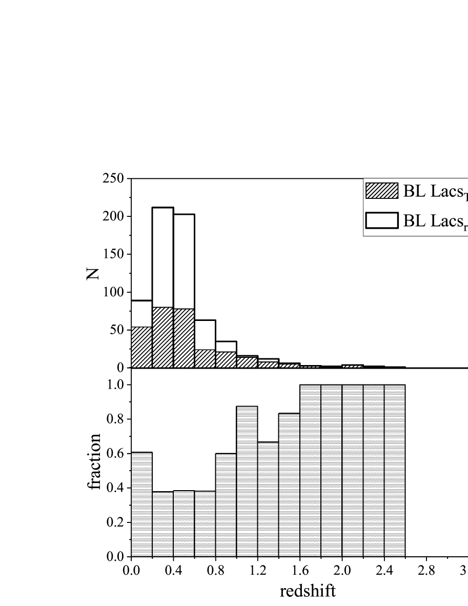
Figure 1: The upper panel is the redshift distributions for BL Lacs, the unhatched area for BL Lacs (BL Lacs_ref) in the references (Fan et al., 2011; Pei et al., 2019) and Roma-BZCAT (Massaro et al., 2015), the hatching area for BL Lacs in the present sample (BL Lacs${}_{\rm{TW}})$. The lower panel is the fraction between BL Lacs_TW and BL Lacs_ref in different redshift bin.

which is also in the range of 0.026 to 3.2, as shown in the upper panel of Fig. 1. Additionally, the fraction between BL Lacs_TW and BL Lacs_ref is obtained in different redshift bin and presented in the lower panel of Fig. 1. About half of BL Lacs_ref within redshift $<$ 1 and almost all the BL Lacs_ref with redshift $>$ 1 were selected for research. FR I/IIs in the present sample (FRs_TW, 128 sources) are also compared with FR I/IIs (FRs_ref, 395 sources) in the references (Mattox et al., 1993; Zirbel & Baum, 1995; Broderick & Fender, 2011; Fan et al., 2011; Pei et al., 2019). The redshift distribution of FRs_TW is in a range of 0.003 to 1.132, and that of FRs_ref ranges from 0.002 to 2.009, as shown in upper panel of Fig. 2. The fraction between FRs_TW and FRs_ref in different redshift bin is also presented in the lower panel of Fig. 2. One can see that the present sample has a smaller redshift than that from the references. We think that the reason is because the radio galaxy with higher redshift is weak so that it is hard for one to obtain the core and the extended emissions, therefore we can only separate the core and the extended emissions for the low redshift radio galaxy. We hope that we can obtain more core and extended emissions with higher redshift in the future.

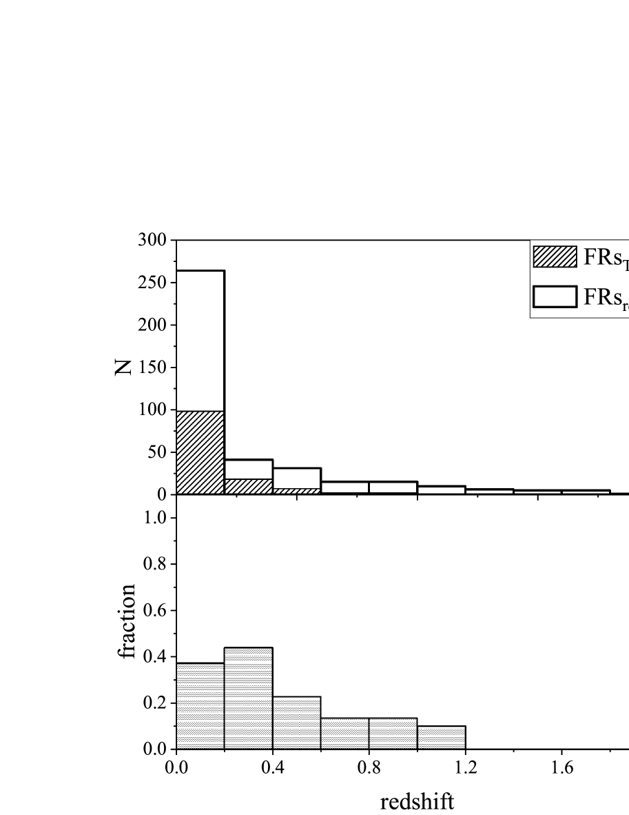
Figure 2: The upper panel is the redshift distributions for FR I/IIs, the unhatched area for FR I/IIs (FRs_ref) in the references (Mattox et al., 1993; Zirbel & Baum, 1995; Broderick & Fender, 2011; Fan et al., 2011; Pei et al., 2019), the hatching area for FR I/IIs in the present sample (FRs${}_{\rm{TW}})$. The lower panel is the fraction between FRs_TW and FRs_ref in different redshift bin.

2.2 Luminosity Calculation

From the core and extended fluxes, one can calculate the corresponding luminosities, $L=4\pi d_{L}^{2}S_{\nu}$, where $d_{L}$ is a luminosity distance expressed by

$$d_{L}=(1+z)\frac{c}{H_{0}}\int_{1}^{1+z}\frac{1}{\sqrt{\Omega_{M}x^{3}+1-\Omega_{M}}}dx$$ (1)

with $\Omega_{\Lambda}\sim 0.692$, $\Omega_{M}\sim 0.308$ and $H_{0}=67.8$km s^-1 Mpc^-1 (Planck Collaboration et al., 2016).

For the 297 BL Lacs, our calculation shows that the logarithm of the core luminosity, log$L_{\rm{core}}$, is in a range of $\log L_{\rm{core}}$ = 21.96 $--$ 28.70 with an average of 25.53, where $L_{\rm{core}}$ indicates the core luminosity in the unit of W Hz^-1, and that of the extended luminosity, log$L_{\rm{ext}}$, is in a range of $\log L_{\rm{ext}}$ = 21.56 $--$ 28.19, where $L_{\rm{ext}}$ indicates the extended luminosity in the unit of W Hz^-1.

For the 87 FR Is, we have $\log L_{\rm{core}}$ = 20.90 $--$ 25.40 with an average of 23.32 for the core luminosity, and $\log L_{\rm{ext}}$ = 22.49 $--$ 26.80 with an average of 24.43 for the extended luminosity. While for the 41 FR II(G)s, the core luminosity is found to be in a range from $\log L_{\rm{core}}$ = 22.69 $--$ 26.56 with an average of 24.43 and the extended luminosity in a range of $\log L_{\rm{ext}}$ = 25.14 $--$ 27.85 with an average of 26.35.

2.3 Unification Scheme

From the relativistic two-component model (Urry & Shafer, 1984), the total luminosity consists of the core (beamed) luminosity and extended (unbeamed) luminosity, in which core luminosity is enhanced by the relativistic beaming effect, while the extended luminosity displays its intrinsic value. In order to investigate the unification between BL Lacs and FR I/II(G)s, we used the extended luminosity for these samples. Because of the FR I/FR II dichotomy from the Fanaroff & Riley (1974), the different property in the luminosity between the FR I and FR II is widely accepted for decades. FR Is show their behavior as low radio power, and FR IIs behave as high radio power owing to their different jet effect. In our samples, the FR II(G)s have a higher extended luminosity

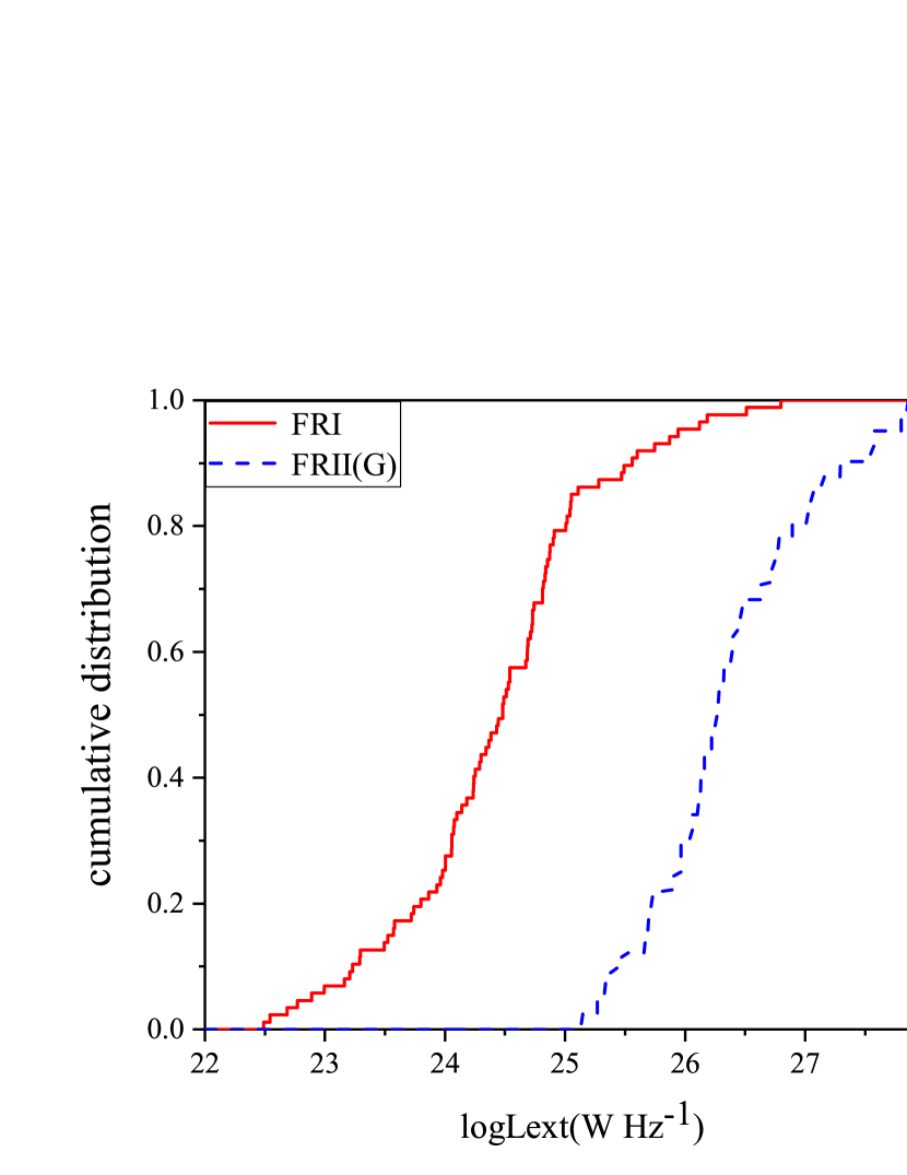
Figure 3: The cumulative distributions for extended luminosity of FR Is and FR II(G)s, in which the solid line represents FR Is and broken line represents FR II(G)s.

ranging from $\log L_{\rm{ext}}$ = 25.14 $--$ 27.85, but FR Is have lower extended luminosity, $\log L_{\rm{ext}}$ = 22.46 $--$ 26.80. The cumulative distributions for extended luminosity of FR Is and FR II(G)s are presented in Fig. 3.

As for BL Lacs and FR Is, the extended luminosity distribution of BL Lacs ($\log L_{\rm{ext}}$ = 21.56 $--$ 28.19) is wider than that of FR Is ($\log L_{\rm{ext}}$ = 22.49 $--$ 26.80) and BL Lacs have a higher average extended luminosity than that of FR Is. There is a marginal difference for low luminosity of BL Lacs and FR Is, but clear difference for high luminosity as shown in the left panel of Fig. 4, the probability values for the K-S test and WRS test are both $<10^{-4}$, in which the hypothesis for WRS test as did Liodakis et al. (2018) is to determine whether the two independent samples are from the same distribution and for K-S test is to discriminate between two statistical distributions, their p value threshold is taken as 0.05.

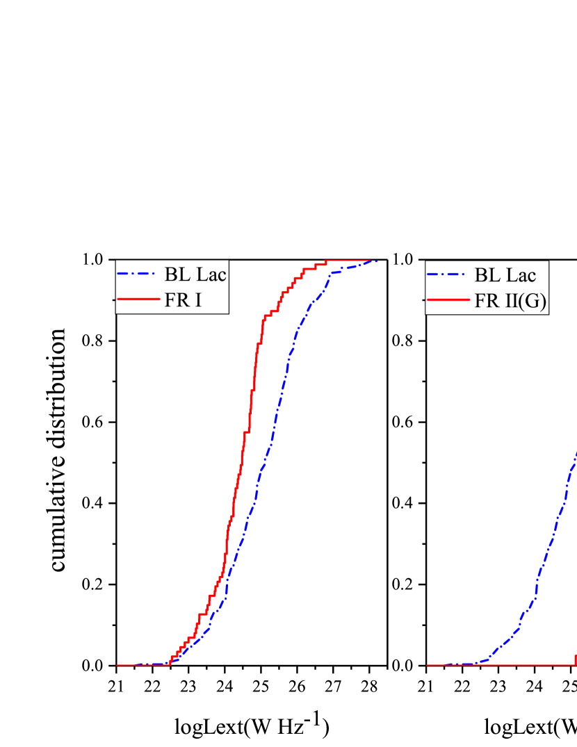
Figure 4: The left panel is the cumulative distributions for extended luminosity of BL Lacs and FR Is, in which the solid line represents FR Is and broken-dotted line represents BL Lacs. The right panel is the cumulative distributions for extended luminosity of BL Lacs and FR II(G)s, in which the solid line represents FR II(G)s and broken-dotted line represents BL Lacs.

The extended luminosities for BL Lacs and FR II(G)s are also discussed. The extended luminosities for FR II(G)s are almost the high luminosity ($\log L_{\rm{ext}}$ = 25.14 $--$ 27.85), so the cumulative distribution for extended luminosity of BL Lacs renders discrepant result from that of FR II(G)s with both p $<10^{-4}$ for K-S test and WRS test as shown in right panel of Fig. 4.

It is proposed that the FR Is and FR II(G)s are the parent population of BL Lacs as we mentioned above (Xie et al., 1993; Owen et al., 1996; Fan et al., 1997). If it is the case, one can expect that, for the extended luminosity, the distribution of FR I/II(G)s and that of BL Lacs should be from the same parent distribution. Now, we will investigate those distributions using WRS test and K-S test. For the FR I/II(G)s, the total extended luminosity is in a range of $\log L_{\rm{ext}}$ = 22.49 $--$ 27.85 with an average value 25.04, and their cumulative distribution for extended luminosity is close to that of BL Lacs, in which the corresponding cumulative distributions for extended luminosity of BL Lacs and FR I/II(G)s are shown in Fig. 55. When the WRS test and K-S test are adopted to the distribution of extended luminosity of BL Lacs and that of FR I/II(G)s, it is found that the probabilities for the both extended luminosities to be from the same parent distribution are $p_{\rm{WRS}}=0.779$ and $p_{\rm{K-S}}=0.326$, implying that the null hypothesis cannot be reject, suggesting that the extended luminosity distribution for BL Lacs and that of FR I/II(G)s are from the same parent distribution, which indicates that the BL Lacs and FR I/II(G)s are unified.

We also compared the core luminosity for BL Lacs and FR I/II(G)s. The total core luminosity for FR I/II(G)s is spanning from $\log L_{\rm{core}}$ = 20.90 to 26.56 with an average of 23.67, while the core luminosity for BL Lac is from $\log L_{\rm{core}}$ = 21.96 to 28.70 with an average of 25.53. The core luminosity distribution for FR I/II(G)s is significantly different from that of BL Lacs as presented in Fig. 55. Both the WRS test and K-S test give p $<10^{-4}$, showing that the core luminosity of BL Lacs and that of FR I/II(G)s are from different distributions. The discrepancy for core luminosity between BL Lacs and FR I/II(G)s is due to the strong beaming effect in BL Lacs.

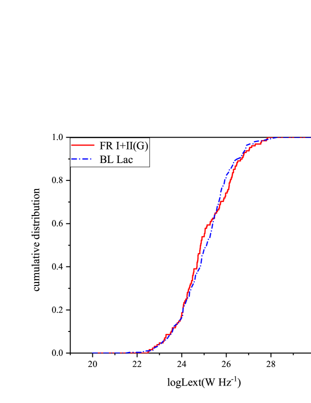
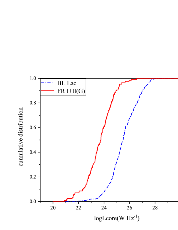
Figure 5: The cumulative distributions of BL Lacs and FR I/II(G)s: 5 for extended luminosity. 5 for core luminosity. The solid line represents the FR I/II(G)s, and the broken-dotted line represents the BL Lacs.

3 Estimation of Doppler Factor

3.1 Methodology

When the jet direction of a BL Lac is close to our line of sight, it causes a strong beaming effect for the core emission, $S^{\rm{ob}}_{\rm{core}}=\delta^{q}S^{\rm{in}}_{\rm{core}}$, where $S^{\rm{ob}}_{\rm{core}}$ and $S^{\rm{in}}_{\rm{core}}$ are the observed core flux density and the intrinsic core flux density of BL Lacs, $q=2+\alpha_{c}$ or $3+\alpha_{c}$ from different jet structure (Scheuer & Readhead, 1979), and $\alpha_{c}$ is the radio core spectral index of BL Lacs ($S_{\rm{core,\nu}}\propto\nu^{-\alpha_{c}}$). For luminosities, one can get $L_{\rm{BL,core}}^{\rm{ob}}=\delta^{q}L_{\rm{BL,core}}^{\rm{in}}$, in which the $L_{\rm{BL,core}}^{\rm{ob}}$ and $L_{\rm{BL,core}}^{\rm{in}}$ are the observed core luminosity and intrinsic core luminosity of BL Lacs.

As we mentioned in §2.3, BL Lacs and FR I/II(G)s are unified. In this sense, one can expect that the intrinsic luminosity of BL Lacs and that of FR I/II(G)s should be from the same parent population, and that the intrinsic luminosity of BL Lacs and that of FR I/II(G)s should follow the same correlation. Both core luminosity and extended luminosity depend on redshift, and a significant linear correlation ($\log L_{\rm{ext}}=1.18\log L_{\rm{core}}-4.8$) between core and extended luminosity for radio galaxies is shown in Kollgaard et al. (1996). So, we assume that there is a linear correlation between core luminosity ($L_{\rm{FR,core}}$) and extended luminosity ($L_{\rm{FR,ext}}$) for FR I/II(G)s

$$\log L_{\rm{FR,core}}=k\log L_{\rm{FR,ext}}+b.$$ (2)

where k and b are the slope and intercept for FR I/II(G)s. It is clear that the intrinsic luminosity in FR I/II(G)s are almost the same as the observed luminosity since the beaming effect is very weak. While for BL Lacs, one has observed core luminosity enhanced by Doppler factor, $L_{\rm{BL,core}}^{\rm{ob}}=\delta^{q}L_{\rm{BL,core}}^{\rm{in}}$, and extended luminosity shows as intrinsic luminosity. From unification of BL Lacs and FR I/II(G)s, the intrinsic core luminosity ($L_{\rm{BL,core}}^{\rm{in}}$) and extended luminosity ($L_{\rm{BL,ext}}$) for BL Lacs should follow the same correlation as do FR I/II(G)s, namely $\log L_{\rm{BL,core}}^{\rm{in}}=k\log L_{\rm{BL,ext}}+b$. So, we can get the Doppler factor, $\delta$, for BL Lacs,

$$\log\delta=(\log L_{\rm{BL,core}}^{\rm{ob}}-k\log L_{\rm{BL,ext}}-b)/q$$ (3)

3.2 Luminosity Correlation

The relation between the core and extended luminosity is shown in Figure 6 6 and 6 for the BL Lacs and FR I/II(G)s, respectively.

The correlation coefficient r = 0.678 and p $<10^{-4}$ are obtained between the core and extended luminosities of BL Lacs. When a linear regression is adopted to BL Lacs, we found that.

$$\log L^{\rm{ob}}_{\rm{BL,core}}=(0.67\pm 0.04)\log L_{\rm{BL,ext}}+8.86\pm 1.05$$ (4)

As for FR I/II(G)s, the r = 0.656 and p $<10^{-4}$ are obtained between the core and extended luminosities. When a linear regression is performed to the core and extended luminosities of FR I/II(G)s, we obtained following correlation.

$$\log L_{\rm{FR,core}}=(0.58\pm 0.06)\log L_{\rm{FR,ext}}+9.08\pm 1.51$$ (5)

The best fitting results are shown in Figure 6 6, 6. It is shown that there are moderate correlations between core and extended luminosities for both BL Lacs and FR I/II(G)s respectively. Since the differences in the slope and intercept between BL Lacs and FR I/II(G)s are smaller than three times the fitting error, the slope and intercept of BL Lacs are consistent to those of FR I/II(G)s within the fitting errors.

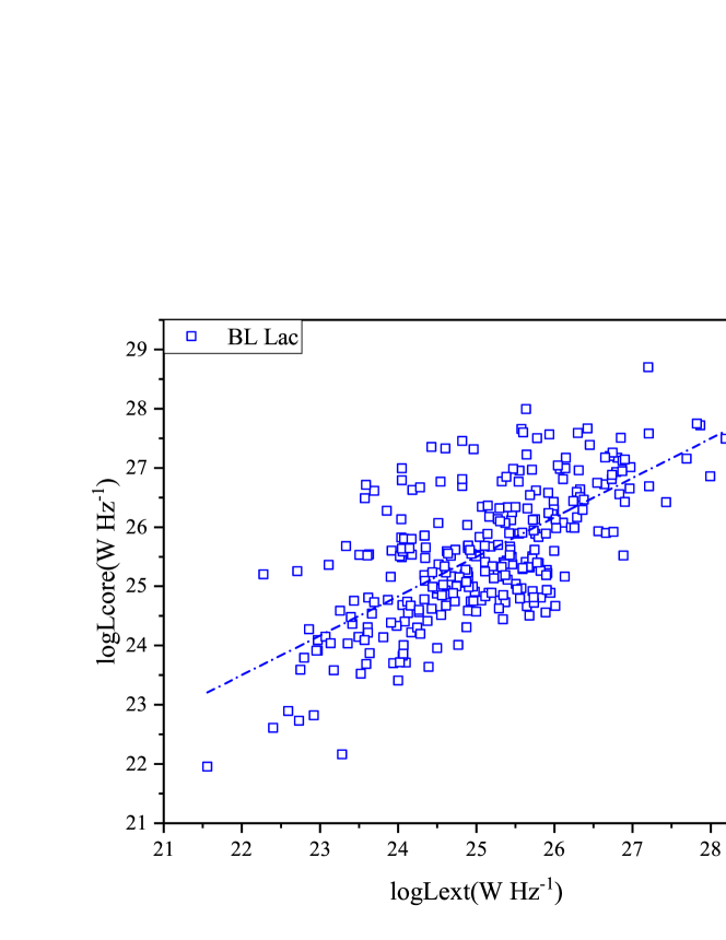
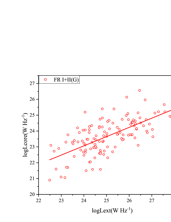
Figure 6: Distributions of core and extended luminosity: 6 for BL Lacs, the broken-dotted line represents the best linear regression between core and extended luminosity for BL Lacs. 6 for FR I/II(G)s, the solid line represents the best linear regression between core and extended luminosity for FR I/II(G)s.

3.3 Doppler Factor

In the unified model, FR I/II(G)s are the parent population of BL Lacs. It means that BL Lacs are the FR radio galaxies with the jets pointing to the observers and boosted. As mentioned in §3.1, one can get an expression for a Doppler factor based on the slope k (0.58), intercept b (9.08) for the linear correlation of FR I/II(G)s,

$$\log\delta=(\log L_{\rm{BL,core}}^{\rm{ob}}-0.58\log L_{\rm{BL,ext}}-9.08)/q$$ (6)

When radio core spectral index $\alpha_{c}=0.0$ (Donate et al., 2001; Abdo et al., 2010; Fan et al., 2016) is adopted, Doppler factors are obtained in a range from $\delta=0.62$ to 113.08 with an average of 15.03 for $q=2$, and from $\delta=0.73$ to 23.38 with an average of 5.43 for $q=3$, which are listed in Col. 2-3 in Table 3.3. The Doppler factors from different literatures for BL Lacs are also presented in Table 3.3.

In addition, based on the unification of BL Lacs and FR I/II(G)s, we propose another method about the core to extended emission ratio of FR I/II(G)s to estimate Doppler factor. The core to extended emission ratio is also called as core-dominance parameter (R), using the expression, $R=S_{\rm{core}}/S_{\rm{ext}}$, or $R=L_{\rm{core}}/L_{\rm{ext}}$. If the core emission is strongly boosted by beaming effect, a close relation between the core-dominance parameter (R) and Doppler factor ($\delta$) should be expected, which have been proposed by Ghisellini et al. (1993): $R=f\delta^{q}$, where the $f=S^{\rm{in}}_{\rm{core}}/S_{\rm{ext}}$, $q=2+\alpha_{c}$ or $3+\alpha_{c}$ (see above). When an unification of BL Lacs, FR Is and FR II(G)s is considered, the intrinsic core to extended emission ratio ($f_{\rm{BL}}$) of BL Lacs should behave as the same as those ($R_{\rm{FR}}$) of FR I/II(G)s, then a Doppler factor can be estimated from following correlation.

$$\delta^{q}=R_{\rm{BL}}/R_{\rm{FR}}$$ (7)

where $R_{\rm{FR}}$ is the core-dominance parameter ($R_{\rm{FR}}=L_{\rm{FR,core}}/L_{\rm{FR,ext}}$) for the FR I/II(G)s, and $R_{\rm{BL}}$ is the observed core-dominance parameter ($R_{\rm{BL}}=L_{\rm{BL,core}}^{\rm{ob}}/L_{\rm{BL,ext}}$) for the BL Lacs. The density distributions of logarithm of core-dominance parameter of BL Lacs and FR I/II(G)s are shown in Figure 7. For the present FR I/II(G)s sample, they shows a peak at log $R_{\rm{FR}}$ = -1.48 in Figure 7. When we used this value to estimate the Doppler factors for the case of $q=2+\alpha_{c}$ and $3+\alpha_{c}$, the Doppler factor values are listed in Col. 4 and Col. 5 in Table 3.3.

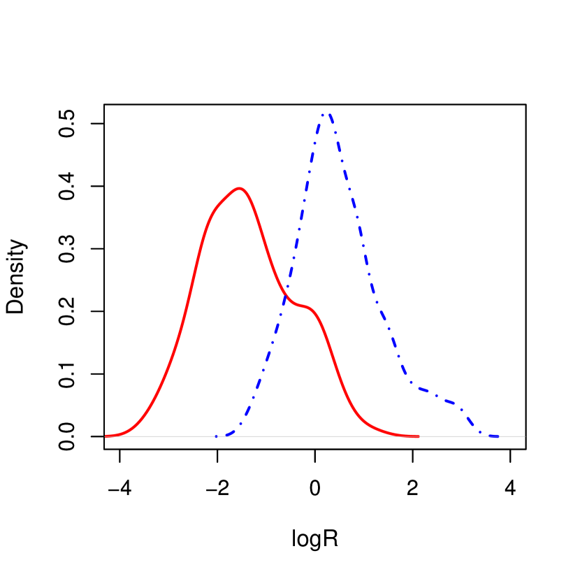
Figure 7: The density distributions of logarithm of core-dominance parameter of BL Lacs and FR I/II(G)s. The broken-dotted line represents BL Lacs and the solid line represents FR I/II(G)s.

$\delta$ from methods and different literatures for BL Lacs q=2 q=3 q=2 q=3 G93 H09 L18 Z20 (1) (2) (3) (4) (5) (6) (7) (8) (9) Min 0.62 0.73 1.15 1.10 0.01 1.1 0.22 0.35 Max 113.08 23.38 201.01 34.32 14.3 24 60.36 53.57 Medium 8.25 4.08 8.24 5.93 2.1 6.3 9.78 7.09 Mean 15.03 5.43 18.23 4.08 3.85 7.9 13.03 10.32 The Doppler factor estimation by the core to extended fitting/regression method.

The Doppler factor estimation by the core to extended flux ratio method. Note: Col. 1 is parameters of samples, Col. 2 Doppler factor at q = 2 by fitting/regression method, Col. 3 Doppler factor at q = 3 by fitting/regression method, Col. 4 Doppler factor at q = 2 by ratio method, Col. 5 Doppler factor at q = 3 by ratio method, Col. 6 Doppler factor by Ghisellini et al. (1993), Col. 7 Doppler factor by Hovatta et al. (2009), Col. 8 Doppler factor by Liodakis et al. (2018), Col. 9 Doppler factor by Zhang et al. (2020).

From different assumptions and methods, it can be found that some Doppler factors for BL Lacs are smaller than unity, which may be caused by the systematic error or the limitation of the methods. For examples, there are 8 BL Lacs in Ghisellini et al. (1993), 5 BL Lacs in Liodakis et al. (2018), and 3 BL Lacs in Zhang et al. (2020) with Doppler factor $\delta<1$. Liodakis et al. (2018) adopted a definite intrinsic brightness temperature to estimate the Doppler factor for BL Lacs. If some BL Lacs was in a low state when it was observed, it is possible to obtain a low observed brightness temperature, then to derive a Doppler factor $\delta<1$ from the limitation of the methods. In our sample, the source 1440+356 with Doppler factor $\delta<1$ in fitting/regression method may also be due to our systematic error or the limitation of our method that the unification of BL Lacs and FR I/II(G)s.

4 Discussions

BL Lacs show special observation properties, such as variability, high and variable polarization, high luminosity, high energetic $\gamma$-ray emissions, or superluminal motion etc. Their special observation properties are due to the beaming effect. When their jets are perpendicular to the line of sight, they are radio galaxies, and FR Is and FR II(G)s are proposed to be the parent population of BL Lacs (Xie et al., 1993; Owen et al., 1996; Fan et al., 1997).

From the available extended luminosities of BL Lacs and FR I/II(G)s, we can see that the probabilities from WRS test and K-S test render discrepant results, p = 0.779 for WRS test and p = 0.326 for K-S test. These results suggest, for the case of the extended luminosity, that BL Lacs are unified with FR I/II(G)s. But there is also a different probability by the WRS test and K-S test, which may be due to the difference in extended luminosity distributions of BL Lacs and FR I/II(G)s. The extended luminosity distribution of BL Lacs is similar to a normal distribution, but that of FR I/II(G)s is marginally different to normal distribution, in particular from $\log L_{\rm{ext}}=25$ to 26 shown in Fig. 8. The asymptotic relative efficiency of the WRS test compared to the t-test is 0.955 for normal distributions,

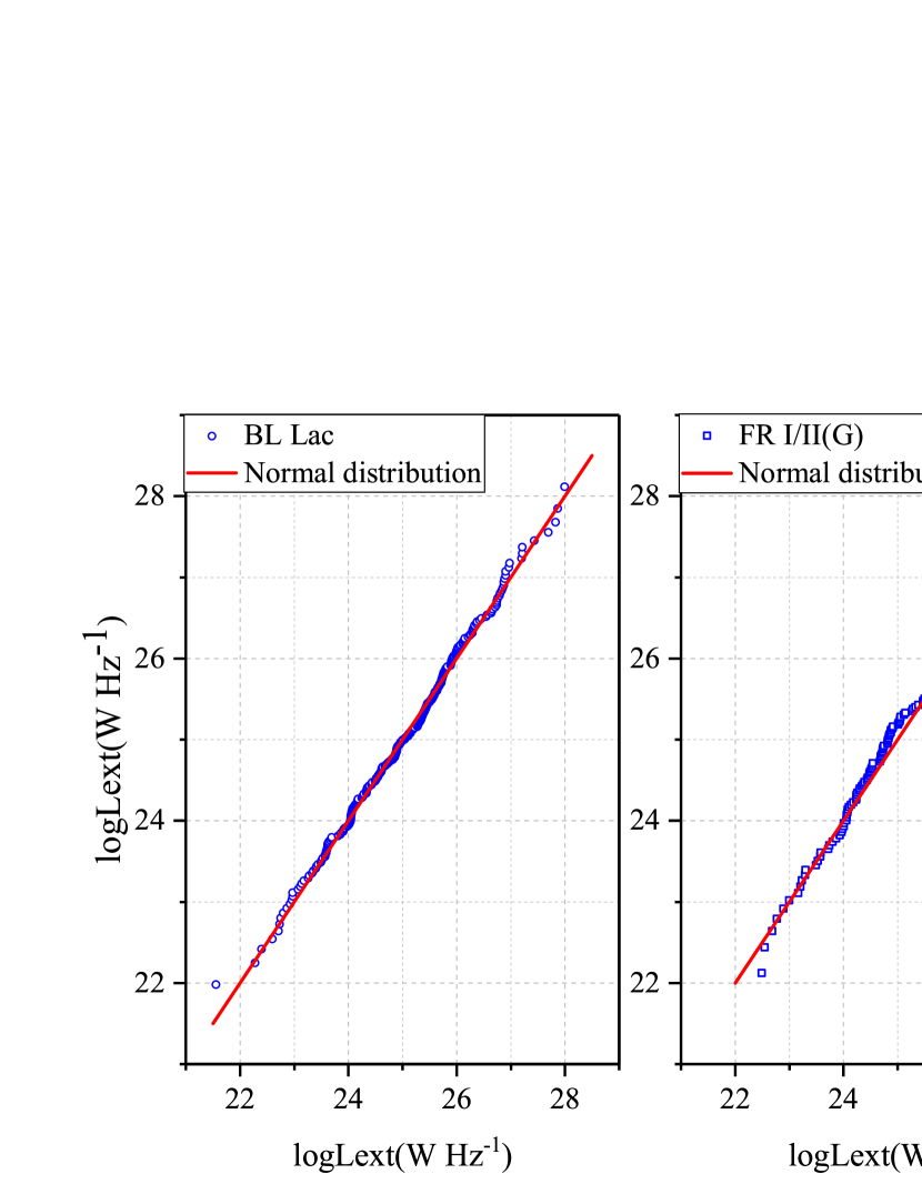
Figure 8: The left panel is the comparison between the extended luminosity distribution of BL Lacs and normal distribution, in which the solid line represents normal distribution and the circular represents BL Lacs. The right panel is the comparison between the extended luminosity distribution of FR I/II(G)s and normal distribution, in which the solid line represents normal distribution and the square represents FR I/II(G)s.

indicating that it can be effectively used for both normal and nonnormal situations (Feigelson & Babu, 2012), while K-S test is not. So the marginal difference of extended luminosity distributions between BL Lacs and FR I/II(G)s is represented in probability that the p value (0.779) for WRS test is higher than that (0.326) of K-S test.

However, the averaged value of the core luminosity of BL Lacs is higher than that of FR I/II(G)s, both WRS test and K-S test suggest that the probabilities for the distribution of the logarithm of the core luminosities of FR I/II(G)s and that of BL Lacs to come from the same parent distribution are very low, they are both $p<10^{-4}$. The clear difference is from the fact that the core luminosities of BL Lacs are strongly beamed.

As mentioned in §1, many methods were proposed to estimate the Doppler factors (Ghisellini et al., 1993; Mattox et al., 1993; Lähteemäki & Valtaoja, 1999; Fan et al., 2013; Chen, 2018; Liodakis et al., 2018; Zhang et al., 2020). In the present work, based on the unified scheme of BL Lacs and FR I/II(G)s, the Doppler factor of BL Lacs is estimated. For BL Lacs objects, the radio band spectrum is flat. For example, Fan et al. (2006) obtained the radio average value of radio spectral index to be $0.235$ for X-ray selected BL Lacs, and 0.044 for radio selected BL Lacs. Pei et al. (2016) studied a samples of 1335 blazars and showed the average radio spectral index, $<\alpha_{\rm{radio}}>$ = $0.02\pm 0.31$ for Fermi-detected BL Lacs, $0.34\pm 0.37$ for non-Fermi-detected BL Lacs. $-0.5\leq\alpha\leq 0.5$ was adopted for BL Lacs in Yuan (2014). $\alpha_{c}$ = 0.0 was also adopted for BL Lacs by Donate et al. (2001); Abdo et al. (2010), and Fan et al. (2016). We adopted the radio core spectral index $\alpha_{c}$ = 0.0 for the radio spectral index. By comparing the Doppler factor between $\alpha_{c}=0$ and $\alpha_{c}=\pm 0.5$, we can find that the Doppler factor for the case $\alpha_{c}=\pm 0.5$ could be several times different from that of $\alpha_{c}=0$ for $q=2$. But for $q=3$, there is marginal difference between $\alpha_{c}=\pm 0.5$ and $\alpha_{c}=0$ to estimate the Doppler factor. The Doppler factor corresponding $\alpha_{c}=0$ or $\pm 0.5$ are listed in Col. 10-15 in Table 1.

The coefficients of regression lines have some degrees of errors as shown in Equations (4) and (5). When we estimated the Doppler factor using the fitting/regression method, the coefficient errors of regression lines do have a great influence, even on the order of magnitude, on the Doppler factor value, but the average fitting/regression should be representative of the true Doppler factor values.

Following the case of the spherical jet (q = 3)(Ghisellini et al., 1993; Xie et al., 1993; Hovatta et al., 2009; Liodakis et al., 2018) and the radio core spectral index as 0 (Donate et al., 2001; Abdo et al., 2010; Fan et al., 2016), we can also compare our Doppler factor estimation results ($\delta_{\rm{TW}}$) with those ($\delta_{\rm{G}}$ by Ghisellini et al. (1993), $\delta_{\rm{H}}$ by Hovatta et al. (2009), $\delta_{\rm{L}}$ by Liodakis et al. (2018), $\delta_{\rm{Z}}$ by Zhang et al. (2020)) from the literatures for the common sources. There are 29 sources in common with Ghisellini et al. (1993), we performed a linear regression and obtained $\delta_{\rm{TW}}=(0.78\pm 0.13)\delta_{\rm{G}}+4.84\pm 0.75$, with a Spearman’s rank correlation coefficient of $r=0.541$ and a chance probability of $p=2.4\times 10^{-3}$, see the upper-left panel in Figure 9. We also performed the regression for the common sources with Hovatta et al. (2009) $\delta_{\rm{TW}}=(0.70\pm 0.13)\delta_{\rm{H}}+4.39\pm 1.10$, Liodakis et al. (2018) $\delta_{\rm{TW}}=(0.17\pm 0.05)\delta_{\rm{L}}+4.88\pm 0.67$ and Zhang et al. (2020) $\delta_{\rm{TW}}=(0.41\pm 0.09)\delta_{\rm{Z}}+3.86\pm 1.27$. The Spearman’s rank correlation coefficients and chance probabilities are $r=0.656$ and $p=3\times 10^{-3}$ for 18 sources with Hovatta et al. (2009); $r=0.537$ and $p=3\times 10^{-4}$ for 41 sources with Liodakis et al. (2018), and $r=0.537$ and $p=0.016$ for 20 sources with Zhang et al. (2020). The best fitting results are all shown in Figure 9. The correlation coefficients for our Doppler factor estimation results with other literatures for common sources are both larger than 0.5 with probabilities $<0.05$, indicating that our Doppler factor estimation by fitting/regression method is correlated with other samples.

Figure 9: Plot of the correlation for common sources between our Doppler factor ($\delta_{\rm{TW}}$) by the fitting/regression method and those from Ghisellini et al. (1993), $\delta_{\rm{G}}$, Hovatta et al. (2009), $\delta_{\rm{H}}$, Liodakis et al. (2018), $\delta_{\rm{L}}$, Zhang et al. (2020), $\delta_{\rm{Z}}$.

We also compare the correlations for common sources with other Doppler factor ($\delta_{G}$, $\delta_{H}$, $\delta_{L}$, $\delta_{Z}$) for Doppler factor (q=3) estimation of the core to extended flux ratio method as do the core to extended luminosity fitting/regression method. The Spearman’s rank correlation coefficients between the ratio method and those samples are $r=0.347$ and $p=0.07$ for Ghisellini et al. (1993), $r=0.411$, $p=0.09$ for Hovatta et al. (2009), $r=0.182$, $p=0.254$ for Liodakis et al. (2018), and $r=0.513$, $p=0.022$ for Zhang et al. (2020). A detailed comparison between the ratio method and fitting/regression method is listed in Table 4. From Table 4, a comparison of the distributions of the core to extended flux ratio is straightforward, but the correlation coefficients of this ratio method are less relevant and less convincing than those of fitting/regression method as mentioned above.

A comparison between the fitting/regression method and the ratio method. samples $r_{f}$ $p_{f}$ $r_{r}$ $p_{r}$ (1) (2) (3) (4) (5) G93 0.541 $2.4\times 10^{-3}$ 0.347 0.07 H09 0.656 $3\times 10^{-3}$ 0.411 0.09 L18 0.537 $3\times 10^{-4}$ 0.182 0.254 Z20 0.537 0.016 0.513 0.022 The correlation coefficients and probabilities for fitting/regression method.

The correlation coefficients and probabilities for ratio method. Note: Col. 1 are samples, Col. 2 the correlation coefficients for fitting/regression method, Col. 3 the probabilities for fitting/regression method, Col. 4 the correlation coefficients for ratio method, Col. 5 the probabilities for ratio method.

5 Conclusions

In this work, we compiled the core and extend flux densities for a sample of BL Lacs, FR Is and FR II(G)s, and calculated their corresponding luminosities. We used WRS test and K-S test to analyze the cumulative distribution for extended luminosity, $L_{\rm{ext}}$, of BL Lacs and that of FR I/II(G)s, and found that the probabilities for the both to be from the same distribution are $p_{\rm{WRS}}=0.779$ and $p_{\rm{K-S}}=0.326$. Based on the unification of BL Lacs and FR I/II(G)s, we proposed a core to extended luminosities fitting/regression method and a ratio method of core to extended emissions to estimate the Doppler factor for BL Lacs, and compared our results with those in the literatures. Our conclusions are as follows:

1. From the extended radio luminosities, BL Lacs are unified with FR I and FR II(G) radio galaxies, which confirmed the results by Xie et al. (1993), Owen et al. (1996), Fan et al. (1997).

2. Our Doppler factors from the fitting/regression method is correlated with those by Ghisellini et al. (1993), Hovatta et al. (2009), Liodakis et al. (2018), and Zhang et al. (2020).

3. The Doppler factors of BL Lacs estimated by the fitting/regression method is in a range of from $\delta$ = 0.73 to $\delta$ = 23.38 for the case of q = 3, $\alpha_{c}=0$. The work is supported by the National Natural Science Foundation of China (NSFC U2031201, NSFC 11733001, NSFC U1938110, NSFC U1531245), Natural Science Foundation of Guangdong Province (2019B030302001), Guangzhou University (NO YM2020001, No 2019GDJC-D18), and supports for Astrophysics Key Subjects of Guangdong Province and Guangzhou City. We thank the anonymous referee for the comments that made us improve our manuscript.

The complete Table 1 sample.

lcccccccccccccc The core and extended fluxes or luminosities of whole samples and the Doppler factor of BL Lacs. Sourceclass$z$ $S_{\rm{core}}$ $S_{\rm{ext}}$Ref$logL_{\rm{core}}$$logL_{\rm{ext}}$Ref$\delta_{2}$ $\delta_{2}$$\delta_{2}$$\delta_{3}$$\delta_{3}$$\delta_{3}$
Name (mJy)(mJy) (W Hz${}^{-1})$(W Hz${}^{-1})$ ($\alpha_{c}=0$ 0.5-0.5)($\alpha_{c}=0$0.5-0.5)
(1)(2) (3)(4)  (5)(6)(7)(8)(9)(10)(11)(12)(13)(14)(15)
Sourceclass$z$ $S_{\rm{core}}$ $S_{\rm{ext}}$Ref$logL_{\rm{core}}$$logL_{\rm{ext}}$Ref$\delta_{2}$ $\delta_{2}$$\delta_{2}$$\delta_{3}$$\delta_{3}$$\delta_{3}$
Name (mJy)(mJy) (W Hz${}^{-1})$(W Hz${}^{-1})$ ($\alpha_{c}=0$ 0.5-0.5)($\alpha_{c}=0$0.5-0.5)
(1)(2) (3)(4)  (5)(6)(7)(8)(9)(10)(11)(12)(13)(14)(15)
0003+003 B 1.037 480 206 P19 27.17 26.81 18.74 10.43 49.79 7.06 5.34 10.43
0003-066 B 0.347 1850 1504.47 P19 26.73 26.64 12.55 7.57 29.16 5.40 4.24 7.57
0007+124 I 0.156 4 751.02 F11 23.47 25.75
0007+472 B 0.280 67 22 P19 25.17 24.69 7.69 5.11 15.17 3.90 3.21 5.11
0011+1853 B 0.473 140 104 P19 25.89 25.76 8.58 5.58 17.57 4.19 3.42 5.58
0013+790 II(G) 0.840 4.4 1028.6 F11 25.21 27.58
0021+055 B 2.050 28 53 P19 26.56 26.83 9.04 5.82 18.84 4.34 3.52 5.82
0029-271 B 0.333 11 105 P19 24.67 25.65 2.27 1.93 2.98 1.73 1.60 1.93
0032+595 B 0.086 44 5 P19 23.92 22.97 5.71 4.03 10.20 3.19 2.71 4.03
0033+156 B 1.162 125 28 P19 26.96 26.31 20.43 11.18 55.86 7.47 5.61 11.18
0038+328 II(G) 0.482 0.47 1199.53 NED 23.64 27.05
0039+398 I 0.109 1 225 P19 22.52 24.88
0043+008 B 2.149 2 2 P19 25.27 25.27 5.86 4.11 10.55 3.25 2.75 4.11
0044+193 B 0.181 7 17 P19 23.71 24.10 2.13 1.83 2.74 1.65 1.54 1.83
0048-09 B 0.634 887 108.45 F11 26.98 26.07 24.62 12.97 71.62 8.46 6.24 12.97
0052+251 B 0.154 1 1 P19 22.73 22.73 1.71 1.54 2.05 1.43 1.36 1.54
0053+260 I 0.195 23.00 25.04 F11
0055-01 I 0.045 93 2043.47 M93 23.67 25.01
0057+026 B 0.599 99 16 P19 25.83 25.04 13.02 7.80 30.65 5.54 4.34 7.80
0057+3021 I 0.017 23.40 23.58 B11
0059+581 B 0.644 1570 7 P19 27.32 24.96 75.51 31.80 319.16 17.86 11.83 31.80
0104+32 I 0.016 22.04 24.25 Z95
0106+130 II(G) 0.060 38 5140.8 F11 23.53 25.67
0106+729 II(G) 0.181 23.76 26.11 F11
0107+32224 I 0.017 22.80 23.86 B11
0109+224 B 0.265 330 5.44 F11 25.82 24.04 25.12 13.18 73.56 8.58 6.31 13.18
0109+492 II(G) 0.395 3.64 734.59 NED 24.33 26.63
0115-261 I 0.053 18 5 P19 23.10 22.54
0118-272 B 0.559 1137 63 P19 26.97 25.71 30.74 15.49 96.28 9.81 7.08 15.49
0120+340 B 0.272 31 2 P19 24.81 23.62 10.35 6.48 22.55 4.75 3.80 6.48
0121+318 B 0.654 82 89 P19 26.08 26.11 8.42 5.50 17.14 4.14 3.38 5.50
0122+090 B 0.339 1 1 P19 23.52 23.52 2.51 2.09 3.41 1.85 1.69 2.09
0123+3315 I 0.016 20.90 22.49 B11
0125+287 II(G) 0.437 185 105 NED 26.14 25.89
0125-0120 I 0.018 22.80 24.08 B11
0138-097 B 0.733 696 504 P19 26.93 26.79 14.33 8.42 34.82 5.90 4.58 8.42
0140+219B B 0.599 7 13 P19 24.89 25.16 4.07 3.07 6.49 2.55 2.23 3.07
0145+138 B 0.125 2 1 P19 22.89 22.59 2.27 1.92 2.98 1.72 1.60 1.92
0154+286 II(G) 0.735 5.3 536.7 NED 25.13 27.14
0156+0537 I 0.019 21.70 23.29 B11
0158+003 B 0.299 9 1 P19 24.37 23.41 7.14 4.82 13.74 3.71 3.07 4.82
0159+002 B 0.163 7 12 P19 23.70 23.94 2.34 1.98 3.12 1.77 1.63 1.98
0200-0011 B 0.366 30 88 P19 25.04 25.51 3.82 2.92 5.98 2.45 2.15 2.92
0204+29 I 0.110 171 158 P19 24.75 24.71
0208+352 B 0.318 5 1 P19 24.31 23.61 5.85 4.11 10.54 3.25 2.74 4.11
0208-512 B 0.999 233 3169 P19 26.86 27.99 5.91 4.14 10.69 3.27 2.76 4.14
0212+364 B 0.490 82 1 P19 25.54 23.63 23.91 12.67 68.86 8.30 6.13 12.67
0213-132 I 0.147 99 98 P19 24.82 24.82
0214+083 B 1.400 296 166 P19 27.12 26.87 16.94 9.62 43.51 6.60 5.04 9.62
0219+042 I 0.022 161 130 P19 23.30 23.21
0219+428 B 0.444 814 510.84 F11 26.75 26.55 13.67 8.10 32.68 5.72 4.46 8.10
0220+427 I 0.021 22.59 24.69 F11
0221+27 II(G) 0.310 20 884 F11 24.83 26.48
0227+020 B 0.457 9 18 P19 24.76 25.06 3.74 2.87 5.80 2.41 2.12 2.87
0230+344 B 0.458 123 56 P19 25.89 25.55 9.92 6.27 21.31 4.62 3.71 6.27
0232+202 B 0.599 43 7 P19 25.68 24.89 12.06 7.33 27.65 5.26 4.15 7.33
0232+264 B 0.599 554 1 P19 26.79 24.05 76.10 32.00 322.50 17.96 11.89 32.00
0240+1656 B 0.599 40 7 P19 25.65 24.89 11.63 7.12 26.35 5.13 4.06 7.12
0245+269A B 0.599 28 1 P19 25.49 24.05 17.11 9.70 44.09 6.64 5.07 9.70
0247-027 I 0.087 23.45 24.53 Z95
0255+05 I 0.024 22.65 24.74 Z95
0257+342 B 0.245 9 2 P19 24.15 23.49 5.25 3.77 9.12 3.02 2.58 3.77
0300+162 I 0.033 8 1188.74 F11 22.31 24.48
0300+470 B 0.475 1566 62.16 F11 26.95 25.55 33.63 16.65 108.56 10.42 7.45 16.65
0301-243 B 0.260 228 132 F11 25.67 25.43 8.30 5.44 16.81 4.10 3.35 5.44
03020-037 I 0.005 28 102 P19 23.37 23.93
0305+03 I 0.029 964 2436 DM14 24.28 24.68
0307+169 II(G) 0.256 6.04 963.14 F11 24.12 26.32
0308+0406 I 0.029 24.20 24.67 B11
0308+104 B 0.599 886 1 P19 26.99 24.05 96.24 38.61 441.05 21.00 13.59 38.61
0314+063 B 0.599 27 2 P19 25.48 24.35 13.74 8.14 32.91 5.74 4.47 8.14
0315+41 I 0.026 40 3490 P19 22.78 24.72
0317+185 B 0.190 17 15 P19 24.22 24.17 3.65 2.82 5.62 2.37 2.10 2.82
0319+4130 I 0.018 25.40 24.81 B11
0320-37 I 0.006 51 71949 DM14 21.58 24.73
0329+704 B 0.599 37 12 P19 25.53 25.04 9.19 5.90 19.25 4.39 3.55 5.90
0331-001 I 0.139 24.53 26.12 Z95
0350-371 B 0.165 14 2.9 P19 24.04 23.35 5.08 3.67 8.74 2.96 2.53 3.67
0356+102 I 0.030 9 4961 P19 22.31 25.05
036-019 B 0.850 14 2 P19 25.52 24.67 11.59 7.10 26.23 5.12 4.06 7.10
0402-014 B 0.920 876 102 P19 27.39 26.45 30.35 15.34 94.68 9.73 7.03 15.34
0410+110 II(G) 0.306 25.15 26.39 F11
0414+009 B 0.287 24.76 25.30 F11 3.18 2.53 4.68 2.16 1.94 2.53
0414+378 I 0.049 252 230 P19 24.28 24.24
0419+194 B 0.512 8 1 P19 24.77 23.87 8.39 5.48 17.05 4.13 3.37 5.48
0422+004 B 0.310 1465 1.75 F11 26.61 23.69 78.75 32.88 337.52 18.37 12.12 32.88
0430+05 I 0.033 25.19 24.05 Z95
0433+29 II(G) 0.218 108.9 13063.54 F11 25.22 27.29
0449-175 I 0.031 21.58 24.38 Z95
0453+22 II(G) 0.214 4.1 937.86 F11 23.77 26.13
0454+844 B 1.340 392 1346.15 F11 27.16 27.69 10.17 6.40 22.03 4.69 3.76 6.40
0502+675 B 0.314 17 4 P19 24.68 24.05 6.69 4.58 12.61 3.55 2.96 4.58
0521-365 B 0.055 3124 5213.24 F11 25.41 25.63 5.39 3.85 9.46 3.08 2.62 3.85
0545-199 I 0.053 23.23 24.00 Z95
0548-322 B 0.069 80 92.73 F11 24.01 24.07 3.04 2.43 4.40 2.10 1.89 2.43
0605+48 II(G) 0.277 0.5 996.1 F11 23.10 26.40
0607+710 B 0.267 12 11 P19 24.41 24.38 3.96 3.01 6.27 2.50 2.20 3.01
0620-52 I 0.051 260 946.39 M93 24.25 24.81
0625-35 I 0.055 600 1650 DM14 24.67 25.11
0634-205 I 0.055 22.74 24.90 Z95
0647+250 B 0.203 42 36 P19 24.68 24.61 4.59 3.38 7.62 2.76 2.39 3.38
0648-165 B 0.599 2120 4 P19 27.33 24.60 97.49 39.01 448.70 21.18 13.69 39.01
0651+542 II(G) 0.238 2 963.2 F11 23.57 26.25
0702+749 II(G) 0.292 9.64 631.90 F11 24.46 26.28
0704+384 B 0.579 61 260 P19 25.93 26.56 5.28 3.79 9.20 3.03 2.59 3.79
0708+7413 B 0.371 65 151 P19 25.32 25.68 4.69 3.44 7.84 2.80 2.42 3.44
0716+714 B 0.300 2460 88.04 K05 26.77 25.33 31.75 15.90 100.55 10.03 7.21 15.90
0722+30 I 0.019 22.90 22.89 Z95
0723-008 B 0.128 24.89 25.95 F11 2.40 2.01 3.21 1.79 1.65 2.01
0734+805 II(G) 0.118 7 1271.2 F11 23.44 25.70
0735+178 B 0.424 1919 59.39 K10 26.98 25.47 36.63 17.83 121.67 11.03 7.83 17.83
0737+746 B 0.315 21 1 P19 24.76 23.43 11.02 6.82 24.53 4.95 3.94 6.82
0738+5451 B 0.720 279 1 P19 26.63 24.18 57.64 25.62 222.65 14.92 10.14 25.62
0742+333 B 0.611 124 1 P19 26.13 24.04 35.92 17.55 118.53 10.89 7.74 17.55
0743+7458 B 0.607 22 11 P19 25.41 25.11 7.65 5.09 15.08 3.88 3.20 5.09
0744+55 I 0.036 105 1596 P19 23.84 25.02
0749+540 B 0.200 737 133.98 F11 25.89 25.15 12.90 7.74 30.26 5.50 4.31 7.74
0754+100 B 0.266 1087 57.73 F11 26.35 25.07 23.04 12.30 65.56 8.10 6.01 12.30
0759+508 B 0.054 8 10 P19 22.82 22.92 1.68 1.51 2.00 1.41 1.34 1.51
0800+244 I 0.040 4 135 P19 22.48 24.00
0806+505 B 1.207 12 11 P19 25.83 25.79 7.87 5.21 15.65 3.96 3.25 5.21
0806+524 B 0.138 66 70.8 P19 24.52 24.55 3.98 3.02 6.31 2.51 2.20 3.02
0808+019 B 1.148 424 11.16 F11 27.22 25.64 43.14 20.32 151.29 12.30 8.59 20.32
0810+5619 B 0.510 49 1 P19 25.61 23.92 21.25 11.53 58.86 7.67 5.73 11.53
0812+578 B 0.054 46 18 P19 23.58 23.17 3.39 2.66 5.10 2.26 2.01 2.66
0812+6217 B 0.599 20 18 P19 25.43 25.39 6.52 4.48 12.18 3.49 2.92 4.48
0818-128 B 0.074 270 540 F11 24.59 24.89 3.44 2.69 5.20 2.28 2.03 2.69
0819+525 B 0.599 23 20 P19 25.41 25.35 6.50 4.47 12.14 3.48 2.92 4.47
0820+225 B 0.951 26.42 27.43 F11 5.19 3.73 8.99 3.00 2.56 3.73
0824+294 II(G) 0.458 116.1 636.9 F11 25.97 26.71
0824+4204 B 0.223 7 40 P19 24.01 24.77 1.92 1.68 2.38 1.54 1.45 1.68
0826+180 B 0.089 23.96 24.50 F11 2.16 1.85 2.80 1.67 1.55 1.85
0828+493 B 0.548 25.90 26.66 F11 4.77 3.49 8.03 2.83 2.44 3.49
0829+046 B 0.174 643 103.90 F11 25.69 24.90 12.13 7.37 27.88 5.28 4.16 7.37
0837-12 B 0.198 160 672 F11 25.28 25.90 3.87 2.95 6.07 2.46 2.17 2.95
0847+548 B 0.367 6 47 P19 24.45 25.34 2.16 1.85 2.79 1.67 1.55 1.85
0850+443 B 0.382 31 46 P19 25.17 25.34 4.96 3.60 8.45 2.91 2.50 3.60
0850+625 B 0.267 224 1 P19 25.68 23.33 34.26 16.90 111.26 10.55 7.53 16.90
0851+203 B 0.306 1719 7 P19 26.67 24.28 56.72 25.29 217.92 14.76 10.05 25.29
0855+082 B 0.455 32 82 P19 25.39 25.80 4.72 3.46 7.91 2.81 2.43 3.46
0905-097 B 0.053 23.69 23.59 F11 2.91 2.35 4.15 2.04 1.84 2.35
0906+041 B 3.200 78 33 P19 27.58 27.21 22.94 12.26 65.18 8.07 5.99 12.26
0908+445 B 0.298 31 126 P19 24.97 25.58 3.36 2.64 5.04 2.24 2.00 2.64
0912+297 B 0.101 222 79.23 F11 24.78 24.33 6.22 4.32 11.44 3.38 2.84 4.32
0915+32 I 0.062 23.12 24.06 Z95
0915-118 I 0.065 24.51 26.51 Z95
0917+45 II(G) 0.174 44 1873 F11 24.64 26.27
0922+3625 B 1.015 167 1 P19 26.77 24.54 53.16 24.01 199.87 14.14 9.68 24.01
0923+750 B 0.638 5 52 P19 24.81 25.83 2.37 2.00 3.16 1.78 1.64 2.00
0925+504 B 0.370 462 615.03 F11 26.16 26.29 8.29 5.43 16.77 4.10 3.35 5.43
0926+2550 B 0.539 113 8 P19 26.04 24.89 18.25 10.21 48.04 6.93 5.26 10.21
0927+352 B 0.435 394 47 F11 26.33 25.41 18.12 10.15 47.59 6.90 5.24 10.15
0927+500 B 0.187 15 7 P19 24.14 23.81 4.22 3.17 6.83 2.61 2.28 3.17
0944+734 I 0.058 131 129 P19 24.06 24.06
0945+222 B 0.716 48 79 P19 26.00 26.21 7.18 4.84 13.86 3.72 3.09 4.84
0945+664 B 0.850 1407 33 P19 27.57 25.94 52.64 23.82 197.26 14.05 9.63 23.82
0946+003 B 0.585 108 3 P19 26.07 24.51 24.31 12.84 70.41 8.39 6.19 12.84
0950+495 B 0.380 4 1 P19 24.22 23.61 5.25 3.77 9.12 3.02 2.58 3.77
0951+216 B 0.296 33 303 P19 24.94 25.90 2.62 2.16 3.61 1.90 1.73 2.16
0952+226A B 1.211 17 117 P19 25.92 26.76 4.57 3.37 7.59 2.75 2.38 3.37
0954+65 B 0.368 637 746.53 F11 26.29 26.36 9.15 5.88 19.14 4.37 3.54 5.88
0958+290 II(G) 0.185 34.46 1238.36 F11 24.57 26.13
0958+294 B 0.558 142 30 P19 26.12 25.45 13.84 8.18 33.23 5.76 4.49 8.18
0958+426A B 0.664 23 37 P19 25.51 25.71 5.71 4.03 10.21 3.20 2.71 4.03
1003+328 B 1.026 58 173 P19 26.43 26.90 7.44 4.98 14.53 3.81 3.15 4.98
1003+351 II(G) 0.101 900 772 F11 25.40 25.33
1009+427 B 0.365 29 17 P19 25.09 24.86 6.26 4.34 11.53 3.40 2.85 4.34
1011+446 B 0.796 7 15 P19 25.33 25.66 4.83 3.53 8.17 2.86 2.46 3.53
1011+496 B 0.212 24.91 24.98 F11 4.69 3.44 7.84 2.80 2.42 3.44
1015+383 B 0.387 16 101 P19 24.92 25.72 2.89 2.34 4.12 2.03 1.83 2.34
1020+493 B 0.390 12 52 P19 24.73 25.37 2.95 2.37 4.22 2.06 1.85 2.37
1027+555A B 0.435 7 73 P19 24.72 25.74 2.27 1.93 2.98 1.73 1.60 1.93
1028+511 B 0.360 23 11 P19 24.93 24.61 6.14 4.27 11.23 3.35 2.82 4.27
1030+585 II(G) 0.428 1.38 837.37 NED 23.99 26.78
1034+5727 B 0.830 89 37 P19 26.13 25.75 11.44 7.03 25.78 5.08 4.03 7.03
1040+31 I 0.036 23.48 24.14 Z95
1044+549 B 0.540 4 2 P19 24.57 24.27 5.08 3.67 8.74 2.96 2.53 3.67
1055+0519 B 0.890 179 25 P19 26.62 25.76 19.85 10.92 53.75 7.33 5.52 10.92
1055+567 B 0.143 178 69 P19 24.98 24.57 6.68 4.57 12.58 3.55 2.96 4.57
1101+384 B 0.030 520 156.65 F11 24.09 23.57 4.68 3.44 7.83 2.80 2.42 3.44
1101+411 B 0.035 13 8 P19 22.61 22.40 1.86 1.64 2.28 1.51 1.42 1.64
1106+244 B 0.482 18 1 P19 25.16 23.90 12.81 7.69 29.96 5.47 4.29 7.69
1116+227 B 0.422 104 34 P19 25.67 25.18 9.81 6.21 20.99 4.58 3.69 6.21
1118+424 B 0.124 19 11 P19 23.87 23.64 3.49 2.72 5.28 2.30 2.04 2.72
1122+39 I 0.007 21.06 23.16 Z95
1133+704 B 0.045 131 220.48 F11 23.83 24.06 2.50 2.08 3.40 1.84 1.69 2.08
1142+198 I 0.022 250 2107.56 F11 23.52 24.44
1144+352 B 0.063 537 126 F11 24.74 24.12 6.90 4.69 13.14 3.63 3.02 4.69
1144-379 B 1.048 2182 18 P19 27.66 25.58 74.60 31.49 314.06 17.72 11.75 31.49
1145+1936 I 0.021 23.30 24.36 B11
1147+245 B 0.200 664 20 F11 25.86 24.33 21.41 11.60 59.46 7.71 5.76 11.60
1148+592 B 0.118 95 36 P19 24.55 24.13 5.47 3.89 9.63 3.10 2.64 3.89
1150+449A B 0.599 9 5 P19 25.00 24.74 6.08 4.24 11.10 3.33 2.81 4.24
1151+6039 B 1.120 75 1 P19 26.69 24.82 40.68 19.39 139.89 11.83 8.31 19.39
1154+435 B 0.230 93 13 P19 25.19 24.33 9.94 6.28 21.37 4.62 3.71 6.28
1202+492 B 0.452 40 71 P19 25.47 25.72 5.45 3.88 9.58 3.10 2.63 3.88
1203+238 B 0.599 8 30 P19 24.95 25.52 3.41 2.67 5.13 2.27 2.02 2.67
1203+645 II(G) 0.372 730 579 F11 26.56 26.46
1208+322 B 0.389 7 149 P19 24.56 25.89 1.71 1.53 2.04 1.43 1.36 1.53
1210+121 B 0.369 170 81.97 F11 25.91 25.59 9.83 6.22 21.05 4.59 3.69 6.22
1215+303 B 0.130 355 157.77 F11 25.21 24.85 7.17 4.83 13.82 3.72 3.08 4.83
1216+06 I 0.006 22.68 23.98 Z95
1217+348 B 0.643 258 94 P19 26.43 25.99 13.71 8.12 32.81 5.73 4.46 8.12
1218+285 B 0.102 1118 10.52 P19 25.53 23.50 25.63 13.40 75.58 8.69 6.38 13.40
1218+460 B 0.525 30 37 P19 25.37 25.46 5.78 4.07 10.36 3.22 2.72 4.07
1220+337C B 0.599 459 383 P19 26.81 26.73 12.98 7.78 30.52 5.52 4.33 7.78
1220+373 B 0.491 15 138 P19 25.17 26.13 2.92 2.36 4.17 2.04 1.84 2.36
1221+245 B 0.218 179 25 P19 25.37 24.52 10.86 6.74 24.06 4.91 3.91 6.74
1221+809 B 0.369 447 71 F11 26.25 25.46 16.04 9.21 40.45 6.36 4.88 9.21
1222+13 I 0.003 21.72 23.23 F11
1222+488 B 0.647 20 18 P19 25.50 25.45 6.73 4.60 12.70 3.56 2.97 4.60
1227+255 B 0.135 351 1 P19 25.26 22.71 31.76 15.90 100.57 10.03 7.21 15.90
1228+12 I 0.004 3097 68469 DM14 23.34 24.69
1229.2+6430 B 0.163 42.49 3.48 F11 24.48 23.39 8.25 5.41 16.67 4.08 3.34 5.41
1229+290 B 0.236 60 54 P19 25.00 24.95 5.28 3.79 9.21 3.03 2.59 3.79
1229+405 B 0.638 52 57 P19 25.98 26.02 8.03 5.29 16.08 4.01 3.29 5.29
1235+632 B 0.297 22 21 P19 24.74 24.72 4.60 3.39 7.64 2.76 2.39 3.39
1238+414 B 0.499 10 19 P19 24.84 25.11 3.93 2.99 6.21 2.49 2.19 2.99
1239+069 B 0.150 10 1 P19 23.80 22.80 5.59 3.96 9.91 3.15 2.67 3.96
1243+4402 B 1.152 43 5 P19 26.33 25.40 18.25 10.21 48.05 6.93 5.26 10.21
1246+586 B 0.847 278 136 F11 26.64 26.33 13.94 8.23 33.56 5.79 4.51 8.23
1247+443 B 1.812 12 4 P19 25.90 25.42 10.88 6.75 24.11 4.91 3.91 6.75
1250+532 B 0.369 346 50 F11 26.34 25.50 17.19 9.73 44.37 6.66 5.08 9.73
1251+278 II(G) 0.086 22.99 25.38 F11
1251-12 I 0.014 22.87 24.30 Z95
1254+476 II(G) 0.996 1.6 1352.96 F11 24.92 27.85
1255+244 B 0.141 7 1 P19 23.60 22.75 4.57 3.37 7.59 2.75 2.38 3.37
1259+2757 I 0.024 21.10 22.99 B11
1259+4112 B 0.649 19 14 P19 25.34 25.21 6.60 4.53 12.38 3.52 2.94 4.53
1302+715 B 0.599 31 1 P19 25.51 24.02 17.80 10.01 46.47 6.82 5.18 10.01
1308+27 II(G) 0.240 2.79 472.09 F11 23.74 25.97
1309-216 B 1.491 140 45 F11 27.20 26.71 20.66 11.27 56.69 7.53 5.64 11.27
1310+560 B 0.975 235 33 P19 26.99 26.14 23.74 12.60 68.22 8.26 6.11 12.60
1312+240 B 2.145 101 31 P19 27.26 26.74 21.51 11.65 59.83 7.74 5.77 11.65
1318-43 I 0.011 23.48 24.18 Z95
1319+428 II(G) 0.079 22.69 25.27 F11
1322+36 I 0.018 23.29 23.49 Z95
1324+478 B 0.683 15 30 P19 25.29 25.59 4.83 3.52 8.16 2.86 2.46 3.52
1328+506 B 0.599 19 3 P19 25.24 24.44 9.83 6.22 21.05 4.59 3.69 6.22
1338+3851 I 0.246 24.70 26.19 B11
1339+554 B 0.207 30 4 P19 24.54 23.66 7.37 4.94 14.33 3.79 3.13 4.94
1343-60 I 0.013 2730 3850 DM14 24.09 24.24
1345+735 B 0.290 17 372 P19 24.67 26.01 1.79 1.59 2.17 1.47 1.39 1.59
1346+26 I 0.063 23.95 24.91 Z95
1350+4922 B 0.397 63 61 P19 25.38 25.36 6.21 4.31 11.43 3.38 2.84 4.31
1356+393 B 0.800 63 31 P19 26.30 25.99 11.81 7.21 26.90 5.19 4.10 7.21
1400+162 B 0.244 233 311.19 F11 25.62 25.75 6.36 4.39 11.79 3.43 2.88 4.39
1402+042 B 0.344 21 12 P19 24.86 24.62 5.64 3.99 10.04 3.17 2.69 3.99
1404+286 B 0.077 991 1909 P19 25.11 25.40 4.48 3.32 7.38 2.72 2.36 3.32
1407+595 B 0.496 17 3 P19 25.09 24.34 8.88 5.74 18.39 4.29 3.48 5.74
1409+524 II(G) 0.464 10 7364 NED 24.93 27.80
1413+135 B 0.247 1080 4.091 K10 26.27 23.85 47.86 22.08 173.76 13.18 9.12 22.08
1414+110 I 0.025 56 1649.57 F11 22.96 24.43
1414+375 B 0.920 41 4 P19 26.17 25.16 17.78 10.00 46.39 6.81 5.18 10.00
1418+546 B 0.153 1058 19.82 F11 25.80 24.08 23.98 12.70 69.14 8.31 6.14 12.70
1420+198 II(G) 0.270 6.2 894.32 F11 24.16 26.32
1421+582 B 0.635 6 89 P19 24.51 25.68 1.85 1.64 2.27 1.51 1.42 1.64
1422+026 I 0.037 662 1868 P19 24.60 25.05
1424+240 B 0.160 250 60 P19 25.23 24.61 8.68 5.64 17.85 4.23 3.44 5.64
1426+340 B 1.553 23 5 P19 26.32 25.65 15.08 8.76 37.26 6.10 4.71 8.76
1426+428 B 0.129 19.1 2.1 P19 23.91 22.95 5.75 4.05 10.30 3.21 2.72 4.05
1435+174A B 0.599 355 174 P19 26.60 26.29 13.65 8.09 32.61 5.71 4.45 8.09
1437+397 B 0.344 38 24 P19 25.06 24.86 6.03 4.21 10.98 3.31 2.79 4.21
1440+122 B 0.163 17.2 1.3 P19 24.09 22.97 6.99 4.74 13.37 3.66 3.04 4.74
1440+356 B 0.079 1 13 P19 22.17 23.28 0.62 0.68 0.53 0.73 0.76 0.68
1441+522 II(G) 0.722 104 938.4 F11 24.74 25.69
1441+536 B 2.454 17 1 P19 26.77 25.54 27.45 14.15 82.80 9.10 6.64 14.15
1443+634 B 0.298 8 7 P19 24.30 24.25 3.81 2.91 5.94 2.44 2.15 2.91
1446+3620 B 1.565 29 1 P19 26.85 25.39 33.28 16.51 107.07 10.35 7.41 16.51
1447+771 II(G) 1.132 6 454 F11 25.67 27.55
1448+634 I 0.042 22.57 24.73 F11
1449+537 B 0.432 6 16 P19 24.57 25.00 3.14 2.50 4.60 2.14 1.92 2.50
1452+516 B 1.083 80 53 P19 26.51 26.33 11.99 7.29 27.44 5.24 4.13 7.29
1454+510 B 0.599 212 20 P19 26.32 25.30 19.27 10.67 51.68 7.19 5.42 10.67
1458+224 B 0.235 60 25 P19 24.88 24.50 6.22 4.32 11.45 3.38 2.84 4.32
1459+551 B 0.339 18 56 P19 24.85 25.34 3.44 2.68 5.18 2.28 2.02 2.68
1501+481 B 0.345 10 46 P19 24.63 25.29 2.75 2.25 3.85 1.96 1.78 2.25
1504+2600 I 0.054 23.70 24.87 B11
1508+3138 B 0.672 83 51 P19 25.95 25.73 9.33 5.97 19.65 4.43 3.58 5.97
1508+425 B 0.488 19 92 P19 25.22 25.91 3.62 2.80 5.55 2.36 2.08 2.80
1508+561 B 1.680 28 16 P19 26.22 25.98 10.88 6.75 24.10 4.91 3.91 6.75
1508+574 B 0.817 10 36 P19 25.26 25.82 4.02 3.04 6.39 2.53 2.21 3.04
1514+07 I 0.035 24.50 25.28 Z95
1514+197 B 1.070 255 2.62 F11 26.81 24.82 46.38 21.53 166.66 12.91 8.96 21.53
1514-241 B 0.049 2562 3.02 F11 25.20 22.27 39.97 19.11 136.64 11.69 8.23 19.11
1516+0701 I 0.034 23.90 24.23 B11
1516+4843 B 0.576 5 29 P19 24.80 25.56 2.79 2.27 3.93 1.98 1.80 2.27
1517+656 B 0.702 19 19 P19 25.33 25.33 6.01 4.20 10.93 3.31 2.79 4.20
1519-273 B 1.294 2290 10 P19 28.00 25.64 105.52 41.56 498.63 22.33 14.33 41.56
1525+29 I 0.065 22.66 24.07 Z95
1529+5153 B 0.975 21 8 P19 25.70 25.28 9.51 6.06 20.16 4.49 3.62 6.06
1530+190 B 0.307 17 11 P19 24.62 24.43 4.84 3.53 8.19 2.86 2.46 3.53
1532+595 B 0.599 13 25 P19 25.31 25.59 4.93 3.58 8.39 2.90 2.49 3.58
1533+342 B 0.811 33 1 P19 25.86 24.34 21.41 11.60 59.45 7.71 5.76 11.60
1533+535 B 0.890 43 1 P19 25.80 24.17 22.50 12.07 63.54 7.97 5.93 12.07
1534+0147 B 0.312 25 9 P19 24.96 24.52 6.76 4.61 12.78 3.58 2.98 4.61
1534+656 B 0.539 6 50 P19 24.82 25.74 2.54 2.11 3.46 1.86 1.70 2.11
1538+149 B 0.605 1337 125.89 F11 27.17 26.15 29.11 14.83 89.55 9.46 6.86 14.83
1552.1+2020 B 0.222 33.09 10.09 F11 24.68 24.16 6.19 4.30 11.36 3.37 2.83 4.30
1553+113 B 0.360 95 29.38 P19 25.51 25.00 9.21 5.91 19.31 4.39 3.56 5.91
1553-228 I 0.065 126 42 P19 24.20 23.72
1600+309 B 1.091 20 4 P19 26.07 25.37 13.72 8.13 32.84 5.73 4.47 8.13
1604+1353 B 0.294 32 21 P19 24.89 24.70 5.48 3.90 9.67 3.11 2.64 3.90
1615+351 I 0.030 32 68 F11 23.20 23.52
1615+412 B 0.267 81 43 P19 25.17 24.90 6.70 4.58 12.63 3.55 2.96 4.58
1618+063 B 0.435 17 14 P19 24.99 24.90 5.40 3.85 9.47 3.08 2.62 3.85
1619+378 B 1.272 155 46 P19 27.18 26.65 20.88 11.37 57.50 7.58 5.68 11.37
1620+103 B 0.369 85 55.83 F11 25.62 25.44 7.81 5.18 15.50 3.94 3.24 5.18
1621+38 I 0.031 23.31 23.74 Z95
1622+375 B 0.200 14 17 P19 24.20 24.28 3.29 2.59 4.89 2.21 1.97 2.59
1622-253 B 0.786 179 25 P19 26.54 25.69 19.11 10.59 51.11 7.15 5.40 10.59
1625+318 B 0.732 38 38 P19 25.89 25.89 7.89 5.22 15.71 3.96 3.26 5.22
1626+352 B 0.497 14 5 P19 25.02 24.58 7.00 4.74 13.38 3.66 3.04 4.74
1626+396 I 0.030 23.16 24.49 F11
1626+518 I 0.055 96 78 P19 24.05 23.96
1629+120 B 1.795 359 505 P19 27.72 27.87 17.30 9.78 44.74 6.69 5.10 9.78
1635+185B B 0.599 124 17 P19 26.14 25.28 15.83 9.11 39.75 6.30 4.85 9.11
1636+8240 I 0.025 380 130 DM14 23.76 23.30
1640+396 B 0.539 47 5 P19 25.59 24.62 13.10 7.83 30.87 5.56 4.35 7.83
1643+1715 I 0.162 25.10 25.94 B11
1651+0459 I 0.154 23.90 26.80 B11
1652+151 B 0.290 67 30 P19 25.24 24.89 7.26 4.88 14.05 3.75 3.10 4.88
1652+398 B 0.034 1376 63.85 F11 24.59 23.26 10.24 6.43 22.24 4.72 3.78 6.43
1658+471 II(G) 0.205 16.7 1296.52 F11 24.33 26.22
1659+389 B 1.113 50 11 P19 26.58 25.92 17.06 9.67 43.93 6.63 5.06 9.67
1700+518 B 0.292 2 4 P19 23.72 24.02 2.26 1.92 2.96 1.72 1.59 1.92
1702+298 B 1.927 258 306 P19 27.75 27.82 18.44 10.30 48.72 6.98 5.29 10.30
1705+7142 B 0.350 17 26 P19 24.75 24.93 4.01 3.04 6.37 2.52 2.21 3.04
1706+36 B 0.918 15 12 P19 25.53 25.43 7.06 4.77 13.54 3.68 3.05 4.77
1707+344 I 0.081 5 196 P19 22.95 24.54
1713+504 B 1.090 21 39 P19 25.99 26.26 6.91 4.70 13.17 3.63 3.02 4.70
1715+574A B 0.599 14 21 P19 25.19 25.37 5.00 3.63 8.56 2.93 2.51 3.63
1717+178 B 0.137 661 8.043 F11 25.52 23.61 23.69 12.58 68.05 8.25 6.10 12.58
1731+325 B 0.375 37 187 P19 25.19 25.89 3.51 2.73 5.34 2.31 2.05 2.73
1733+453 B 0.317 13 6 P19 24.60 24.27 5.30 3.79 9.23 3.04 2.59 3.79
1738+1944 B 0.599 143 69 P19 26.24 25.92 11.54 7.08 26.09 5.11 4.05 7.08
1738+476 B 0.950 848 1 F11 27.35 24.42 113.08 43.93 546.83 23.38 14.91 43.93
1747+433 B 0.215 295 72 F11 25.55 24.94 10.07 6.35 21.75 4.66 3.74 6.35
1749+701 B 0.770 1754 89.16 F11 27.59 26.30 42.60 20.12 148.79 12.20 8.53 20.12
1750+374 B 0.599 28 5 P19 25.34 24.59 9.97 6.29 21.45 4.63 3.72 6.29
1752+3212 B 0.599 35 7 P19 25.62 24.92 11.01 6.82 24.50 4.95 3.94 6.82
1756+553 B 2.085 10 4 P19 26.12 25.72 11.51 7.06 25.98 5.10 4.04 7.06
1757+703 B 0.407 11 1 P19 24.73 23.69 9.04 5.82 18.84 4.34 3.52 5.82
1800+664 B 0.026 5 2 P19 21.96 21.56 1.53 1.41 1.77 1.33 1.28 1.41
1807+698 B 0.051 1520 430 F11 24.99 24.44 7.36 4.94 14.32 3.78 3.13 4.94
1811+442 B 0.350 6 22 P19 24.31 24.88 2.52 2.10 3.43 1.85 1.70 2.10
1831+401 B 0.599 23 3 P19 25.62 24.73 12.47 7.53 28.93 5.38 4.23 7.53
1831+559 B 0.599 13 5 P19 25.28 24.86 7.74 5.14 15.32 3.91 3.22 5.14
1832+315 B 0.599 339 698 P19 26.65 26.96 9.24 5.92 19.39 4.40 3.56 5.92
1832+474 II(G) 0.161 7.8 1445.28 F11 23.77 26.04
1833+326 II(G) 0.058 160 1600 F11 24.14 25.14
1836+171 I 0.017 17 2907.22 F11 22.06 24.29
1839-48 I 0.112 24.98 25.87 Z95
1841+317 B 0.448 42 100 P19 25.40 25.78 4.84 3.53 8.19 2.86 2.46 3.53
1842+455 II(G) 0.092 23.76 25.73 F11
1848+427 B 0.599 8 16 P19 24.89 25.19 3.98 3.02 6.31 2.51 2.20 3.02
1853+671 B 0.212 12 1 P19 24.15 23.07 6.99 4.74 13.36 3.65 3.04 4.74
1914-194 B 0.137 293 124 P19 25.16 24.78 7.10 4.80 13.64 3.69 3.06 4.80
1915+3419 B 0.599 34 1 P19 25.59 24.06 18.97 10.53 50.60 7.11 5.37 10.53
1926+611 B 0.369 825 1 F11 26.49 23.57 73.88 31.25 310.03 17.61 11.69 31.25
1939+605 II(G) 0.201 28.54 1141.64 F11 24.56 26.16
1954-55 I 0.060 23.91 25.60 Z95
1957+4035 I 0.056 277 276 P19 24.34 24.34
2003+454 B 0.599 557 110 P19 26.81 26.11 19.73 10.86 53.30 7.30 5.50 10.86
2005-489 B 0.071 454 736 P19 24.75 24.96 3.95 3.00 6.25 2.50 2.19 3.00
2007+777 B 0.342 823 50.28 PS93 26.36 25.15 22.30 11.98 62.76 7.92 5.89 11.98
2010+723 B 0.369 1338 1 F11 26.72 23.59 94.84 38.16 432.51 20.80 13.48 38.16
2013-308 I 0.089 23.03 24.51 Z95
2020+6409 B 0.599 125 20 P19 26.10 25.30 14.86 8.66 36.53 6.04 4.67 8.66
2021+317 B 0.599 3060 58 P19 27.50 25.78 54.31 24.43 205.66 14.34 9.80 24.43
2022+542 B 0.599 991 100 P19 27.04 26.05 26.77 13.87 80.09 8.95 6.54 13.87
2023+76 B 0.594 425 349 P19 26.46 26.38 11.02 6.82 24.51 4.95 3.94 6.82
2028+1925 B 0.599 40 2 P19 25.65 24.35 16.78 9.55 42.96 6.55 5.01 9.55
2029+121 B 1.215 1006 222 P19 27.51 26.85 26.71 13.85 79.85 8.94 6.54 13.85
2030+547 B 1.262 943 54 P19 27.67 26.42 42.67 20.14 149.11 12.21 8.54 20.14
2032+117 B 0.607 102 78 P19 26.13 26.02 9.58 6.10 20.36 4.51 3.64 6.10
2048+0701 I 0.127 23.80 25.49 B11
2052+0003 B 0.151 44 21 P19 24.40 24.08 4.76 3.49 8.02 2.83 2.44 3.49
2053-201 I 0.156 23.79 25.47 Z95
2058-282 I 0.040 63 1937 P19 23.37 24.85
2104+763 II(G) 0.572 0.89 752.71 NED 24.10 27.02
2104-256 I 0.039 22.94 24.48 Z95
2116+203 B 1.680 110 101 P19 27.01 26.97 13.90 8.21 33.42 5.78 4.50 8.21
2116+26 I 0.016 22.73 22.69 Z95
2124+505 I 0.020 534 424 P19 23.90 23.80
2131-021 B 1.285 27.60 25.60 F11 68.55 29.43 280.54 16.75 11.20 29.43
2136-251 B 0.940 179 150 P19 26.94 26.87 13.82 8.17 33.16 5.76 4.48 8.17
2141+279 II(G) 0.215 17.9 803.74 F11 24.41 26.06
2143.4+0704 B 0.237 44.63 23.15 F11 24.85 24.56 5.76 4.06 10.32 3.21 2.72 4.06
2144+147 B 0.599 23 1 P19 25.54 24.18 16.51 9.42 42.03 6.48 4.96 9.42
2149+17 B 0.871 648 372 P19 27.14 26.90 16.96 9.63 43.59 6.60 5.04 9.63
2152-69 I 0.027 24.11 25.56 Z95
2153+377 II(G) 0.290 9 2565.2 F11 24.44 26.89
2155-304 B 0.117 350 218.23 F11 25.08 24.87 6.10 4.25 11.15 3.34 2.81 4.25
2158-206 B 0.370 87 23 P19 25.69 25.11 10.51 6.56 23.01 4.80 3.83 6.56
2200+420 B 0.069 1990 11.03 K10 25.36 23.11 27.60 14.22 83.42 9.13 6.66 14.22
2201+044 B 0.028 23.41 24.00 F11 1.60 1.46 1.88 1.37 1.31 1.46
2208+457 B 0.599 39 1 P19 25.64 24.05 20.19 11.07 54.98 7.42 5.57 11.07
2209+236 B 1.125 430 1 P19 27.45 24.82 97.55 39.03 449.04 21.19 13.70 39.03
2213+287 B 0.229 103 74 P19 25.25 25.11 6.38 4.40 11.83 3.44 2.88 4.40
2214+1350 I 0.026 21.50 24.10 B11
2214+241 B 0.505 420 265 P19 26.44 26.24 11.77 7.19 26.77 5.17 4.09 7.19
2223-052 B 1.404 28.70 27.20 F11 83.56 34.48 365.31 19.11 12.54 34.48
2225+692 B 0.599 27 67 P19 25.60 26.00 5.27 3.78 9.17 3.03 2.58 3.78
2231+3921 I 0.018 22.40 23.57 B11
2243+394 II(G) 0.081 24.23 25.47 F11
2251+006 B 0.939 244 175 P19 26.88 26.74 14.03 8.27 33.82 5.82 4.52 8.27
2251+244 B 2.328 134 666 P19 27.50 28.19 10.77 6.70 23.79 4.88 3.89 6.70
2254+074 B 0.190 454 14.54 F11 25.64 24.15 18.96 10.53 50.55 7.11 5.37 10.53
2309+184 II(G) 0.428 7 744.4 F11 24.72 26.75
2313+147 B 0.163 26 1 P19 24.27 22.86 9.29 5.95 19.53 4.42 3.57 5.95
2315+115 B 0.567 13 16 P19 25.14 25.23 5.16 3.71 8.91 2.98 2.55 3.71
2318+235 II(G) 0.268 21 369 P19 24.72 25.96
2320+0813 I 0.011 21.60 22.77 B11
2320+343 B 0.098 30 48 P19 23.86 24.07 2.58 2.13 3.54 1.88 1.72 2.13
2320+417 B 0.152 7 39 P19 23.64 24.39 1.62 1.47 1.90 1.38 1.32 1.47
2322-123 I 0.082 12 380 P19 23.33 24.83
2326+174 B 0.213 18 8 P19 24.33 23.98 4.70 3.45 7.87 2.81 2.42 3.45
2329+3433 B 0.599 25 3 P19 25.56 24.64 12.42 7.50 28.75 5.36 4.22 7.50
2335+267 I 0.030 23.37 24.84 F11
2335+358 B 2.280 29 96 P19 26.69 27.21 8.21 5.39 16.57 4.07 3.33 5.39
2338+2701 I 0.030 23.70 24.54 B11
2343-151 B 0.224 8 1 P19 24.04 23.14 5.89 4.13 10.64 3.26 2.75 4.13
2347+1924 B 0.515 3 1 P19 24.38 23.91 5.24 3.76 9.10 3.02 2.58 3.76
2354-113 B 0.949 12 276 P19 25.52 26.88 2.66 2.19 3.68 1.92 1.75 2.19

References

- Abdo et al. (2010) Abdo, A. A., et al. 2010, ApJ, 716, 30
- Best & Heckman (2012) Best, P. N., & Heckman, T.M. 2012, MNRAS, 421, 1569
- Broderick & Fender (2011) Broderick, J. W., & Fender, R. P. 2011, MNRAS, 417, 184
- Capetti et al. (2017) Capetti, A., Massaro, F., & Baldi, R. D. 2017, A&A, 598, A49
- Chen (2018) Chen, L. 2018, ApJS, 235, 39
- Chiaberge et al. (1999) Chiaberge, M., Capetti, A., & Celotti, A. 1999, A&A, 349, 77
- Donate et al. (2001) Donate, D., Ghisellini, G., Tagliaferri, G., & Fossati, G. 2001, A&A, 375, 739
- Di Mauro et al. (2014) Di Mauro, M., Calore, F., Donato, F., Ajello, M., & Latronico, L. 2014, ApJ, 781, 161
- Fanaroff & Riley (1974) Fanaroff, B. L., & Riley, J. M. 1974, MNRAS, 167, 31P
- Fan et al. (2006) Fan, J. H., et al. 2006, PASJ, 58, 945
- Fan et al. (1999) Fan, J. H., & Lin, R. G. 1999, ApJS, 121, 131
- Fan et al. (2002) Fan, J. H., Lin, R. G., Xie, G. Z., Zhang, L., Mei, D. C., Su, C. Y., & Peng, Z. M. 2002, A&A, 381, 1
- Fan et al. (1997) Fan, J. H., Okudaira, A., LIN, R. G., & Xie, G. Z. 1997, Ap&SS, 167, 275
- Fan et al. (2016) Fan, J. H., et al. 2016, ApJ, 226, 20
- Fan et al. (2013) Fan, J. H., Yang, J. H., Liu, Y., & Zhang, J. Y. 2013, RAA, 13, 259
- Fan et al. (2011) Fan, J. H., Yang, J. H., Pan, J., & Hua, T. X. 2011, RAA, 11, 1413
- Feigelson & Babu (2012) Feigelson, E. D., & Babu, G. J. 2012, Modern Statistical Methods for Astronomy With R Applications (the United Kingdom: Cambridge University Press), p. 113.
- Ghisellini et al. (1993) Ghisellini, G., Padovani, P., Celotti, A., & Maraschi, L. 1993, ApJ, 407, 65
- Hovatta et al. (2009) Hovatta, T., Valtaoja, E., Tornikoski, M., & Lähteenmäki, A. 2009, A&A, 494, 527
- Kharb et al. (2010) Kharb, P., Lister, M. L., & Cooper, N. J. 2010, ApJ, 710, 764
- Kovalev et al. (2005) Kovalev, Y. Y., et al. 2005, AJ, 130, 2473
- Kollgaard et al. (1996) Kollgaard, R. I., Palma, C., Laurent-Muehleisen, S. A., & Feigelson, E. D. 1996, ApJ, 465, 115
- Lähteemäki & Valtaoja (1999) Lähteemäki, A., & Valtaoja, E. 1999, ApJ, 521, 493
- Laing et al. (1983) Laing, R. A., Riley, J. M., & Longair, M. S. 1983, MNRAS, 204, 151
- Liodakis et al. (2018) Liodakis, I., Hovatta, T., Huppenkothen, D., Kiehlmann, S., Max-Moerbeck, W., & Readhead, A. C. S. 2018, ApJ, 866, 137
- Massaro et al. (2015) Massaro, E., Maselli, A., Leto, C., Marchegiani, P., Perri, M., Giommi, P., & Piranomonte, S. 2015, Ap&SS, 351, 1
- Mattox et al. (1993) Mattox, J. R., et al. 1993, ApJ, 410, 609
- Morganti et al. (1993) Morganti, R., Killleen, N. E. B., & Tadhunter, C. N. 1993, MNRAS, 263, 1023
- Owen et al. (1996) Owen, F. N., Ledlow, M. J., & Keel, W. C. 1996, AJ, 111, 53
- Pei et al. (2019) Pei, Z. Y., Fan, J. H., Bastieri, D., Sawangwit, U., & Yang, J. H. 2019, RAA, 19, 70
- Pei et al. (2016) Pei, Z. Y., Fan, J. H., Liu, Y., Yuan, Y. H., Cai, W., Xiao, H. B., Lin, C., & Yang, J. H. 2016, Ap&SS, 361, 237
- Perlman & Stocke (1993) Perlman, E. S., & Stocke, J. T. 1993, ApJ, 406, 430
- Planck Collaboration et al. (2016) Planck Collaboration, Ade, P. A. R., et al. 2016, A&A, 594, A13
- Scheuer & Readhead (1979) Scheuer, P. A. G., & Readhead, A. C. S. 1979, Nature, 277, 18
- Stickel et al. (1991) Stickel, M., Padovani, P., Urry, C. M., Fried, J. W., & Kühr, H. 1991, ApJ, 374, 431
- Urry & Padovani (1995) Urry, C. M., & Padovani, P. 1995, PASP, 107, 803
- Urry et al. (1991) Urry, C. M., Padovani, P., & Stickel, M. 1991, ApJ, 382, 501
- Urry & Shafer (1984) Urry, C. M., & Shafer, R. A. 1984, ApJ, 280, 569
- Verdoes et al. (2002) Verdoes, Kleijn, G. A., Baum, S. A., De, Zeeuw, P. T., & O’Dea, C. P. 2002, AJ, 123, 1334
- Xiao et al. (2019) Xiao, H. B., et al. 2019, Sci. China-Phys. Mech. Astron, 62, 129811
- Xie et al. (1993) Xie, G. Z., Zhang, Y. H., Fan, J. H., & Liu, F. K. 1993, A&A, 278, 6
- Yang et al. (2014) Yang, J. H., Nie, J. J., & Fan, J. H. 2014, J. Astrophys. Astr., 35, 487
- Yuan (2014) Yuan, Y. H. 2014, J. Astrophys. Astr., 35, 417
- Zhang et al. (2020) Zhang, L. X., Chen, S. N., Xiao, H. B., Cai, J. T., & Fan, J. H. 2020, ApJ, 897, 10
- Zirbel & Baum (1995) Zirbel, E. L., & Baum, S. A. 1995, ApJ, 448, 521