Effective potential and dynamical symmetry breaking up to five loops in a massless abelian Higgs model

Abstract

In this paper, we investigate the application of the Renormalization Group Equation (RGE) in the determination of the effective potential and the study of Dynamical Symmetry Breaking (DSB) in a massless Abelian Higgs (AH) model with an $N$-component complex scalar field in $(3+1)$ dimensional spacetime. The classical Lagrangian of this model has scale invariance, which can be broken by radiative corrections to the effective potential. It is possible to calculate the effective potential using the RGE and the renormalization group functions that are obtained directly from loop calculations of the model and, using the leading logs approximation, information about higher loop orders can be included in the effective potential thus obtained. To show this, we use the renormalization group functions reported in the literature, obtained with a four loop calculation, and obtain a five loop approximation to the effective potential, in doing so, we have to properly take into account the fact that the model has multiple scales, and convert the functions that were originally calculated in the minimal subtraction (MS) renormalization scheme to another scheme which is adequate for the RGE method. This result is then used to study the DSB, and we present evidence for a rich structure of classical vacua, depending on the value of gauge coupling constant and number of scalar fields, which are considered as free parameters.

I Introduction

The Abelian Higgs (AH) model is one of the most fundamental field theories in both condensed matter and particle physics. As an example, it is the prime textbook example for the superconducting transition and the Anderson-Higgs mechanism (ZinnJustin1996, ; Peskin2018, ; Altland2010a, ; Herbut2007, ). The AH model features a complex scalar field coupled to an $U(1)$ gauge field, and it displays two distinct phases separated by a sharp transition: the symmetric phase and the phase with spontaneously broken symmetry. In the context of superconductors, the symmetric phase is related to the normal metallic state and the broken one to the superconducting Meissner state. The transition between spontaneously broken and symmetric phases is characterized by a dimensionful parameter that serves as an order parameter.

Starting from a classical scale invariant Lagrangian, Coleman and Weinberg (CW) demonstrated in (Coleman1973, ) how the order parameter could be generated by radiative corrections, i.e., the spontaneous symmetry breaking can occur as a dynamical mechanism, the radiative corrections being entirely responsible for the appearance of the nontrivial minima of the effective potential. This Dynamical Symmetry Breaking (DSB) is a key concept that has many applications in particle physics (Elias2003, ; Chishtie2006, ; Chishtie2011, ; Steele2013, ) and condensate matter systems (Liu2013, ; Uchino2014, ; Burmistrov2020, ; Chodos1994, ; A.G.Quinto2021, ).

In order to study the CW mechanism, we need to calculate the effective potential, a powerful tool to explore many aspects of the low-energy sector of a quantum field theory. In many cases, the one-loop approximation is good enough, but it can be improved by adding higher order contributions to the loop expansion. A standard tool for improving a perturbative calculation is the Renormalization Group Equation (RGE), which, together with a reorganization of the perturbative series in terms of leading logs, have been shown to be very effective in several instances (AHMADY2003221, ; PhysRevD.72.037902, ; Souza2020, ; Quinto2016, ; Dias2014, ; CHISHTIE2007, ; A.G.Quinto2021, ). We refer the reader to section 3 in (Quinto2016, ) for a short review of the method, and (Elias2003, ; Chishtie2006, ; Chishtie2011, ; Steele2013, ) for some of the interesting results that have been reported with the use of the RG improvement, in the context of a scale-invariant approximation of the Standard Model.

In this work we study the behavior of effective potential in a massless AH model with $N$-component complex scalar field in $(3+1)$ dimensional space-time, which is scale invariant at the classical level. We observed that the effective potential, computed up to five loops, leads to an interesting phase structure arising from DSB. This result was achieved by the use of RGE with the help of renormalization group functions, $\widetilde{\beta}$ and $\widetilde{\gamma}$, which were calculated up to four loops in the minimal subtraction (MS) scheme in (Ihrig2019, ). From these renormalization group functions, we need to obtain the corresponding functions in a different renormalization scheme, which we call CW scheme, using the multi-scales techniques reported in (Chishtie2008, ).

This paper is organized as follows: in Sec. II, we present our model, together with the renormalization group functions found in the literature. In Section III we obtain the corresponding functions in the CW scheme and we use them in Section IV for the calculation of the effective potential using the RGE approach. This effective potential is used in Section V to study different aspects of the DSB in our model. Section VI presents our conclusions and perspectives.

II the massless abelian higgs model in the MS scheme and its corresponding $\widetilde{\beta}$ and $\widetilde{\gamma}$ functions

We start with the $N$-component massless Abelian Higgs (AH) model defined in $d$-dimensional Euclidean space-time by the Lagrangian

$$\mathcal{L} =\left|D_{\mu}\phi\right|^{2}+\frac{1}{4}F_{\mu v}^{2}+\lambda\left(|\phi|^{2}\right)^{2}+\mathcal{L}_{\mathrm{gf}},$$ (1)

where $\phi=\left(\phi_{1},\ldots,\phi_{N}\right)$ describes the $N$-component complex scalar field with quartic self-interaction $\lambda$. This scalar is minimally coupled to an $U(1)$ gauge field $A_{\mu}$ via covariant derivative $D_{\mu}=\partial_{\mu}-ieA_{\mu}$, $e$ being the analogous to the “electric charge”. The field strength tensor is defined as $F_{\mu v}=\partial_{\mu}A_{v}-\partial_{\nu}A_{\mu}$ and the gauge-fixing Lagrangian is $\mathcal{L}_{\mathrm{gf}}=-\frac{1}{2\xi}\left(\partial_{\mu}A^{\mu}\right)^{2}$, $\xi$ being the gauge-fixing parameter. For the case of a single complex scalar field, $N=1$, and in three spatial dimensions, this model is used to describe transitions on superconductors (Ginzburg1950, ) and liquid crystals (Halperin1974, ).

The renormalized Lagrangian of the massless AH model is

$$\mathcal{L}^{\prime} =Z_{\phi}\left|D_{\mu}\phi\right|^{2}+Z_{\phi^{4}}\lambda\widetilde{\mu}^{\epsilon}\left(|\phi|^{2}\right)^{2}+\frac{Z_{A}}{4}F_{\mu v}^{2}-\frac{1}{2\xi}\left(\partial_{\mu}A^{\mu}\right)^{2},$$ (2)

where $D_{\mu}\phi=\left(\partial_{\mu}-ie\widetilde{\mu}^{\epsilon/2}A_{\mu}\right)\phi$ and $\widetilde{\mu}$ is a mass scale introduced by the (dimensional) regularization scheme (Collins1984, ; Peskin2018, ; Altland2010, ). The wave-function renormalization constants $Z_{\phi}$ and $Z_{A}$ relate the bare and the renormalized fields in the Lagrangian through $\phi_{0}=Z_{\phi}^{1/2}\phi$ and $A_{0,\mu}=Z_{A}^{1/2}A_{\mu}$. Also, we obtain the relations between bare and renormalized coupling constants as

$$\alpha \equiv e^{2}=e_{0}^{2}\widetilde{\mu}^{-\epsilon}Z_{A},$$ (3)

$$\lambda =\lambda_{0}\widetilde{\mu}^{-\epsilon}Z_{\phi}^{2}Z_{\phi^{4}}^{-1},$$ (4)

$$\xi =\xi_{0}Z_{A}^{-1}.$$ (5)

It is interesting to note that the gauge-fixing parameter is also renormalized (Collins1984, ) in this case, meaning it will have a corresponding $\beta$ function.

In the MS scheme, the beta functions of the model are defined by

$$\widetilde{\beta}_{\alpha}=-\widetilde{\mu}\frac{d\alpha}{d\widetilde{\mu}},\; \widetilde{\beta}_{\lambda}=-\widetilde{\mu}\frac{d\lambda}{d\widetilde{\mu}},\;\widetilde{\beta}_{\xi}=-\widetilde{\mu}\frac{d\xi}{d\widetilde{\mu}}.$$ (6)

These functions were computed in the Ref. (Ihrig2019, ) up to four loops, from which we quote the expressions below. The contributions to $\widetilde{\beta}_{\alpha},\widetilde{\beta}_{\lambda}$ and $\widetilde{\beta}_{\xi}$, can be cast as, for the gauge coupling constant,

$$\widetilde{\beta}_{\alpha} =\widetilde{\beta}_{\alpha}^{\left(2\right)}+\widetilde{\beta}_{\alpha}^{\left(3\right)}+\widetilde{\beta}_{\alpha}^{\left(4\right)}+\widetilde{\beta}_{\alpha}^{\left(5\right)},$$ (7)

where

$$\widetilde{\beta}_{\alpha}^{\left(2\right)} =-\frac{N}{3}\alpha^{2},$$ (8a)

$$\widetilde{\beta}_{\alpha}^{\left(3\right)} =-2N\alpha^{3},$$ (8b)

$$\widetilde{\beta}_{\alpha}^{\left(4\right)} =\left(\frac{49N^{2}}{72}-\frac{29N}{8}\right)\alpha^{4}-\frac{1}{2}\left(N^{2}+N\right)\alpha^{3}\lambda+\frac{1}{8}\left(N^{2}+N\right)\alpha^{2}\lambda^{2},$$ (8c)

$$\widetilde{\beta}_{\alpha}^{\left(5\right)} =\left(\frac{3N}{16}-\frac{323N^{3}}{3888}+\left(\frac{451}{54}-\frac{38\zeta_{3}}{9}\right)N^{2}\right)\alpha^{5}+\left(\frac{5N^{3}}{72}-\frac{41N^{2}}{9}-\frac{37N}{8}\right)\alpha^{4}\lambda$$

$$+\left(\frac{N^{3}}{24}+\frac{139N^{2}}{48}+\frac{137N}{48}\right)\alpha^{3}\lambda^{2}-\left(\frac{5N^{3}}{48}+\frac{7N^{2}}{16}+\frac{N}{3}\right)\alpha^{2}\lambda^{3},$$ (8d)

for the scalar self-interaction,

$$\widetilde{\beta}_{\lambda} =\widetilde{\beta}_{\lambda}^{\left(2\right)}+\widetilde{\beta}_{\lambda}^{\left(3\right)}+\widetilde{\beta}_{\lambda}^{\left(4\right)}+\widetilde{\beta}_{\lambda}^{\left(5\right)},$$ (9)

where

$$\widetilde{\beta}_{\lambda}^{\left(2\right)} =-6\alpha^{2}+6\alpha\lambda-\left(4+N\right)\lambda^{2},$$ (10a)

$$\widetilde{\beta}_{\lambda}^{\left(3\right)} =\left(\frac{14N}{3}+30\right)\alpha^{3}-\left(\frac{71N}{6}+\frac{29}{2}\right)\alpha^{2}\lambda-\left(4N+10\right)\alpha\lambda^{2}+\left(\frac{9N}{2}+\frac{21}{2}\right)\lambda^{3},$$ (10b)

$$\widetilde{\beta}_{\lambda}^{\left(4\right)} =\left(-45\zeta_{3}-\frac{7N^{2}}{18}+\left(\frac{203}{8}-27\zeta_{3}\right)N+\frac{367}{8}\right)\alpha^{4}+\left(\left(18\zeta_{3}-\frac{989}{8}\right)N-54\zeta_{3}-\frac{5N^{2}}{216}-\frac{889}{4}\right)\alpha^{3}\lambda,$$

$$+\left(126\zeta_{3}+\frac{43N^{2}}{16}+\left(18\zeta_{3}+\frac{1749}{16}\right)N+\frac{1093}{8}\right)\alpha^{2}\lambda^{2}+\left(6\zeta_{3}+\left(\frac{25}{2}-6\zeta_{3}\right)N+\frac{29}{2}\right)\alpha\lambda^{3}$$

$$+\left(-33\zeta_{3}-\frac{33N^{2}}{16}-\left(15\zeta_{3}+\frac{461}{16}\right)N-\frac{185}{4}\right)\lambda^{4},$$ (10c)

$$\widetilde{\beta}_{\lambda}^{\left(5\right)} =\left(504\zeta_{3}-390\zeta_{5}+\left(\frac{1}{81}-\frac{2\zeta_{3}}{9}\right)N^{3}+\left(28\zeta_{3}-\frac{\pi^{4}}{10}-\frac{55709}{1296}\right)N^{2}+\left(310\zeta_{5}-\frac{578\zeta_{3}}{3}-\frac{19\pi^{4}}{60}-\frac{13987}{36}\right)N\right.$$

$$\left.-\frac{33\pi^{4}}{20}-\frac{12751}{16}\right)\alpha^{5}+\left(2095\zeta_{5}-\frac{1191\zeta_{3}}{2}+\left(\frac{19\zeta_{3}}{18}+\frac{67}{2592}\right)N^{3}+\left(20\zeta_{5}-\frac{77\zeta_{3}}{2}+\frac{\pi^{4}}{5}+\frac{12779}{162}\right)N^{2}\right.$$

$$+\left.\left(\frac{431\zeta_{3}}{2}+305\zeta_{5}+\frac{13\pi^{4}}{10}+\frac{209}{12}\right)N+\frac{26\pi^{4}}{5}-\frac{19127}{96}\right)\alpha^{4}\lambda-\left(725\zeta_{3}-1520\zeta_{5}+\left(\frac{7\zeta_{3}}{6}+\frac{139}{1944}\right)N^{3}\right.$$

$$\left.-\left(40\zeta_{5}-\frac{157\zeta_{3}}{3}-\frac{\pi^{4}}{60}+\frac{289817}{7776}\right)N^{2}-\left(1080\zeta_{5}-\frac{1813\zeta_{3}}{2}-\frac{5\pi^{4}}{12}+\frac{88871}{96}\right)N+\frac{6\pi^{4}}{5}-\frac{66851}{48}\right)\alpha^{3}\lambda^{2}$$

$$+\left(\left(-\frac{27\zeta_{3}}{2}+40\zeta_{5}-\frac{\pi^{4}}{180}-\frac{6145}{48}\right)N^{2}-768\zeta_{3}-960\zeta_{5}-\left(\frac{3157\zeta_{3}}{6}+80\zeta_{5}+\frac{143\pi^{4}}{180}+\frac{25123}{24}\right)N\right.$$

$$\left.-\frac{12\pi^{4}}{5}-\frac{18503}{16}\right)\alpha^{2}\lambda^{3}+\left(150\zeta_{5}-435\zeta_{3}+\left(\frac{29\zeta_{3}}{2}-\frac{\pi^{4}}{60}-\frac{377}{96}\right)N^{2}+\frac{103\pi^{4}}{60}-\frac{185}{12}\right.$$

$$\left.+\left(50\zeta_{5}-\frac{269\zeta_{3}}{2}+\frac{7\pi^{4}}{10}-\frac{1403}{32}\right)N\right)\alpha\lambda^{4}+\left(\frac{583\zeta_{3}}{2}+465\zeta_{5}-\frac{5N^{3}}{96}+\left(\frac{63\zeta_{3}}{2}+20\zeta_{5}-\frac{\pi^{4}}{12}+\frac{395}{12}\right)N^{2}\right.$$

$$\left.+\left(191\zeta_{3}+275\zeta_{5}-\frac{31\pi^{4}}{60}+\frac{10057}{48}\right)N-\frac{11\pi^{4}}{15}+\frac{24581}{96}\right)\lambda^{5},$$ (10d)

and finally, for the gauge parameter,

$$\widetilde{\beta}_{\xi} =\widetilde{\beta}_{\xi}^{\left(2\right)}+\widetilde{\beta}_{\xi}^{\left(3\right)}+\widetilde{\beta}_{\xi}^{\left(4\right)}+\widetilde{\beta}_{\xi}^{\left(5\right)},$$ (11)

where

$$\widetilde{\beta}_{\xi}^{\left(2\right)} =\frac{8N}{3}\alpha\xi,$$ (12a)

$$\widetilde{\beta}_{\xi}^{\left(3\right)} =16N\alpha^{2}\xi,$$ (12b)

$$\widetilde{\beta}_{\xi}^{\left(4\right)} =\left(29-\frac{49N}{9}\right)N\alpha^{3}\xi+\frac{17}{6}N\left(N+1\right)\alpha^{2}\lambda\xi-\frac{5}{12}N\left(N+1\right)\alpha\lambda^{2}\xi,$$ (12c)

$$\widetilde{\beta}_{\xi}^{\left(5\right)} =\left(\frac{1}{486}N\left(323N^{2}+72\left(228\zeta_{3}-451\right)N-729\right)\right)\alpha^{4}\xi-\frac{25}{288}N\left(5N^{2}-328N-333\right)\alpha^{3}\lambda\xi$$

$$-\frac{3}{32}N\left(2N^{2}+139N+137\right)\alpha^{2}\lambda^{2}\xi+\frac{11}{192}N\left(5N^{2}+21N+16\right)\alpha\lambda^{3}\xi.$$ (12d)

The anomalous dimensions are defined through the relation

$$\widetilde{\gamma}_{\phi} \equiv-\frac{\widetilde{\mu}}{\phi}\frac{d\phi}{d\widetilde{\mu}}=-\frac{\widetilde{\mu}}{Z_{\phi}}\frac{d}{d\widetilde{\mu}}Z_{\phi},$$ (13)

and, up to four loops, the contributions to $\gamma_{\phi}$ read as

$$\widetilde{\gamma}_{\phi} =\widetilde{\gamma}_{\phi}^{\left(1\right)}+\widetilde{\gamma}_{\phi}^{\left(2\right)}+\widetilde{\gamma}_{\phi}^{\left(3\right)}+\widetilde{\gamma}_{\phi}^{\left(4\right)},$$ (14)

where

$$\widetilde{\gamma}_{\phi}^{\left(1\right)} =-2\alpha,$$ (15a)

$$\widetilde{\gamma}_{\phi}^{\left(2\right)} =-\alpha\xi+\frac{1}{12}\left(11N+9\right)\alpha^{2}+\frac{1}{4}\left(N+1\right)\lambda^{2},$$ (15b)

$$\widetilde{\gamma}_{\phi}^{\left(3\right)} =\frac{5}{4}\left(N+1\right)\alpha\lambda^{2}-\frac{1}{16}\left(N+1\right)\left(N+4\right)\lambda^{3}-\frac{1}{8}\left(24\text{$\zeta_{3}$}-13\right)\left(N+1\right)\alpha^{2}\lambda,$$

$$+\left(\frac{1}{8}-3\text{$\zeta_{3}$}\left(N-1\right)+\frac{1}{432}N\left(5N+3267\right)\right)\alpha^{3}$$ (15c)

$$\widetilde{\gamma}_{\phi}^{\left(4\right)} =\left(\frac{125}{64}-\frac{5}{64}N^{3}+\frac{5}{8}N^{2}+\frac{85}{32}N\right)\lambda^{4}+\left(\frac{5}{6}-\zeta_{3}+\left(\frac{\zeta_{3}}{2}-\frac{19}{96}\right)N^{2}+\left(\frac{61}{96}-\frac{\zeta_{3}}{2}\right)N\right)\alpha\lambda^{3}$$

$$+\left(\frac{63\zeta_{3}}{2}-45\zeta_{5}+\left(\frac{13}{5184}-\frac{\zeta_{3}}{36}\right)N^{3}+\left(\frac{9\zeta_{3}}{4}-\frac{\pi^{4}}{120}-\frac{1505}{432}\right)N^{2}+\left(\frac{231}{16}-\frac{87\zeta_{3}}{2}-\frac{\pi^{4}}{24}\right)N-\frac{\pi^{4}}{20}+\frac{133}{64}\right)\alpha^{4}$$

$$+\left(\frac{345}{16}-4\zeta_{3}-20\zeta_{5}+\left(\frac{5\zeta_{3}}{3}-\frac{\pi^{4}}{180}+\frac{199}{144}\right)N^{2}+\left(-\frac{7\zeta_{3}}{3}-20\zeta_{5}+\frac{2\pi^{4}}{45}+\frac{413}{18}\right)N+\frac{\pi^{4}}{20}\right)\alpha^{3}\lambda$$

$$+\left(\frac{11\zeta_{3}}{2}+5\zeta_{5}+\left(\frac{19\zeta_{3}}{12}-\frac{\pi^{4}}{120}-\frac{641}{288}\right)N^{2}+\left(\frac{85\zeta_{3}}{12}+5\zeta_{5}-\frac{\pi^{4}}{24}-\frac{179}{18}\right)N-\frac{\pi^{4}}{30}-\frac{247}{32}\right)\alpha^{2}\lambda^{2}.$$ (15d)

The superscript present in the previous expressions denotes the aggregate power of coupling constants. So, for instance, $\widetilde{\beta}_{\alpha}^{\left(2\right)}$ means the terms in $\widetilde{\beta}_{\alpha}$ which contain exactly two powers of coupling constants.

The renormalization group functions presented in this section were calculated in the MS scheme by (Ihrig2019, ). In order to use the RGE improvement method, we need to convert these functions to a different renormalization scheme (Quinto2016, ; AHMADY2003221, ; Dias2010, ; PhysRevD.72.037902, ; Dias2014, ; CHISHTIE2007, ). This will be done in the next section.

III $\beta$ and $\gamma$ function in the CW scheme

In this section we will use the renormalization group function obtained in section II to calculate the $\beta$ and $\gamma$ function in the CW scheme. We know the effective potential will involve terms with logarithms, of the general form

$$L =\ln\left(\frac{\sigma^{2}}{\mu^{2}}\right)\,\,\text{for CW scheme },$$ (16)

$$\widetilde{L} =\ln\left(x\frac{\sigma^{2}}{\widetilde{\mu}^{2}}\right)\,\,\text{for MS scheme },$$ (17)

where $x$ is associated to some coupling constant present in the model, and $\sigma$ is the classical value of one of the components of $\phi$, the one which is shifted as $\phi_{i}\rightarrow\phi_{i}+\sigma$ in order to study the symmetry breaking (see details in Section V).

We can obtain the relation between the renormalization group function in the CW scheme from the knowledge of the corresponding function in the MS scheme. This procedure is not straightforward because we have multiple coupling constants and then we have to use the multi-scale procedure described in (Chishtie2008, ). In order to do that, we start with Eq. (17) applying to our model, i.e., $x=\lambda,\alpha,\xi$, then we get

$$\widetilde{L}_{1} =\ln\left(\lambda\frac{\sigma^{2}}{k_{1}^{2}}\right),$$ (18a)

$$\widetilde{L}_{2} =\ln\left(\alpha\frac{\sigma^{2}}{k_{2}^{2}}\right),$$ (18b)

$$\widetilde{L}_{3} =\ln\left(\xi\frac{\sigma^{2}}{k_{3}^{2}}\right),$$ (18c)

where $k_{i}$ with $i=1,2,3$ are different scales. Notice the gauge parameter appears here as if it were a coupling constant, being dimensionless and having its own $\beta$ function as $\lambda$ and $\alpha$. If we compare $\widetilde{L}_{i}$ with Eq. (16) we obtain the following relations:

$$k_{1} =\lambda^{1/2}\mu,$$

$$k_{2} =\alpha^{1/2}\mu,$$ (19)

$$k_{3} =\xi^{1/2}\mu.$$

The renormalization group function in the CW scheme can be defined as

$$\beta_{\lambda}= \mu\frac{d}{d\mu}\lambda=\mu\frac{\partial\lambda}{\partial k_{1}}\frac{dk_{1}}{d\mu}+\mu\frac{\partial\lambda}{\partial k_{2}}\frac{dk_{2}}{d\mu}+\mu\frac{\partial\lambda}{\partial k_{3}}\frac{dk_{3}}{d\mu},$$ (20)

$$\beta_{\alpha}= \mu\frac{d}{d\mu}\alpha=\mu\frac{\partial\alpha}{\partial k_{1}}\frac{dk_{1}}{d\mu}+\mu\frac{\partial\alpha}{\partial k_{2}}\frac{dk_{2}}{d\mu}+\mu\frac{\partial\alpha}{\partial k_{3}}\frac{dk_{3}}{d\mu},$$ (21)

$$\beta_{\xi}= \mu\frac{d}{d\mu}\xi=\mu\frac{\partial\xi}{\partial k_{1}}\frac{dk_{1}}{d\mu}+\mu\frac{\partial\xi}{\partial k_{2}}\frac{dk_{2}}{d\mu}+\mu\frac{\partial\xi}{\partial k_{3}}\frac{dk_{3}}{d\mu},$$ (22)

$$\gamma_{\phi}= \frac{\mu}{\phi}\frac{d}{d\mu}\phi=\frac{\mu}{\phi}\frac{\partial\phi}{\partial k_{1}}\frac{dk_{1}}{d\mu}+\frac{\mu}{\phi}\frac{\partial\phi}{\partial k_{2}}\frac{dk_{2}}{d\mu}+\frac{\mu}{\phi}\frac{\partial\phi}{\partial k_{3}}\frac{dk_{3}}{d\mu}.$$ (23)

Now, if we use the relations Eq. (19) in the last set of equations with the condition $k_{1}=k_{2}=k_{3}=\widetilde{\mu}$, we get the final relation between the renormalization group functions in the CW computed from MS scheme,

$$\beta_{\lambda} =-\widetilde{\beta}_{\lambda}\left(3+\frac{\beta_{\text{$\lambda$}}}{2\lambda}+\frac{\beta_{\text{$\alpha$}}}{2\alpha}+\frac{\beta_{\text{$\xi$}}}{2\xi}\right),$$ (24a)

$$\beta_{\alpha} =-\widetilde{\beta}_{\alpha}\left(3+\frac{\beta_{\text{$\lambda$}}}{2\lambda}+\frac{\beta_{\text{$\alpha$}}}{2\alpha}+\frac{\beta_{\text{$\xi$}}}{2\xi}\right),$$ (24b)

$$\beta_{\xi} =-\widetilde{\beta}_{\xi}\left(3+\frac{\beta_{\text{$\lambda$}}}{2\lambda}+\frac{\beta_{\text{$\alpha$}}}{2\alpha}+\frac{\beta_{\text{$\xi$}}}{2\xi}\right),$$ (24c)

$$\gamma_{\phi} =-\widetilde{\gamma}_{\phi}\left(3+\frac{\beta_{\text{$\lambda$}}}{2\lambda}+\frac{\beta_{\text{$\alpha$}}}{2\alpha}+\frac{\beta_{\text{$\xi$}}}{2\xi}\right).$$ (24d)

Notice that the minus sign come from the definition of the renormalization group function in the MS scheme (see Eqs. (6) and (13)).

We obtain the CW RG functions through an order by order comparison of the previous expression. For example, for the lowest order, we have

$$\gamma_{\phi}^{\left(1\right)} =-3\widetilde{\gamma}_{\phi}^{\left(1\right)},$$ (25a)

$$\beta_{\lambda}^{\left(2\right)} =-3\widetilde{\beta}_{\lambda}^{\left(2\right)},$$ (25b)

$$\beta_{\alpha}^{\left(2\right)} =-3\widetilde{\beta}_{\alpha}^{\left(2\right)},$$ (25c)

$$\beta_{\xi}^{\left(2\right)} =-3\widetilde{\beta}_{\xi}^{\left(2\right)},$$ (25d)

where these relations are expected because at this order the renormalization group function in the CW and MS are easily related (see for example, the section 3 of the Ref. (Quinto2016, ) for more details).

For the next order, i.e, $\beta_{i}^{\left(3\right)}$ and $\gamma_{\phi}^{\left(2\right)}$, the relation between the two schemes is more complex,

$$\beta_{\lambda}^{\left(3\right)} =-3\widetilde{\beta}_{\lambda}^{\left(3\right)}+3\widetilde{\beta}_{\lambda}^{\left(2\right)}\left(\frac{\widetilde{\beta}_{\lambda}^{\left(2\right)}}{2\lambda}+\frac{\widetilde{\beta}_{\alpha}^{\left(2\right)}}{2\alpha}+\frac{\widetilde{\beta}_{\xi}^{\left(2\right)}}{2\xi}\right),$$ (26a)

$$\beta_{\alpha}^{\left(3\right)} =-3\widetilde{\beta}_{\alpha}^{\left(3\right)}+3\widetilde{\beta}_{\alpha}^{\left(2\right)}\left(\frac{\widetilde{\beta}_{\lambda}^{\left(2\right)}}{2\lambda}+\frac{\widetilde{\beta}_{\alpha}^{\left(2\right)}}{2\alpha}+\frac{\widetilde{\beta}_{\xi}^{\left(2\right)}}{2\xi}\right),$$ (26b)

$$\beta_{\xi}^{\left(3\right)} =-3\widetilde{\beta}_{\xi}^{\left(3\right)}+3\widetilde{\beta}_{\xi}^{\left(2\right)}\left(\frac{\widetilde{\beta}_{\lambda}^{\left(2\right)}}{2\lambda}+\frac{\widetilde{\beta}_{\alpha}^{\left(2\right)}}{2\alpha}+\frac{\widetilde{\beta}_{\xi}^{\left(2\right)}}{2\xi}\right),$$ (26c)

$$\gamma_{\phi}^{\left(2\right)} =-3\widetilde{\gamma}_{\phi}^{\left(2\right)}+3\widetilde{\gamma}_{\phi}^{\left(1\right)}\left(\frac{\widetilde{\beta}_{\lambda}^{\left(2\right)}}{2\lambda}+\frac{\widetilde{\beta}_{\alpha}^{\left(2\right)}}{2\alpha}+\frac{\widetilde{\beta}_{\xi}^{\left(2\right)}}{2\xi}\right).$$ (26d)

For the order $\beta_{i}^{\left(4\right)}$ and $\gamma_{\phi}^{\left(3\right)}$ we get

$$\beta_{\lambda}^{\left(4\right)} =-3\widetilde{\beta}_{\lambda}^{\left(4\right)}+3\widetilde{\beta}_{\lambda}^{\left(3\right)}\left(\frac{\widetilde{\beta}_{\lambda}^{\left(2\right)}}{2\lambda}+\frac{\widetilde{\beta}_{\alpha}^{\left(2\right)}}{2\alpha}+\frac{\widetilde{\beta}_{\xi}^{\left(2\right)}}{2\xi}\right)-\widetilde{\beta}_{\lambda}^{\left(2\right)}\left(\frac{\beta_{\lambda}^{\left(3\right)}}{2\lambda}+\frac{\beta_{\alpha}^{\left(3\right)}}{2\alpha}+\frac{\beta_{\xi}^{\left(3\right)}}{2\xi}\right),$$ (27a)

$$\beta_{\alpha}^{\left(4\right)} =-3\widetilde{\beta}_{\alpha}^{\left(4\right)}+3\widetilde{\beta}_{\alpha}^{\left(3\right)}\left(\frac{\widetilde{\beta}_{\lambda}^{\left(2\right)}}{2\lambda}+\frac{\widetilde{\beta}_{\alpha}^{\left(2\right)}}{2\alpha}+\frac{\widetilde{\beta}_{\xi}^{\left(2\right)}}{2\xi}\right)-\widetilde{\beta}_{\alpha}^{\left(2\right)}\left(\frac{\beta_{\lambda}^{\left(3\right)}}{2\lambda}+\frac{\beta_{\alpha}^{\left(3\right)}}{2\alpha}+\frac{\beta_{\xi}^{\left(3\right)}}{2\xi}\right),$$ (27b)

$$\beta_{\xi}^{\left(4\right)} =-3\widetilde{\beta}_{\xi}^{\left(4\right)}+3\widetilde{\beta}_{\xi}^{\left(3\right)}\left(\frac{\widetilde{\beta}_{\lambda}^{\left(2\right)}}{2\lambda}+\frac{\widetilde{\beta}_{\alpha}^{\left(2\right)}}{2\alpha}+\frac{\widetilde{\beta}_{\xi}^{\left(2\right)}}{2\xi}\right)-\widetilde{\beta}_{\xi}^{\left(2\right)}\left(\frac{\beta_{\lambda}^{\left(3\right)}}{2\lambda}+\frac{\beta_{\alpha}^{\left(3\right)}}{2\alpha}+\frac{\beta_{\xi}^{\left(3\right)}}{2\xi}\right),$$ (27c)

$$\gamma_{\phi}^{\left(3\right)} =-3\widetilde{\gamma}_{\phi}^{\left(3\right)}+3\widetilde{\gamma}_{\phi}^{\left(2\right)}\left(\frac{\widetilde{\beta}_{\lambda}^{\left(2\right)}}{2\lambda}+\frac{\widetilde{\beta}_{\alpha}^{\left(2\right)}}{2\alpha}+\frac{\widetilde{\beta}_{\xi}^{\left(2\right)}}{2\xi}\right)-\widetilde{\gamma}_{\alpha}^{\left(1\right)}\left(\frac{\beta_{\lambda}^{\left(3\right)}}{2\lambda}+\frac{\beta_{\alpha}^{\left(3\right)}}{2\alpha}+\frac{\beta_{\xi}^{\left(3\right)}}{2\xi}\right).$$ (27d)

And finally, for the order $\beta_{i}^{\left(5\right)}$and $\gamma_{\phi}^{\left(4\right)}$,

$$\beta_{\lambda}^{\left(5\right)} =-3\widetilde{\beta}_{\lambda}^{\left(5\right)}+3\widetilde{\beta}_{\lambda}^{\left(4\right)}\left(\frac{\widetilde{\beta}_{\lambda}^{\left(2\right)}}{2\lambda}+\frac{\widetilde{\beta}_{\alpha}^{\left(2\right)}}{2\alpha}+\frac{\widetilde{\beta}_{\xi}^{\left(2\right)}}{2\xi}\right)-\widetilde{\beta}_{\lambda}^{\left(3\right)}\left(\frac{\beta_{\lambda}^{\left(3\right)}}{2\lambda}+\frac{\beta_{\alpha}^{\left(3\right)}}{2\alpha}+\frac{\beta_{\xi}^{\left(3\right)}}{2\xi}\right)$$

$$-\widetilde{\beta}_{\lambda}^{\left(2\right)}\left(\frac{\beta_{\lambda}^{\left(4\right)}}{2\lambda}+\frac{\beta_{\alpha}^{\left(4\right)}}{2\alpha}+\frac{\beta_{\xi}^{\left(4\right)}}{2\xi}\right),$$ (28a)

$$\beta_{\alpha}^{\left(5\right)} =-3\widetilde{\beta}_{\alpha}^{\left(5\right)}+3\widetilde{\beta}_{\alpha}^{\left(4\right)}\left(\frac{\widetilde{\beta}_{\lambda}^{\left(2\right)}}{2\lambda}+\frac{\widetilde{\beta}_{\alpha}^{\left(2\right)}}{2\alpha}+\frac{\widetilde{\beta}_{\xi}^{\left(2\right)}}{2\xi}\right)-\widetilde{\beta}_{\alpha}^{\left(3\right)}\left(\frac{\beta_{\lambda}^{\left(3\right)}}{2\lambda}+\frac{\beta_{\alpha}^{\left(3\right)}}{2\alpha}+\frac{\beta_{\xi}^{\left(3\right)}}{2\xi}\right)$$

$$-\widetilde{\beta}_{\alpha}^{\left(2\right)}\left(\frac{\beta_{\lambda}^{\left(4\right)}}{2\lambda}+\frac{\beta_{\alpha}^{\left(4\right)}}{2\alpha}+\frac{\beta_{\xi}^{\left(4\right)}}{2\xi}\right),$$ (28b)

$$\beta_{\xi}^{\left(5\right)} =-3\widetilde{\beta}_{\xi}^{\left(5\right)}+3\widetilde{\beta}_{\xi}^{\left(4\right)}\left(\frac{\widetilde{\beta}_{\lambda}^{\left(2\right)}}{2\lambda}+\frac{\widetilde{\beta}_{\alpha}^{\left(2\right)}}{2\alpha}+\frac{\widetilde{\beta}_{\xi}^{\left(2\right)}}{2\xi}\right)-\widetilde{\beta}_{\xi}^{\left(3\right)}\left(\frac{\beta_{\lambda}^{\left(3\right)}}{2\lambda}+\frac{\beta_{\alpha}^{\left(3\right)}}{2\alpha}+\frac{\beta_{\xi}^{\left(3\right)}}{2\xi}\right)$$

$$-\widetilde{\beta}_{\xi}^{\left(2\right)}\left(\frac{\beta_{\lambda}^{\left(4\right)}}{2\lambda}+\frac{\beta_{\alpha}^{\left(4\right)}}{2\alpha}+\frac{\beta_{\xi}^{\left(4\right)}}{2\xi}\right),$$ (28c)

$$\gamma_{\phi}^{\left(4\right)} =-3\widetilde{\gamma}_{\phi}^{\left(4\right)}+3\widetilde{\gamma}_{\phi}^{\left(3\right)}\left(\frac{\widetilde{\beta}_{\lambda}^{\left(2\right)}}{2\lambda}+\frac{\widetilde{\beta}_{\alpha}^{\left(2\right)}}{2\alpha}+\frac{\widetilde{\beta}_{\xi}^{\left(2\right)}}{2\xi}\right)-\widetilde{\gamma}_{\alpha}^{\left(2\right)}\left(\frac{\beta_{\lambda}^{\left(3\right)}}{2\lambda}+\frac{\beta_{\alpha}^{\left(3\right)}}{2\alpha}+\frac{\beta_{\xi}^{\left(3\right)}}{2\xi}\right)$$

$$-\widetilde{\gamma}_{\alpha}^{\left(1\right)}\left(\frac{\beta_{\lambda}^{\left(4\right)}}{2\lambda}+\frac{\beta_{\alpha}^{\left(4\right)}}{2\alpha}+\frac{\beta_{\xi}^{\left(4\right)}}{2\xi}\right).$$ (28d)

Now, with the four-loop renormalization group functions written in the CW scheme, in the next section we will compute the effective potential and study the CW mechanism by using the RGE in the leading log approximation up to five loops.

IV effective potential in the leading logs approximation

The main object we shall be interested in studying is the effective potential. In order to compute this object, we consider a shift in the $N$-th component of $\phi$ in (1),

$$\phi_{N} =\phi_{N}^{q}+\sigma,$$ (29)

where $\phi_{N}^{q}=\frac{1}{\sqrt{2}}\left(\phi_{1N}+i\phi_{2N}\right)$ with $\phi_{1N}$ and $\phi_{2N}$ being two real scalar fields and $\sigma$ is a constant expectation value of scalar field, called background field. This scalar field has the same properties of $\phi_{N}$. If we substitute (29) into (1) we can find the effective potential in the classical approximation

$$V_{\mathrm{eff}}^{\left(0\ell\right)}\left(\sigma\right) =\frac{1}{4}\lambda\sigma^{4}.$$ (30)

It is easy to see that $\sigma=0$ is the minimum of $V_{\mathrm{eff}}^{(0\ell)}$, so there is no spontaneous symmetry breaking at classical level. Our aim is to compute loop corrections to $V_{\mathrm{eff}}\left(\sigma\right)$ in order to understand if these corrections are capable to induce a spontaneous symmetry breaking and the corresponding generation of mass as given below

$$m_{\phi_{1N}}^{2} =\frac{3}{2}\lambda\sigma^{2},$$ (31)

$$m_{\phi_{2N}}^{2} =\frac{1}{2}\lambda\sigma^{2}-\xi m_{A}^{2},$$ (32)

$$m_{A}^{2} =\frac{1}{2}e^{2}\sigma^{2}.$$ (33)

Notice that the gauge dependence on the mass of $\phi_{2N}$ is a consequence of a $R_{\xi}$-gauge, $\mathcal{L}_{\mathrm{gf}}=-\frac{1}{2\xi}\left(\partial_{\mu}A^{\mu}-\xi e\sigma\phi_{2N}\right)^{2}$. Actually, in the spontaneously symmetry broken phase, the $\phi_{2N}$ degree of freedom is absorbed by the photon, which becomes massive.

As discussed in (Quinto2016, ; A.G.Quinto2021, ), the knowledge of $V_{\mathrm{eff}}\left(\sigma\right)$ is sufficient for investigating the dynamical breaking of gauge symmetry. We will be able to calculate it by using an ansatz for the RGE, motivated by dimensional analysis, together with the renormalization group functions for the model found in section III. Specifically, we shall use for $V_{\mathrm{eff}}\left(\sigma\right)$ the ansatz

$$V_{\mathrm{eff}}\left(\sigma_{cl}\right) =\sigma^{4}S_{\mathrm{eff}}\left(\sigma,\lambda,\alpha,\xi,L\right),$$ (34)

where

$$S_{\mathrm{eff}}\left(\sigma;\lambda,\alpha,\xi,L\right) =A\left(\lambda,\alpha,\xi\right)+B\left(\lambda,\alpha,\xi\right)L+C\left(\lambda,\alpha,\xi\right)L^{2}+D\left(\lambda,\alpha,\xi\right)L^{3}+\cdots,$$ (35)

and $A,B,C,$ and $D$ are defined as power series in the coupling constants $\lambda,\alpha,\xi$, and $L$ is defined in (16). This ansatz follows from the conformal invariance at the tree-level, leading to the fact that we can have only one type of logarithm appearing in the quantum corrections. Comparison with (30) show us that

$$A\left(\lambda,\alpha,\xi\right) =A^{\left(1\right)}=\frac{1}{4}\lambda.$$ (36)

Now, we need to calculate the $L$ dependent pieces of $V_{\mathrm{eff}}\left(\sigma\right)$, involving $B,C,D$. For this, we need to use the RGE, in order to obtain this equation we start with

$$V_{\mathrm{eff}}^{0}\left(\sigma;\lambda_{0},\alpha_{0},\xi_{0}\right) =V_{\mathrm{eff}}\left(\sigma;\lambda\left(\mu\right),\alpha\left(\mu\right),\xi\left(\mu\right),L\right),$$ (37)

where $V_{\mathrm{eff}}^{0}$ is independent of mass scale $\mu$. By deriving Eq. (37) with respect to $\mu$,

$$0 =\left(\mu\frac{\partial}{\partial\mu}+\mu\frac{d\lambda}{d\mu}\frac{\partial}{\partial\lambda}+\mu\frac{d\alpha}{d\mu}\frac{\partial}{\partial\alpha}+\mu\frac{d\xi}{d\mu}\frac{\partial}{\partial\xi}+\mu\frac{d\sigma}{d\mu}\frac{\partial}{\partial\sigma}\right)V_{\mathrm{eff}}\left(\sigma;\lambda,\alpha,\xi,L\right),$$ (38)

and using Eqs. (20) - (23), we have

$$0 =\left(\mu\frac{\partial}{\partial\mu}+\beta_{\lambda}\frac{\partial}{\partial\lambda}+\beta_{\alpha}\frac{\partial}{\partial\alpha}+\beta_{\xi}\frac{\partial}{\partial\xi}+\gamma_{\phi}\sigma\frac{\partial}{\partial\sigma}\right)V_{\mathrm{eff}}\left(\sigma;\lambda,\alpha,\xi,L\right),$$ (39)

finally, inserting Eq. (34) into (39), we obtain an alternative form for the RGE,

$$\left[2\left(-1+\gamma_{\phi}\right)\partial_{L}+\beta_{\lambda}\partial_{\lambda}+\beta_{\alpha}\partial_{\alpha}+\beta_{\xi}\partial_{\xi}+4\gamma_{\phi}\right]S_{\mathrm{eff}}\left(\sigma;\lambda,\alpha,\xi,L\right) =0,$$ (40)

were we used the notation $\partial_{x}\equiv\frac{\partial}{\partial x}$.

Inserting the ansatz (35) in (40), and separating the resulting expression by orders of $L$, we obtain a series of equations,

$$2\left(-1+\gamma_{\phi}\right)B\left(\lambda,\alpha,\xi\right)+\beta_{\lambda}\partial_{\lambda}A\left(\lambda,\alpha,\xi\right)+4\gamma_{\phi}A\left(\lambda,\alpha,\xi\right) =0,$$ (41)

$$2\left(-1+\gamma_{\phi}\right)C\left(\lambda,\alpha,\xi\right)+\left\{\beta_{\lambda}\partial_{\lambda}+\beta_{\alpha}\partial_{\alpha}+\beta_{\xi}\partial_{\xi}+4\gamma_{\phi}\right\}B\left(\lambda,\alpha,\xi\right) =0,$$ (42)

$$2\left(-1+\gamma_{\phi}\right)D\left(\lambda,\alpha,\xi\right)+\left\{\beta_{\lambda}\partial_{\lambda}+\beta_{\alpha}\partial_{\alpha}+\beta_{\xi}\partial_{\xi}+4\gamma_{\phi}\right\}C\left(\lambda,\alpha,\xi\right) =0.$$ (43)

As we can see in (41) the function $A$ is only dependent of the coupling $\lambda$, see Eq. (36), for this reason the others beta functions were dropped.

We now consider that all functions appearing in Eq. (41) are defined as series in powers of the couplings,

$$-2\left(B^{\left(1\right)}+B^{\left(2\right)}+B^{\left(3\right)}+\ldots\right)+2\left(\gamma_{\phi}^{\left(1\right)}+\gamma_{\phi}^{\left(2\right)}+\ldots\right)\left(B^{\left(1\right)}+B^{\left(2\right)}+B^{\left(3\right)}+\ldots\right)$$

$$+\left(\beta_{\lambda}^{\left(2\right)}+\beta_{\lambda}^{\left(3\right)}+\ldots\right)\partial_{\lambda}A^{\left(1\right)}+4\left(\gamma_{\phi}^{\left(1\right)}+\gamma_{\phi}^{\left(2\right)}+\ldots\right)A^{\left(1\right)} =0,$$ (44)

where the numbers in the superscripts denote the power of global coupling constant of each term. Since all terms of the previous equation start at order $\mathcal{O}\left(x^{2}\right)$, except the first, we conclude that $B^{\left(1\right)}=0$, and obtain the relation

$$B^{\left(2\right)} =\frac{1}{8}\beta_{\lambda}^{\left(2\right)}+\frac{1}{2}\lambda\gamma_{\phi}^{\left(1\right)}=-\frac{3}{8}\widetilde{\beta}_{\lambda}^{\left(2\right)}-\frac{3}{2}\lambda\widetilde{\gamma}_{\phi}^{\left(1\right)}.$$ (45)

This last equation fixes the coefficients of $B^{\left(2\right)}$ in terms of (known) coefficients of $\widetilde{\beta}_{\lambda}^{\left(2\right)}$ and $\widetilde{\gamma}_{\phi}^{\left(1\right)}$, in the following form,

$$B^{\left(2\right)}= \frac{3}{8}\left(6\alpha^{2}+2\alpha\lambda+(N+4)\lambda^{2}\right).$$ (46)

If we repeat the same procedure done in order to obtain $B^{\left(2\right)},$ we can find the others $B$´s with the helps of $\beta$´s presents in (44), as a results we obtain

$$B^{\left(3\right)} =b_{1}\alpha\lambda\xi+b_{2}\alpha^{3}+b_{3}\alpha^{2}\lambda+b_{4}\alpha\lambda^{2}+b_{5}\lambda^{3}+b_{6}\alpha^{4}\lambda^{-1},$$ (47)

$$B^{\left(4\right)} =b_{7}\alpha^{3}\xi+b_{8}\alpha^{4}+b_{9}\alpha\lambda^{2}\xi+b_{10}\alpha^{3}\lambda+b_{11}\alpha^{2}\lambda\xi+b_{12}\alpha^{2}\lambda^{2}+b_{13}\alpha\lambda^{3}+b_{14}\lambda^{4}$$

$$+b_{15}\alpha^{5}\lambda^{-1}+b_{16}\alpha^{6}\lambda^{-2},$$ (48)

$$B^{\left(5\right)} =b_{17}\lambda^{3}\alpha\xi+b_{18}\lambda^{3}\alpha^{2}+b_{19}\lambda^{2}\alpha^{3}+b_{20}\lambda^{2}\alpha^{2}\xi+b_{21}\lambda\alpha^{2}\xi^{2}+b_{22}\lambda\alpha^{4}+b_{23}\lambda\alpha^{3}\xi$$

$$+b_{24}\alpha^{5}+b_{25}\alpha^{4}\xi+b_{26}\alpha\lambda^{4}+b_{27}\lambda^{5}+b_{28}\alpha^{5}\xi\lambda^{-1}+b_{29}\alpha^{6}\lambda^{-1}+b_{30}\alpha^{7}\lambda^{-2}+b_{31}\alpha^{8}\lambda^{-3}.$$ (49)

The coefficients $b_{1}$ to $b_{31}$ appearing in this equation are defined in the appendix A.

Now looking at Eq. (42) expanded in powers of the couplings,

$$-4\left(C^{\left(1\right)}+C^{\left(2\right)}+C^{\left(3\right)}+\ldots\right)+4\left(\gamma_{\phi}^{\left(1\right)}+\gamma_{\phi}^{\left(2\right)}+\ldots\right)\left(C^{\left(1\right)}+C^{\left(2\right)}+C^{\left(3\right)}+\ldots\right)$$

$$+\left[\left(\beta_{\lambda}^{\left(2\right)}+\beta_{\lambda}^{\left(3\right)}+\ldots\right)\partial_{\lambda}+\left(\beta_{\alpha}^{\left(2\right)}+\beta_{\alpha}^{\left(3\right)}+\ldots\right)\partial_{\alpha}+\left(\beta_{\xi}^{\left(2\right)}+\beta_{\xi}^{\left(3\right)}+\ldots\right)\partial_{\xi}\right]\sum_{n=2}^{4}B^{\left(n\right)}$$

$$+4\left(\gamma_{\phi}^{\left(1\right)}+\gamma_{\phi}^{\left(2\right)}+\ldots\right)\sum_{n=2}^{4}B^{\left(n\right)} =0,$$ (50)

one may conclude that $C\left(\lambda,\alpha,\xi\right)$ starts at order $C^{\left(3\right)}$, obtaining the relation,

$$C^{\left(3\right)} =\gamma_{\phi}^{\left(1\right)}B^{\left(2\right)}+\frac{1}{4}\left(\beta_{\lambda}^{\left(2\right)}\partial_{\lambda}+\beta_{\alpha}^{\left(2\right)}\partial_{\alpha}+\beta_{\xi}^{\left(2\right)}\partial_{\xi}\right)B^{\left(2\right)}$$

$$=-3\widetilde{\gamma}_{\phi}^{\left(1\right)}B^{\left(2\right)}-\frac{3}{4}\left(\widetilde{\beta}_{\lambda}^{\left(2\right)}\partial_{\lambda}+\widetilde{\beta}_{\alpha}^{\left(2\right)}\partial_{\alpha}+\widetilde{\beta}_{\xi}^{\left(2\right)}\partial_{\xi}\right)B^{\left(2\right)},$$ (51)

from witch the coefficients of the form $x^{3}L^{2}$ of $S_{\mathrm{eff}}$ are calculated from known coefficients of the beta function, anomalous dimension, and $B^{\left(2\right)}$. The end result is as follows,

$$C^{\left(3\right)} =\frac{9}{8}\left(N+15\right)\alpha^{3}+\frac{3}{16}\left(19N+78\right)\alpha^{2}\lambda-\frac{9}{16}\left(N+4\right)\alpha\lambda^{2}+\frac{9}{16}\left(N+4\right)^{2}\lambda^{3}.$$ (52)

If we repeat the same procedure, we can find the others $C$´s with the helps of $\beta$´s and $\gamma^{\prime}$s presents in (50), as a results we get,

$$C^{\left(4\right)} =c_{1}\alpha^{3}\xi+c_{2}\alpha^{4}+c_{3}\alpha^{3}\lambda+c_{4}\alpha^{2}\lambda^{2}+c_{5}\alpha^{2}\lambda\xi+c_{6}\alpha\lambda^{3}+c_{7}\alpha\lambda^{2}\xi+c_{8}\lambda^{4}$$

$$+c_{9}\alpha^{5}\lambda^{-1}+c_{10}\alpha^{6}\lambda^{-2},$$ (53)

$$C^{\left(5\right)} =c_{11}\lambda^{2}\alpha^{3}+c_{12}\lambda^{2}\alpha^{2}\xi+c_{13}\alpha^{5}+c_{14}\lambda^{3}\alpha^{2}+c_{15}\lambda^{3}\alpha\xi+c_{16}\alpha\lambda^{4}+c_{17}\alpha^{4}\xi$$

$$+c_{18}\lambda\alpha^{2}\xi^{2}+c_{19}\lambda\alpha^{4}+c_{20}\lambda\alpha^{3}\xi+c_{21}\lambda^{5}+c_{22}\alpha^{5}\xi\lambda^{-1}+c_{23}\alpha^{6}\lambda^{-1}$$

$$+c_{24}\alpha^{7}\lambda^{-2}+c_{25}\alpha^{8}\lambda^{-3}.$$ (54)

The coefficients $c_{1}$ to $c_{25}$ are presented in the appendix B.

Finally, looking at Eq. (43) expanded in powers of couplings,

$$-6\left(D^{\left(1\right)}+D^{\left(2\right)}+D^{\left(3\right)}+D^{\left(4\right)}+\ldots\right)+6\left(\gamma_{\phi}^{\left(1\right)}+\gamma_{\phi}^{\left(2\right)}+\ldots\right)\left(D^{\left(1\right)}+D^{\left(2\right)}+D^{\left(3\right)}+D^{\left(4\right)}+\ldots\right)$$

$$+\left[\left(\beta_{\lambda}^{\left(2\right)}+\beta_{\lambda}^{\left(3\right)}+\ldots\right)\partial_{\lambda}+\left(\beta_{\alpha}^{\left(2\right)}+\beta_{\alpha}^{\left(3\right)}+\ldots\right)\partial_{\alpha}+\left(\beta_{\xi}^{\left(2\right)}+\beta_{\xi}^{\left(3\right)}+\ldots\right)\partial_{\xi}\right]\left(C^{\left(3\right)}+C^{\left(4\right)}\right)$$

$$+4\left(\gamma_{\phi}^{\left(1\right)}+\gamma_{\phi}^{\left(2\right)}+\ldots\right)\left(C^{\left(3\right)}+C^{\left(4\right)}\right) =0,$$ (55)

one may conclude that $D\left(\lambda,\alpha,\xi\right)$ starts at order $D^{\left(4\right)}$, leading to the relation,

$$D^{\left(4\right)} =-\frac{4}{2}\widetilde{\gamma}_{\phi}^{\left(1\right)}C^{\left(3\right)}-\frac{1}{2}\left(\widetilde{\beta}_{\lambda}^{\left(2\right)}\partial_{\lambda}+\widetilde{\beta}_{\alpha}^{\left(2\right)}\partial_{\alpha}+\widetilde{\beta}_{\xi}^{\left(2\right)}\partial_{\xi}\right)C^{\left(3\right)},$$ (56)

from witch the coefficients of the form $x^{4}L^{3}$ of $S_{\mathrm{eff}}$ are calculated from the beta function, anomalous dimension, and $C^{\left(3\right)}$. The end result is as follows,

$$D^{\left(4\right)} =\frac{9}{16}\left(N\left(N+42\right)+198\right)\alpha^{4}+\frac{1}{16}\left(N\left(19N+81\right)+18\right)\alpha^{3}\lambda+\frac{27}{16}\left(N+4\right)\left(4N+17\right)\alpha^{2}\lambda^{2}$$

$$-\frac{27}{8}\left(N+4\right)^{2}\alpha\lambda^{3}+\frac{27}{32}\left(N+4\right)^{3}\lambda^{4}.$$ (57)

Then, we can find $D^{\left(5\right)}$ with the helps of $\beta$´s and $\gamma^{\prime}$s presents in (55), as a results we get

$$D^{\left(5\right)} =d_{1}\lambda\alpha^{3}\xi+d_{2}\alpha^{4}\xi+d_{3}\lambda^{3}\alpha\xi+d_{4}\alpha^{4}\lambda+d_{5}\alpha^{5}+d_{6}\lambda^{3}\alpha^{2}+d_{7}\lambda^{2}\alpha^{2}\xi+d_{8}\lambda^{2}\alpha^{3}$$

$$+d_{9}\alpha\lambda^{4}+d_{10}\lambda^{5}+d_{11}\alpha^{6}\lambda^{-1}+d_{12}\alpha^{7}\lambda^{-2}+d_{13}\alpha^{8}\lambda^{-3}.$$ (58)

The coefficients $d_{1}$ to $d_{13}$ are presented in the appendix C.

These results will be used, in the next section, to study the modification introduced by the leading logs summation in the DSB in our model.

V Dynamical symmetric breaking

In this section we will study the DSB in our model, for this, we will use the results obtained in the previous section for the effective potential up to five loops which was calculated using the renormalization group equation, in the following form,

$$V_{\mathrm{eff},R}^{\left(5\ell\right)}\left(\sigma\right) =\sigma^{4}\left[A^{\left(1\right)}+\sum_{n=2}^{5}B^{\left(n\right)}L+\sum_{n=3}^{5}C^{\left(n\right)}L^{2}+\sum_{n=4}^{5}D^{\left(n\right)}L^{3}+\rho\right],$$ (59)

where $\rho$ is a finite renormalization constant and $V_{\mathrm{eff},R}^{\left(5\ell\right)}\left(\sigma\right)$ is the regularized effective potential up to five loops. The constant $\rho$ is fixed using the CW normalization condition,

$$\left.\frac{d^{4}}{d\sigma^{4}}V_{\mathrm{eff},R}\left(\sigma\right)\right|_{\sigma=\mu} =\frac{4!}{4}\lambda.$$ (60)

Requiring that $V_{\mathrm{eff},R}\left(\sigma\right)$ has a minimum at $\sigma=\mu$ means imposing that

$$\left.\frac{d}{d\sigma}V_{\mathrm{eff},R}\left(\sigma\right)\right|_{\sigma=\mu} =0,$$ (61)

which can be used to determine the value of $\lambda$ as a function of free parameters $\alpha=e^{2},$ $\xi$ and $N$. Upon explicit calculation, Eq. (61) turns out to be a polynomial equation in $\lambda$, and among its solutions, we look for real and positive values for $\lambda$, and correspond to a minimum of the potential. i.e.,

$$\left.\frac{d^{2}}{d\sigma^{2}}V_{\mathrm{eff},R}\left(\sigma\right)\right|_{\sigma=\mu} >0,$$ (62)

Using a program created in MATHEMATICA it was possible to verify for which values of the free parameters $\alpha=e^{2}$, $\xi$ and $N$ we obtain a sensible value for $\lambda$, which means that the mechanism of DSB is operational, and the symmetry is indeed broken by radiative corrections.It is well-known that the effective potential can be gauge-dependent (Jackiw1974, ). There is a sophisticated method to deal with this problem developed by Nielsen (Nielsen1975, ), which for sake of simplicity, will be properly addressed in a future work.

In order to suggest the rich structure of DSB in the model, we will present some results for Feynman-t’Hooft gauge, i.e., $\xi=1$. We considered $e^{2}$ and $N$ as free parameters, varying in the ranges $0\leq e^{2}\leq 0,04$ and $0\leq N\leq 100$. Considering these values, the parameter space in which the DSB occurs was analyzed, and the summary of our findings is pictured in Fig. 1.

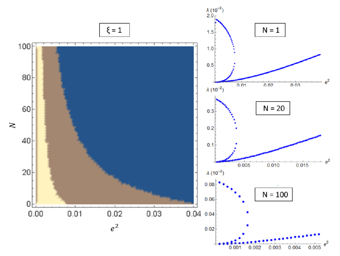
Figure 1: In the left hand side we show a region plot corresponding to the result of scanning for DSB for different values of the free parameters $e^{2}$ and $N$, with $\xi=1$. In our model we find three regions: in the yellow region we have three possible solutions for $\lambda$, in the brown one we have only one solution and in the blue region we do not have solution for $\lambda$, meaning DSB is not operational. In the right hand side, we show a set of plots explicitly showing the behavior of the solutions for $\lambda$ as a function of the $e^{2}$ parameter, for specific values of $N=1,20,100$ and $\xi=1$.

We notice the existence of three regions of solutions for $\lambda$, where the yellow region is characterized by the existence of three different solutions for $\lambda$, which means three different non-symmetric vacua for each value of the parameters within this region. The brown region corresponding to the existence of a single solution, and the blue region with the absence of any solution which breaks symmetry, i.e., for the case when DSB does not happen in our model.

We can analyze the minimum of the effective potential, Eq (59), for example for values of $e^{2}=0.001$, $N=20$ and $\xi=1$, we found the three values of $\lambda$,

$$\lambda_{1}=0.003553,\,\, \lambda_{2}=0.00003590,\,\, \lambda_{3}=0.00001210,$$ (63)

and when these are used together we can see that the minimum occurs as show in figure 2.

Figure 2: This graph of $V_{\mathrm{eff}}\left(\sigma\right)$ vs. $\sigma^{2}/\mu^{2}$ shows the potential minimum for the gauge parameter, $\xi=1$. The effective potential was evaluated using $e^{2}=0.001$, $N=20$ and the values of $\lambda$, as can be seen in Eq. (63). The red rectangle in the botton-left graph is shown in a different scale in the top-right one.

VI Conclusion

In this paper we have studied the behavior of effective potential in a massless Abelian Higgs (AH) model with $N$-component complex scalar field in $(3+1)$ dimensional space-time, specifically concerning its classical vacua structure, obtaining hints of a very rich structure of DSB, depending on the free parameters of the model (the gauge coupling constant and the number of scalar fields). These results were obtained by calculating the effective potential using the RGE equation, and the $\widetilde{\beta}$ and $\widetilde{\gamma}$ functions already reported in the literature. After adapting these renormalization group functions, which were calculated in the minimal subtraction scheme, to a renormalization scheme adequate for our purposes, we shown how the RGE can be used to calculate, order by order in the logarithm $L=\ln\left(\sigma^{2}/\mu^{2}\right)$ and the coupling constants, the effective potential.

Our results points to some interesting prospects, that we intent to approach in future publications. First, to investigate whether further higher-order terms can be incorporated in the effective potential by using a different summation, which could be implemented as a symbolic package for MATHEMATICA, thus further improving our calculation (as it was done in Quinto2016 ). Second, a full study of the Nielsen identity in our model would be important to factor out the possible gauge dependence of the results. Finally, we expect to apply this formalism for other models with application in condensed matter and particle physics in other to study their DBS properties.

Appendix A All coefficients of $B$´s

In this appendix we show the values of the coefficients associated with the functions $B^{\left(3\right)}-B^{\left(5\right)}$ as a function of the Riemann Zeta functions, $\zeta$. In our case we have $\zeta_{3}=\zeta\left(3\right)$ and $\zeta_{5}=\zeta\left(5\right)$ presents in our results. So, we can fix these with $\zeta_{3}=1.202$, known as Apéry’s constant, and $\zeta_{5}=1.036$.

$$b_{1}= \frac{3}{2},\,\,\,b_{2}=\frac{25N}{8}+\frac{27}{2}+\frac{153}{2},\,\,\,b_{3}=\frac{3}{16}\left(47N+119\right),\,\,\,b_{4}=\frac{1}{16}\left(N\left(7N+10\right)-108\right),$$

$$b_{5}= \frac{3}{16}\left(N\left(5N+29\right)+57\right),\,\,\,b_{6}=-\frac{27}{4},\,\,\,b_{7}=\frac{63}{4},$$

$$b_{8}= \frac{1}{192}\left(452N^{2}+648\zeta_{3}\left(3N+5\right)+14433N+33633\right),\,\,\,b_{9}=\frac{21}{8}\left(N+4\right),$$

$$b_{10}= \frac{75\text{$\zeta_{3}$}}{4}+\frac{36599N^{2}}{1728}+\frac{7}{64}\left(673-48\text{$\zeta_{3}$}\right)N-\frac{3029}{32},$$

$$b_{11}= \frac{9}{4}-\frac{7N}{2},\,\,\,b_{12}=\frac{1}{384}\left(-112N^{3}+10541N^{2}-864\zeta_{3}\left(N+19\right)+56043N+139806\right),$$

$$b_{13}= \frac{1}{32}\left(84N^{3}+193N^{2}+72\zeta_{3}\left(N-1\right)-1721N-6432\right),$$

$$b_{14}= \frac{1}{128}\left(456N^{3}+3343N^{2}+144\text{$\zeta_{3}$}\left(5N+11\right)+8739N+11460\right),$$

$$b_{15}= -\frac{9\left(18N+109\right)}{8},\,\,\,b_{16}=\frac{459}{8},\,\,\,b_{17}=\frac{3}{16}\left(N\left(46N+257\right)+493\right),$$

$$b_{18}= \frac{3}{1920}\left(-204000\zeta_{3}+225600\text{$\zeta_{5}$}+608\pi^{4}+5404455\right)$$

$$+\frac{1}{1920}N\left(-35400\zeta_{3}+43200\text{$\zeta_{5}$}+692\pi^{4}+7646330\right)$$

$$+\frac{1}{1920}N^{2}\left(-30\left(1244\zeta_{3}+960\text{$\zeta_{5}$}-67285\right)+5N\left(70N+52113\right)+28\pi^{4}\right),$$

$$b_{19}= +\frac{5}{311040}N^{2}\left(34776N^{2}+1296\zeta_{3}(7N-1444)+11297005N+648\pi^{4}+47536876\right)$$

$$\frac{4787\zeta_{3}}{8}-160\text{$\zeta_{5}$}-\frac{81}{311040}N\left(-222480\zeta_{3}+56\pi^{4}+1962495\right)$$

$$-5\text{$\zeta_{5}$}N\left(N+21\right)+\frac{3\pi^{4}}{40}-\frac{2832569}{384},\,\,\,b_{20}=-\frac{3}{16}\left(5N\left(7N+32\right)+212\right),\,\,\,b_{21}=\frac{9}{2},$$

$$b_{22}= \frac{1}{34560}\left(5N^{2}\left(213840\zeta_{3}-51840\text{$\zeta_{5}$}+17(7987-144\text{$\zeta_{3}$})N-432\pi^{4}+2199556\right)\right)$$

$$-\frac{216N}{34560}\left(-21330\zeta_{3}+18300\text{$\zeta_{5}$}+68\pi^{4}-173865\right)-\frac{135}{34560}\left(64944\zeta_{3}+183840\text{\text{$\zeta_{5}$}}+480\pi^{4}-1275293\right),$$

$$b_{23}= \frac{1}{48}\left(N\left(112N+633\right)+8163\right),$$

$$b_{24}= \frac{1}{17280}\left(4N^{2}\left(90\zeta_{3}(4N+1035)+57175N+162\pi^{4}+2051830\right)\right)$$

$$+\frac{1}{17280}\left(81\left(43920\zeta_{3}+31200\text{$\zeta_{5}$}+132\pi^{4}+520405\right)+9N\left(5\left(78072\zeta_{3}-44640\text{$\zeta_{5}$}+895837\right)+228\pi^{4}\right)\right),$$

$$b_{25}= \frac{9}{8}\left(138-29N\right),$$

$$b_{26}= \frac{1}{3840}N\left(27360\text{$\zeta_{3}$}-72000\text{$\zeta_{5}$}+3N\left(8\left(2760\text{$\zeta_{3}$}+\pi^{4}-73135\right)+5N(4144N+10197)\right)-1008\pi^{4}-10087955\right)$$

$$-\frac{24}{3840}\left(39720\text{$\zeta_{3}$}+9000\text{$\zeta_{5}$}+103\pi^{4}+779815\right),$$

$$b_{27}= \frac{1}{1280}\left(5N^{2}\left(9936\zeta_{3}-1920\text{$\zeta_{5}$}+4848N^{2}+46227N+8\pi^{4}+153516\right)+352\pi^{4}\right)$$

$$+\frac{5}{1280}\left(86064\zeta_{3}-44640\text{$\zeta_{5}$}+226705\right)+\frac{2}{1280}N\left(155040\zeta_{3}-66000\text{$\zeta_{5}$}+124\pi^{4}+576805\right),$$

$$b_{28}= -\frac{333}{4},\,\,\,b_{29}=\frac{1}{96}\left(-N\left(8716N+139815\right)-372249\right),\,\,\,b_{30}=\frac{3}{16}\left(2207N+14742\right),\,\,\,b_{31}=-\frac{9639}{8}.$$ (64)

Appendix B All coefficients for $C$´s

In this appendix we show the values of the coefficients associated with the functions $C^{\left(4\right)}-C^{\left(5\right)}$,

$$c_{1} =\frac{27}{2},\,\,\,c_{2}=\frac{3}{32}\left(N\left(39N+967\right)+3069\right),\,\,\,c_{3}=\frac{1}{32}\left(N\left(298N+1551\right)+522\right),$$

$$c_{4} =\frac{1}{64}\left(N\left(N\left(7N+1255\right)+6897\right)+12042\right),\,\,\,c_{5}=\frac{9}{2}-\frac{21N}{8},$$

$$c_{6} =\frac{3}{16}\left(N\left(N\left(7N+50\right)+94\right)-102\right),\,\,\,c_{7}=\frac{9}{4}\left(N+4\right),\,\,\,c_{8}=\frac{9}{64}\left(N+4\right)\left(N\left(13N+51\right)+95\right),$$

$$c_{9} =-\frac{81}{8}\left(N+12\right),\,\,\,c_{10}=\frac{243}{8},$$

$$c_{11} =\frac{1}{2304}\left(N\left(9072\zeta_{3}+N\left(-32400\zeta_{3}+2\left(99446-21N\right)N+1170811\right)+980397\right)\right)$$

$$+\frac{54}{2304}\left(8832\zeta_{3}-93709\right),\,\,c_{12}=\frac{9}{32}\left(\left(12-7N\right)N+112\right),$$

$$c_{13} =\frac{1}{384}\left(1366N^{3}+648\zeta_{3}\left(6N^{2}+45N+121\right)+89083N^{2}+631260N+1142397\right),$$

$$c_{14} =\frac{1}{128}\left(21N^{4}+11266N^{3}+80917N^{2}-72\zeta_{3}\left(N\left(17N+151\right)+516\right)+256995N+473436\right),$$

$$c_{15} =\frac{9}{16}\left(N\left(13N+82\right)+162\right),$$

$$c_{16} =\frac{3}{256}\left(686N^{4}+3268N^{3}-7937N^{2}+144\zeta_{3}\left(5\left(N-4\right)N-97\right)-74865N-151716\right),$$

$$c_{17} =270-\frac{69N}{16},\,\,\,c_{18}=\frac{9}{2},$$

$$c_{19} =\frac{1}{2304}\left(24743N^{3}+709337N^{2}+2592\zeta_{3}\left(5N\left(2N+15\right)-184\right)+2559492N+5545638\right),$$

$$c_{20} =\frac{1}{16}\left(N\left(35N+219\right)+3330\right),$$

$$c_{21} =\frac{9}{256}\left(270N^{4}+2573N^{3}+8763N^{2}+144\zeta_{3}\left(N+4\right)\left(5N+11\right)+14188N+14238\right),$$

$$c_{22} =-\frac{243}{4},\,\,\,c_{23}=-\frac{3}{32}\left(N\left(457N+9270\right)+35838\right),\,\,\,c_{24}=\frac{81}{16}\left(41N+340\right),\,\,\,c_{25}=-\frac{1215}{2}.$$ (65)

Appendix C All coefficients for $D$´s

In this appendix we show the values of the coefficients associated with the function $D^{\left(5\right)}$,

$$d_{1} =\frac{3}{8}\left(N\left(7N+36\right)+234\right),\,\,\,d_{2}=-\frac{135}{8}\left(N-6\right),\,\,\,d_{3}=\frac{27}{8}\left(N+4\right)^{2},$$

$$d_{4} =\frac{1}{192}\left(N\left(2N\left(616N+15255\right)+118449\right)+142074\right),$$

$$d_{5} =\frac{3}{32}\left(N\left(N\left(33N+1388\right)+11079\right)+23436\right),$$

$$d_{6} =\frac{3}{64}\left(N\left(N\left(7N\left(N+110\right)+5407\right)+12699\right)+14670\right),$$

$$d_{7} =-\frac{9}{16}\left(N+4\right)\left(7N+6\right),\,\,\,d_{8}=\frac{1}{192}\left(N\left(N\left(N\left(7N+5017\right)+38100\right)+106902\right)+58968\right),$$

$$d_{9} =\frac{9}{64}\left(N+4\right)\left(N\left(N\left(21N+142\right)+596\right)+376\right),$$

$$d_{10} =\frac{9}{64}\left(N+4\right)^{2}\left(N\left(23N+49\right)+77\right),\,\,\,d_{11}=-\frac{81}{8}\left(N\left(N+27\right)+129\right),$$

$$d_{12} =\frac{243}{4}\left(N+11\right),\,\,\,d_{13}=-\frac{729}{4}.$$ (66)

References

• [1] J. Zinn-Justin. Quantum field theory and critical phenomena. Clarendon, Oxford, 1996.
• [2] M. E. Peskin. An introduction to quantum field theory. CRCPress, Boca Raton, FL, 2018.
• [3] A. Altland and B. D. Simons. Condensed matter field theory. Cambridge University Press, Cambridge, 2010.
• [4] I. Herbut. A modern approach to critical phenomena. Cambridge University Press, Cambridge, 2007.
• [5] Coleman Sidney and Weinberg Erick. Radiative corrections as the origin of spontaneous symmetry breaking. Phys. Rev. D, 7:1888–1910, Mar 1973.
• [6] V. Elias, R. B. Mann, D. G. C. McKeon, and T. G. Steele. Radiative electroweak symmetry breaking revisited. Phys. Rev. Lett., 91:251601, Dec 2003.
• [7] F. A. Chishtie, V. Elias, R. B. Mann, D. G. C. McKeon, and T. G. Steele. Stability of subsequent-to-leading-logarithm corrections to the effective potential for radiative electroweak symmetry breaking. 743:104–132.
• [8] F. A. Chishtie, T. Hanif, J. Jia, R. B. Mann, D. G. C. McKeon, T. N. Sherry, and T. G. Steele. Can the renormalization group improved effective potential be used to estimate the higgs mass in the conformal limit of the standard model? Phys. Rev. D, 83:105009, May 2011.
• [9] T. G. Steele and Zhi-Wei Wang. Is radiative electroweak symmetry breaking consistent with a 125 gev higgs mass? Phys. Rev. Lett., 110:151601, Apr 2013.
• [10] Boyang Liu, Xiao-Lu Yu, and Wu-Ming Liu. Renormalization-group analysis of $p$-orbital bose-einstein condensates in a square optical lattice. Phys. Rev. A, 88:063605, Dec 2013.
• [11] Shun Uchino. Coleman-weinberg mechanism in spinor bose-einstein condensates. EPL (Europhysics Letters), 107(3):30004, aug 2014.
• [12] I. S. Burmistrov, Y. Gefen, D. S. Shapiro, and A. Shnirman. Mesoscopic stoner instability in open quantum dots: Suppression of coleman-weinberg mechanism by electron tunneling. Phys. Rev. Lett., 124:196801, May 2020.
• [13] Alan Chodos and Hisakazu Minakata. The gross-neveu model as an effective theory for polyacetylene. Phys. Lett. A, 191:39, 1994.
• [14] R. Vega Monroy A. G. Quinto and A. F. Ferrari. Renormalization group improvement of the effective potential in a (1+1) dimensional gross-neveu model. arXiv:2108.04079, 2021.
• [15] M.R. Ahmady, V. Elias, D.G.C. McKeon, A. Squires, and T.G. Steele. Renormalization-group improvement of effective actions beyond summation of leading logarithms. Nuclear Physics B, 655(3):221–249, 2003.
• [16] V. Elias, R. B. Mann, D. G. C. McKeon, and T. G. Steele. Higher order stability of a radiatively induced 220 gev higgs mass. Phys. Rev. D, 72(3):037902, Aug 2005.
• [17] Huan Souza, L. Ibiapina Bevilaqua, and A. C. Lehum. Renormalization group improvement of the effective potential in six dimensions. Phys. Rev. D, 102(4):045004, 2020.
• [18] A.G. Quinto, A.F. Ferrari, and A.C. Lehum. Renormalization group improvement and dynamical breaking of symmetry in a supersymmetric chern-simons-matter model. Nuclear Physics B, 907:664–677, 2016.
• [19] A.G. Dias, J.D. Gomez, A.A. Natale, A.G. Quinto, and A.F. Ferrari. Non-perturbative fixed points and renormalization group improved effective potential. Physics Letters B, 739:8–12, 2014.
• [20] F. A. CHISHTIE, V. ELIAS, R. B. MANN, D. G. C. MCKEON, and T. G. STEELE. On the standard approach to renormalization group improvement. International Journal of Modern Physics E, 16(06):1681–1685, 2007.
• [21] Bernhard Ihrig, Nikolai Zerf, Peter Marquard, Igor F. Herbut, and Michael M. Scherer. Abelian higgs model at four loops, fixed-point collision, and deconfined criticality. Phys. Rev. B, 100:134507, Oct 2019.
• [22] F. A. Chishtie, T. Hanif, D. G. C. McKeon, and T. G. Steele. Unique determination of the effective potential in terms of renormalization group functions. Phys. Rev. D, 77:065007, Mar 2008.
• [23] V. L. Ginzburg and L. D. Landau. On the theory of superconductivity. Zh. Eksp. Teor. Fiz., 20(1064), 1950.
• [24] B. I. Halperin, T. C. Lubensky, and Shang-keng Ma. First-order phase transitions in superconductors and smectic-$a$ liquid crystals. Phys. Rev. Lett., 32:292–295, Feb 1974.
• [25] John C. Collins. Renormalization. Cambridge University Press, 1984.
• [26] Alexander Altland and Ben Simons. Condensed Matter Field Theory. Cambridge, 2010.
• [27] A. G. Dias and A. F. Ferrari. Renormalization group and conformal symmetry breaking in the chern-simons theory coupled to matter. Phys. Rev. D, 82:085006, Oct 2010.
• [28] R. Jackiw. Functional evaluation of the effective potential. Phys. Rev. D, 9:1686–1701, Mar 1974.
• [29] N. K. Nielsen. On the gauge dependence of spontaneous symmetry breaking in gauge theories. Nuclear Physics B, 101(1):173–188, 1975.