Indefinite linear-quadratic optimal control of mean-field stochastic differential equation with jump diffusion: an equivalent cost functional method

Abstract: In this paper, we consider a linear-quadratic optimal control problem of mean-field stochastic differential equation with jump diffusion, which is also called as an MF-LQJ problem. Here, cost functional is allowed to be indefinite. We use an equivalent cost functional method to deal with the MF-LQJ problem with indefinite weighting matrices. Some equivalent cost functionals enable us to establish a bridge between indefinite and positive-definite MF-LQJ problems. With such a bridge, solvabilities of stochastic Hamiltonian system and Riccati equations are further characterized. Optimal control of the indefinite MF-LQJ problem is represented as a state feedback via solutions of Riccati equations. As a by-product, the method provides a new way to prove the existence and uniqueness of solution to mean field forward-backward stochastic differential equation with jump diffusion (MF-FBSDEJ, for short), where existing methods in literature do not work. Some examples are provided to illustrate our results.

Keywords: Equivalent cost functional, Existence and uniqueness of solution to MF-FBSDEJ, Indefinite MF-LQJ problem, Riccati equation, Stochastic Hamiltonian system.

Mathematics Subject Classification: 93E20, 60H10, 34K50

1 Introduction

In recent years, there is an increasing interest in mean-field control theory in mathematics, engineering and finance. Comparing with classical stochastic optimal control, a new feature of this problem is that both objective functional and system dynamics involve states and controls as well as their expected values. There are rich literatures on deriving necessary conditions for optimality. See, for example, Andersson and Djehiche [1], Buckdahn et al. [5], Djehiche et al. [12], Wang et al. [28]. Linear quadratic (LQ, for short) problems of mean-field type have also been investigated. Yong [31] systematically studied an LQ problem of mean-field stochastic differential equation (MF-SDE). Later on, Sun [24] and Li et al. [18] concerned open-loop and closed-loop solvabilities for LQ problems of MF-SDE, respectively. Elliott et al. [13] dealt with an LQ problem of MF-SDE with discrete time setting. Qi et al. [22] investigated stabilization and control problems for linear MF-SDE under standard assumptions. Barreiro-Gomez et al. [2, 3] considered LQ mean-field-type games.

It is well known that jump diffusion processes play an increasing role in describing stochastic dynamical systems, due to its wide application in financial, economic and engineering problems. For example, a geometric Brownian motion is usually used to model stock price, but it cannot reflect discontinuous characteristics, which may be induced by large fluctuations. There are various literatures on related topic. The interested readers may refer to Haadem et al. [14], Øksendal and Sulem [21], Shen et al. [23] for more information. Haadem et al. [14] obtained a maximum principle for jump diffusion process with infinite horizon and dealt an optimal portfolio selection problem. Shen et al. [23] investigated stochastic maximum principle of mean field jump diffusion process with delay and applied their results to a bicriteria mean-variance portfolio selection problem. Øksendal and Sulem [21] systematically discussed optimal control, optimal stopping, and impulse control of jump diffusion processes.

In this paper, a kind of indefinite LQ problem of mean field type jump diffusion process is investigated. Indefinite LQ problems, first studied by Chen et al. [9], have received considerable attention. Chen et al. [10] employed the method of completion of squares to study an indefinite stochastic LQ problem. Huang and Yu [15] and Yu [32] proposed an equivalent cost functional method to deal with stochastic LQ problem with indefinite weighting matrices. Ni et al. [19, 20] considered indefinite LQ problems of discrete-time MF-SDE for an infinite horizon and a finite horizon, respectively. Li et al. [16] studied an indefinite LQ problem of MF-SDE by introducing a relax compensator. Wang et al. [27] concerned with uniform stabilization and social optimality for general mean field LQ control systems, where state weight is not assumed with the definiteness condition. Indefinite MF-LQJ problems, which are natural generalizations of those in [26] and [25], have been not yet completely studied. Tang and Meng [26] investigated a definite MF-LQJ problem in finite horizon and derived two Riccati equations by decoupling optimality system. It was shown that under Assumption (S) given in Section 3 with $S(t)\equiv 0,\bar{S}(t)\equiv 0$, these two Riccati equations are uniquely solvable and a feedback representation for optimal control is obtained. We point out that Assumption (S) is exactly the definite condition when we study an MF-LQJ problem. The MF-LQJ problem reduces to an NC-LQJ problem if $S(t)\equiv 0,\bar{S}(t)\equiv 0$, where “NC” is the capital initials for “no cross”. Tang et al. [25] focused on open-loop and closed-loop solvabilities of an MF-LQJ problem, which extended results in [24, 18]. However, the solvabilities of related Riccati equations without Assumption (S) have not been specified.

Inspired by [15] and [32], we use an equivalent cost functional method to deal with an indefinite MF-LQJ problem. As a preliminary result, we discuss a definite MF-LQJ problem. As mentioned above, the results obtained in [26] are not applicable for solving this MF-LQJ problem. We introduce an invertible linear transformation, which links the MF-LQJ problem with the corresponding NC-LQJ problem. Combining the results in existing literature with this linear transformation, we obtain an optimal control of the MF-LQJ problem under Assumption (S). Then we introduce two auxiliary functions to construct equivalent cost functionals. The original MF-LQJ problem with indefinite control weighting matrices is transformed into an MF-LQJ problem under Assumption (S). In a word, we can investigate the indefinite MF-LQJ problem by using this method.

Our paper distinguishes from existing literature in the following aspects. (i) An indefinite MF-LQJ problem is discussed in this paper, which generalized the results in [26, 25, 16]. The considered model could characterize more general problems and the jump diffusion item is important in some controlled dynamics system. As we will see in Example 5.1, there is no equivalent cost functional satisfying Assumption (S) if jump diffusion item disappears, which implies that we can not construct an optimal control directly in terms of Riccati equations. We further discussed the existence and uniqueness of solutions to the corresponding stochastic Hamiltonian system and Riccati equations without Assumption (S), which have not been considered in [26, 25]. (ii) Compared with derivation of optimal control for the definite NC-LQJ problem in [26], we derive an feedback control of “Problem MF” under Assumption (S) through a simple calculation. Actually, we introduce an invertible linear transformation, which links MF-LQJ problem with the corresponding NC-LQJ problem. (iii) Our results provide an alternative and effective way to obtain the solvability of an MF-FBSDEJ, which does not satisfy classical conditions in existing literature. In fact, when we consider two equivalent cost functionals with the same control system, we can get the equivalence by an invertible linear transformation between the corresponding stochastic Hamiltonian systems. We point out that the equivalence is existed in a family of stochastic Hamiltonian systems. Therefore, we can prove the solvability of a more general MF-FBSDEJ. Moreover, sometimes an MF-FBSDEJ may coincide with the stochastic Hamiltonian system of an MF-LQJ problem, which implies that the solvability of MF-FBSDEJ is actually the solvability of corresponding stochastic Hamiltonian system. Thus, in order to obtain the unique solvability of an MF-FBSDEJ, we need only to find an equivalent cost functional satisfying Assumption (S) of the related MF-LQJ problem. (iv) Relying on the equivalent cost functional method, we can investigate the solvability of indefinite Riccati equations by virtue of the solvability of positive definite Riccati equations. In fact, the original MF-LQJ problem with indefinite control weighting matrices can be transformed into a definite MF-LQJ problem by looking for a simpler and more flexible equivalent cost functional. And there exists an equivalent relation between the corresponding Riccati equations. Similarly, we can get solvabilities of Riccati equations with indefinite condition.

The rest of this paper is organized as follows. In Section 2, we formulate an MF-LQJ problem and give some assumptions throughout this paper. Section 3 aims to study the MF-LQJ problem under Assumption (S). We reduce a general MF-LQJ problem to an NC-LQJ problem via an invertible linear transformation. In Section 4, we present our main results. We use the equivalent cost functional method to study an MF-LQJ problem with indefinite weighting matrices. Section 5 gives several illustrative examples. Finally, in Section 6, we conclude this paper.

2 Problem formulation

Let $\mathbb{R}^{n\times m}$ be an Euclidean space of all $n\times m$ real matrices with inner product $\langle\cdot,\cdot\rangle$ being given by $\langle M,N\rangle\mapsto tr(M^{\top}N)$, where the superscript $\top$ denotes the transpose of vectors or matrices. The induced norm is given by $|M|=\sqrt{tr(M^{\top}M)}$. In particular, we denote by $\mathbb{S}^{n}$ the set of all $n\times n$ symmetric matrices. We mean by an $n\times n$ matrix $N\geq 0$ that $N$ is a nonnegative matrix. Let $T>0$ be a fixed time horizon and $(\Omega,\mathcal{F},\mathbb{F},\mathbb{P})$ be a complete filtered probability space. The filtration $\mathbb{F}\equiv\{\mathcal{F}_{t}\}_{t\geq 0}$ is generated by the following two mutually independent processes, augmented by all the $\mathbb{P}$-null sets: a standard 1-dimensional Brownian motion $W_{t}$ and a Poisson random measure $N(dt,d\theta)$ on $\mathbb{R}_{+}\times\Theta$, where $\Theta\subseteq\mathbb{R}\setminus\{0\}$ is a nonempty set, with compensator $\widehat{N}(dt,d\theta)=\nu(d\theta)dt$, such that $\widetilde{N}([0,t],A)=N([0,t],A)-\widehat{N}([0,t],A)$ is a martingale for all $A\in\mathcal{B}(\Theta)$ satisfying $\nu(A)<\infty$. $\mathcal{B}(\Theta)$ is the Borel $\sigma$-field generated by $\Theta$. Here, $\nu(d\theta)$ is a $\sigma$-finite measure on $(\Theta,\mathcal{B}(\Theta))$ satisfying $\int_{\Theta}(1\wedge\theta^{2})\nu(d\theta)<\infty$, which is called the characteristic measure. Then $\widetilde{N}(dt,d\theta)=N(dt,d\theta)-\nu(d\theta)dt$ is the compensated Poisson random measure. For any Euclidean space $M$, we introduce the following spaces:
$L^{\infty}(0,T;M)=\Big{\{}u:[0,T]\to M|u(\cdot)$ is a bounded function};
$L_{\mathbb{F}}^{2}(0,T;M)=\Big{\{}u:[0,T]\times\Omega\to M|u(\cdot)$ is an $\mathbb{F}$-adapted stochastic process such that $\mathbb{E}\left[\int_{0}^{T}|u(t)|^{2}dt\right]<\infty\Big{\}};$
$S_{\mathbb{F}}^{2}(0,T;M)=\Big{\{}u:[0,T]\times\Omega\to M|u(\cdot)$ is an $\mathbb{F}$-adapted $c\grave{a}dl\grave{a}g$ process in $L_{\mathbb{F}}^{2}(0,T;M)$ such that $\mathbb{E}\big{[}\sup_{t\in[0,T]}|u(t)|^{2}\big{]}<\infty\Big{\}}$;
$L_{\nu}^{2}(M)=\Big{\{}r:[0,T]\times\Theta\to M|r(\cdot)$ is a deterministic function such that $sup_{t\in[0,T]}\int_{\Theta}|r(t,\theta)|^{2}\nu(d\theta)<\infty\Big{\}}$;
$L_{\mathbb{F},\nu}^{2}(0,T;M)=\bigg{\{}r:[0,T]\times\Theta\times\Omega\to M|r(\cdot)$ is an $\mathbb{F}$-predictable stochastic process such that $\mathbb{E}\left[\int_{0}^{T}\int_{\Theta}|r(t,\theta)|^{2}\nu(d\theta)dt\right]<\infty\bigg{\}}$.

Consider a controlled linear MF-SDEJ

$$\left\{\begin{aligned} dX_{t}=&\Big{\{}A_{t}X_{t}+\bar{A}_{t}\mathbb{E}[X_{t}]+B_{t}u_{t}+\bar{B}_{t}\mathbb{E}[u_{t}]\Big{\}}dt\\ &+\Big{\{}C_{t}X_{t}+\bar{C}_{t}\mathbb{E}[X_{t}]+D_{t}u_{t}+\bar{D}_{t}\mathbb{E}[u_{t}]\Big{\}}dW_{t}\\ &+\int_{\Theta}\Big{\{}E_{t,\theta}X_{t-}+\bar{E}_{t,\theta}\mathbb{E}[X_{t-}]+F_{t,\theta}u_{t}+\bar{F}_{t,\theta}\mathbb{E}[u_{t}]\Big{\}}\widetilde{N}(dt,d\theta),\qquad t\in{[0,T]},\\ X_{0}=&\ x\in\mathbb{R}^{n},\end{aligned}\right.$$ (2.1)

where $A_{t},\bar{A}_{t},B_{t},\bar{B}_{t},C_{t},\bar{C}_{t},D_{t},\bar{D}_{t},E_{t,\theta},\bar{E}_{t,\theta},F_{t,\theta},\bar{F}_{t,\theta}$ are given matrix valued deterministic functions. In the above equation, $u$, valued in $\mathbb{R}^{m}$, is a control process and $X$, valued in $\mathbb{R}^{n}$, is the corresponding state process. In this paper, an admissible control $u$ is defined as a predictable process such that $u\in L_{\mathbb{F}}^{2}(0,T;\mathbb{R}^{m})$. The set of all admissible controls is denoted by $\mathcal{U}[0,T]$. We introduce a cost functional

$$J[u]= \ \frac{1}{2}\mathbb{E}\left\{\langle GX_{T},X_{T}\rangle+\langle\bar{G}\mathbb{E}[X_{T}],\mathbb{E}[X_{T}]\rangle\right.$$ (2.2)

$$+\int_{0}^{T}\left\langle\left(\begin{array}[]{cc}Q_{t}&S_{t}\\ S_{t}^{\top}&R_{t}\end{array}\right)\left(\begin{array}[]{c}X_{t}\\ u_{t}\end{array}\right),\left(\begin{array}[]{c}X_{t}\\ u_{t}\end{array}\right)\right\rangle dt$$

$$+\left.\int_{0}^{T}\left\langle\left(\begin{array}[]{cc}\bar{Q}_{t}&\bar{S}_{t}\\ \bar{S}_{t}^{\top}&\bar{R}_{t}\end{array}\right)\left(\begin{array}[]{c}\mathbb{E}[X_{t}]\\ \mathbb{E}[u_{t}]\end{array}\right),\left(\begin{array}[]{c}\mathbb{E}[X_{t}]\\ \mathbb{E}[u_{t}]\end{array}\right)\right\rangle dt\right\},$$

where $G,\bar{G}$ are symmetric matrices and $Q_{t},S_{t},R_{t},\bar{Q}_{t},\bar{S}_{t},\bar{R}_{t}$ are deterministic matrix-valued functions with $Q_{t}=Q_{t}^{\top},R_{t}=R_{t}^{\top},\bar{Q}_{t}=\bar{Q}_{t}^{\top},\bar{R}_{t}=\bar{R}_{t}^{\top}$. Our MF-LQJ problem is stated as follows.
Problem MF: For any $x\in\mathbb{R}^{n}$, find a $u^{*}\in\mathcal{U}[0,T]$ such that

$$J[u^{*}]=\inf_{u\in\mathcal{U}[0,T]}J[u].$$ (2.3)

Any $u^{*}\in\mathcal{U}[0,T]$ satisfying (2.3) is called an optimal control of Problem MF, and the corresponding state process $X^{*}=X(x,u^{*})$ is called an optimal state process. $(X^{*},u^{*})$ is called an optimal pair.

The following assumptions will be in force throughout this paper.
(H1) The coefficients of state equation satisfy

$$\left\{\begin{array}[]{l}A,\bar{A},C,\bar{C}\in L^{\infty}(0,T;\mathbb{R}^{n\times n}),B,\bar{B},D,\bar{D}\in L^{\infty}(0,T;\mathbb{R}^{n\times m}),\\ E,\bar{E}\in L_{\nu}^{2}(\mathbb{R}^{n\times n}),F,\bar{F}\in L_{\nu}^{2}(\mathbb{R}^{n\times m}).\end{array}\right.$$

(H2) The weighting matrices in cost functional satisfy

$$\left\{\begin{aligned} &Q,\bar{Q}\in L^{\infty}(0,T;\mathbb{S}^{n}),\ R,\bar{R}\in L^{\infty}(0,T;\mathbb{S}^{m}),\\ &S,\bar{S}\in L^{\infty}(0,T;\mathbb{R}^{n\times m}),\ G,\bar{G}\in\mathbb{S}^{n}.\end{aligned}\right.$$

We can show that under (H1), for any $u\in\mathcal{U}[0,T]$, (2.1) admits a unique solution $X=X(x,u)\in S_{\mathbb{F}}^{2}(0,T;\mathbb{R}^{n})$.

3 MF-LQJ problem under standard conditions

In this section, we aim at studying Problem MF under some standard conditions. We introduce an invertible linear transformation, which links MF-LQJ problem with the corresponding NC-LQJ problem.
Assumption (S): For some $\alpha_{0}>0$,

$$\left\{\begin{aligned} &R_{t},R_{t}+\bar{R}_{t}\geq\alpha_{0}I,Q_{t}-S_{t}R_{t}^{-1}S_{t}^{\top}\geq 0,\\ &Q_{t}+\bar{Q}_{t}-(S_{t}+\bar{S}_{t})(R_{t}+\bar{R}_{t})^{-1}(S_{t}+\bar{S}_{t})^{\top}\geq 0,\quad t\in[0,T],\\ &G,G+\bar{G}\geq 0.\end{aligned}\right.$$

We introduce a stochastic Hamiltonian system related to Problem MF

$$\left\{\begin{aligned} &dX_{t}=\Big{\{}A_{t}X_{t}+\bar{A}_{t}\mathbb{E}[X_{t}]+B_{t}u_{t}+\bar{B}_{t}\mathbb{E}[u_{t}]\Big{\}}dt\\ &\qquad\ \ \ +\Big{\{}C_{t}X_{t}+\bar{C}_{t}\mathbb{E}[X_{t}]+D_{t}u_{t}+\bar{D}_{t}\mathbb{E}[u_{t}]\Big{\}}dW_{t}\\ &\qquad\ \ \ +\int_{\Theta}\Big{\{}E_{t,\theta}X_{t-}+\bar{E}_{t,\theta}\mathbb{E}[X_{t-}]+F_{t,\theta}u_{t}+\bar{F}_{t,\theta}\mathbb{E}[u_{t}]\Big{\}}\widetilde{N}(dt,d\theta),\\ &dY_{t}=-\Big{\{}A_{t}^{\top}Y_{t}+\bar{A}_{t}^{\top}\mathbb{E}[Y_{t}]+C_{t}^{\top}Z_{t}+\bar{C}_{t}^{\top}\mathbb{E}[Z_{t}]+\int_{\Theta}\Big{(}E_{t,\theta}^{\top}r_{t,\theta}+\bar{E}_{t,\theta}^{\top}\mathbb{E}[r_{t,\theta}]\Big{)}\nu(d\theta)\\ &\qquad\ \ \ +Q_{t}X_{t}+\bar{Q}_{t}\mathbb{E}[X_{t}]+S_{t}u_{t}+\bar{S}_{t}\mathbb{E}[u_{t}]\Big{\}}dt+Z_{t}dW_{t}+\int_{\Theta}r_{t,\theta}\widetilde{N}(dt,d\theta),\\ &X_{0}=x,\ \ \ \ Y_{T}=GX_{T}+\bar{G}\mathbb{E}[X_{T}],\\ &R_{t}u_{t}+\bar{R}_{t}\mathbb{E}[u_{t}]+S_{t}^{\top}X_{t-}+\bar{S}_{t}^{\top}\mathbb{E}[X_{t-}]+B_{t}^{\top}Y_{t-}+\bar{B}_{t}^{\top}\mathbb{E}[Y_{t-}]\\ &\ \ +D_{t}^{\top}Z_{t}+\bar{D}_{t}^{\top}\mathbb{E}[Z_{t}]+\int_{\Theta}\left(F_{t,\theta}^{\top}r_{t,\theta}+\bar{F}_{t,\theta}^{\top}\mathbb{E}[r_{t,\theta}]\right)\nu(d\theta)=0.\end{aligned}\right.$$ (3.1)

Using the method in [26], we decouple the above Hamiltonian system and derive Riccati equations associated with Problem MF

$$\left\{\begin{aligned} &\dot{P_{t}}+P_{t}A_{t}+A_{t}^{\top}P_{t}+C_{t}^{\top}P_{t}C_{t}+\int_{\Theta}E_{t,\theta}^{\top}P_{t}E_{t,\theta}\nu(d\theta)+Q_{t}\\ &\ -\left(S_{t}+P_{t}B_{t}+C_{t}^{\top}P_{t}D_{t}+\int_{\Theta}E_{t,\theta}^{\top}P_{t}F_{t,\theta}\nu(d\theta)\right)\Sigma_{0t}^{-1}\\ &\ \cdot\left(S_{t}^{\top}+B_{t}^{\top}P_{t}+D_{t}^{\top}P_{t}C_{t}+\int_{\Theta}F_{t,\theta}^{\top}P_{t}E_{t,\theta}\nu(d\theta)\right)=0,\\ &P_{T}=G,\end{aligned}\right.$$ (3.2)

$$\left\{\begin{aligned} &\dot{\Pi_{t}}+\Pi_{t}(A_{t}+\bar{A}_{t})+(A_{t}+\bar{A}_{t})^{\top}\Pi_{t}+(C_{t}+\bar{C}_{t})^{\top}P_{t}(C_{t}+\bar{C}_{t})\\ &\ +\int_{\Theta}(E_{t,\theta}+\bar{E}_{t,\theta})^{\top}P_{t}(E_{t,\theta}+\bar{E}_{t,\theta})\nu(d\theta)+Q_{t}+\bar{Q}_{t}\\ &\ -\left[(S_{t}+\bar{S}_{t})+\Pi_{t}(B_{t}+\bar{B}_{t})+(C_{t}+\bar{C}_{t})^{\top}P_{t}(D_{t}+\bar{D}_{t})\right.\\ &\ \left.+\int_{\Theta}(E_{t,\theta}+\bar{E}_{t,\theta})^{\top}P_{t}(F_{t,\theta}+\bar{F}_{t,\theta})\nu(d\theta)\right]\Sigma_{1t}^{-1}\\ &\ \cdot\left[(S_{t}+\bar{S}_{t})^{\top}+(B_{t}+\bar{B}_{t})^{\top}\Pi_{t}+(D_{t}+\bar{D}_{t})^{\top}P_{t}(C_{t}+\bar{C}_{t})\right.\\ &\ +\left.\int_{\Theta}(F_{t,\theta}+F_{t,\theta})^{\top}P_{t}(E_{t,\theta}+E_{t,\theta})\nu(d\theta)\right]=0,\\ &\Pi_{T}=G+\bar{G},\end{aligned}\right.$$ (3.3)

where

$$\Sigma_{0t}=R_{t}+D_{t}^{\top}P_{t}D_{t}+\int_{\Theta}F_{t,\theta}^{\top}P_{t}F_{t,\theta}\nu(d\theta),$$

$$\Sigma_{1t}=R_{t}+\bar{R}_{t}+(D_{t}+\bar{D}_{t})^{\top}P_{t}(D_{t}+\bar{D}_{t})+\int_{\Theta}(F_{t,\theta}+F_{t,\theta})^{\top}P_{t}(F_{t,\theta}+F_{t,\theta})\nu(d\theta).$$

Note that (3.1) is a coupled MF-FBSDEJ, where the coupling comes from the last relation (which is essentially the maximum condition in the usual Pontryagin type maximum principle). Different from an NC-LQJ problem, there are additional items $2\langle X_{t},S_{t}u_{t}\rangle$ and $2\langle\mathbb{E}[X_{t}],\bar{S}_{t}\mathbb{E}[u_{t}]\rangle$ in cost functional (2.2). Next, we want to reduce Problem MF to an NC-LQJ problem. For this, we introduce a controlled system

$$\left\{\begin{aligned} d\tilde{X}_{t}=&\ \Big{\{}A_{1t}(\tilde{X}_{t}-\mathbb{E}[\tilde{X}_{t}])+B_{t}\tilde{u}_{t}+[A_{1t}+\bar{A}_{1t}]\mathbb{E}[\tilde{X}_{t}]+\bar{B}_{t}\mathbb{E}[\tilde{u}_{t}]\Big{\}}dt\\ &+\Big{\{}C_{1t}(\tilde{X}_{t}-\mathbb{E}[\tilde{X}_{t}])+D_{t}\tilde{u}_{t}+[C_{1t}+\bar{C}_{1t}]\mathbb{E}[\tilde{X}_{t}]+\bar{D}_{t}\mathbb{E}[\tilde{u}_{t}]\Big{\}}dW_{t}\\ &+\int_{\Theta}\Big{\{}E_{1t,\theta}(\tilde{X}_{t-}-\mathbb{E}[\tilde{X}_{t-}])+F_{t,\theta}\tilde{u}_{t}+[E_{1t,\theta}+\bar{E}_{1t,\theta}]\mathbb{E}[\tilde{X}_{t-}]+\bar{F}_{t,\theta}\mathbb{E}[\tilde{u}_{t}]\Big{\}}\widetilde{N}(dt,d\theta),\\ \tilde{X}_{0}=\ &x,\end{aligned}\right.$$ (3.4)

and a cost functional

$$\tilde{J}[\tilde{u}]=\frac{1}{2}\mathbb{E}\left\{\langle G\tilde{X}_{T},\tilde{X}_{T}\rangle+\langle\bar{G}\mathbb{E}[\tilde{X}_{T}],\mathbb{E}[\tilde{X}_{T}]\rangle\right.$$ (3.5)

$$\ \ +\int_{0}^{T}\left\langle\left(\begin{array}[]{cc}Q_{1t}&\mathbf{0}_{n\times m}\\ \mathbf{0}_{m\times n}&R_{t}\end{array}\right)\left(\begin{array}[]{c}\tilde{X}_{t}-\mathbb{E}[\tilde{X}_{t}]\\ \tilde{u}_{t}-\mathbb{E}[\tilde{u}_{t}]\end{array}\right),\left(\begin{array}[]{c}\tilde{X}_{t}-\mathbb{E}[\tilde{X}_{t}]\\ \tilde{u}_{t}-\mathbb{E}[\tilde{u}_{t}]\end{array}\right)\right\rangle dt$$

$$\ \ \left.+\int_{0}^{T}\left\langle\left(\begin{array}[]{cc}Q_{1t}+\bar{Q}_{1t}&\mathbf{0}_{n\times m}\\ \mathbf{0}_{m\times n}&R_{t}+\bar{R}_{t}\end{array}\right)\left(\begin{array}[]{c}\mathbb{E}[\tilde{X}_{t}]\\ \mathbb{E}[\tilde{u}_{t}]\end{array}\right),\left(\begin{array}[]{c}\mathbb{E}[\tilde{X}_{t}]\\ \mathbb{E}[\tilde{u}_{t}]\end{array}\right)\right\rangle dt\right\},$$

where

$$A_{1t}=A_{t}-B_{t}R_{t}^{-1}S_{t}^{\top},$$

$$A_{1t}+\bar{A}_{1t}=A_{t}+\bar{A}_{t}-(B_{t}+\bar{B}_{t})(R_{t}+\bar{R}_{t})^{-1}(S_{t}+\bar{S}_{t})^{\top},$$

$$C_{1t}=C_{t}-D_{t}R_{t}^{-1}S_{t}^{\top},$$

$$C_{1t}+\bar{C}_{1t}=C_{t}+\bar{C}_{t}-(D_{t}+\bar{D}_{t})(R_{t}+\bar{R}_{t})^{-1}(S_{t}+\bar{S}_{t})^{\top},$$

$$E_{1t,\theta}=E_{t,\theta}-F_{t,\theta}R_{t}^{-1}S_{t}^{\top},$$

$$E_{1t,\theta}+\bar{E}_{1t,\theta}=E_{t,\theta}+\bar{E}_{t,\theta}-(F_{t,\theta}+\bar{F}_{t,\theta})(R_{t}+\bar{R}_{t})^{-1}(S_{t}+\bar{S}_{t})^{\top},$$

$$Q_{1t}=Q_{t}-S_{t}R_{t}^{-1}S_{t}^{\top},$$

$$Q_{1t}+\bar{Q}_{1t}=Q_{t}+\bar{Q}_{t}-(S_{t}+\bar{S}_{t})(R_{t}+\bar{R}_{t})^{-1}(S_{t}+\bar{S}_{t})^{\top}.$$

The corresponding NC-LQJ problem is stated as follows.

Problem NC: For any $x\in\mathbb{R}^{n}$, find a $\tilde{u}^{*}\in\mathcal{U}[0,T]$ such that

$$\tilde{J}[\tilde{u}^{*}]=\inf_{\tilde{u}\in\mathcal{U}[0,T]}\tilde{J}[\tilde{u}].$$ (3.6)

Similar to Problem MF, we write the stochastic Hamiltonian system and Riccati equations corresponding to Problem NC

$$\left\{\begin{aligned} &d\tilde{X}_{t}=\left\{A_{1t}\tilde{X}_{t}+\bar{A}_{1t}\mathbb{E}[\tilde{X}_{t}]+B_{t}\tilde{u}_{t}+\bar{B}_{t}\mathbb{E}[\tilde{u}_{t}]\right\}dt\\ &\ \ \ \ \ \ \ +\left\{C_{1t}\tilde{X}_{t}+\bar{C}_{1t}\mathbb{E}[\tilde{X}_{t}]+D_{t}\tilde{u}_{t}+\bar{D}_{t}\mathbb{E}[\tilde{u}_{t}]\right\}dW_{t}\\ &\ \ \ \ \ \ \ +\int_{\Theta}\Big{\{}E_{1t,\theta}\tilde{X}_{t-}+\bar{E}_{1t,\theta}\mathbb{E}[\tilde{X}_{t-}]+F_{t,\theta}\tilde{u}_{t}+\bar{F}_{t,\theta}\mathbb{E}[\tilde{u}_{t}]\Big{\}}\widetilde{N}(dt,d\theta),\\ &d\tilde{Y}_{t}=-\Big{\{}A_{1t}^{\top}\tilde{Y}_{t}+\bar{A}_{1t}^{\top}\mathbb{E}[\tilde{Y}_{t}]+C_{1t}^{\top}\tilde{Z}_{t}+\bar{C}_{1t}^{\top}\mathbb{E}[\tilde{Z}_{t}]+\int_{\Theta}\Big{(}E_{1t,\theta}^{\top}\tilde{r}_{t,\theta}+\bar{E}_{1t,\theta}^{\top}\mathbb{E}[\tilde{r}_{t,\theta}]\Big{)}\nu(d\theta)\\ &\ \ \ \ \ \ \ +Q_{1t}\tilde{X}_{t}+\bar{Q}_{1t}\mathbb{E}[\tilde{X}_{t}]\Big{\}}dt+\tilde{Z}_{t}dW_{t}+\int_{\Theta}\tilde{r}_{t,\theta}\widetilde{N}(dt,d\theta),\\ &\tilde{X}_{0}=x,\ \ \ \ \tilde{Y}_{T}=G\tilde{X}_{T}+\bar{G}\mathbb{E}[\tilde{X}_{T}],\\ &R_{t}\tilde{u}_{t}+\bar{R}_{t}\mathbb{E}[\tilde{u}_{t}]+B_{t}^{\top}\tilde{Y}_{t-}+\bar{B}_{t}^{\top}\mathbb{E}[\tilde{Y}_{t-}]+D_{t}^{\top}\tilde{Z}_{t}+\bar{D}_{t}^{\top}\mathbb{E}[\tilde{Z}_{t}]\\ &+\int_{\Theta}\left(F_{t,\theta}^{\top}\tilde{r_{t,\theta}}+\bar{F}_{t,\theta}^{\top}\mathbb{E}[\tilde{r_{t,\theta}}]\right)\nu(d\theta)=0,\end{aligned}\right.$$ (3.7)

$$\left\{\begin{aligned} &\dot{P_{t}}+P_{t}A_{1t}+A_{1t}^{\top}P_{t}+C_{1t}^{\top}P_{t}C_{1t}+\int_{\Theta}E_{1t,\theta}^{\top}P_{t}E_{1t,\theta}\nu(d\theta)+Q_{1t}\\ &\quad-\left(P_{t}B_{t}+C_{1t}^{\top}P_{t}D_{t}+\int_{\Theta}E_{1t,\theta}^{\top}P_{t}F_{t,\theta}\nu(d\theta)\right)\Sigma_{0t}^{-1}\\ &\quad\cdot\left(B_{t}^{\top}P_{t}+D_{t}^{\top}P_{t}C_{1t}+\int_{\Theta}F_{t,\theta}^{\top}P_{t}E_{1t,\theta}\nu(d\theta)\right)=0,\\ &P_{T}=G,\end{aligned}\right.$$ (3.8)

$$\left\{\begin{aligned} &\dot{\Pi_{t}}+\Pi_{t}\left(A_{1t}+\bar{A}_{1t}\right)+\left(A_{1t}+\bar{A}_{1t}\right)^{\top}\Pi_{t}+\left(C_{1t}+\bar{C}_{1t}\right)^{\top}P_{t}\left(C_{1t}+\bar{C}_{1t}\right)\\ &\quad+\int_{\Theta}(E_{1t,\theta}+\bar{E}_{1t,\theta})^{\top}P_{t}(E_{1t,\theta}+\bar{E}_{1t,\theta})\nu(d\theta)+Q_{1t}+\bar{Q}_{1t}\\ &\quad-\left[\Pi_{t}(B_{t}+\bar{B}_{t})+(C_{1t}+\bar{C}_{1t})^{\top}P_{t}(D_{t}+\bar{D}_{t})+\int_{\Theta}(E_{1t,\theta}+\bar{E}_{1t,\theta})^{\top}P_{t}(F_{t,\theta}+\bar{F}_{t,\theta})\nu(d\theta)\right]\Sigma_{1t}^{-1}\\ &\quad\cdot\left[(B_{t}+\bar{B}_{t})^{\top}\Pi_{t}+(D_{t}+\bar{D}_{t})^{\top}P_{t}(C_{1t}+\bar{C}_{1t})+\int_{\Theta}(F_{t,\theta}+F_{t,\theta})^{\top}P_{t}(E_{1t,\theta}+E_{1t,\theta})\nu(d\theta)\right]=0,\\ &\Pi_{T}=G+\bar{G},\end{aligned}\right.$$ (3.9)

where

$$\Sigma_{0t}=R_{t}+D_{t}^{\top}P_{t}D_{t}+\int_{\Theta}F_{t,\theta}^{\top}P_{t}F_{t,\theta}\nu(d\theta),$$

$$\Sigma_{1t}=R_{t}+\bar{R}_{t}+(D_{t}+\bar{D}_{t})^{\top}P_{t}(D_{t}+\bar{D}_{t})+\int_{\Theta}(F_{t,\theta}+F_{t,\theta})^{\top}P_{t}(F_{t,\theta}+F_{t,\theta})\nu(d\theta).$$

Lemma 3.1.

Let Assumption (S) hold. For any two pairs $(X,u)$ and $(\tilde{X},\tilde{u})$, we introduce a linear transformation

$$\left(\begin{array}[]{c}X-\mathbb{E}[X]\\ u-\mathbb{E}[u]\end{array}\right)=\left(\begin{array}[]{cc}I_{n\times n}&\mathbf{0}_{n\times m}\\ -R^{-1}S^{\top}&I_{m\times m}\end{array}\right)\left(\begin{array}[]{c}\tilde{X}-\mathbb{E}[\tilde{X}]\\ \tilde{u}-\mathbb{E}[\tilde{u}]\end{array}\right),$$ (3.10)

$$\left(\begin{array}[]{c}\mathbb{E}[X]\\ \mathbb{E}[u]\end{array}\right)=\left(\begin{array}[]{cc}I_{n\times n}&\mathbf{0}_{n\times m}\\ -(R+\bar{R})^{-1}(S+\bar{S})^{\top}&I_{m\times m}\end{array}\right)\left(\begin{array}[]{c}\mathbb{E}[\tilde{X}]\\ \mathbb{E}[\tilde{u}]\end{array}\right).$$ (3.11)

Then the following two statements are equivalent:

• $(X,u)$ is an admissible (optimal) control of Problem MF.

• $(\tilde{X},\tilde{u})$ is an admissible (optimal) control of Problem NC.

Moreover, we have $J[u]=\tilde{J}[\tilde{u}].$

Proof.

It follows from (3.10) and (3.11) that

$$\left(\begin{array}[]{c}\tilde{X}-\mathbb{E}[\tilde{X}]\\ \tilde{u}-\mathbb{E}[\tilde{u}]\end{array}\right)=\left(\begin{array}[]{cc}I_{n\times n}&\mathbf{0}_{n\times m}\\ R^{-1}S^{\top}&I_{m\times m}\end{array}\right)\left(\begin{array}[]{c}X-\mathbb{E}[X]\\ u-\mathbb{E}[u]\end{array}\right),$$

$$\left(\begin{array}[]{c}\mathbb{E}[\tilde{X}]\\ \mathbb{E}[\tilde{u}]\end{array}\right)=\left(\begin{array}[]{cc}I_{n\times n}&\mathbf{0}_{n\times m}\\ (R+\bar{R})^{-1}(S+\bar{S})^{\top}&I_{m\times m}\end{array}\right)\left(\begin{array}[]{c}\mathbb{E}[X]\\ \mathbb{E}[u]\end{array}\right).$$

Then linear transformation (3.10) with (3.11) is invertible. Through direct calculation, it is easy to verify statement (i) is equivalent to statement (ii) , and thus $J[u]=\tilde{J}[\tilde{u}].$ ∎

The above lemma tells us that there exists some equivalent relationship between Problem MF and Problem NC. We now analyze the relationship in terms of stochastic Hamiltonian system and Riccati equations, respectively.

Lemma 3.2.

Under Assumption (S), $(\tilde{X}^{*},\tilde{u}^{*},Y,Z,r)$ is the solution of (3.7) if and only if $(X^{*},u^{*},Y,Z,r)$ is the solution of (3.1).

Proof.

According to Lemma 3.1, it is not difficult to draw the conclusion.

∎

Lemma 3.3.

Under Assumption (S), we have

• Riccati equations (3.8) and (3.2) are the same.

• Riccati equations (3.9) and (3.3) are the same.

Proof.

For simplicity of notations, we denote

$$G(A_{t},B_{t},C_{t},D_{t},E_{t,\theta},F_{t,\theta};Q_{t},R_{t},S_{t};P_{t})$$

$$= \ P_{t}A_{t}+A_{t}^{\top}P_{t}+C_{t}^{\top}P_{t}C_{t}+\int_{\Theta}E_{t,\theta}^{\top}P_{t}E_{t,\theta}\nu(d\theta)+Q_{t}$$

$$-\left(P_{t}B_{t}+C_{t}^{\top}P_{t}D_{t}+\int_{\Theta}E_{t,\theta}^{\top}P_{t}F_{t,\theta}\nu(d\theta)+S_{t}\right)\Sigma_{0t}^{-1}$$

$$\cdot\left(B_{t}^{\top}P_{t}+D_{t}^{\top}P_{t}C_{t}+\int_{\Theta}F_{t,\theta}^{\top}P_{t}E_{t,\theta}\nu(d\theta)+S_{t}^{\top}\right).$$

It is enough to prove $G(A_{t},B_{t},C_{t},D_{t},E_{t,\theta},F_{t,\theta};Q_{t},R_{t},S_{t};P_{t})=G(A_{1t},B_{t},C_{1t},D_{t},E_{1t,\theta},F_{t,\theta};Q_{1t},R_{t},\mathbf{0};P_{t})$. We have

$$\Sigma_{0t}^{-1}\left(B_{t}^{\top}P_{t}+D_{t}^{\top}P_{t}C_{t}+\int_{\Theta}F_{t,\theta}^{\top}P_{t}E_{t,\theta}\nu(d\theta)+S_{t}^{\top}\right)$$

$$-\Sigma_{0t}^{-1}\left(B_{t}^{\top}P_{t}+D_{t}^{\top}P_{t}C_{1t}+\int_{\Theta}F_{t,\theta}^{\top}P_{t}E_{1t,\theta}\nu(d\theta)\right)$$

$$= \ \Sigma_{0t}^{-1}\left(D_{t}^{\top}P_{t}D_{t}+\int_{\Theta}F_{t,\theta}^{\top}P_{t}F_{t,\theta}\nu(d\theta)+R_{t}\right)R_{t}^{-1}S_{t}^{\top}$$

$$= \ R_{t}^{-1}S_{t}^{\top}.$$

Thus, we calculate

$$G(A_{t},B_{t},C_{t},D_{t},E_{t,\theta},F_{t,\theta};Q_{t},R_{t},S_{t};P_{t})-G(A_{1t},B_{t},C_{1t},D_{t},E_{1t,\theta},F_{t,\theta};Q_{1t},R_{t},\mathbf{0};P_{t})$$

$$= \ P_{t}B_{t}R_{t}^{-1}S_{t}^{\top}+S_{t}R_{t}^{-1}B_{t}^{\top}P_{t}+C_{t}^{\top}P_{t}D_{t}R_{t}^{-1}S_{t}^{\top}+S_{t}R_{t}^{-1}D_{t}^{\top}P_{t}C_{1t}$$

$$+\int_{\Theta}E_{t,\theta}^{\top}P_{t}F_{t,\theta}R_{t}^{-1}S_{t}^{\top}\nu(d\theta)+\int_{\Theta}S_{t}R_{t}^{-1}F_{t,\theta}^{\top}P_{t,\theta}E_{1t,\theta}\nu(d\theta)$$

$$+S_{t}R_{t}^{-1}S_{t}^{\top}-\left(S_{t}+P_{t}B_{t}+C_{t}^{\top}P_{t}D_{t}+\int_{\Theta}E_{t,\theta}^{\top}P_{t}F_{t,\theta}\nu(d\theta)\right)R_{t}^{-1}S_{t}^{\top}$$

$$-S_{t}R_{t}^{-1}\left(B_{t}^{\top}P_{t}+D_{t}^{\top}P_{t}C_{1t}+\int_{\Theta}F_{t,\theta}^{\top}P_{t}E_{1t,\theta}\nu(d\theta)\right)$$

$$= \ \mathbf{0}_{n\times n}.$$

Consequently, we complete the proof. ∎

We cite a result in [26], which plays a role in deriving an optimal control of Problem MF under standard condition.

Lemma 3.4.

Let (H1)-(H2) and Assumption (S) hold, then Riccati equations (3.8) and (3.9) admit unique solutions $P$ and $\Pi$, respectively. Further, the optimal pair $(\tilde{X}^{*},\tilde{u}^{*})$ of Problem NC satisfies

$$\left\{\begin{aligned} \tilde{u}_{t}^{*}=&-\Sigma_{0t}^{-1}\left(B_{t}^{\top}P_{t}+D_{t}^{\top}P_{t}C_{1t}+\int_{\Theta}F_{t,\theta}^{\top}P_{t}E_{1t,\theta}\nu(d\theta)\right)(\tilde{X}_{t}^{*}-\mathbb{E}[\tilde{X}_{t}^{*}])\\ &-\Sigma_{1t}^{-1}\left[(B_{t}+\bar{B}_{t})^{\top}\Pi_{t}+(D_{t}+\bar{D}_{t})^{\top}P_{t}(C_{1t}+\bar{C}_{1t})\right.\\ &+\left.\int_{\Theta}(F_{t,\theta}+\bar{F}_{t,\theta})^{\top}P_{t}(E_{1t,\theta}+\bar{E}_{1t,\theta})\nu(d\theta)\right]\mathbb{E}[\tilde{X}_{t}^{*}],\\ d\tilde{X}_{t}^{*}=&\ \Big{\{}A_{1t}\tilde{X}_{t}^{*}+\bar{A}_{1t}\mathbb{E}[\tilde{X}_{t}^{*}]+B_{t}\tilde{u}_{t}^{*}+\bar{B}_{t}\mathbb{E}[\tilde{u}_{t}^{*}]\Big{\}}dt\\ &+\Big{\{}C_{1t}\tilde{X}_{t}^{*}+\bar{C}_{1t}\mathbb{E}[\tilde{X}_{t}^{*}]+D_{t}\tilde{u}_{t}^{*}+\bar{D}_{t}\mathbb{E}[\tilde{u}_{t}^{*}]\Big{\}}dW_{t}\\ &+\int_{\Theta}\Big{\{}E_{1t,\theta}\tilde{X}_{t-}^{*}+\bar{E}_{1t,\theta}\mathbb{E}[\tilde{X}_{t-}^{*}]+F_{t,\theta}\tilde{u}_{t}^{*}+\bar{F}_{t,\theta}\mathbb{E}[\tilde{u}_{t}^{*}]\Big{\}}\widetilde{N}(dt,d\theta),\\ \tilde{X}_{0}^{*}=&\ x.\end{aligned}\right.$$

Defining

$$\left\{\begin{aligned} \tilde{Y}_{t}^{*}=&\ P_{t}(\tilde{X}_{t}^{*}-\mathbb{E}[\tilde{X}_{t}^{*}])+\Pi_{t}\mathbb{E}[\tilde{X}_{t}^{*}],\\ \tilde{Z}_{t}^{*}=&\ \left[P_{t}C_{1t}-P_{t}D_{t}\Sigma_{0t}^{-1}\left(B_{t}^{\top}P_{t}+D_{t}^{\top}P_{t}C_{1t}+\int_{\Theta}F_{t,\theta}^{\top}P_{t}E_{1t,\theta}\nu(d\theta)\right)\right](\tilde{X}_{t}^{*}-\mathbb{E}[\tilde{X}_{t}^{*}])\\ &+\left\{P_{t}(C_{1t}+\bar{C}_{1t})-P_{t}(D_{t}+\bar{D}_{t})\Sigma_{1t}^{-1}\left[(B_{t}+\bar{B}_{t})^{\top}\Pi_{t}+(D_{t}+\bar{D}_{t})^{\top}P_{t}(C_{1t}+\bar{C}_{1t})\right.\right.\\ &\left.\left.+\int_{\Theta}(F_{t,\theta}+\bar{F}_{t,\theta})^{\top}P_{t}(E_{1t,\theta}+\bar{E}_{1t,\theta})\nu(d\theta)\right]\right\}\mathbb{E}[\tilde{X}_{t}^{*}],\\ \tilde{r}_{t,\theta}^{*}=&\ \left[P_{t}E_{1t,\theta}-P_{t}F_{t,\theta}\Sigma_{0t}^{-1}\left(B_{t}^{\top}P_{t}+D_{t}^{\top}P_{t}C_{1t}+\int_{\Theta}F_{t,\theta}^{\top}P_{t}E_{1t,\theta}\nu(d\theta)\right)\right](\tilde{X}_{t}^{*}-\mathbb{E}[\tilde{X}_{t}^{*}])\\ &+\Big{\{}P_{t}(E_{1t,\theta}+\bar{E}_{1t,\theta})-P_{t}(F_{t,\theta}+\bar{F}_{t,\theta})\Sigma_{1t}^{-1}\Big{[}(B_{t}+\bar{B}_{t})^{\top}\Pi_{t}+(D_{t}+\bar{D}_{t})^{\top}P_{t}(C_{1t}+\bar{C}_{1t})\\ &\left.\left.+\int_{\Theta}(F_{t,\theta}+\bar{F}_{t,\theta})^{\top}P_{t}(E_{1t,\theta}+\bar{E}_{1t,\theta})\nu(d\theta)\right]\right\}\mathbb{E}[\tilde{X}_{t}^{*}],\end{aligned}\right.$$

the $5$-tuple $(\tilde{X}^{*},\tilde{u}^{*},\tilde{Y}^{*},\tilde{Z}^{*},\tilde{r}^{*})$ is the unique solution to MF-FBSDEJ (3.7). Moreover,

$$\inf_{\tilde{u}\in\mathcal{U}[0,T]}\tilde{J}[\tilde{u}]=\frac{1}{2}\langle\Pi_{0}x,x\rangle,\ \ \ \forall x\in\mathbb{R}^{n}.$$

Using the above lemmas, we obtain a main result of this section.

Theorem 3.1.

If (H1)-(H2) and Assumption (S) hold, then Riccati equations (3.2) and (3.3) admit unique solutions $P$ and $\Pi$, respectively. Further, the optimal pair $(X^{*},u^{*})$ of Problem MF satisfies

$$\left\{\begin{aligned} u_{t}^{*}=&-\Sigma_{0t}^{-1}\left(S_{t}^{\top}+B_{t}^{\top}P_{t}+D_{t}^{\top}P_{t}C_{t}+\int_{\Theta}F_{t,\theta}^{\top}P_{t}E_{t,\theta}\nu(d\theta)\right)(X_{t}^{*}-\mathbb{E}[X_{t}^{*}])\\ &-\Sigma_{1t}^{-1}\left[(S_{t}+\bar{S}_{t})^{\top}+(B_{t}+\bar{B}_{t})^{\top}\Pi_{t}+(D_{t}+\bar{D}_{t})^{\top}P_{t}(C_{t}+\bar{C}_{t})\right.\\ &\left.+\int_{\Theta}(F_{t,\theta}+\bar{F}_{t,\theta})^{\top}P_{t}(E_{t,\theta}+\bar{E}_{t,\theta})\nu(d\theta)\right]\mathbb{E}[X_{t}^{*}],\\ dX_{t}^{*}=&\ \Big{\{}A_{t}X_{t}^{*}+\bar{A}_{t}\mathbb{E}[X_{t}^{*}]+B_{t}u_{t}^{*}+\bar{B}_{t}\mathbb{E}[u_{t}^{*}]\Big{\}}dt\\ &+\Big{\{}C_{t}X_{t}^{*}+\bar{C}_{t}\mathbb{E}[X_{t}^{*}]+D_{t}u_{t}^{*}+\bar{D}_{t}\mathbb{E}[u_{t}^{*}]\Big{\}}dW_{t}\\ &+\int_{\Theta}\Big{\{}E_{t,\theta}X_{t-}^{*}+\bar{E}_{t,\theta}\mathbb{E}[X_{t-}^{*}]+F_{t,\theta}u_{t}^{*}+\bar{F}_{t,\theta}\mathbb{E}[u_{t}^{*}]\Big{\}}\widetilde{N}(dt,d\theta),\\ X_{0}^{*}=&\ x.\end{aligned}\right.$$

Defining

$$\left\{\begin{aligned} Y_{t}^{*}=&\ P_{t}(X_{t}^{*}-\mathbb{E}[X_{t}^{*}])+\Pi_{t}\mathbb{E}[X_{t}^{*}],\\ Z_{t}^{*}=&\ \left[P_{t}C_{t}-P_{t}D_{t}\Sigma_{0t}^{-1}\left(S_{t}^{\top}+B_{t}^{\top}P_{t}+D_{t}^{\top}P_{t}C_{t}+\int_{\Theta}F_{t,\theta}^{\top}P_{t}E_{t,\theta}\nu(d\theta)\right)\right](X_{t}^{*}-\mathbb{E}[X_{t}^{*}])\\ &+\left\{P_{t}(C_{t}+\bar{C}_{t})-P_{t}(D_{t}+\bar{D}_{t})\Sigma_{1t}^{-1}\left[(S_{t}+\bar{S}_{t})^{\top}+(B_{t}+\bar{B}_{t})^{\top}\Pi_{t}\right.\right.\\ &\left.\left.+(D_{t}+\bar{D}_{t})^{\top}P_{t}(C_{t}+\bar{C}_{t})+\int_{\Theta}(F_{t,\theta}+\bar{F}_{t,\theta})^{\top}P_{t}(E_{t,\theta}+\bar{E}_{t,\theta})\nu(d\theta)\right]\right\}\mathbb{E}[X_{t}^{*}],\\ r_{t,\theta}^{*}=&\ \left[P_{t}E_{t,\theta}-P_{t}F_{t,\theta}\Sigma_{0t}^{-1}\left(S_{t}^{\top}+B_{t}^{\top}P_{t}+D_{t}^{\top}P_{t}C_{t}+\int_{\Theta}F_{t,\theta}^{\top}P_{t}E_{t,\theta}\nu(d\theta)\right)\right](X_{t}^{*}-\mathbb{E}[X_{t}^{*}])\\ &+\left\{P_{t}(E_{t,\theta}+\bar{E}_{t,\theta})-P_{t}(F_{t,\theta}+\bar{F}_{t,\theta})\Sigma_{1t}^{-1}\left[(S_{t}+\bar{S}_{t})^{\top}+(B_{t}+\bar{B}_{t})^{\top}\Pi_{t}\right.\right.\\ &+\left.\left.+(D_{t}+\bar{D}_{t})^{\top}P_{t}(C_{t}+\bar{C}_{t})\int_{\Theta}(F_{t,\theta}+\bar{F}_{t,\theta})^{\top}P_{t}(E_{t,\theta}+\bar{E}_{t,\theta})\nu(d\theta)\right]\right\}\mathbb{E}[\tilde{X}_{t}^{*}],\end{aligned}\right.$$ (3.12)

the $5$-tuple $(X^{*},u^{*},Y^{*},Z^{*},r^{*})$ is the unique solution to MF-FBSDEJ (3.1). Moreover,

$$\inf_{u\in\mathcal{U}[0,T]}J[u]=\frac{1}{2}\langle\Pi_{0}x,x\rangle,\ \ \ \forall x\in\mathbb{R}^{n}.$$

Proof.

We only need to prove the $5$-tuple $(X^{*},u^{*},Y^{*},Z^{*},r^{*})$ is the unique solution to MF-FBSDEJ (3.1). By the linear transformation introduced in Lemma 3.1 and the representation of optimal control $\tilde{u}^{*}$ for Problem NC in Lemma 3.4, we get

$$u_{t}^{*}= \ u_{t}^{*}-\mathbb{E}[u_{t}^{*}]+\mathbb{E}[u_{t}^{*}]$$

$$= -R_{t}^{-1}S_{t}^{\top}(\tilde{X}_{t}^{*}-\mathbb{E}[\tilde{X}_{t}^{*}])+\tilde{u}_{t}^{*}-\mathbb{E}[\tilde{u}_{t}^{*}]-(R_{t}+\bar{R}_{t})^{-1}(S_{t}+\bar{S}_{t})^{\top}\mathbb{E}[\tilde{X}_{t}^{*}]+\mathbb{E}[\tilde{u}_{t}^{*}]$$

$$= -R_{t}^{-1}S_{t}^{\top}(X_{t}^{*}-\mathbb{E}[X_{t}^{*}])-\Sigma_{0t}^{-1}\left(B_{t}^{\top}P_{t}+D_{t}^{\top}P_{t}C_{1t}\right.$$

$$\left.+\int_{\Theta}F_{t,\theta}^{\top}P_{t}E_{1t,\theta}\nu(d\theta)\right)(X_{t}^{*}-\mathbb{E}[X_{t}^{*}])-(R_{t}+\bar{R}_{t})^{-1}(S_{t}+\bar{S}_{t})^{\top}\mathbb{E}[X_{t}^{*}]$$

$$-\Sigma_{1t}^{-1}\left[(B_{t}+\bar{B}_{t})^{\top}\Pi_{t}+(D_{t}+\bar{D}_{t})^{\top}P_{t}(C_{1t}+\bar{C}_{1t})\right.$$

$$\left.+\int_{\Theta}(F_{t,\theta}+\bar{F}_{t,\theta})^{\top}P_{t}(E_{1t,\theta}+\bar{E}_{1t,\theta})\nu(d\theta)\right]\mathbb{E}[X_{t}^{*}]$$

$$= -\Sigma_{0t}^{-1}\left[\Sigma_{0t}R_{t}^{-1}S_{t}^{\top}+B_{t}^{\top}P_{t}+D_{t}^{\top}P_{t}(C_{t}-D_{t}R_{t}^{-1}S_{t}^{\top})\right.$$

$$\left.+\int_{\Theta}F_{t,\theta}^{\top}P_{t}(E_{t,\theta}-F_{t,\theta}R_{t}^{-1}S_{t}^{\top})\nu(d\theta)\right](X_{t}^{*}-\mathbb{E}[X_{t}^{*}])$$

$$-\Sigma_{1t}^{-1}\left\{\Sigma_{1t}(R_{t}+\bar{R}_{t})^{-1}(S_{t}+\bar{S}_{t})^{\top}+(B_{t}+\bar{B}_{t})^{\top}\Pi_{t}\right.$$

$$+(D_{t}+\bar{D}_{t})^{\top}P_{t}\left[C_{t}+\bar{C}_{t}-(D_{t}+\bar{D}_{t})(R_{t}+\bar{R}_{t})^{-1}(S_{t}+\bar{S}_{t})^{\top}\right]$$

$$\left.+\int_{\Theta}(F_{t,\theta}+\bar{F}_{t,\theta})^{\top}P_{t}\left[E_{t,\theta}+\bar{E}_{t,\theta}-(F_{t,\theta}+\bar{F}_{t,\theta})(R_{t}+\bar{R}_{t})^{-1}(S_{t}+\bar{S}_{t})^{\top}\right]\nu(d\theta)\right\}\mathbb{E}[X_{t}^{*}]$$

$$= -\Sigma_{0t}^{-1}\left[S_{t}^{\top}+B_{t}^{\top}P_{t}+D_{t}^{\top}P_{t}C_{t}+\int_{\Theta}F_{t,\theta}^{\top}P_{t}E_{t,\theta}\nu(d\theta)\right](X_{t}^{*}-\mathbb{E}[X_{t}^{*}])$$

$$-\Sigma_{1t}^{-1}\left[(S_{t}+\bar{S}_{t})^{\top}+(B_{t}+\bar{B}_{t})^{\top}\Pi_{t}+(D_{t}+\bar{D}_{t})^{\top}P_{t}(C_{t}+\bar{C}_{t})\right.$$

$$\left.+\int_{\Theta}(F_{t,\theta}+\bar{F}_{t,\theta})^{\top}P_{t}(E_{t,\theta}+\bar{E}_{t,\theta})\nu(d\theta)\right]\mathbb{E}[X_{t}^{*}].$$

Using Lemma 3.2 and the representation of $\tilde{Y}^{*},\tilde{Z}^{*},\tilde{r}^{*}$ in Lemma 3.4, we have

$$Y_{t}^{*}= \ \tilde{Y}_{t}^{*}$$

$$= P_{t}(\tilde{X}_{t}^{*}-\mathbb{E}[\tilde{X}_{t}^{*}])+\Pi_{t}\mathbb{E}[\tilde{X}_{t}^{*}]$$

$$= P_{t}(X_{t}^{*}-\mathbb{E}[X_{t}^{*}])+\Pi_{t}\mathbb{E}[X_{t}^{*}],$$

$$Z_{t}^{*}= \ \tilde{Z}_{t}^{*}$$

$$= \left[P_{t}C_{1t}-P_{t}D_{t}\Sigma_{0t}^{-1}\left(B_{t}^{\top}P_{t}+D_{t}^{\top}P_{t}C_{1t}+\int_{\Theta}F_{t,\theta}^{\top}P_{t}E_{1t,\theta}\nu(d\theta)\right)\right](\tilde{X}_{t}^{*}-\mathbb{E}[\tilde{X}_{t}^{*}])$$

$$+\left\{P_{t}(C_{1t}+\bar{C}_{1t})-P_{t}(D_{t}+\bar{D}_{t})\Sigma_{1t}^{-1}\left[(B_{t}+\bar{B}_{t})^{\top}\Pi_{t}+(D_{t}+\bar{D}_{t})^{\top}P_{t}(C_{1t}+\bar{C}_{1t})\right.\right.$$

$$\left.\left.+\int_{\Theta}(F_{t,\theta}+\bar{F}_{t,\theta})^{\top}P_{t}(E_{1t,\theta}+\bar{E}_{1t,\theta})\nu(d\theta)\right]\right\}\mathbb{E}[\tilde{X}_{t}^{*}]$$

$$= \left\{P_{t}(C_{t}-D_{t}R_{t}^{-1}S_{t}^{\top})-P_{t}D_{t}\Sigma_{0t}^{-1}\left[B_{t}^{\top}P_{t}+D_{t}^{\top}P_{t}(C_{t}-D_{t}R_{t}^{-1}S_{t}^{\top})\right.\right.$$

$$\left.\left.+\int_{\Theta}F_{t,\theta}^{\top}P_{t}(E_{t,\theta}-F_{t,\theta}R_{t}^{-1}S_{t}^{\top})\nu(d\theta)\right]\right\}(X_{t}^{*}-\mathbb{E}[X_{t}^{*}])$$

$$+\left\{P_{t}\left[C_{t}+\bar{C}_{t}-(D_{t}+\bar{D}_{t})(R_{t}+\bar{R}_{t})^{-1}(S_{t}+\bar{S}_{t})^{\top}\right]-P_{t}(D_{t}+\bar{D}_{t})\Sigma_{1t}^{-1}\left[(B_{t}+\bar{B}_{t})^{\top}\Pi_{t}\right.\right.$$

$$+(D_{t}+\bar{D}_{t})^{\top}P_{t}\left(C_{t}+\bar{C}_{t}-\left(D_{t}+\bar{D}_{t}\right)\left(R_{t}+\bar{R}_{t}\right)^{-1}\left(S_{t}+\bar{S}_{t}\right)^{\top}\right)$$

$$\left.\left.+\int_{\Theta}\left(F_{t,\theta}+\bar{F}_{t,\theta}\right)^{\top}P_{t}\left(E_{t,\theta}+\bar{E}_{t,\theta}-\left(F_{t,\theta}+\bar{F}_{t,\theta}\right)\left(R_{t}+\bar{R}_{t}\right)^{-1}\left(S_{t}+\bar{S}_{t}\right)^{\top}\right)\nu(d\theta)\right]\right\}\mathbb{E}[X_{t}^{*}]$$

$$= \left[P_{t}C_{t}-P_{t}D_{t}\Sigma_{0t}^{-1}\left(S_{t}^{\top}+B_{t}^{\top}P_{t}+D_{t}^{\top}P_{t}C_{t}+\int_{\Theta}F_{t,\theta}^{\top}P_{t}E_{t,\theta}\nu(d\theta)\right)\right](X_{t}^{*}-\mathbb{E}[X_{t}^{*}])$$

$$+\left\{P_{t}(C_{t}+\bar{C}_{t})-P_{t}(D_{t}+\bar{D}_{t})\Sigma_{1t}^{-1}\left[(S_{t}+\bar{S}_{t})^{\top}+(B_{t}+\bar{B}_{t})^{\top}\Pi_{t}\right.\right.$$

$$\left.\left.+(D_{t}+\bar{D}_{t})^{\top}P_{t}(C_{t}+\bar{C}_{t})+\int_{\Theta}(F_{t,\theta}+\bar{F}_{t,\theta})^{\top}P_{t}(E_{t,\theta}+\bar{E}_{t,\theta})\nu(d\theta)\right]\right\}\mathbb{E}[X_{t}^{*}].$$

We can also obtain that $r_{t,\theta}^{*}$ satisfies (3.12) similarly. Then the proof is completed.

∎

4 Indefinite MF-LQJ problem

In the case that Assumption (S) does not hold true, it is possible that Problem MF is well-posed and an optimal pair exists. In this section, we will apply the equivalent cost functional method to deal with Problem MF without Assumption (S).

Definition 4.1.

For a given controlled system, if there exist two cost functionals $J$ and $\bar{J}$ satisfying: for any admissible controls $u^{1}$ and $u^{2}$, $J[u^{1}]<J[u^{2}]$ if and only if $\bar{J}[u^{1}]<\bar{J}[u^{2}]$, then we say $J$ is equivalent to $\bar{J}$.

Remark 4.1.

The following two statements are equivalent:

• Cost functional $J$ is equivalent to $\bar{J}$;

• For any admissible controls $u^{1}$ and $u^{2}$,

  • $J[u^{1}]<J[u^{2}]$ if and only if $\bar{J}[u^{1}]<\bar{J}[u^{2}]$;

  • $J[u^{1}]=J[u^{2}]$ if and only if $\bar{J}[u^{1}]=\bar{J}[u^{2}]$;

  • $J[u^{1}]>J[u^{2}]$ if and only if $\bar{J}[u^{1}]>\bar{J}[u^{2}]$.

We denote

$\Phi=\big{\{}\varphi\in L^{\infty}(0,T;\mathbb{S}^{n})|\varphi$ is a deterministic continuous differential function$\big{\}}$.

For any $H,K\in\Phi$, we define $J^{HK}[u]=J[u]-\frac{1}{2}\langle K_{0}x,x\rangle$. Applying Itô formula to $\langle H_{t}(X_{t}-\mathbb{E}[X_{t}]),X_{t}-\mathbb{E}[X_{t}]\rangle+\langle K_{t}\mathbb{E}[X_{t}],\mathbb{E}[X_{t}]\rangle$ on the interval $[0,T]$, we derive

$$J^{HK}[u]$$

$$= \ \frac{1}{2}\mathbb{E}\left\{\langle G^{HK}(X_{T}-\mathbb{E}[X_{T}]),X_{T}-\mathbb{E}[X_{T}]\rangle+\langle(G^{HK}+\bar{G}^{HK})\mathbb{E}[X_{T}],\mathbb{E}[X_{T}]\rangle\right.$$

$$+\int_{0}^{T}\left\langle\left(\begin{array}[]{cc}Q_{t}^{HK}&{S_{t}^{HK}}^{\top}\\ S_{t}^{HK}&R_{t}^{HK}\end{array}\right)\left(\begin{array}[]{c}X_{t}-\mathbb{E}[X_{t}]\\ u_{t}-\mathbb{E}[u_{t}]\end{array}\right),\left(\begin{array}[]{c}X_{t}-\mathbb{E}[X_{t}]\\ u_{t}-\mathbb{E}[u_{t}]\end{array}\right)\right\rangle dt$$

$$\left.+\int_{0}^{T}\Bigg{\langle}\left(\begin{array}[]{cc}Q_{t}^{HK}+\bar{Q}_{t}^{HK}&(S_{t}^{HK}+\bar{S}_{t}^{HK})^{\top}\\ S_{t}^{HK}+\bar{S}_{t}^{HK}&R_{t}^{HK}+\bar{R}_{t}^{HK}\end{array}\right)\left(\begin{array}[]{c}\mathbb{E}[X_{t}]\\ \mathbb{E}[u_{t}]\end{array}\right),\left(\begin{array}[]{c}\mathbb{E}[X_{t}]\\ \mathbb{E}[u_{t}]\end{array}\right)\Bigg{\rangle}dt\right\},$$

where

$$Q_{t}^{HK}=Q_{t}+\dot{H_{t}}+H_{t}A_{t}+A_{t}^{\top}H_{t}+C_{t}^{\top}H_{t}C_{t}+\int_{\Theta}E_{t,\theta}^{\top}H_{t}E_{t,\theta}\nu(d\theta),$$ (4.1)

$$S_{t}^{HK}=S_{t}+H_{t}B_{t}+C_{t}^{\top}H_{t}D_{t}+\int_{\Theta}E_{t,\theta}^{\top}H_{t}F_{t,\theta}\nu(d\theta),$$

$$R_{t}^{HK}=R_{t}+D_{t}^{\top}H_{t}D_{t}+\int_{\Theta}F_{t,\theta}^{\top}H_{t}F_{t,\theta}\nu(d\theta),$$

$$G^{HK}=G-H_{T},$$

$$Q_{t}^{HK}+\bar{Q}_{t}^{HK}=Q_{t}+\bar{Q}_{t}+\dot{K_{t}}+K_{t}(A_{t}+\bar{A}_{t})+(A_{t}+\bar{A}_{t})^{\top}K_{t}$$

$$\quad+(C_{t}+\bar{C}_{t})^{\top}H_{t}(C_{t}+\bar{C}_{t})+\int_{\Theta}(E_{t,\theta}+\bar{E}_{t,\theta})^{\top}H_{t}(E_{t,\theta}+\bar{E}_{t,\theta})\nu(d\theta),$$

$$S_{t}^{HK}+\bar{S}_{t}^{HK}=S_{t}+\bar{S}_{t}+K_{t}(B_{t}+\bar{B}_{t})+(C_{t}+\bar{C}_{t})^{\top}H_{t}(D_{t}+\bar{D}_{t})$$

$$\quad+\int_{\Theta}(E_{t,\theta}+\bar{E}_{t,\theta})^{\top}H_{t}(F_{t,\theta}+\bar{F}_{t,\theta})\nu(d\theta),$$

$$R_{t}^{HK}+\bar{R}_{t}^{HK}=R_{t}+\bar{R}_{t}+(D_{t}+\bar{D}_{t})^{\top}H_{t}(D_{t}+\bar{D}_{t})+\int_{\Theta}(F_{t,\theta}+\bar{F}_{t,\theta})^{\top}H_{t}(F_{t,\theta}+\bar{F}_{t,\theta})\nu(d\theta),$$

$$G^{HK}+\bar{G}^{HK}=G+\bar{G}-K_{T}.$$

Since $J^{HK}[u]$ and $J[u]$ differ by only a constant $-\frac{1}{2}\langle K_{0}x,x\rangle$, they are equivalent. In other words, we get a family of equivalent cost functionals $\{J^{HK}[u]\}$, which includes the original cost functional $J[u]$ when $H\equiv 0,\ K\equiv 0$. For the sake of convenience, given any $H,K\in\Phi$, we call Problem MF “Problem $J^{HK}$” if $J[u]$ is replaced by $J^{HK}[u]$.

We write down stochastic Hamiltonian systems corresponding to Problem $J^{HK}$

$$\left\{\begin{aligned} &dX_{t}^{HK}=\left\{A_{t}X_{t}^{HK}+\bar{A}_{t}\mathbb{E}[X_{t}^{HK}]+B_{t}u_{t}^{HK}+\bar{B}_{t}\mathbb{E}[u_{t}^{HK}]\right\}dt\\ &\quad+\left\{C_{t}X_{t}^{HK}+\bar{C}_{t}\mathbb{E}[X_{t}^{HK}]+D_{t}u_{t}^{HK}+\bar{D}_{t}\mathbb{E}[u_{t}^{HK}]\right\}dW_{t}\\ &\quad+\int_{\Theta}\left\{E_{t,\theta}X_{t-}^{HK}+\bar{E}_{t,\theta}\mathbb{E}[X_{t-}^{HK}]+F_{t,\theta}u_{t}^{HK}+\bar{F}_{t,\theta}\mathbb{E}[u_{t}^{HK}]\right\}\widetilde{N}(dt,d\theta),\\ &dY_{t}^{HK}=-\left\{A_{t}^{\top}Y_{t}^{HK}+\bar{A}_{t}^{\top}\mathbb{E}[Y_{t}^{HK}]+C_{t}^{\top}Z_{t}^{HK}+\bar{C}_{t}^{\top}\mathbb{E}[Z_{t}^{HK}]\right.\\ &\quad+\int_{\Theta}E_{t,\theta}^{\top}r_{t,\theta}^{HK}\nu(d\theta)+\int_{\Theta}\bar{E}_{t,\theta}^{\top}\mathbb{E}[r_{t,\theta}^{HK}]\nu(d\theta)+Q_{t}^{HK}X_{t}^{HK}+\bar{Q}_{t}^{HK}\mathbb{E}[X_{t}^{HK}]\\ &\quad\left.+S_{t}^{HK}u_{t}^{HK}+\bar{S}_{t}^{HK}\mathbb{E}[u_{t}^{HK}]\right\}dt+Z_{t}^{HK}dW+\int_{\Theta}r_{t,\theta}^{HK}\widetilde{N}(dt,d\theta),\\ &X_{0}^{HK}=x,\qquad Y_{T}^{HK}=G^{HK}X_{T}^{HK}+\bar{G}^{HK}\mathbb{E}[X_{T}^{HK}],\\ &{S_{t}^{HK}}^{\top}X_{t-}^{HK}+\bar{S}_{t}^{{HK}^{\top}}\mathbb{E}[X_{t-}^{HK}]+B_{t}^{\top}Y_{t-}^{HK}+\bar{B}_{t}^{\top}\mathbb{E}[Y_{t-}^{HK}]+D_{t}^{\top}Z_{t}^{HK}+\bar{D}_{t}^{\top}\mathbb{E}[Z_{t}^{HK}]\\ &+\int_{\Theta}F_{t,\theta}^{\top}r_{t,\theta}^{HK}\nu(d\theta)+\int_{\Theta}\bar{F}_{t,\theta}^{\top}\mathbb{E}[r_{t,\theta}^{HK}]\nu(d\theta)+R_{t}^{HK}u_{t}^{HK}+\bar{R}_{t}^{HK}\mathbb{E}[u_{t}^{HK}]=0.\end{aligned}\right.$$ (4.2)

We note that (3.1) coincides with (4.2) while $H\equiv 0,K\equiv 0$. The following lemma shows that there exists an equivalent relationship among Hamiltonian systems (4.2).

Lemma 4.1.

For all $H,K\in\Phi$, the existence and uniqueness of solutions to Hamiltonian systems (4.2) are equivalent.

Proof.

We only need to prove that for all $H,K\in\Phi$, the existence and uniqueness of solutions to Hamiltonian systems (4.2) are equivalent to (3.1). For any given $H,K\in\Phi$, if $(X^{HK},u^{HK},Y^{HK},Z^{HK},r^{HK})$ is a solution of (4.2), we define

$$X_{t}=X_{t}^{HK},$$

$$u_{t}=u_{t}^{HK},$$

$$Y_{t}=Y_{t}^{HK}+H_{t}(X_{t}^{HK}-\mathbb{E}[X_{t}^{HK}])+K_{t}\mathbb{E}[X_{t}^{HK}],$$

$$Z_{t}=Z_{t}^{HK}+H_{t}(C_{t}X_{t}^{HK}+\bar{C}_{t}\mathbb{E}[X_{t}^{HK}]+D_{t}u_{t}^{HK}+\bar{D}_{t}\mathbb{E}[u_{t}^{HK}]),$$

$$r_{t,\theta}=r_{t,\theta}^{HK}+H_{t}(E_{t,\theta}X_{t-}^{HK}+\bar{E}_{t,\theta}\mathbb{E}[X_{t-}^{HK}]+F_{t,\theta}u_{t}^{HK}+\bar{F}_{t,\theta}\mathbb{E}[u_{t}^{HK}]).$$

Then $(X,u,Y,Z,r)$ is a solution of (3.1). Thus we complete the proof.

∎

We write down Riccati equations related to Problem $J^{HK}$:

$$\left\{\begin{aligned} &\dot{P_{t}}^{HK}+P_{t}^{HK}A_{t}+A_{t}^{\top}P_{t}^{HK}+C_{t}^{\top}P_{t}^{HK}C_{t}+\int_{\Theta}E_{t,\theta}^{\top}P_{t}^{HK}E_{t,\theta}\nu(d\theta)+Q_{t}^{HK}\\ &-\left(S_{t}^{HK}+P_{t}^{HK}B_{t}+C_{t}^{\top}P_{t}^{HK}D_{t}+\int_{\Theta}E_{t,\theta}^{\top}P_{t}^{HK}F_{t,\theta}\nu(d\theta)\right){\Sigma_{0t}^{HK}}^{-1}\\ &\cdot\left({S_{t}^{HK}}^{\top}+B_{t}^{\top}P_{t}^{HK}+D_{t}^{\top}P_{t}^{HK}C_{t}+\int_{\Theta}F_{t,\theta}^{\top}P_{t}^{HK}E_{t,\theta}\nu(d\theta)\right)=0,\\ &P^{HK}_{T}=G^{HK},\end{aligned}\right.$$ (4.3)

and

$$\left\{\begin{aligned} &\dot{\Pi_{t}}^{HK}+\Pi_{t}^{HK}(A_{t}+\bar{A}_{t})+(A_{t}+\bar{A}_{t})^{\top}\Pi_{t}^{HK}+(C_{t}+\bar{C}_{t})^{\top}P_{t}^{HK}(C_{t}+\bar{C}_{t})\\ &+\int_{\Theta}(E_{t,\theta}+\bar{E}_{t,\theta})^{\top}P_{t}^{HK}(E_{t,\theta}+\bar{E}_{t,\theta})\nu(d\theta)+Q_{t}^{HK}+\bar{Q}_{t}^{HK}\\ &-\left[(S_{t}^{HK}+\bar{S}_{t}^{HK})+\Pi_{t}^{HK}(B_{t}+\bar{B}_{t})+(C_{t}+\bar{C}_{t})^{\top}P_{t}^{HK}(D_{t}+\bar{D}_{t})\right.\\ &+\left.\int_{\Theta}(E_{t,\theta}+\bar{E}_{t,\theta})^{\top}P_{t}^{HK}(F_{t,\theta}+\bar{F}_{t,\theta})\nu(d\theta)\right]{\Sigma_{1t}^{HK}}^{-1}\\ &\cdot\left[(S_{t}^{HK}+\bar{S}_{t}^{HK})^{\top}+(B_{t}+\bar{B}_{t})^{\top}\Pi_{t}^{HK}+(D_{t}+\bar{D}_{t})^{\top}P_{t}^{HK}(C_{t}+\bar{C}_{t})\right.\\ &+\left.\int_{\Theta}(F_{t,\theta}+\bar{F}_{t,\theta})^{\top}P_{t}^{HK}(E_{t,\theta}+\bar{E}_{t,\theta})\nu(d\theta)\right]=0,\\ &\Pi^{HK}_{T}=G^{HK}+\bar{G}^{HK},\end{aligned}\right.$$ (4.4)

where

$$\Sigma_{0t}^{HK}=R_{t}^{HK}+D_{t}^{\top}P_{t}^{HK}D_{t}+\int_{\Theta}F_{t,\theta}^{\top}P_{t}^{HK}F_{t,\theta}\nu(d\theta),$$

$$\Sigma_{1t}^{HK}=R_{t}^{HK}+\bar{R}_{t}^{HK}+(D_{t}+\bar{D}_{t})^{\top}P_{t}^{HK}(D_{t}+\bar{D}_{t})+\int_{\Theta}(F_{t,\theta}+\bar{F}_{t,\theta})^{\top}P_{t}^{HK}(F_{t,\theta}+\bar{F}_{t,\theta})\nu(d\theta).$$

Lemma 4.2.

For any $H,K\in\Phi$, the existence and uniqueness of solutions to Riccati equations associated with Problem $J^{HK}$ are equivalent.

Proof.

We only need to prove that for all $H,K\in\Phi$, the existence and uniqueness of solutions to Riccati equations (4.3) and (4.4) are equivalent to Riccati equations (3.2) and (3.3). For any given $H,K\in\Phi$, if $P^{HK},\Pi^{HK}$ are solutions of Riccati equations (4.3) and (4.4), respectively, then we define

$$P_{t}=P_{t}^{HK}+H_{t},$$

$$\Pi_{t}=\Pi_{t}^{HK}+K_{t}.$$

Through a straightforward calculation, we know that $P,\Pi$ are solutions of Riccati equations (3.2) and (3.3), respectively. Thus we complete the proof. ∎

We now give two theorems which are our main results in this section.

Theorem 4.1.

If there exist $\bar{H},\bar{K}\in\Phi$ such that $(Q_{t}^{\bar{H}\bar{K}},\ S_{t}^{\bar{H}\bar{K}},\ R_{t}^{\bar{H}\bar{K}},\ G^{\bar{H}\bar{K}})$, $(\bar{Q}_{t}^{\bar{H}\bar{K}},\ \bar{S}_{t}^{\bar{H}\bar{K}},\ \bar{R}_{t}^{\bar{H}\bar{K}},\ \bar{G}^{\bar{H}\bar{K}})$ satisfy Assumption (S), then Riccati equations (3.2) and (3.3) admit unique solutions $P,\Pi$, respectively. Further, the optimal pair $(X^{*},u^{*})$ of Problem MF satisfies

$$\left\{\begin{aligned} u_{t}^{*}=&-\Sigma_{0t}^{-1}\left(S_{t}^{\top}+B_{t}^{\top}P_{t}+D_{t}^{\top}P_{t}C_{t}+\int_{\Theta}F_{t,\theta}^{\top}P_{t}^{HK}E_{t,\theta}\nu(d\theta)\right)(X_{t}^{*}-\mathbb{E}[X_{t}^{*}])\\ &-\Sigma_{1t}^{-1}\left[(S_{t}+\bar{S}_{t})^{\top}+(B_{t}+\bar{B}_{t})^{\top}\Pi_{t}+(D_{t}+\bar{D}_{t})^{\top}P_{t}(C_{t}+\bar{C}_{t})\right.\\ &\left.+\int_{\Theta}(F_{t,\theta}+\bar{F}_{t,\theta})^{\top}P_{t}(E_{t,\theta}+\bar{E}_{t,\theta})\nu(d\theta)\right]\mathbb{E}[X_{t}^{*}],\\ dX_{t}^{*}=&\Big{(}A_{t}X_{t}^{*}+\bar{A}_{t}\mathbb{E}[X_{t}^{*}]+B_{t}u_{t}^{*}+\bar{B}_{t}\mathbb{E}[u_{t}^{*}]\Big{)}dt\\ &+\Big{(}C_{t}X_{t}^{*}+\bar{C}_{t}\mathbb{E}[X_{t}^{*}]+D_{t}u_{t}^{*}+\bar{D}_{t}\mathbb{E}[u_{t}^{*}]\Big{)}dW_{t}\\ &+\int_{\Theta}\Big{\{}E_{t,\theta}X_{t-}^{*}+\bar{E}_{t,\theta}\mathbb{E}[X_{t-}^{*}]+F_{t,\theta}u_{t}^{*}+\bar{F}_{t,\theta}\mathbb{E}[u_{t}^{*}]\Big{\}}\widetilde{N}(dt,d\theta),\\ X_{0}^{*}=&\ x.\end{aligned}\right.$$ (4.5)

Defining

$$\left\{\begin{aligned} Y_{t}^{*}=&\ P_{t}(X_{t}^{*}-\mathbb{E}[X_{t}^{*}])+\Pi_{t}\mathbb{E}[X_{t}^{*}],\\ Z_{t}^{*}=&\ \left[P_{t}C_{t}-P_{t}D_{t}\Sigma_{0t}^{-1}\left(S_{t}^{\top}+B_{t}^{\top}P_{t}+D_{t}^{\top}P_{t}C_{t}+\int_{\Theta}F_{t,\theta}^{\top}P_{t}E_{t,\theta}\nu(d\theta)\right)\right](X_{t}^{*}-\mathbb{E}[X_{t}^{*}])\\ &+\left\{P_{t}(C_{t}+\bar{C}_{t})-P_{t}(D_{t}+\bar{D}_{t})\Sigma_{1t}^{-1}\left[(S_{t}+\bar{S}_{t})^{\top}+(B_{t}+\bar{B}_{t})^{\top}\Pi_{t}\right.\right.\\ &\left.\left.+(D_{t}+\bar{D}_{t})^{\top}P_{t}(C_{t}+\bar{C}_{t})+\int_{\Theta}(F_{t,\theta}+\bar{F}_{t,\theta})^{\top}P_{t}(E_{t,\theta}+\bar{E}_{t,\theta})\nu(d\theta)\right]\right\}\mathbb{E}[X_{t}^{*}],\\ r_{t,\theta}^{*}=&\ \left[P_{t}E_{t,\theta}-P_{t}F_{t,\theta}\Sigma_{0t}^{-1}\left(S_{t}^{\top}+B_{t}^{\top}P_{t}+D_{t}^{\top}P_{t}C_{t}+\int_{\Theta}F_{t,\theta}^{\top}P_{t}E_{t,\theta}\nu(d\theta)\right)\right](X_{t}^{*}-\mathbb{E}[X_{t}^{*}])\\ &+\Big{\{}P_{t}(E_{t,\theta}+\bar{E}_{t,\theta})-P_{t}(F_{t,\theta}+\bar{F}_{t,\theta})\Sigma_{1t}^{-1}\Big{[}(S_{t}+\bar{S}_{t})^{\top}+(B_{t}+\bar{B}_{t})^{\top}\Pi_{t}\\ &+(D_{t}+\bar{D}_{t})^{\top}P_{t}(C_{t}+\bar{C}_{t})+\int_{\Theta}(F_{t,\theta}+\bar{F}_{t,\theta})^{\top}P_{t}(E_{t,\theta}+\bar{E}_{t,\theta})\nu(d\theta)\Big{]}\Big{\}}\mathbb{E}[\tilde{X}_{t}^{*}],\end{aligned}\right.$$ (4.6)

the $5$-tuple $(X^{*},u^{*},Y^{*},Z^{*},r^{*})$ is the unique solution to MF-FBSDEJ (3.1). Moreover,

$$\inf_{u\in\mathcal{U}[0,T]}J[u]=\frac{1}{2}\langle\Pi_{0}x,x\rangle,\ \ \ \forall x\in\mathbb{R}^{n}.$$

Proof.

We now consider Problem $J^{\bar{H}\bar{K}}$. For $\bar{H},\bar{K}\in\Phi$, according to Theorem 3.1, Riccati equations (4.3) and (4.4) associated with Problem $J^{\bar{H}\bar{K}}$ admit unique solutions $P^{\bar{H}\bar{K}},\Pi^{\bar{H}\bar{K}}$, respectively. By Lemma 4.2, Riccati equations (3.2) and (3.3) admit unique solutions $P,\Pi$, respectively. Using Theorem 3.1, further we know that the optimal pair $(X^{\bar{H}\bar{K}},u^{\bar{H}\bar{K}})$ of Problem $J^{\bar{H}\bar{K}}$ satisfies

$$\left\{\begin{aligned} u_{t}^{\bar{H}\bar{K}}=&-{\Sigma_{0t}^{\bar{H}\bar{K}}}^{-1}\left({S_{t}^{\bar{H}\bar{K}}}^{\top}+B_{t}^{\top}P_{t}^{\bar{H}\bar{K}}+D_{t}^{\top}P_{t}^{\bar{H}\bar{K}}C_{t}\right.\\ &\left.+\int_{\Theta}F_{t,\theta}^{\top}P_{t}^{\bar{H}\bar{K}}E_{t,\theta}\nu(d\theta)\right)\left(X_{t}^{\bar{H}\bar{K}}-\mathbb{E}[X_{t}^{\bar{H}\bar{K}}]\right)\\ &-{\Sigma_{1t}^{\bar{H}\bar{K}}}^{-1}\left[(S_{t}^{\bar{H}\bar{K}}+\bar{S}_{t}^{\bar{H}\bar{K}})^{\top}+(B_{t}+\bar{B}_{t})^{\top}\Pi_{t}^{\bar{H}\bar{K}}+(D_{t}+\bar{D}_{t})^{\top}P_{t}^{\bar{H}\bar{K}}(C_{t}+\bar{C}_{t})\right.\\ &\left.+\int_{\Theta}(F_{t,\theta}+\bar{F}_{t,\theta})^{\top}P_{t}^{\bar{H}\bar{K}}(E_{t,\theta}+\bar{E}_{t,\theta})\nu(d\theta)\right]\mathbb{E}[X_{t}^{\bar{H}\bar{K}}],\\ dX_{t}^{\bar{H}\bar{K}}=&\ \left(A_{t}X_{t}^{\bar{H}\bar{K}}+\bar{A}_{t}\mathbb{E}[X_{t}^{\bar{H}\bar{K}}]+B_{t}u_{t}^{\bar{H}\bar{K}}+\bar{B}_{t}\mathbb{E}[u_{t}^{\bar{H}\bar{K}}]\right)dt\\ &+\left(C_{t}X_{t}^{\bar{H}\bar{K}}+\bar{C}_{t}\mathbb{E}[X_{t}^{\bar{H}\bar{K}}]+D_{t}u_{t}^{\bar{H}\bar{K}}+\bar{D}_{t}\mathbb{E}[u_{t}^{\bar{H}\bar{K}}]\right)dW_{t}\\ &+\int_{\Theta}\left\{E_{t,\theta}X_{t-}^{\bar{H}\bar{K}}+\bar{E}_{t,\theta}\mathbb{E}[X_{t-}^{\bar{H}\bar{K}}]+F_{t,\theta}u_{t}^{\bar{H}\bar{K}}+\bar{F}_{t,\theta}\mathbb{E}[u_{t}^{\bar{H}\bar{K}}]\right\}\widetilde{N}(dt,d\theta),\\ X_{0}^{\bar{H}\bar{K}}=&\ x.\end{aligned}\right.$$

Defining

$$\left\{\begin{aligned} Y_{t}^{\bar{H}\bar{K}}=&\ P_{t}^{\bar{H}\bar{K}}\left(X_{t}^{\bar{H}\bar{K}}-\mathbb{E}[X_{t}^{\bar{H}\bar{K}}]\right)+\Pi_{t}^{\bar{H}\bar{K}}\mathbb{E}[X_{t}^{\bar{H}\bar{K}}],\\ Z_{t,\theta}^{\bar{H}\bar{K}}=&\ \left[P_{t}^{\bar{H}\bar{K}}C_{t}-P_{t}^{\bar{H}\bar{K}}D_{t}{\Sigma_{0t}^{\bar{H}\bar{K}}}^{-1}\Big{(}{S_{t}^{\bar{H}\bar{K}}}^{\top}+B_{t}^{\top}P_{t}^{\bar{H}\bar{K}}+D_{t}^{\top}P_{t}^{\bar{H}\bar{K}}C_{t}\right.\\ &\left.+\int_{\Theta}F_{t,\theta}^{\top}P_{t}^{\bar{H}\bar{K}}E_{t,\theta}\nu(d\theta)\Big{)}\right]\left(X_{t}^{\bar{H}\bar{K}}-\mathbb{E}[X_{t}^{\bar{H}\bar{K}}]\right)\\ &+\Big{[}P_{t}^{\bar{H}\bar{K}}(C_{t}+\bar{C}_{t})-P_{t}^{\bar{H}\bar{K}}(D_{t}+\bar{D}_{t}){\Sigma_{1t}^{\bar{H}\bar{K}}}^{-1}\Big{(}(S_{t}^{\bar{H}\bar{K}}+\bar{S}_{t}^{\bar{H}\bar{K}})^{\top}+(B_{t}+\bar{B}_{t})^{\top}\Pi_{t}^{\bar{H}\bar{K}}\\ &+(D_{t}+\bar{D}_{t})^{\top}P_{t}^{\bar{H}\bar{K}}(C_{t}+\bar{C}_{t})+\int_{\Theta}(F_{t,\theta}+\bar{F}_{t,\theta})^{\top}P_{t}^{\bar{H}\bar{K}}(E_{t,\theta}+\bar{E}_{t,\theta})\nu(d\theta)\Big{)}\Big{]}\mathbb{E}[X^{\bar{H}\bar{K}}],\\ r_{t,\theta}^{\bar{H}\bar{K}}=&\ \left[P_{t}^{\bar{H}\bar{K}}E_{t,\theta}-P_{t}^{\bar{H}\bar{K}}F_{t,\theta}{\Sigma_{0t}^{\bar{H}\bar{K}}}^{-1}\Big{(}{S_{t}^{\bar{H}\bar{K}}}^{\top}+B_{t}^{\top}P_{t}^{\bar{H}\bar{K}}+D_{t}^{\top}P_{t}^{\bar{H}\bar{K}}C_{t}\right.\\ &+\left.\int_{\Theta}F_{t,\theta}^{\top}P_{t}^{\bar{H}\bar{K}}E_{t,\theta}\nu(d\theta)\Big{)}\right]\left(X_{t}^{\bar{H}\bar{K}}-\mathbb{E}[X_{t}^{\bar{H}\bar{K}}]\right)\\ &+\Big{[}P_{t}^{\bar{H}\bar{K}}(E_{t,\theta}+\bar{E}_{t,\theta})-P_{t}^{\bar{H}\bar{K}}(F_{t,\theta}+\bar{F}_{t,\theta}){\Sigma_{1t}^{\bar{H}\bar{K}}}^{-1}\Big{(}(S_{t}^{\bar{H}\bar{K}}+\bar{S}_{t}^{\bar{H}\bar{K}})^{\top}+(B_{t}+\bar{B}_{t})^{\top}\Pi_{t}^{\bar{H}\bar{K}}\\ &+(D_{t}+\bar{D}_{t})^{\top}P_{t}^{\bar{H}\bar{K}}(C_{t}+\bar{C}_{t})+\int_{\Theta}(F_{t,\theta}+\bar{F}_{t,\theta})^{\top}P_{t}^{\bar{H}\bar{K}}(E_{t,\theta}+\bar{E}_{t,\theta})\nu(d\theta)\Big{)}\Big{]}\mathbb{E}[X_{t}^{\bar{H}\bar{K}}],\end{aligned}\right.$$

the $5$-tuple $(X^{\bar{H}\bar{K}},u^{\bar{H}\bar{K}},Y^{\bar{H}\bar{K}},Z^{\bar{H}\bar{K}},r^{\bar{H}\bar{K}})$ is a solution to MF-FBSDEJ (4.2) corresponding to Problem $J^{\bar{H}\bar{K}}$. Since $J^{\bar{H}\bar{K}}[u]$ is equivalent to $J[u]$, then $(X^{\bar{H}\bar{K}},u^{\bar{H}\bar{K}})$ is also an optimal pair of Problem MF. By Lemma 4.1, we define

$$X_{t}^{*}=X_{t}^{\bar{H}\bar{K}},$$

$$u_{t}^{*}=u_{t}^{\bar{H}\bar{K}},$$

$$Y_{t}^{*}=Y_{t}^{\bar{H}\bar{K}}+\bar{H}_{t}(X_{t}^{\bar{H}\bar{K}}-\mathbb{E}[X_{t}^{\bar{H}\bar{K}}])+\bar{K}\mathbb{E}[X_{t}^{\bar{H}\bar{K}}],$$

$$Z_{t}^{*}=Z_{t}^{\bar{H}\bar{K}}+\bar{H}_{t}(C_{t}X_{t}^{\bar{H}\bar{K}}+\bar{C}_{t}\mathbb{E}[X_{t}^{\bar{H}\bar{K}}]+D_{t}u_{t}^{\bar{H}\bar{K}}+\bar{D}_{t}\mathbb{E}[u_{t}^{\bar{H}\bar{K}}]),$$

$$r_{t,\theta}^{*}=r_{t,\theta}^{\bar{H}\bar{K}}+\bar{H}_{t}(E_{t,\theta}X_{t-}^{\bar{H}\bar{K}}+\bar{E}_{t,\theta}\mathbb{E}[X_{t-}^{\bar{H}\bar{K}}]+F_{t,\theta}u_{t}^{\bar{H}\bar{K}}+\bar{F}_{t,\theta}\mathbb{E}[u_{t}^{\bar{H}\bar{K}}]),$$

then the $5$-tuple $(X^{*},u^{*},Y^{*},Z^{*},r^{*})$ is a solution to MF-FBSDEJ (3.1). Through a simple calculation, we know that the optimal pair $(X^{*},u^{*})$ satisfies equation (4.5) and $(Y^{*},Z^{*},r^{*})$ satisfies (4.6). Moreover, it follows from Theorem 3.1 that

$$\inf_{u\in\mathcal{U}[0,T]}J^{\bar{H}\bar{K}}[u]=\frac{1}{2}\langle\Pi_{0}^{\bar{H}\bar{K}}x,x\rangle,\ \ \ \forall x\in\mathbb{R}^{n}.$$

Thus we have

$$\inf_{u\in\mathcal{U}[0,T]}J[u] =\frac{1}{2}\langle\Pi_{0}^{\bar{H}\bar{K}}x,x\rangle+\frac{1}{2}\langle K_{0}x,x\rangle$$

$$=\frac{1}{2}\langle\Pi_{0}x,x\rangle,\ \ \ \forall x\in\mathbb{R}^{n}.$$

The proof is completed.

∎

Theorem 4.2.

If Riccati equations (3.2) and (3.3) admit unique solutions $P,\Pi$, respectively, and $R_{t}+D^{\top}P_{t}D_{t}+\int_{\Theta}F_{t,\theta}^{\top}P_{t}F_{t,\theta}\nu(d\theta)>\alpha_{1}I$, $R_{t}+\bar{R}_{t}+(D_{t}+\bar{D}_{t})^{\top}P_{t}(D_{t}+\bar{D}_{t})+\int_{\Theta}(F_{t,\theta}+\bar{F}_{t,\theta})^{\top}P_{t}(F_{t,\theta}+\bar{F}_{t,\theta})\nu(d\theta)>\alpha_{1}I$ for some $\alpha_{1}>0$, then there exist $\bar{H},\bar{K}\in\Phi$ such that $(Q_{t}^{\bar{H}\bar{K}},S_{t}^{\bar{H}\bar{K}},R_{t}^{\bar{H}\bar{K}},G^{\bar{H}\bar{K}})$ and $(\bar{Q}_{t}^{\bar{H}\bar{K}},\bar{S}_{t}^{\bar{H}\bar{K}},\bar{R}_{t}^{\bar{H}\bar{K}},\bar{G}^{\bar{H}\bar{K}})$ satisfy Assumption (S).

Proof.

We consider the equivalent cost functional $J^{P\Pi}[u]$. It is easy to verify

$$Q_{t}^{P\Pi}=Q_{t}+\dot{P_{t}}+P_{t}A_{t}+A_{t}^{\top}P_{t}+C_{t}^{\top}P_{t}C_{t}+\int_{\Theta}E_{t,\theta}^{\top}P_{t}E_{t,\theta}\nu(d\theta),$$

$$S_{t}^{P\Pi}=S_{t}+B_{t}^{\top}P_{t}+D_{t}^{\top}P_{t}C_{t}+\int_{\Theta}F_{t,\theta}^{\top}P_{t}E_{t,\theta}\nu(d\theta),$$

$$R_{t}^{P\Pi}=R_{t}+D_{t}^{\top}P_{t}D_{t}+\int_{\Theta}F_{t,\theta}^{\top}P_{t}F_{t,\theta}\nu(d\theta),$$

$$G^{P\Pi}=G-P_{T},$$

$$Q_{t}^{P\Pi}+\bar{Q}_{t}^{P\Pi}=Q_{t}+\bar{Q}_{t}+\dot{\Pi_{t}}+\Pi_{t}(A_{t}+\bar{A}_{t})+(A_{t}+\bar{A}_{t})^{\top}\Pi_{t}$$

$$\quad+(C_{t}+\bar{C}_{t})^{\top}P_{t}(C_{t}+\bar{C}_{t})+\int_{\Theta}(E_{t,\theta}+\bar{E}_{t,\theta})^{\top}P_{t}(E_{t,\theta}+\bar{E}_{t,\theta})\nu(d\theta),$$

$$S_{t}^{P\Pi}+\bar{S}_{t}^{P\Pi}=S_{t}+\bar{S}_{t}+\Pi_{t}(B_{t}+\bar{B}_{t})+(C_{t}+\bar{C}_{t})^{\top}P_{t}(D_{t}+\bar{D}_{t})$$

$$\quad+\int_{\Theta}(E_{t,\theta}+\bar{E}_{t,\theta})^{\top}P_{t}(F_{t,\theta}+\bar{F}_{t,\theta})\nu(d\theta),$$

$$R_{t}^{P\Pi}+\bar{R}_{t}^{P\Pi}=R_{t}+\bar{R}_{t}+(D_{t}+\bar{D}_{t})^{\top}P_{t}(D_{t}+\bar{D}_{t})+\int_{\Theta}(F_{t,\theta}+\bar{F}_{t,\theta})^{\top}P_{t}(F_{t,\theta}+\bar{F}_{t,\theta})\nu(d\theta),$$

$$G^{P\Pi}+\bar{G}^{P\Pi}=G+\bar{G}-\Pi_{T},$$

and $(Q_{t}^{P\Pi},S_{t}^{P\Pi},R_{t}^{P\Pi},G^{P\Pi})$, $(\bar{Q}_{t}^{P\Pi},\bar{S}_{t}^{P\Pi},\bar{R}_{t}^{P\Pi},\bar{G}^{P\Pi})$ satisfy Assumption (S).

∎

5 Examples

In this section, we present four illustrative examples, where Assumption (S) does not hold true for original optimal control problems. Example 5.1 shows that an optimal control exists even though Assumption (S) does not hold true. In Example 5.2, it is difficult to prove the existence and uniqueness of solutions to related Riccati equations. We use the equivalent cost functional method to construct an MF-LQJ problem which satisfies Assumption (S) first, and then we obtain an optimal control of the original stochastic control problem via solutions of Riccati equations. We also give the existence and uniqueness of solutions for a family of MF-FBSDEJs as a byproduct of our results. With the in-depth study of Example 5.2, we apply our results to prove the existence and uniqueness of solution to an MF-FBSDEJ in Example 5.3, where existing methods in literature do not work. In Example 5.4, we apply our results to solve an asset-liability management problem and give some numerical solutions.

Example 5.1: Consider a 1-dimensional controlled MF-SDEJ

$$\left\{\begin{aligned} dX_{t}=&\left(X_{t}-\mathbb{E}[X_{t}]+u_{t}+\mathbb{E}[u_{t}]\right)dt+(2u_{t}-\mathbb{E}[u_{t}])dW_{t}+\int_{[1,+\infty)}e^{-\theta}\mathbb{E}[u_{t}]\widetilde{N}(dt,d\theta),\\ X_{0}=&\ x,\end{aligned}\right.$$ (5.1)

with a cost functional

$$J[u]= \ \frac{1}{2}\mathbb{E}\Bigg{\{}2|X(T)|^{2}-|\mathbb{E}[X(T)]|^{2}$$ (5.2)

$$+\int_{0}^{1}\Big{(}-3|X_{t}|^{2}+3|\mathbb{E}[X_{t}]|^{2}-4|u_{t}|^{2}+2|\mathbb{E}[u_{t}]|^{2}\Big{)}dt\Bigg{\}}.$$

With the data, Assumption (S) does not hold. We write down the stochastic Hamiltonian system

$$\left\{\begin{aligned} &dX_{t}=\left(X_{t}-\mathbb{E}[X_{t}]+u_{t}+\mathbb{E}[u_{t}]\right)dt+(2u_{t}-\mathbb{E}[u_{t}])dW_{t}+\int_{[1,+\infty)}e^{-\theta}\mathbb{E}[u_{t}]\widetilde{N}(dt,d\theta),\\ &dY_{t}=-\Big{\{}Y_{t}-\mathbb{E}[Y_{t}]-3X_{t}+3\mathbb{E}[X_{t}]\Big{\}}dt+Z_{t}dW+\int_{[1,+\infty)}r_{t,\theta}\widetilde{N}(dt,d\theta),\\ &X_{0}=x,\ \ \ \ Y(T)=2X(T)-\mathbb{E}[X(T)],\\ &-4u_{t}+2\mathbb{E}[u_{t}]+Y_{t-}+\mathbb{E}[Y_{t-}]+2Z_{t}-\mathbb{E}[Z_{t}]+\int_{[1,+\infty)}e^{-\theta}\mathbb{E}[r_{t,\theta}]\nu(d\theta)=0.\end{aligned}\right.$$ (5.3)

The corresponding Riccati equations are

$$\left\{\begin{aligned} &\dot{P_{t}}+2P_{t}-3-\frac{P_{t}^{2}}{4P_{t}-4}=0,\\ &P_{T}=2,\end{aligned}\right.$$

$$\left\{\begin{aligned} &\dot{\Pi_{t}}-\frac{4\Pi_{t}^{2}}{-2+P_{t}+\delta P_{t}}=0,\\ &\Pi_{T}=1,\end{aligned}\right.$$

where $\delta=\int_{[1,+\infty)}e^{-2\theta}\nu(d\theta)>0$. Solving them, we get

$$P_{t}=2,\ \Pi_{t}=\frac{\delta}{2T-2t+\delta}.$$

Note that

$$\left\{\begin{aligned} &-4+4P_{t}=4,\\ &-2+P_{t}+\delta P_{t}=2\delta.\end{aligned}\right.$$

It follows from Theorem 4.2 that the equivalent cost functional $J^{P\Pi}[u]$ satisfies Assumption (S). According to Theorem 4.1, the optimal pair $(X,u)$ satisfies

$$\left\{\begin{aligned} u_{t}=&-\frac{1}{2}(X_{t}-\mathbb{E}[X_{t}])-\frac{1}{2T-2t+\delta}\mathbb{E}[X_{t}],\\ dX_{t}=&\left(X_{t}-\mathbb{E}[X_{t}]+u_{t}+\mathbb{E}[u_{t}]\right)dt+(2u_{t}-\mathbb{E}[u_{t}])dW_{t}+\int_{[1,+\infty)}e^{-\theta}\mathbb{E}[u_{t}]\widetilde{N}(dt,d\theta),\\ X_{0}=&\ x.\end{aligned}\right.$$

Defining

$$\left\{\begin{aligned} Y_{t}=&\ 2(X_{t}-\mathbb{E}[X_{t}])-\frac{\delta}{2T-2t+\delta}\mathbb{E}[X_{t}],\\ Z_{t}=&\ -2(X_{t}-\mathbb{E}[X_{t}])+\frac{2}{2T-2t+\delta}\mathbb{E}[X_{t}],\\ r_{t,\theta}=&\-\frac{2e^{-\theta}}{2T-2t+\delta}\mathbb{E}[X_{t}],\end{aligned}\right.$$

the $5$-tuple $(X,u,Y,Z,r)$ is a solution to MF-FBSDEJ (5.3). Moreover,

$$\inf_{u\in\mathcal{U}[0,T]}J[u]=\frac{\delta}{2(2T+\delta)}x^{2},\ \ \ \forall x\in\mathbb{R}.$$

Example 5.2: Consider a 1-dimensional controlled MF-SDEJ

$$\left\{\begin{aligned} dX_{t}=&\ \big{(}2X_{t}-\mathbb{E}[X_{t}]+u_{t}\big{)}dt+2u_{t}dW_{t}+\int_{\Theta}(E_{t,\theta}X_{t-}+\bar{E}_{t,\theta}\mathbb{E}[X_{t-}])\widetilde{N}(dt,d\theta),\quad t\in{[0,T]},\\ X_{0}=&\ x,\end{aligned}\right.$$ (5.4)

with a cost functional

$$J[u]= \frac{1}{2}\mathbb{E}\Big{\{}\alpha X_{T}^{2}-(\alpha+1)\mathbb{E}[X_{T}]^{2}+\int_{0}^{T}\left(4\mathbb{E}[X_{t}]^{2}+4\mathbb{E}[X_{t}]\mathbb{E}[u_{t}]+R_{t}u_{t}^{2}+\bar{R}_{t}\mathbb{E}[u_{t}]^{2}\right)dt\Big{\}},$$ (5.5)

where

$$\alpha>\frac{1}{2}(T+1)^{2},R_{t}=(t+1)^{3}-2(t+1)^{2},\bar{R}_{t}=1-(t+1)^{3}.$$

Clearly, Assumption (S) does not hold. Now we introduce an equivalent cost functional $J^{H_{0}K_{0}}[u]$ satisfying Assumption (S). Recalling (4.1), we have

$$Q_{t}^{HK}=\dot{H_{t}}+4H_{t}+\delta_{1t}H_{t},\ S_{t}^{HK}=H_{t},$$

$$R_{t}^{HK}=(t+1)^{3}-2(t+1)^{2}+4H_{t},\ G^{HK}=\alpha-H_{T},$$

$$Q_{t}^{HK}+\bar{Q}_{t}^{HK}=4+\dot{K_{t}}+2K_{t}+\delta_{2t}H_{t},\ S_{t}^{HK}+\bar{S}_{t}^{HK}=2+K_{t},$$

$$R_{t}^{HK}+\bar{R}_{t}^{HK}=1-2(t+1)^{2}+4H_{t},$$

$$G^{HK}+\bar{G}^{HK}=-1-K_{T},\ \ \ \forall H,K\in\Phi,$$

where $\delta_{1t}=\int_{\Theta}E_{t,\theta}^{2}\nu(d\theta)>0,\delta_{2t}=\int_{\Theta}(E_{t,\theta}+\bar{E}_{t,\theta})^{2}\nu(d\theta)>0$. In particular, if we define $H_{0t}=\frac{1}{2}(t+1)^{2},K_{0t}=\frac{1}{1+(T-t)}-2$, then

$$Q_{t}^{H_{0}K_{0}}=(t+1)+2(t+1)^{2}+\frac{\delta_{1}(t+1)^{2}}{2},\ S_{t}^{H_{0}K_{0}}=\frac{1}{2}(t+1)^{2},$$

$$R_{t}^{H_{0}K_{0}}=(t+1)^{3},\ G^{H_{0}K_{0}}=\alpha-\frac{1}{2}(T+1)^{2},$$

$$Q_{t}^{H_{0}K_{0}}+\bar{Q}_{t}^{H_{0}K_{0}}=\frac{1}{(1+T-t)^{2}}+\frac{2}{1+T-t}+\frac{\delta_{2}(t+1)^{2}}{2},$$

$$S_{t}^{H_{0}K_{0}}+\bar{S}_{t}^{H_{0}K_{0}}=\frac{1}{1+(T-t)},$$

$$R_{t}^{H_{0}K_{0}}+\bar{R}_{t}^{H_{0}K_{0}}=1,\ G^{H_{0}K_{0}}+\bar{G}^{H_{0}K_{0}}=0.$$

It is easy to see that Assumption (S) holds true for $J^{H_{0}K_{0}}[u]$. Then Theorem 4.1 and Lemma 4.1 imply that for any $H,K\in\Phi$, the MF-FBSDEJ

$$\left\{\begin{aligned} &dX_{t}^{HK}=\left(2X_{t}^{HK}-\mathbb{E}[X_{t}^{HK}]+u_{t}^{HK}\right)dt+2u_{t}^{HK}dW_{t}\\ &\qquad\qquad+\int_{\Theta}(E_{t,\theta}X_{t-}^{HK}+\bar{E}_{t,\theta}\mathbb{E}[X_{t-}^{HK}])\widetilde{N}(dt,d\theta),\\ &dY_{t}^{HK}=-\left(2Y_{t}^{HK}-\mathbb{E}[Y_{t}^{HK}]+\int_{\Theta}(E_{t,\theta}r_{t,\theta}^{HK}+\bar{E}_{t,\theta}\mathbb{E}[r_{t,\theta}^{HK}])\nu(d\theta)\right.\\ &\left.\qquad\qquad+Q_{t}^{HK}X_{t}^{HK}+\bar{Q}_{t}^{HK}\mathbb{E}[X_{t}^{HK}]+S_{t}^{HK}u_{t}^{HK}+\bar{S}_{t}^{HK}\mathbb{E}[u_{t}^{HK}]\right)dt\\ &\qquad\qquad+Z_{t}^{HK}dW_{t}+\int_{\Theta}r_{t,\theta}^{HK}\widetilde{N}(dt,d\theta),\\ &X_{0}^{HK}=x,\ \ \ \ Y^{HK}_{T}=G^{HK}X^{HK}_{T}+\bar{G}^{HK}\mathbb{E}[X^{HK}_{T}],\\ &S_{t}^{HK^{\top}}X_{t-}^{HK}+\bar{S}_{t}^{HK^{\top}}\mathbb{E}[X_{t-}^{HK}]+Y_{t-}^{HK}+2Z_{t}^{HK}+R_{t}^{HK}u_{t}^{HK}+\bar{R}_{t}^{HK}\mathbb{E}[u_{t}^{HK}]=0\end{aligned}\right.$$

has a unique solution. Further, Theorem 4.1 implies that Riccati equations

$$\left\{\begin{aligned} &\dot{P_{t}}+4P_{t}+\delta_{1t}P_{t}-\frac{P_{t}^{2}}{(t+1)^{3}-2(t+1)^{2}+4P_{t}}=0,\\ &P_{T}=\alpha\end{aligned}\right.$$

and

$$\left\{\begin{aligned} &\dot{\Pi_{t}}+2\Pi_{t}+\delta_{2t}P_{t}+4-\frac{(\Pi_{t}+2)^{2}}{1-2(t+1)^{2}+4P_{t}}=0,\\ &\Pi_{T}=-1\end{aligned}\right.$$

admit unique solutions $P,\Pi$, respectively. And the optimal pair $(X^{*},u^{*})$ satisfies

$$\left\{\begin{aligned} u_{t}^{*}=&-\frac{P_{t}}{(t+1)^{3}-2(t+1)^{2}+4P_{t}}(X_{t}^{*}-\mathbb{E}[X_{t}^{*}])-\frac{\Pi_{t}}{1-2(t+1)^{2}+4P_{t}}\mathbb{E}[X_{t}^{*}],\\ dX_{t}^{*}=&\ \Big{(}2X_{t}^{*}-\mathbb{E}[X_{t}^{*}]+u_{t}^{*}\Big{)}dt+2u_{t}^{*}dW_{t}+\int_{\Theta}(E_{t,\theta}X_{t-}^{*}+\bar{E}_{t,\theta}\mathbb{E}[X_{t-}^{*}])\widetilde{N}(dt,d\theta),\\ X_{0}^{*}=&\ x.\end{aligned}\right.$$

We remark that the well-posedness of MF-FBSDE, i.e., the jump diffusion item in MF-FBSDEJ disappears, has been well studied (see [4, 6, 8, 7]). In detail, Bensoussan [4] derived the existence and uniqueness of solution of MF-FBSDE under a monotonicity condition. Carmona and Delarue [6] obtained the solvability of MF-FBSDE by a compactness argument and the Schauder fixed point theorem under a bound condition. Carmona and Delarue [8] took advantage of the convexity of the Hamiltonian to apply the continuation method, and proved the existence and uniqueness of solution of MF-FBSDE. Carmona and Delarue [7] derived the solvability results by using an approximation procedure under some convexity condition. Moreover, Li and Min [17] investigated the existence and uniqueness of solution to MF-FBSDEJ under a monotonicity condition, which extended the results in previous literature. Different from the works above, our equivalent method provides an alternative way to solve MF-FBSDEJ. Specially, the original stochastic Hamiltonian system is of form

$$\left\{\begin{aligned} &dX_{t}=\left(2X_{t}-\mathbb{E}[X_{t}]+u_{t}\right)dt+2u_{t}dW_{t}+\int_{\Theta}(E_{t,\theta}X_{t-}+\bar{E}_{t,\theta}\mathbb{E}[X_{t-}])\widetilde{N}(dt,d\theta),\\ &dY_{t}=-\left(2Y_{t}-\mathbb{E}[Y_{t}]+\int_{\Theta}(E_{t,\theta}r_{t,\theta}+\bar{E}_{t,\theta}\mathbb{E}[r_{t,\theta}])\nu(d\theta)\right)dt\\ &\qquad\quad+Z_{t}dW_{t}+\int_{\Theta}r_{t,\theta}\widetilde{N}(dt,d\theta),\\ &X_{0}=x,\ \ \ \ Y_{T}=\alpha X_{T}-(\alpha-1)\mathbb{E}[X_{T}],\\ &Y_{t}+2Z_{t}+R_{t}u_{t}+\bar{R}_{t}\mathbb{E}[u_{t}]=0.\end{aligned}\right.$$ (5.6)

Since $R_{t}=(t+1)^{3}-2(t+1)^{2},R_{t}+\bar{R}_{t}=1-2(t+1)^{2}$, we can not derive an expression of the optimal control process $u$ from the last equation in (5.6). The monotonicity condition in [4, 17] and the bounded condition in [6] fail. Moreover, Carmona and Delarue [8, 7] assumed that cost functional satisfies some convex condition, which is not true in our setting, thus the methods in [7] and [8] fail. We emphasize that our method is also effective in proving the solvability of MF-FBSDEJ with a slightly general and complicated form. The following example provides a better understanding on this issue.

Example 5.3: Consider an MF-FBSDEJ

$$\left\{\begin{aligned} dX_{t}=&\left(2X_{t}+\mathbb{E}[X_{t}]+Y_{t}+Z_{t}\right)dt+(Y_{t}+Z_{t})dW_{t}+\int_{\Theta}\bar{E}_{t,\theta}\mathbb{E}[X_{t-}]\widetilde{N}(dt,d\theta),\\ dY_{t}=&-\left\{2Y_{t}+\mathbb{E}[Y_{t}]-X_{t}+\mathbb{E}[X_{t}]+\int_{\Theta}\bar{E}_{t,\theta}\mathbb{E}[r_{t,\theta}]\nu(d\theta)\right\}dt\\ &+Z_{t}dW_{t}+\int_{\Theta}r_{t,\theta}\widetilde{N}(dt,d\theta),\\ X(0)=&x,\ \ \ \ Y_{T}=2X_{T}-\mathbb{E}[X_{T}],\end{aligned}\right.$$ (5.7)

where $X,Y,Z,r$ are 1-dimensional stochastic processes. We claim that (5.7) does not satisfy the conditions in [4, 6, 17]. Indeed, we have

$$\mathbb{E}\left[(X_{1t}-X_{2t})\left(2Y_{2t}+\mathbb{E}[Y_{2t}]-X_{2t}+\mathbb{E}[X_{2t}]+\int_{\Theta}\bar{E}_{t,\theta}\mathbb{E}[r_{2t,\theta}]\nu(d\theta)\right.\right.$$

$$-\left.\left.\left(2Y_{1t}+\mathbb{E}[Y_{1t}]-X_{1t}+\mathbb{E}[X_{1t}]+\int_{\Theta}\bar{E}_{t,\theta}\mathbb{E}[r_{1t,\theta}]\nu(d\theta)\right)\right)\right]$$

$$+\mathbb{E}\bigg{[}(Y_{1t}-Y_{2t})\Big{(}2X_{1t}+\mathbb{E}[X_{1t}]+Y_{1t}+Z_{1t}-\left(2X_{2t}+\mathbb{E}[X_{2t}]+Y_{2t}+Z_{2t}\right)\Big{)}\bigg{]}$$

$$+\mathbb{E}\left[(Z_{1t}-Z_{2t})\Big{(}Y_{1t}+Z_{1t}-\left(Y_{2t}+Z_{2t}\right)\Big{)}\right]$$

$$+\mathbb{E}\left[\int_{\Theta}(r_{1t,\theta}-r_{2t,\theta})\bar{E}_{t,\theta}\Big{(}\mathbb{E}[X_{1t-}]-\mathbb{E}[X_{2t-}]\Big{)}\nu(d\theta)\right]$$

$$= \ \mathbb{E}[(X_{1t}-X_{2t})^{2}]-\mathbb{E}[X_{1t}-X_{2t}]^{2}+\mathbb{E}[(Y_{1t}-Y_{2t}+Z_{1t}-Z_{2t})^{2}]$$

$$\geq \ 0,$$

$$\mathbb{E}\Big{[}(X_{1T}-X_{2T})\Big{(}2X_{1T}-\mathbb{E}[X_{1T}]-(2X_{2T}-\mathbb{E}[X_{2T}])\Big{)}\Big{]}$$

$$\geq \ \mathbb{E}[(X_{1T}-X_{2T})^{2}].$$

It implies that the monotonicity condition in [4, 17] fails. (5.7) is a linear MF-FBSDEJ, which does not satisfy the bounded condition in [6].

We now prove the existence and uniqueness of solution of MF-FBSDEJ (5.7) with the help of our results. Consider an MF-LQJ problem with a 1-dimensional state equation

$$\left\{\begin{aligned} dX_{t}=&\ \left(2X_{t}+\mathbb{E}[X_{t}]+u_{t}\right)dt+u_{t}dW_{t}+\int_{\Theta}\bar{E}_{t,\theta}\mathbb{E}[X_{t-}]\widetilde{N}(dt,d\theta),\\ X_{0}=&\ x.\end{aligned}\right.$$

An admissible control $u$ is a predictable process such that $u\in L_{\mathbb{F}}^{2}(0,T;\mathbb{R})$. Introduce a cost functional

$$J[u]= \frac{1}{2}\mathbb{E}\left[2X_{T}^{2}-\mathbb{E}[X_{T}]^{2}+\int_{0}^{T}\left(-u_{t}^{2}-X_{t}^{2}+\mathbb{E}[X_{t}]^{2}\right)dt\right].$$ (5.8)

The corresponding Hamiltonian system is

$$\left\{\begin{aligned} &dX_{t}=\left(2X_{t}+\mathbb{E}[X_{t}]+u_{t}\right)dt+u_{t}dW_{t}+\int_{\Theta}\bar{E}_{t,\theta}\mathbb{E}[X_{t-}]\widetilde{N}(dt,d\theta),\\ &dY_{t}=-\left(2Y_{t}+\mathbb{E}[Y_{t}]-X_{t}+\mathbb{E}[X_{t}]+\int_{\Theta}\bar{E}_{t,\theta}\mathbb{E}[r_{t,\theta}]\nu(d\theta)\right)dt\\ &\qquad\quad+Z_{t}dW_{t}+\int_{\Theta}r_{t,\theta}\widetilde{N}(dt,d\theta),\\ &X_{0}=x,\ \ \ \ Y_{T}=2X_{T}-\mathbb{E}[X_{T}],\\ &-u_{t}+Y_{t-}+Z_{t}=0.\end{aligned}\right.$$ (5.9)

Different from (5.6), we can derive an explicit expression of the optimal control process $u$ from the last equation in (5.9). In fact, it is easy to see that stochastic Hamiltonian system (5.9) is exactly MF-FBSDEJ (5.7) with $u_{t}=Y_{t}+Z_{t}$. Note that the cost functional does not satisfy the convex conditions in [8, 7].

For the above MF-LQJ problem, it is clear that Assumption (S) does not hold. Now we introduce an equivalent cost functional $J^{H_{0}K_{0}}[u]$ satisfying Assumption (S). Recalling (4.1), we have

$$Q_{t}^{HK}=-1+\dot{H_{t}}+4H_{t},\ S_{t}^{HK}=H_{t},$$

$$R_{t}^{HK}=-1+H_{t},\ G^{HK}=2-H_{T},$$

$$Q_{t}^{HK}+\bar{Q}_{t}^{HK}=\dot{K_{t}}+6K_{t}+\delta_{t}H_{t},\ S_{t}^{HK}+\bar{S}_{t}^{HK}=K_{t},$$

$$R_{t}^{HK}+\bar{R}_{t}^{HK}=-1+H_{t},\ G^{HK}+\bar{G}^{HK}=1-K_{T},\ \forall H,K\in\Phi,$$

where $\delta_{t}=\int_{\Theta}\bar{E}_{t,\theta}^{2}\nu(d\theta)$. In particular, if we define $H_{0t}=2,K_{0t}=1$, then

$$Q_{t}^{H_{0}K_{0}}=7,\ S_{t}^{H_{0}K_{0}}=2,\ R_{t}^{H_{0}K_{0}}=1,\ G^{H_{0}K_{0}}=0,$$

$$Q_{t}^{H_{0}K_{0}}+\bar{Q}_{t}^{H_{0}K_{0}}=6+2\delta_{t},\ S_{t}^{H_{0}K_{0}}+\bar{S}_{t}^{H_{0}K_{0}}=1,$$

$$R_{t}^{H_{0}K_{0}}+\bar{R}_{t}^{H_{0}K_{0}}=1,\ G^{H_{0}K_{0}}+\bar{G}^{H_{0}K_{0}}=0.$$

With the data, Assumption (S) holds true for $J^{H_{0}K_{0}}[u]$. Then it follows from Theorem 4.1 that MF-FBSDEJ (5.9) admits a unique solution $(X,u,Y,Z,r)$, and $(X,Y,Z,r)$ is exactly the solution of (5.7).

Example 5.4: Consider a financial market consisting of a bond and a stock, in which two assets are trading continuously within the time horizon $[0,T]$. The dynamics of the bond price process $S_{1t}$ is governed by

$$\left\{\begin{aligned} dS_{1t}=&\ r_{t}S_{1t}dt,\\ S_{10}=&\ s_{1},\end{aligned}\right.$$

where $r_{t}$ is the interest rate of the bond. The dynamics of the stock price process $S_{2t}$ is governed by

$$\left\{\begin{aligned} dS_{2t}=&\ \mu_{t}S_{2t}dt+\sigma_{t}S_{2t}dW_{t},\\ S_{20}=&\ s_{2},\end{aligned}\right.$$

where $\mu_{t}$ and $\sigma_{t}$ are the appreciation rate and the volatility coefficient of the stock, respectively. For simplicity, we assume that the coefficients $\mu_{t}\geq r_{t}>0$, $\sigma_{t}$ and $\frac{1}{\sigma_{t}}$ are bounded and deterministic functions.

We assume that the trading of shares takes place continuously in a self-financing fashion and there are no transaction costs. We denote by $N_{t}$ the asset of an investor and by $u_{t}$ the amount allocated in the stock share at time $t$. Clearly, the amount invested in the risk-free asset is $N_{t}-u_{t}$. Without liability, the asset of the investor $N_{t}$, evolves as

$$\left\{\begin{aligned} dN_{t}=&\ [r_{t}N_{t}+(\mu_{t}-r_{t})u_{t}]dt+\sigma_{t}u_{t}dW_{t},\\ N_{0}=&\ n_{0}.\end{aligned}\right.$$ (5.10)

The investor’s accumulative liability at time $t$ is denoted by $L_{t}$. Chiu and Li [11], Wei and Wang [30] described the liability process by a geometric Brownian motion. In fact, it is possible that the control strategy and the mean of asset of the investor can influence the liability process, due to the complexity of the financial market and the risk aversion behavior of the investor. Such an example can be found in Wang et al. [29], where the liability process depends on a control strategy (for example, capital injection or withdrawal) of the firm. Along this line, we proceed to improve the liability process here. Suppose that the dynamics of $L_{t}$ satisfies

$$\left\{\begin{aligned} dL_{t}=&\ \big{(}a_{t}L_{t}+c_{t}\mathbb{E}[N_{t}]\big{)}dt+b_{t}L_{t}dW_{t},\\ L_{0}=&\ l_{0},\end{aligned}\right.$$ (5.11)

where $a_{t}$ is the appreciation rate of the liability and $b_{t}$ is the corresponding volatility which satisfies the non-degeneracy condition. $a_{t},b_{t},c_{t}$ are deterministic continuous functions on $[0,T]$. Taking the liability into consideration, the SDE for the net wealth of the investor at time $t$, denote by $I_{t}$, is obtained by subtracting (5.11) from (5.10),

$$\left\{\begin{aligned} dL_{t}=&\ \Big{(}a_{t}L_{t}+c_{t}\mathbb{E}[I_{t}]+c_{t}\mathbb{E}[L_{t}]\Big{)}dt+b_{t}L_{t}dW_{t},\\ L_{0}=&\ l_{0},\\ dI_{t}=&\ \Big{(}r_{t}I_{t}+\big{(}r_{t}-a_{t}\big{)}L_{t}+\big{(}\mu_{t}-r_{t}\big{)}u_{t}-c_{t}\mathbb{E}[I_{t}]-c_{t}\mathbb{E}[L_{t}]\Big{)}dt+\big{(}\sigma_{t}u_{t}-b_{t}L_{t}\big{)}dW_{t},\\ I_{0}=&\ n_{0}-l_{0}.\end{aligned}\right.$$ (5.12)

Definition 5.1.

An $\mathbb{R}$-valued portfolio strategy $u$ is called admissible, if $u$ is $\mathbb{F}$-adapted and $\mathbb{E}\left[\int_{0}^{T}u_{t}^{2}dt\right]<\infty$. The set of all admissible portfolio strategies is denoted by $\mathcal{U}_{ad}$.

For any $u\in\mathcal{U}_{ad}$, (5.12) admits a unique solution $(L,I)\in S_{\mathbb{F}}^{2}(0,T;\mathbb{R}^{2})$. We introduce a performance functional of the investor, which is in the form of

$$J[u]=\mathbb{E}\left\{\int_{0}^{T}\Big{[}L_{t}^{2}+(I_{t}-\mathbb{E}[I_{t}])^{2}\Big{]}dt+(I_{T}-\mathbb{E}[I_{T}])^{2}\right\}.$$

Now we pose an asset-liability management problem as follows.

Problem AL: Find a portfolio strategy $u^{*}\in\mathcal{U}_{ad}$ such that

$$J[u^{*}]=\inf_{u\in\mathcal{U}_{ad}}J[u].$$ (5.13)

The problem implies that the investor aims to minimize the risk of the net wealth and the liability over the whole time horizon, simultaneously.

It is easy to see that Problem AL is a special case of Problem MF. Denoting $X_{t}=(L_{t},I_{t})^{\top}$, and $x=(l_{0},n_{0}-l_{0})^{\top}$, we have

$$A_{t}=\left(\begin{array}[]{cc}a_{t}&0\\ r_{t}-a_{t}&r_{t}\end{array}\right),\ \bar{A}_{t}=\left(\begin{array}[]{cc}c_{t}&c_{t}\\ -c_{t}&-c_{t}\end{array}\right),B_{t}=\left(\begin{array}[]{c}0\\ \mu_{t}-r_{t}\end{array}\right),C=\left(\begin{array}[]{cc}b_{t}&0\\ -b_{t}&0\end{array}\right),$$

$$D=\left(\begin{array}[]{c}0\\ \sigma_{t}\end{array}\right),\ Q=\left(\begin{array}[]{cc}1&0\\ 0&1\end{array}\right),\ \bar{Q}=\left(\begin{array}[]{cc}0&0\\ 0&-1\end{array}\right),G=\left(\begin{array}[]{cc}0&0\\ 0&1\end{array}\right),\bar{G}=\left(\begin{array}[]{cc}0&0\\ 0&-1\end{array}\right),$$

$$\bar{B}=0_{2\times 1},\ \bar{C}=0_{2\times 2},\ \bar{D}=0_{2\times 1},\ R=\bar{R}=0,\ S=\bar{S}=0_{2\times 1}.$$

Clearly, Assumption (S) does not hold. Define $H_{t}=\left(\begin{array}[]{cc}0&0\\ 0&\lambda_{t}\end{array}\right),K_{t}=0_{2\times 2}$, where $\lambda_{t}$ is the solution of

$$\left\{\begin{aligned} \dot{\lambda}_{t}=&\ \left[\left(\frac{\mu_{t}-r_{t}}{\sigma_{t}}\right)^{2}-2r_{t}\right]\lambda_{t}+\left[r_{t}-a_{t}+\frac{b_{t}(\mu_{t}-r_{t})}{\sigma_{t}}\right]^{2}\lambda_{t}^{2},\\ \lambda_{T}=&\ \frac{1}{2}.\end{aligned}\right.$$

Recalling (4.1), we have

$$Q^{HK}_{t}=\left(\begin{array}[]{cc}1+b_{t}^{2}\lambda_{t}&(r_{t}-a_{t})\lambda_{t}\\ (r_{t}-a_{t})\lambda_{t}&1+2r_{t}\lambda_{t}+\dot{\lambda}_{t}\end{array}\right),S^{HK}_{t}=\left(\begin{array}[]{c}-b_{t}\sigma_{t}\lambda_{t}\\ (\mu_{t}-r_{t})\lambda_{t}\end{array}\right),$$

$$\ R^{HK}_{t}=\lambda_{t}\sigma_{t}^{2},G^{HK}=\left(\begin{array}[]{cc}0&0\\ 0&\frac{1}{2}\end{array}\right),\ Q^{HK}_{t}+\bar{Q}^{HK}_{t}=\left(\begin{array}[]{cc}1+b_{t}^{2}\lambda_{t}&0\\ 0&0\end{array}\right),$$

$$S^{HK}_{t}+\bar{S}^{HK}_{t}=\left(\begin{array}[]{c}-b_{t}\sigma_{t}\lambda_{t}\\ 0\end{array}\right),R^{HK}_{t}+\bar{R}^{HK}_{t}=\lambda_{t}\sigma_{t}^{2},\ G^{HK}+\bar{G}^{HK}=0.$$

It is easy to see that Assumption (S) holds true for $J^{HK}[u]$. According to Theorem 4.1, we know that the following Riccati equations have unique solutions

$$\left\{\begin{aligned} &\dot{P_{t}}+P_{t}A_{t}+A_{t}^{\top}P_{t}+C_{t}^{\top}P_{t}C_{t}+Q_{t}-(P_{t}B_{t}+C_{t}^{\top}P_{t}D_{t})\Sigma_{t}^{-1}(B_{t}^{\top}P_{t}+D_{t}^{\top}P_{t}C_{t})=0,\\ &P_{T}=G,\end{aligned}\right.$$ (5.14)

$$\left\{\begin{aligned} &\dot{\Pi_{t}}+\Pi_{t}(A_{t}+\bar{A}_{t})+(A_{t}+\bar{A}_{t})^{\top}\Pi_{t}+C_{t}^{\top}P_{t}C_{t}+(Q_{t}+\bar{Q}_{t})\\ &\ \ -[\Pi_{t}B_{t}+C_{t}^{\top}P_{t}D_{t}]\Sigma_{t}^{-1}[B_{t}^{\top}\Pi_{t}+D_{t}^{\top}P_{t}C_{t}]=0,\\ &\Pi_{T}=G+\bar{G},\end{aligned}\right.$$ (5.15)

where

$$\Sigma_{t}=D_{t}^{\top}P_{t}D_{t}.$$

An optimal portfolio strategy $u^{*}$ is given by

$$u_{t}^{*}= -\Sigma_{t}^{-1}(B_{t}^{\top}P_{t}+D_{t}^{\top}P_{t}C_{t})(X_{t}-\mathbb{E}[X_{t}])-\Sigma_{t}^{-1}[B_{t}^{\top}\Pi_{t}+D_{t}^{\top}P_{t}C_{t}]\mathbb{E}[X_{t}],$$ (5.16)

where

$$\left\{\begin{aligned} dX_{t}=&\Big{\{}\left[A_{t}-B_{t}\Sigma_{t}^{-1}(B_{t}^{\top}P_{t}+D_{t}^{\top}P_{t}C_{t})\right](X_{t}-\mathbb{E}[X_{t}])\\ &+\left[A_{t}+\bar{A}_{t}-B_{t}\Sigma_{t}^{-1}(B_{t}^{\top}\Pi_{t}+D_{t}^{\top}P_{t}C_{t})\right]\mathbb{E}[X_{t}]\Big{\}}dt\\ &+\Big{\{}\left[C_{t}-D_{t}\Sigma_{t}^{-1}(B_{t}^{\top}P_{t}+D_{t}^{\top}P_{t}C_{t})\right](X_{t}-\mathbb{E}[X_{t}])\\ &+\left[C_{t}-D_{t}\Sigma_{t}^{-1}(B_{t}^{\top}\Pi_{t}+(D_{t}^{\top}P_{t}C_{t})\right]\mathbb{E}[X_{t}]\Big{\}}dW_{t},\\ X_{0}=&\ x.\end{aligned}\right.$$

Note that it is hard to give a more explicit expression of $u^{*}_{t}$ due to the complexity of Riccati equations (5.14) and (5.15). We will use numerical simulation to illustrate the optimal investment strategy $u^{*}_{t}$ and to analyse the relationship between $u^{*}_{t}$ and some common financial parameters in our model. Here we only analyse the relationship between $u^{*}_{t}$ and the risk-free rate $r_{t}$, as well as the appreciation rate of the liability $a_{t}$, respectively. In the following discussion, we fix $T=1,n_{0}=1,l_{0}=0.5,\mu_{t}=0.3,\sigma_{t}=0.5,b_{t}=0.3,c_{t}=0.5$.

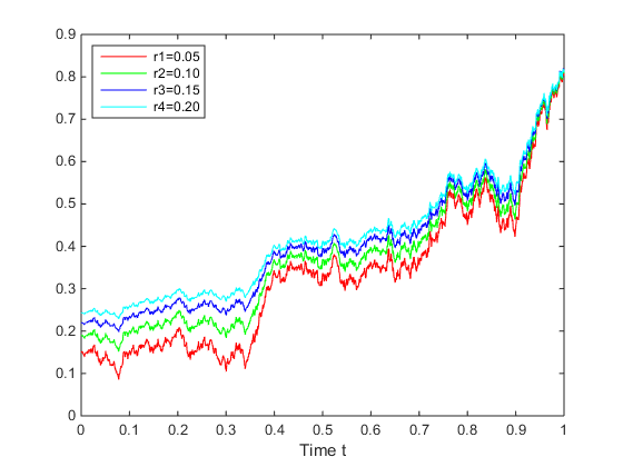
Figure 1: The relationship between $r$ and $u^{*}_{t}$.

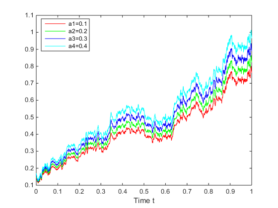
Figure 2: The relationship between $a$ and $u^{*}_{t}$.

A.: The relationship between $r$ and $u^{*}_{t}$.
Let $a_{t}=0.2$, $[r_{1t},r_{2t},r_{3t},r_{4t}]=[0.05,0.1,0.15,0.2]$. We plot Fig. 5.1 which illustrates the relationship between the optimal investment strategy $u^{*}_{t}$ and the risk-free rate $r_{t}$. From Fig. 5.1, we find that the higher the risk-free rate is, the higher the amount of investor’s wealth allocated in the stock share is. It is reasonable that the net wealth expectation $\mathbb{E}[I_{t}]$ increases with the increase of the risk-free rate, which leads to the increase of the liability $L_{t}$. Thus, the investor has to invest more in stock share to avoid the risk of the net wealth.

B: The relationship between $a$ and $u^{*}_{t}$.
Let $r_{t}=0.05$, $[a_{1t},a_{2t},a_{3t},a_{4t}]=[0.1,0.2,0.3,0.4]$. We plot Fig. 5.2 which illustrates the relationship between the optimal investment strategy $u^{*}_{t}$ and the appreciation rate of the liability $a_{t}$. Fig. 5.2 shows that the higher the appreciation rate of the liability is, the higher the amount of investor’s wealth allocated in the stock share is. It is reasonable that the liability increases with the increase of the appreciation rate of liability. Consequently, the investor has to invest more in stock share to avoid the risk of the net wealth.

6 Concluding remarks

We use an equivalent cost functional method to deal with an indefinite MF-LQJ problem. Relying on this method, we transform an indefinite MF-LQJ problem to a definite MF-LQJ problem. Compared with existing literature, we further consider the unique solvabilities of Riccati equations arising in indefinite MF-LQJ problems, which have not been studied before. Moreover, the method provides an alternative approach to solve MF-FBSDEJ. Several illustrative examples show that our method is more effective than existing methods in proving the existence and uniqueness of solution to MF-FBSDEJ. Our results are obtained with the framework of MF-LQJ problem. We will further investigate some results for other stochastic system. For example, LQ optimal control with delay has not been completely solved yet. We will try to extend this method to the framework with delay.

References

- [1] D. Andersson and B. Djehiche, “A maximum principle for SDEs of mean-field type,” Appl. Math. Optim., vol. 63, no. 3, pp. 341-356, 2011.
- [2] J. Barreiro-Gomez, T. E. Duncan, and H. Tembine, “Discrete-time linear-quadratic mean-field-type repeated games: perfect, incomplete, and imperfect information,” Automatica, vol. 112, 2020, Art. no. 108647.
- [3] J. Barreiro-Gomez, T. E. Duncan, and H. Tembine, “Linear-quadratic mean-field-type games: jump-diffusion process with regime switching,” IEEE Trans. Autom. Control, vol. 64, no. 10, pp. 4329-4336, 2019.
- [4] A. Bensoussan, S. C. P. Yam, and Z. Zhang, “Well-posedness of mean-field type forward-backward stochastic differential equations,” Stochastic Process. Appl., vol. 125, no. 9, pp. 3327-3354, 2015.
- [5] R. Buckdahn, J. Li, and J. Ma, “A stochastic maximum principle for general mean-field systems,” Appl. Math. Optim., vol. 74, no. 3, pp. 507-534, 2016.
- [6] R. Carmona and F. Delarue, “Mean-field forward-backward stochastic diffierential equations,” Electron. Commun. Probab., vol. 18, no. 68, pp. 1-15, 2013.
- [7] R. Carmona and F. Delarue, “Probabilistic analysis of mean-field games,” SIAM J. Control Optim., vol. 51, no. 4, pp. 2705-2734, 2013.
- [8] R. Carmona and F. Delarue, “Forward-backward stochastic diffierential equations and controlled mckean-vlasov dynamics,” Ann. Probab., vol. 43, no. 5, pp. 2647-2700, 2015.
- [9] S. Chen, X. Li, and X. Zhou, “Stochastic linear quadratic regulators with indefinite control weight costs,” SIAM J. Control Optim., vol. 36, no. 5, pp. 1685-1702, 1998.
- [10] S. Chen and X. Zhou, “Stochastic linear quadratic regulators with indefinite control weight costs. ii,” SIAM J. Control Optim., vol. 39, no. 4, pp. 1065-1081, 2000.
- [11] M. C. Chiu and D. Li, “Asset and liability management under a continuoustime mean-variance optimization framework,” Insurance Math. Econom., vol. 39, no. 3, pp. 330-355, 2006.
- [12] B. Djehiche, H. Tembine, and R. Tempone, “A stochastic maximum principle for risk-sensitive mean-field type control,” IEEE Trans. Autom. Control, vol. 60, no. 10, pp. 2640-2649, 2015.
- [13] R. Elliott, X. Li, and Y. Ni, “Discrete time mean-field stochastic linear-quadratic optimal control problems,” Automatica, vol. 49, no. 11, pp. 3222-3233, 2013.
- [14] S. Haadem, B. Øksendal, and F. Proske, “Maximum principles for jump diffusion processes with infinite horizon,” Automatica, vol. 49, no. 7, pp. 2267-2275, 2013.
- [15] J. Huang and Z. Yu, “Solvability of indefinite stochastic riccati equations and linear quadratic optimal control problems,” Syst. Control Lett., vol. 68, pp. 68-75, 2014.
- [16] N. Li, X. Li, and Z. Yu, “Indefinite mean-field type linear-quadratic stochastic optimal control problems,” Automatica, vol. 122, 2020, Art. no. 109627.
- [17] W. Li and H. Min, “Fully coupled mean-field FBSDEs with jumps and related optimal control problems,” Optim. Control Appl. Meth., vol. 42, no. 1, pp. 305-329, 2021.
- [18] X. Li, J. Sun, and J. Yong, “Mean-field stochastic linear quadratic optimal control problems: closed-loop solvability,” Probab. Uncertain. Quant. Risk, vol. 1, 2016, Art. no. 2.
- [19] Y. Ni, X. Li, and J. Zhang, “Indefinite mean-field stochastic linearquadratic optimal control: from finite horizon to infinite horizon,” IEEE Trans. Autom. Control, vol. 61, no. 11, pp. 3269-3284, 2015.
- [20] Y. Ni, J. Zhang, and X. Li, “Indefinite mean-field stochastic linear quadratic optimal control,” IEEE Trans. Autom. Control, vol. 60, no. 7, pp. 1786-1800, 2014.
- [21] B. Øksendal and A. Sulem, “Applied stochastic control of jump diffusions.” Springer-Verlag, New York, 2007.
- [22] Q. Qi, H. Zhang, and Z. Wu, “Stabilization control for linear continuous-time mean-field systems,” IEEE Trans. Autom. Control, vol. 64, no. 8, pp. 3461-3468, 2019.
- [23] Y. Shen, Q. Meng, and P. Shi, “Maximum principle for mean-field jump-diffusion stochastic delay differential equations and its application to finance,” Automatica, vol. 50, no. 6, pp. 1565-1579, 2014.
- [24] J. Sun, “Mean-field stochastic linear quadratic optimal control problems: open-loop solvabilities,” ESAIM Control Optim. Calc. Var., vol. 23, no. 3, pp. 1099-1127, 2017.
- [25] C. Tang , X. Li, and T. Huang, “Solvability for indefinite mean-field stochastic linear quadratic optimal control with random jumps and its applications,” Optim. Control Appl. Meth., vol. 41, no. 6, pp. 2320-2348, 2020.
- [26] M. Tang and Q. Meng, “Linear-quadratic optimal control problems for mean-field stochastic diffierential equations with jumps,” Asian J. Control, vol. 21, no. 2, pp. 809-823, 2019.
- [27] B. Wang, H. Zhang, and J. Zhang, “Mean field linear-quadratic control: uniform stabilization and social optimality,” Automatica, vol. 121, 2020, Art no. 109088.
- [28] G. Wang, C. Zhang, and W. Zhang, “Stochastic maximum principle for mean-field type optimal control under partial information,” IEEE Trans. Autom. Control, vol. 59, no. 2, pp. 522-528, 2014.
- [29] G. Wang, H. Xiao, and G. Xing, “An optimal control problem for mean-field forward-backward stochastic differential equation with noisy observation,” Automatica, vol. 86, pp. 104-109, 2017.
- [30] J. Wei and T. Wang, “Time-consistent mean-variance asset-liability management with random coefficients,” Insurance Math. Econom., vol. 77, pp. 84-96, 2017.
- [31] J. Yong, “Linear-quadratic optimal control problems for mean-field stochastic diffierential equations,” SIAM J. Control Optim., vol. 51, no. 4, pp. 2809-2838, 2013.
- [32] Z. Yu, “Equivalent cost functionals and stochastic linear quadratic optimal control problems,” ESAIM Control Optim. Calc. Var., vol. 19, no. 1, pp. 78-90, 2013.