HARA: A Hierarchical Approach for Robust Rotation Averaging

Abstract

We propose a novel hierarchical approach for multiple rotation averaging, dubbed HARA. Our method incrementally initializes the rotation graph based on a hierarchy of triplet support. The key idea is to build a spanning tree by prioritizing the edges with many strong triplet supports and gradually adding those with weaker and fewer supports. This reduces the risk of adding outliers in the spanning tree. As a result, we obtain a robust initial solution that enables us to filter outliers prior to nonlinear optimization. With minimal modification, our approach can also integrate the knowledge of the number of valid 2D-2D correspondences. We perform extensive evaluations on both synthetic and real datasets, demonstrating state-of-the-art results.

1 Introduction

We consider the problem of multiple rotation averaging in the presence of outliers, i.e., finding multiple absolute rotations $\mathbf{R}_{i}$ given a partial set of noisy, outlier-contaminated constraints on relative rotations $\mathbf{R}_{ij}=\mathbf{R}_{i}\mathbf{R}_{j}^{\top}$ [35]. This problem has direct application to structure-from-motion (SfM) [44, 20, 1, 47, 62, 17, 18, 67, 15, 13, 65], multiple point cloud registration [32, 56, 4, 3, 36, 5, 28, 46] and simultaneous localization and mapping (SLAM) [10, 8, 7, 66].

In most global SfM pipelines, multiple rotation averaging is the de facto standard for computing the initial orientations of the cameras: After estimating the relative poses between image pairs (e.g., by matching feature descriptors such as SIFT [43] and running the 5-point algorithm [48] with RANSAC [23]), one can solve the rotation averaging problem and obtain the absolute rotations with respect to a common reference frame. These initial rotations are then used in subsequent operations such as translation estimation [62, 17], pose graph optimization [10, 46], multiview triangulation [38, 41] and bundle adjustment [57, 34, 42]. As a result, all these tasks depend critically on the solution produced by the rotation averaging algorithm.

For this reason, numerous research endeavors have been made in the past decade to develop reliable and versatile rotation averaging methods. However, even without any outliers in the input, solving a large-scale rotation averaging problem is nontrivial [61, 60]. The problem only gets worse when the input contains outliers, which is often the case in practice [62, 12, 46]. These outliers, if not handled properly, can easily degrade the estimation accuracy.

Commonly, rotation averaging is formulated as a nonlinear optimization problem and solved iteratively starting from some initial guess of the absolute rotations [33, 12, 54, 13]. If, however, this initial guess is severely affected by outliers, it becomes extremely difficult to obtain an accurate result later on. Therefore, a robust initialization is essential for reliable rotation averaging in the presence of outliers.

In this work, we propose a novel method for robust multiple rotation averaging. Our main contribution is a hierarchical initialization scheme that constructs a spanning tree of a rotation graph by propagating most reliable constraints first and less reliable ones later. We establish the hierarchy of reliability based on the number of consistent triplet constraints, as well as their level of consistency. That is, we consider a constraint to be more reliable if it is strongly supported by many other constraints and less reliable if it has weaker or fewer supports. Optionally, we can also incorporate the number of valid 2D-2D correspondences into the hierarchy. Experimental results show that our approach can significantly improve the robustness of rotation averaging. To download our code and the supplementary material, go to https://seonghun-lee.github.io.

2 Related Work

Early works on motion averaging demonstrated various methods for estimating absolute rotations from pairwise constraints [29, 52, 25, 30, 44]. In recent works, the focus has been on either (1) achieving the global optimality in the absence of outliers, or (2) obtaining a robust solution in the presence of outliers. This work belongs to the second group.

(1) Globally optimal methods in outlier-free scenarios:
In [24, 9], globally optimal methods using Lagrangian duality are proposed. In later works, more advanced optimization methods have been proposed to enhance the speed and scalability, while guaranteeing the global optimality of the solution [21, 22, 51]. For more recent works on optimal methods, we refer to [19, 49, 45].

(2) Robust methods in the presence of outliers:
Various methods have been proposed to handle outliers (see [58] for a survey). First, there are methods that attempt to detect and remove outliers, e.g., [31, 64, 14]. Govindu [31] uses a RANSAC-based method by sampling random spanning trees. Zach et al. [64] employ a more tractable approach based on Bayesian inference from sampled loop inconsistencies. In [14], Crandall et al. use discrete belief propagation on a Markov random field to obtain the initial solution and remove edges with large errors.

On the other hand, some methods do not completely remove outliers, but instead suppress large errors during optimization. For example, Hartley et al. [33] apply single rotation averaging under the $L_{1}$ norm to update each absolute rotation in a distributed manner. Wang and Singer [59] use semidefinite relaxation and an alternating direction method to minimize a cost function based on the $L_{1}$ norm. Chatterjee and Govindu [11, 12] apply the Lie-algebraic averaging [30] using the iteratively reweighted least squares (IRLS) method with a robust loss function. In [3], Arrigoni et al. demonstrate that the spectral decomposition method in [1] can be robustified using the IRLS method. Recently, Shi and Lerman [54] proposed an alternative optimization method, called message passing least squares, and demonstrated its advantages over the IRLS approach [12].

Other robust methods directly model the presence of outliers in the optimization problem: Boumal et al. [6] take into account the outliers in the noise model and compute the maximum likelihood estimate via Riemannian trust-region optimization. Arrigoni et al. [2, 3] intrinsically include the outliers in the cost function and estimate the rotations via low-rank and sparse matrix decomposition.

Another popular approach is to exploit additional visual information (e.g., the number of inlier feature matches or the similarity score) to identify inlier edges and obtain a robust initial solution [20, 53, 16, 13, 26, 27].

Recently, learning-based approaches have been proposed in [50, 63]. Although these supervised methods may not always generalize well to unfamiliar settings, they show impressive performance on data similar to the training data.

3 Preliminaries and Notation

We denote the Euclidean and the Frobenius norm of a 3D vector $\mathbf{v}$ by $\lVert\mathbf{v}\rVert$ and $\lVert\mathbf{v}\rVert_{F}$, respectively. We represent a rotation with a rotation matrix $\mathbf{R}\in SO(3)$ or a rotation vector $\mathbf{u}=\theta\widehat{\mathbf{u}}$ where $\theta$ and $\widehat{\mathbf{u}}$ are the angle and the unit axis of the rotation, respectively. The two representations are related by Rodrigues’ formula, and we denote the mapping between them by $\text{Exp}(\cdot)$ and $\text{Log}(\cdot)$ [55]:

$$\mathbf{R}=\mathrm{Exp}(\mathbf{u}),\quad\mathbf{u}=\mathrm{Log}(\mathbf{R}).$$ (1)

In the context of SfM, the absolute rotation and translation of camera $i$ are denoted as $\mathbf{R}_{i}$ and $\mathbf{t}_{i}$, respectively. Together, they transform a 3D point from the world frame to the camera reference frame: $\mathbf{x}_{i}=\mathbf{R}_{i}\mathbf{x}_{w}+\mathbf{t}_{i}$. We denote with $\mathbf{R}_{jk}$ the relative rotation between $\mathbf{R}_{j}$ and $\mathbf{R}_{k}$, i.e., $\mathbf{R}_{jk}=\mathbf{R}_{j}\mathbf{R}_{k}^{\top}$.

The angular distance between $\mathbf{R}_{j}$ and $\mathbf{R}_{k}$ is defined as the angle of the rotation $\mathbf{R}_{j}\mathbf{R}_{k}^{\top}$, i.e.,

$$d(\mathbf{R}_{j},\mathbf{R}_{k})=\lVert\mathrm{Log}\left(\mathbf{R}_{j}\mathbf{R}_{k}^{\top}\right)\rVert.$$ (2)

The chordal distance is related to the angular distance by the following equation [35]:

$$d_{\text{chord}}(\mathbf{R}_{j},\mathbf{R}_{k}):= \lVert\mathbf{R}_{j}-\mathbf{R}_{k}\rVert_{F}$$ (3)

$$= 2\sqrt{2}\sin{\left(d(\mathbf{R}_{j},\mathbf{R}_{k})/2\right)}.$$ (4)

If both $\mathbf{R}_{j}$ and $\mathbf{R}_{k}$ have a small angle, their relative rotation can be approximated using the Baker-Campbell-Hausdorff (BCH) formula [30]:

$$\mathbf{R}_{j}\mathbf{R}_{k}^{\top}\approx\mathrm{Exp}(\mathbf{u}_{j}-\mathbf{u}_{k}).$$ (5)

$$\Rightarrow\ \mathrm{Log}\left(\mathbf{R}_{j}\mathbf{R}_{k}^{\top}\right)\approx\mathbf{u}_{j}-\mathbf{u}_{k}.$$ (6)

In the following, we list some important terminology:

• Nodes and edges: Multiple absolute rotations are related to each other in pairs, so the underlying structure can be represented by a graph. In this context, the nodes represent the unknown absolute rotations, and the edges represent the known pairwise constraints.

• Neighbors: When two nodes are connected by an edge, they are each other’s neighbors.

• Fixed nodes and family: Once a node is initialized with some absolute rotation, we call it fixed. A family refers to the set of all fixed nodes. The goal of the initialization is to have all nodes included in the family.

• Base node: One of the fixed nodes can be chosen as the base node at any time during the initialization. This is the node from which the yet-incomplete spanning tree will branch out if a certain condition is met.

• Consistent triplet: Node $i$, $j$ and $k$ form a consistent triplet if and only if the input relative rotations satisfy

  $$d_{\text{chord}}(\mathbf{R}_{ij}^{\text{in}},\mathbf{R}_{ik}^{\text{in}}\mathbf{R}_{kj}^{\text{in}})<\epsilon,$$ (7)

  where $\epsilon$ is called a loop threshold. A triplet that satisfies Eq. (7) under small $\epsilon$ is described as “strong”, and one that does it under relatively large $\epsilon$ is described as “weak”. If a triplet contains one or more outlier edges, it is most likely to be inconsistent and fail to meet Eq. (7).

• Number of triplet supports: Suppose that a base node has several non-family neighbors, including node $i$. The number of triplet supports of neighbor $i$ refers to the number of consistent triplets formed by the base node, node $i$ and another neighbor of the base node. A simple example is illustrated in Fig. 1.

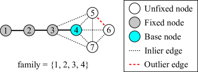
Figure 1: In this example, the base node (4) has three non-family neighbors (5, 6 and 7). We check the triplet consistency (Eq. (7)) without directly inferring the outlier edge: Node 5 has two triplet supports, i.e., (3, 4, 5) and (4, 5, 7), 6 has one support, i.e., (4, 6, 7), and 7 has three supports, i.e., (3, 4, 7), (4, 5, 7) and (4, 6, 7).

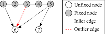
Figure 2: Here, no matter which family member is chosen as the base node, we cannot form a consistent triplet. In this case, we let every family member vote for their non-family neighbors and add the one with the most votes (node 6) to the family. Among the candidate rotations propagated from node 1, 3 and 5, we choose the one that is closest to their robust average (obtained using [40]).

1 $s\leftarrow s_{\scaleto{\text{init}}{5pt}}$, $\texttt{family}\leftarrow\{\}$, $\texttt{newFamily}\leftarrow\{\}$;

2 Add the node with the most neighbors to family and newFamily, and set its rotation to identity;

3 while not all nodes are in family do

4       while newFamily is not empty do

5             Choose a member of newFamily as the base node and remove it from newFamily;

6             Propagate away from the base node to its non-family neighbors using Eq. (8), and add those with $s$ or more triplet supports to family and newFamily;

7             if at least one node is added to newFamily then

8                   $s\leftarrow s_{\scaleto{\text{init}}{5pt}}$;

9                  

10             end if

11            

12       end while

13      For the next base node, choose the family member that has the most non-family neighbors with $s$ or more supports;

14       if the base node has at least one non-family neighbor with $s$ or more supports then

15             Add the base node to newFamily.

16      else

17             $s\leftarrow s-1$;

18            

19       end if

20      

21      if $s=0$ then

22             Let every family member vote for their non-family neighbors, add the one with the most votes to family and newFamily, and set its rotation via single rotation averaging (see Fig. 2);

23             $s\leftarrow s_{\scaleto{\text{init}}{5pt}}$;

24            

25       end if

26      

27 end while

Algorithm 1 Hierarchical Initialization (simplified)

4 Method

The proposed method consists of three steps:

1. Robust initialization of the absolute rotations by building a spanning tree in a hierarchical manner. If the number of inlier matches is known for all edges, we can optionally incorporate it in the initialization.

2. Filtering the edges that do not conform to the initial solution to remove as many outliers as possible.

3. Iterative local refinement using nonlinear optimization.

To make the initialization step easier to understand, we first describe the simplified version in Section 4.1 and then the full version in Section 4.2. We explain the edge filtering and the local refinement in Section 4.3 and 4.4, respectively.

4.1 Hierarchical initialization (simplified version)

We initialize the absolute rotations by constructing a spanning tree of the graph. As we expand the tree incrementally, we want to avoid as many outlier edges as possible, so we start adding the most reliable edges first. In our method, there are two modes of tree expansion: (1) based on the triplet support, or (2) via single rotation averaging.

First, we set a certain integer threshold $s$ (called a support threshold) and check if the base node has any non-family neighbors with $s$ or more triplet supports. If so, we add these neighbors to the family and obtain their rotations $(\mathbf{R}_{\text{N}}^{\text{est}})$ by propagating from the base node $(\mathbf{R}_{\text{B}}^{\text{est}})$, i.e.,

$$\mathbf{R}_{\text{N}}^{\text{est}}\leftarrow\mathbf{R}_{\text{NB}}^{\text{in}}\mathbf{R}_{\text{B}}^{\text{est}}.$$ (8)

For example, if $s$ = 2 in Fig. 1, we would add node 5 and 7 in the family, but not 6. If all non-family neighbors of the family have fewer than $s$ triplet supports, we update $s\leftarrow s-1$ and, for the next base node, choose the family member that has the most non-family neighbors with $s$ or more supports. We repeat the same propagation process afterwards.

Another way to expand the tree is to add a node via single rotation averaging when all non-family neighbors of the family have zero triplet support. In this case, we let every family member vote for their non-family neighbors, and the one with the most votes is added to the family. This node also becomes the next base. To determine its rotation, we first obtain the candidate rotations by propagating from the family nodes that voted for it. Then, we average these rotations using the robust single rotation averaging method in [40]. Finally, the candidate rotation that is closest to the result is assigned to the node. Fig. 2 shows an example.

At each iteration, our initialization algorithm decides between the two aforementioned modes of tree expansion. We first try expanding based on the triplet support by adapting the support threshold $s$, and when $s=0$, we expand the tree via voting and single rotation averaging. Every time a node is added to the family, we reset $s$ to the initial value. Alg. 1 summarizes the procedure and Fig. 3 shows a toy example.

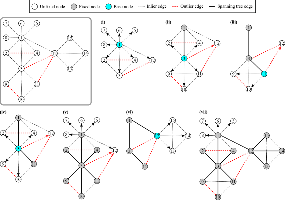
Figure 3: [Top left] A toy example. We show the steps of our initialization algorithm with $s=2$ and a fixed loop threshold.
aaa(i) First, we choose the node with the most neighbors (node 1) as the base node and set its rotation to identity. This node is the first member of the family. By propagating away from this node using Eq. (8), its neighbors get tentative rotations. For each neighbor, we count the number of triplet supports (i.e., the number of other neighbors supporting it), and if it has $s$ or more supports, we add it to the family. In this example, node 3 is supported by two other neighbors (node 2 and 4), and it is the only one added to the family. Node 3 becomes the next base node, and we fix its rotation. Also, the edge (1, 3) turns into a spanning tree edge.
aaa(ii) We repeat the same process by propagating away from the new base node (node 3). The only non-family neighbor that has $s$ or more supports is node 11, so we fix its rotation, add it to the family, and select it as the next base node.
aaa(iii) We propagate away from the new base node (node 11), but no neighbor has enough supports. In this case, we update $s\leftarrow s-1$ and check for each family member how many neighbors have $s$ or more supports: node 1 has two (node 2 and 4), node 3 has four (node 2, 4, 9, 10), and node 11 has two (node 9 and 10). Since node 3 has the most, it becomes the next base node. Note that in the full version of the algorithm, we do this counting as soon as the base node changes and store the results for reuse (more details in Section 4.2).
aaa(iv) We propagate away from the new base node (node 3), and the non-family neighbors with $s$ (= 1) supports are node 2, 4, 9 and 10. These four nodes are added to the family, and their rotations are fixed.
aaa(v) With node 1–4 and 9–11 in the family, none of their non-family neighbors has a single support. In this case, each family member votes for their non-family neighbors, and the one with the most votes is added to the family. This node (node 12) also becomes the next base node. To determine its rotation, we first average the candidate rotations propagated from node 1, 3 and 11 using [40]. Then, the candidate rotation that is closest to the result is assigned to node 12, and the corresponding edge becomes a spanning tree edge. In this example, let us suppose that it is the edge (1, 12).
aaa(vi) Every time a node is added to the family, we reset $s$ to the initial value ($s\leftarrow 2$). Afterwards, we repeat the process of propagating away from the base node and adding the neighbors with $s$ or more supports to the family. In this example, node 12 has three non-family neighbors (node 13, 14, 15) and they all have $s$ supports. Therefore, all three of them are added to the family and their rotations are fixed.
aaa(vii) With node 1–4 and 9–13 in the family, none of their non-family neighbors has $s$ (= 2) supports. We update $s\leftarrow s-1$ and check again, but none has a single support. Now, as in Step (v), we let every family member vote for their non-family neighbors, and add the one with the most votes. Repeating this procedure adds node 5–8 to the family one by one. Finally, all nodes are in the family and their rotations are fixed. The algorithm returns the estimated rotations of all nodes.

1 $s\leftarrow s_{\scaleto{\text{init}}{5pt}}$, $\texttt{family}\leftarrow\{\}$, $\texttt{newFamily}\leftarrow\{\}$;

2 Add the node with the most neighbors to family and newFamily, and set its rotation to identity;

3

4Determine the loop thresholds $\epsilon_{1}$, $\epsilon_{2}$, …, $\epsilon_{m}$;

5

6$i\leftarrow 1,\ \epsilon\leftarrow\epsilon_{\scaleto{i}{5pt}}$;

7

8$\texttt{snTable}\leftarrow\text{Zero 3D array of dimension }n\times m\times s$;

9

($n$ is #nodes, $m$ is #loop thresholds, $s$ is a support threshold)

10while not all nodes are in family do

11       while newFamily is not empty do

12             Choose a member of newFamily as the base node and remove it from newFamily;

13             Propagate away from the base node to its non-family neighbors using Eq. (8) and add those with $s$ or more triplet supports to family and newFamily;

14            

15            Update snTable for the base node;

16            

17            if at least one node is added to newFamily then

18                   $s\leftarrow s_{\scaleto{\text{init}}{5pt}}$, $i\leftarrow 1,\ \epsilon\leftarrow\epsilon_{\scaleto{i}{5pt}}$;

19                  

20             end if

21            

22       end while

23      In snTable, find the family member that has the most non-family neighbors with $s$ or more triplet supports under the current threshold $\epsilon$. Choose it as the base node;

24      

25      if the base node has at least one non-family neighbor with $s$ or more supports then

26             Add the base node to newFamily.

27      else

28            

29            if $i<m$ then

30                   $i\leftarrow i+1,\ \epsilon\leftarrow\epsilon_{\scaleto{i}{5pt}}$;

31                  

32            else

33                   $s\leftarrow s-1,\ i\leftarrow 1,\ \epsilon\leftarrow\epsilon_{\scaleto{i}{5pt}}$;

34                  

35             end if

36            

37       end if

38      

39      if $s=0$ then

40             Let every family member vote for their non-family neighbors, add the one with the most votes to family and newFamily, and set its rotation via single rotation averaging (see Fig. 2);

41             $s\leftarrow s_{\scaleto{\text{init}}{5pt}}$, $i\leftarrow 1,\ \epsilon\leftarrow\epsilon_{\scaleto{i}{5pt}}$;

42            

43       end if

44      

45 end while

Algorithm 2 Hierarchical Initialization (full version)

4.2 Hierarchical initialization (full version)

The simplified algorithm described in the previous section constructs a spanning tree by adding the most supported edges first. In the full version, we consider two more aspects: the loop threshold $\epsilon$ in Eq. (7), and optionally, the number of valid 2D-2D correspondences. We highlight the differences between the two versions in Alg. 2.

In the simplified version, the consistency of a triplet depends entirely on a single threshold $\epsilon$ we set. In the full version, we set multiple thresholds ($\epsilon_{1}$, $\epsilon_{2}$, …, $\epsilon_{m}$ in ascending order) and adaptively switch between them. Specifically, we start from the smallest (the strictest) threshold and gradually move on to larger (less strict) thresholds. As a result, the following hierarchy is established:

1. Neighbor nodes with many triplet supports under small $\epsilon_{i}$ are added to the family first.

2. Those with many supports under large $\epsilon_{i}$ are added next.

3. Those with few supports under small $\epsilon_{i}$ are added next.

4. Those with few supports under large $\epsilon_{i}$ are added last.

Another change from the simplified version is that we store the number of supported neighbors each time we try propagating away from the base node. This data is stored in a supported neighbors table (SN table), a 3D array whose dimensions correspond to the base node index, the threshold index, and the number of triplet supports. We organize this table such that the entry at position ($x$, $y$, $z$) corresponds to the number of non-family neighbors of base node $x$ that have $z$ or more supports under the $y$-th threshold $\epsilon_{y}$. Note that each time we update the SN table for the current base node, we update it for all $y=1,2,\dots,m$ and $z=1,2,\dots,s_{\scaleto{\text{init}}{5pt}}$. This is done in line 2 of Alg. 2.

The advantage of maintaining this table is that we can reuse it to promptly find the node with the most number of supported neighbors for any given $s$ and $\epsilon$ (line 2 of Alg. 2). This operation is necessary when we have to choose the next base node after $s$ is decremented. Although the data in the SN table may sometimes be outdated (because some non-family neighbors can turn into family members later), we can at least avoid having to evaluate the neighbors of all family members repeatedly (i.e., line 1 of Alg. 1).

Our approach can also seamlessly integrate the knowledge of the number of valid 2D-2D correspondences. This can be done with minimal modification of Alg. 2: Let $d_{1}$, $d_{2}$, …, $d_{k}$ (in descending order) be some thresholds we set for the number of valid 2D-2D correspondences. Then, we run the outer loop (line 2–2) while pretending that all edges whose valid correspondences are fewer than $d_{1}$ do not exist. When the number of total votes becomes zero in line 2, we reset $s$, $\epsilon$ and the SN table to the initial state, switch the correspondence threshold to the next one ($d_{2}$) and continue. This process ensures that the edges with very few valid correspondences are added last.

Implementation details:

1. In line 1 of Alg. 1 and line 2 of Alg. 2, if newFamily has multiple members, we choose the one with the most neighbors as the base node. This is because we want to add well-connected nodes first to minimize drift.

2. In all of our experiments in this paper, we fix $s_{\scaleto{\text{init}}{5pt}}=10$, $d_{1}=5$ and $d_{2}=0$.

3. For good performance, the loop thresholds should reflect the noise level of the inlier edges. To this end, we use a simple heuristic method to determine their values in line 2 of Alg. 2: For each edge $(i,j)$, we sample at most 10 common neighbors of node $i$ and $j$, forming up to 10 triplets $(i,j,k)$. We compute the loop errors (7) of all triplets from all edges and collect only those below $1$. Then, we set the loop thresholds $\epsilon_{1}$, $\epsilon_{2}$ and $\epsilon_{3}$ to the 10th, 20th and 30th percentile of the collected errors.

4.3 Edge filtering

Having obtained an initial solution $(\mathbf{R}_{i}^{\text{est}}$ for $i$ = 1, 2, $\dots,n)$ from the spanning tree in Section 4.2, we next filter potential outlier edges in the full rotation graph before optimizing the solution. This is done by checking whether or not each edge conforms to the initial solution. Specifically, we consider edge $(j,k)$ as an outlier and exclude it from the further operations if the following condition is met:

$$d_{\text{chord}}\left(\mathbf{R}_{jk}^{\text{in}},\mathbf{R}_{j}^{\text{est}}{\mathbf{R}_{k}^{\text{est}}}^{\top}\right)>\tau,$$ (9)

where $\tau$ is some threshold (we set $\tau=1$ in this work).

While this filtering step often enhances the robustness for moderate outlier ratios ($<0.3$), we found that it sometimes worsens the accuracy for higher outlier ratios. Therefore, we skip this step when we deem the outlier ratio to be too high. In practice, we assume that this is the case when the median of the loop errors from all sampled triplets is larger than $1$ (see the implementation detail 3 of Section 4.2).

4.4 Local refinement

Given the initial solution and the filtered constraints $(\mathbf{R}_{jk}^{\text{in}}\text{ for }(j,k)\in\text{ filtered edges})$, we perform an iterative local refinement using the optimization method proposed in [12]. In the following, we briefly summarize this method.

The goal here is to find the optimal updates such that the updated solution fits the constraints better, i.e.,

$$\mathbf{R}_{jk}^{\text{in}}=\left(\mathbf{R}_{j}^{\text{est}}\Delta\mathbf{R}_{j}\right)\left(\mathbf{R}_{k}^{\text{est}}\Delta\mathbf{R}_{k}\right)^{\top}.$$ (10)

Rearranging this and taking the $\mathrm{Log}$ (1) of both sides gives

$$\mathrm{Log}\left(\mathbf{R}_{j}^{\text{est}\top}\mathbf{R}_{jk}^{\text{in}}\mathbf{R}_{k}^{\text{est}}\right)=\mathrm{Log}\left(\Delta\mathbf{R}_{j}\Delta\mathbf{R}_{k}^{\top}\right).$$ (11)

Assuming that the updates are small, we can use the approximation in Eq. (6) on the right-hand side and obtain

$$\mathrm{Log}\left(\mathbf{R}_{j}^{\text{est}\top}\mathbf{R}_{jk}^{\text{in}}\mathbf{R}_{k}^{\text{est}}\right)\approx\Delta\mathbf{u}_{j}-\Delta\mathbf{u}_{k},$$ (12)

where $\Delta\mathbf{u}_{j}$ and $\Delta\mathbf{u}_{k}$ are the rotation vectors of $\Delta\mathbf{R}_{j}$ and $\Delta\mathbf{R}_{k}$, respectively. Since the left-hand side of Eq. (12) is known, stacking these equations for all filtered edges results in a linear system of equations, which we solve using a linear algebra library. We update the rotations, i.e., $\mathbf{R}_{i}^{\text{est}}\leftarrow\mathbf{R}_{i}^{\text{est}}\Delta\mathbf{R}_{i}$ for all $i$, plug them back into Eq. (12) and repeat the same process until convergence. In practice, we carry out the optimization using the IRLS method with the $\ell_{\frac{1}{2}}$ loss function, as in [12]. Also, to reduce the total number of arithmetic operations, all rotations (both absolute and relative) are parameterized as quaternions. For more details, we refer to the original work [12].

5 Results

We compare our method with the following methods: R-GoDec [2, 3], Eig-IRLS [3], IRLS-$\ell_{\frac{1}{2}}$ [12], MPLS [54] and Hybrid RA [13]. Since the implementation of the view graph filtering (VGF) in Hybrid RA is not publicly available, we reproduced this part by ourselves. Note that this part is only applicable if 2D-2D correspondences are given for all edges. All methods are implemented in MATLAB, except Hybrid RA which is written in C++. We run all methods on a laptop with Intel’s 4th Gen i7 CPU (2.8 GHz).

We evaluate the accuracy using two error metrics:

$$\theta_{1} =\min_{\mathbf{R}_{\scaleto{\textrm{{align}}}{6pt}}}\frac{1}{n}\sum_{i=1}^{n}d\left(\mathbf{R}_{i}^{\text{gt}},\mathbf{R}_{i}^{\text{est}}\mathbf{R}_{\text{align}}\right),$$ (13)

$$\theta_{2} =\min_{\mathbf{R}_{\scaleto{\textrm{{align}}}{6pt}}}\sqrt{\frac{1}{n}\sum_{i=1}^{n}d\left(\mathbf{R}_{i}^{\text{gt}},\mathbf{R}_{i}^{\text{est}}\mathbf{R}_{\text{align}}\right)^{2}}.$$ (14)

They respectively represent the optimal mean and RMS error after aligning the estimated rotations to the ground truth. The rotation $\mathbf{R}_{\text{align}}$ in Eq. (13) and (14) can be obtained by solving the single rotation averaging problem under the $L_{1}$ and $L_{2}$ norm, respectively [33, 35].

5.1 Synthetic data

For a controlled study of various factors, we run Monte Carlo simulations in multiple settings: We generate $n$ random rotations in a circular order and obtain the relative rotation of $p$% of all possible pairs. The edges are established as follows: First, we connect all successive nodes (i.e. node 1&2, 2&3, …, $n$&1). Then, we connect those separated by one node (i.e. node 1&3, 2&4, …, $n-1$&1, $n$&2), and afterwards, those separated by two nodes, three nodes, and so forth. We continue this process until $p$% are connected in total. This leads to all nodes being connected to their local neighbors in a sliding window fashion. Next, we turn $q$% of the edges into outliers, i.e., random relative rotations. We exclude the edges between successive nodes, so that every node gets at least two inlier edges. Finally, all edges are perturbed by $\mathcal{N}(0,\sigma^{2})$ and their order is randomized. These edges are used as input to the rotation averaging algorithms. The simulation is configured by setting $\{n,\ p,\ q,\ \sigma\}$ to one of the following values: $n=\{100,200\}$ rotations, $p=\{50,20\}$%, $q=\{0,5,10,...,50\}$%, $\sigma=\{5,10\}$ deg. For each setting, we generate 100 independent datasets.

Fig. 4 and 5 present the results for 100 and 200 rotations, respectively. We see that MPLS and HARA are the two best performing methods, especially at high outlier ratios.

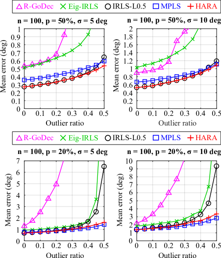
Figure 4: Simulation results (100 rotations): We plot the optimal mean errors, $\theta_{1}$ in Eq. (13). For dense graphs ($p=50$%), IRLS-$\ell_{\frac{1}{2}}$, MPLS and HARA perform similarly well. For sparse graphs ($p=20$%), MPLS and HARA are more robust to outliers than the rest, with MPLS being slightly better at high outlier ratios.

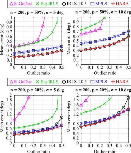
Figure 5: Simulation results (200 rotations): We plot the optimal mean errors, $\theta_{1}$ in Eq. (13). IRLS-$\ell_{\frac{1}{2}}$, MPLS and HARA perform similarly well, except that for sparse graphs ($p=20$%), IRLS-$\ell_{\frac{1}{2}}$ is outperformed by the other two at high outlier ratios.

5.2 Real data

Without using the number of inlier feature matches:
We evaluate the performance on the following real-world datasets: 1DSfM datasets [62], ‘Notre Dame 715’ (ND2) dataset³ [12], ‘Acropolis’ (ACP), ‘Arts Quad’ (ARQ) and ‘San Francisco’ (SNF) datasets [14]. As in [12], only those cameras whose ground truth is available are used to evaluate the accuracy, even though those without the ground truth are still included in the input for rotation averaging. Table 1 reports the results. It shows that in most cases HARA achieves state-of-the-art accuracy at a comparable speed.

Using the number of inlier feature matches:
For this experiment, we only use the 1DSfM dataset⁶ [62], as the other datasets do not provide the 2D-2D correspondences. The feature matches are only available for those cameras with the ground truth, so we disregard the rest. To check the validity of the correspondences, we put a threshold (0.01) on the sine of the $L_{1}$-optimal angular reprojection error [37, 39]. Table 2 presents the results. It shows that HARA achieves state-of-the-art results, with or without incorporating the number of inlier matches.

6 Limitations

The main limitation of our method is that it is sensitive to the parameters we set, especially the loop thresholds. Currently, we determine their values using a simple heuristic based on the sampled loop errors (Section 4.2). We noticed that, in some of the real datasets, a small change in this heuristic introduces a non-negligible fluctuation in the initialization accuracy. In future work, we plan to replace this heuristic with a more robust and reliable method.

7 Conclusion

We presented HARA, a hierarchical approach for robust multiple rotation averaging. For robust initialization of the rotation graph, we incrementally build a spanning tree based on a hierarchy of triplet support. That is, the edges supported by many strong triplets are added in the tree sooner than those with fewer or weaker triplets. This approach significantly reduces the influence of outliers on the initial solution, allowing us to filter outliers prior to nonlinear optimization. Also, we showed that we can optionally integrate the knowledge of the number of valid 2D-2D correspondences into our approach. An extensive evaluation demonstrates that HARA achieves state-of-the-art results.

Datasets				R-GoDec [3]			Eig-IRLS [3]			IRLS-$\ell_{\frac{1}{2}}$ [12]			MPLS∗ [54]			Hybrid RA [13]			HARA w/o
															w/o VGF$\hskip 1.0pt{}^{\bm{\dagger}}$			#inlier matches
Name	#views	%edges	$\theta_{1}$	$\theta_{2}$	Time	$\theta_{1}$	$\theta_{2}$	Time	$\theta_{1}$	$\theta_{2}$	Time	$\theta_{1}$	$\theta_{2}$	Time	$\theta_{1}$	$\theta_{2}$	Time	$\theta_{1}$	$\theta_{2}$	Time
ALM	627	49.5%	6.3	16.3	4s	3.9	12.2	21s	4.2	12.6	27s	3.7	12.1	29s	4.3	12.7	–	3.5	11.5	45s
ELS	247	66.8%	4.1	10.7	1s	3.3	11.5	3s	2.9	10.3	4s	2.8	10.9	7s	3.1	10.5	–	2.1	7.4	7s
GDM	742	17.5%	51.3	64.8	17s	65.8	74.2	29s	37.5	62.3	12s	40.7	68.7	74s	44.7	60.0	–	43.8	72.5	26s
MDR	394	30.7%	10.2	18.5	1s	10.9	22.4	5s	7.0	17.1	4s	5.2	14.7	5s	6.4	16.2	–	4.8	14.5	14s
MND	474	46.8%	6.2	18.4	3s	1.9	11.2	7s	1.5	7.4	10s	1.2	3.9	9s	1.5	6.9	–	1.1	2.1	20s
ND1	553	68.1%	5.2	15.5	6s	3.6	14.8	16s	3.5	14.6	28s	2.7	13.5	27s	3.5	14.7	–	1.6	6.3	55s
NYC	376	29.3%	6.4	9.9	6s	3.8	8.2	5s	3.0	7.0	3s	3.0	8.2	7s	3.2	7.4	–	2.9	7.7	10s
PDP	354	39.5%	11.4	22.0	2s	4.0	9.3	8s	4.1	8.1	4s	3.5	8.2	4s	5.3	10.4	–	3.4	7.4	9s
PIC	2508	10.2%	24.8	40.0	150s	81.0	91.2	687s	6.8	18.6	467s	4.6	14.6	295s	7.0	20.1	–	4.4	13.1	289s
ROF	1134	10.9%	12.6	19.5	61s	3.4	10.4	52s	3.1	10.2	12s	2.8	10.0	13s	3.1	9.2	–	2.7	8.5	31s
TOL	508	18.5%	6.4	13.1	8s	4.5	10.7	10s	3.9	9.0	2s	4.0	9.4	6s	4.4	10.5	–	4.3	10.0	13s
TFG	5433	4.6%	42.1	54.2	722s	59.4	67.1	833s	3.6	9.8	976s	4.5	10.8	1945s	15.1	17.8	–	3.5	10.7	925s
USQ	930	5.9%	12.0	23.7	27s	6.7	12.8	22s	9.3	22.2	10s	6.3	14.7	11s	9.3	21.7	–	6.0	12.3	9s
VNC	918	24.6%	16.1	36.9	25s	8.6	28.4	27s	8.3	27.5	28s	6.2	18.2	53s	8.4	27.2	–	6.1	18.1	47s
YKM	458	26.5%	6.1	11.3	7s	3.8	9.4	8s	3.5	8.4	3s	3.5	9.2	7s	3.5	8.4	–	3.0	6.9	16s
ND2	715	25.3%	2.7	10.0	10s	1.2	4.0	13s	1.1	3.5	13s	1.1	4.0	12s	1.1	3.5	–	1.3	5.5	23s
ACP	463	10.7%	0.8	1.2	6s	1.1	1.7	4s	1.2	1.7	1s	1.4	2.0	2s	1.2	1.7	–	1.2	1.7	7s
ARQ	5530	1.5%	29.7	56.5	1111s	70.1	79.7	4894s	4.0	7.1	173s	3.2	6.3	118s	3.9	6.9	–	3.6	6.8	137s
SNF	7866	0.3%	Out of memory			77.3	87.3	3.8h	3.6	4.2	180s	4.4	5.5	154s	4.3	6.2	–	3.6	4.2	44s
$\theta_{1}$ (deg): Optimal mean error in Eq. (13), $\theta_{2}$ (deg): Optimal RMS error in Eq. (14), $\text{\%edges}=\text{\#edges}/\text{\#possible pairs of views}$ in %.
∗Due to the non-deterministic nature of MPLS [54], we report the median of five independent runs.
†The computation times of Hybrid RA [13] are not included for comparison, since it is the only method implemented in C++.

Table 1: Results on the real datasets without the knowledge of the 2D-2D correspondences: For all datasets, HARA gives either better or comparable results to the state of the art. Interestingly, for the SNF dataset, it takes substantially less time than the rest. The results of MPLS [54] are mostly competitive with ours, except for the ELS, ND1, TFG and SNF datasets where HARA performs noticeably better. We run Hybrid RA [13] without view graph filtering because this requires the number of valid 2D-2D correspondences. As a result, this method does not provide much gain in accuracy compared to IRLS-$\ell_{\frac{1}{2}}$ [12], even though it performs an additional global optimization prior to local refinement. In fact, Hybrid RA performs much worse than IRLS-$\ell_{\frac{1}{2}}$ on the TFG dataset.

Datasets				IRLS-$\ell_{\frac{1}{2}}$ [12]			MPLS∗ [54]			Hybrid RA [13]			Hybrid RA [13]			HARA w/o			HARA with
									w/o VGF$\hskip 1.0pt{}^{\bm{\dagger}}$			with VGF$\hskip 1.0pt{}^{\bm{\dagger}}$			#inlier matches			#inlier matches
Name	#views	%edges	$\theta_{1}$	$\theta_{2}$	Time	$\theta_{1}$	$\theta_{2}$	Time	$\theta_{1}$	$\theta_{2}$	Time	$\theta_{1}$	$\theta_{2}$	Time	$\theta_{1}$	$\theta_{2}$	Time	$\theta_{1}$	$\theta_{2}$	Time
ALM	577	58.4%	4.0	12.4	28s	3.7	12.0	24s	4.3	12.8	–	3.0	10.2	–	3.5	11.5	41s	3.4	11.0	40s
ELS	227	78.0%	2.8	10.1	2s	3.0	11.7	6s	3.0	9.9	–	2.1	7.1	–	2.1	7.2	8s	1.8	4.8	6s
GDM	677	20.9%	37.4	62.2	8s	40.7	68.6	81s	34.5	55.3	–	39.9	68.7	–	44.1	72.5	23s	44.3	72.8	16s
MDR	341	40.7%	6.7	16.7	4s	5.1	14.4	4s	6.3	15.8	–	4.4	13.1	–	4.8	14.5	13s	4.8	14.8	11s
MND	450	51.8%	1.5	7.4	6s	1.2	3.9	8s	1.5	6.9	–	1.1	2.2	–	1.1	2.1	21s	1.1	2.1	18s
ND1	553	68.1%	3.5	14.6	29s	2.8	13.6	30s	3.5	14.7	–	1.7	6.1	–	1.6	6.3	61s	1.5	5.9	44s
NYC	332	37.4%	3.1	7.1	3s	3.1	8.2	7s	3.4	7.8	–	3.0	7.1	–	2.9	7.8	8s	2.6	5.8	7s
PDP	338	43.3%	4.1	8.2	4s	3.5	8.2	4s	5.2	10.3	–	3.1	6.4	–	3.5	7.8	8s	3.3	6.6	7s
PIC	2152	13.4%	6.2	17.0	419	4.7	14.6	254s	6.3	18.6	–	4.3	12.1	–	4.1	11.3	269s	4.0	11.3	247s
ROF	1084	11.9%	3.1	10.2	16s	2.8	9.7	13s	3.1	9.4	–	2.5	6.7	–	2.7	8.7	30s	2.5	7.6	25s
TOL	472	21.4%	3.9	8.9	2s	4.0	9.4	4s	4.4	10.4	–	4.0	9.4	–	4.3	10.0	8s	4.0	8.9	11s
TFG	5058	5.3%	3.5	8.9	881s	5.3	11.1	1466s	4.0	9.8	–	5.3	11.8	–	3.5	10.1	948s	3.4	9.6	902s
USQ	789	7.9%	6.7	14.2	5s	6.2	12.9	7s	7.9	17.0	–	6.6	14.8	–	5.9	11.2	10s	5.8	10.8	9s
VNC	836	29.6%	8.4	27.5	32s	6.2	18.2	59s	8.4	27.1	–	6.3	18.0	–	6.2	18.1	54s	6.2	18.1	52s
YKM	437	29.1%	3.5	8.4	2s	3.6	9.4	4s	3.6	8.4	–	3.9	11.8	–	3.0	6.9	11s	3.4	11.2	12s
$\theta_{1}$ (deg): Optimal mean error in Eq. (13), $\theta_{2}$ (deg): Optimal RMS error in Eq. (14), $\text{\%edges}=\text{\#edges}/\text{\#possible pairs of views}$ in %.
∗Due to the non-deterministic nature of MPLS [54], we report the median of five independent runs.
†The computation times of Hybrid RA [13] are not included for comparison, since it is the only method implemented in C++.

Table 2: Results on the real datasets with the knowledge of the number of valid 2D-2D correspondences: The best performing methods are Hybrid RA [13] (with VGF) and HARA with and without using #inlier feature matches. All three of these methods give competitive results, but on the TFG and USQ datasets, HARA outperforms Hybrid RA by a noticeable margin.

References

- [1] Mica Arie-Nachimson, Shahar Z. Kovalsky, Ira Kemelmacher-Shlizerman, Amit Singer, and Ronen Basri. Global motion estimation from point matches. In Int. Conf. 3D Imaging, Modeling, Processing, Visualization & Transmission, pages 81–88, 2012.
- [2] Federica Arrigoni, Luca Magri, Beatrice Rossi, Pasqualina Fragneto, and Andrea Fusiello. Robust absolute rotation estimation via low-rank and sparse matrix decomposition. In IEEE Int. Conf. 3D Vis., volume 1, pages 491–498, 2014.
- [3] Federica Arrigoni, Beatrice Rossi, Pasqualina Fragneto, and Andrea Fusiello. Robust synchronization in SO(3) and SE(3) via low-rank and sparse matrix decomposition. Comput. Vis. and Image Underst., 174:95–113, 2018.
- [4] Federica Arrigoni, Beatrice Rossi, and Andrea Fusiello. Global registration of 3D point sets via LRS decomposition. In Eur. Conf. Comput. Vis., pages 489–504, 2016.
- [5] Uttaran Bhattacharya and Venu Madhav Govindu. Efficient and robust registration on the 3D special euclidean group. In Int. Conf. Comput. Vis., 2019.
- [6] Nicolas Boumal, Amit Singer, and P.-A. Absil. Robust estimation of rotations from relative measurements by maximum likelihood. In IEEE Conf. Decision Control, pages 1156–1161, 2013.
- [7] Guillaume Bourmaud. Online variational bayesian motion averaging. In Eur. Conf. Comput. Vis., pages 126–142, 2016.
- [8] Guillaume Bourmaud, Rémi Mégret, Audrey Giremus, and Yannick Berthoumieu. Global motion estimation from relative measurements in the presence of outliers. In Asian Conf. Comput. Vis., pages 366–381, 2014.
- [9] Luca Carlone, David M. Rosen, Giuseppe Calafiore, John J. Leonard, and Frank Dellaert. Lagrangian duality in 3D slam: Verification techniques and optimal solutions. In IEEE/RSJ Int. Conf. Intell. Robots Syst., pages 125–132, 2015.
- [10] Luca Carlone, Roberto Tron, Kostas Daniilidis, and Frank Dellaert. Initialization techniques for 3D SLAM: A survey on rotation estimation and its use in pose graph optimization. In IEEE Int. Conf. on Robotics and Automation, pages 4597–4604, 2015.
- [11] Avishek Chatterjee and Venu Madhav Govindu. Efficient and robust large-scale rotation averaging. In Int. Conf. Comput. Vis., pages 521–528, 2013.
- [12] Avishek Chatterjee and Venu Madhav Govindu. Robust relative rotation averaging. IEEE Trans. Pattern Anal. Mach. Intell., 40(4):958–972, 2018.
- [13] Yu Chen, Ji Zhao, and Laurent Kneip. Hybrid rotation averaging: A fast and robust rotation averaging approach. In IEEE Conf. Comput. Vis. Pattern Recognit., pages 10358–10367, 2021.
- [14] David Crandall, Andrew Owens, Noah Snavely, and Daniel Huttenlocher. Discrete-continuous optimization for large-scale structure from motion. In IEEE Conf. Comput. Vis. Pattern Recognit., pages 3001–3008, 2011.
- [15] Hainan Cui, Xiang Gao, Shuhan Shen, and Zhanyi Hu. HSfM: Hybrid Structure-from-Motion. In IEEE Conf. Comput. Vis. Pattern Recognit., 2017.
- [16] Hainan Cui, Shuhan Shen, and Wei Gao. Voting-based incremental structure-from-motion. In Int. Conf. Pattern Recog., pages 1929–1934, 2018.
- [17] Zhaopeng Cui, Nianjuan Jiang, Chengzhou Tang, and Ping Tan. Linear global translation estimation with feature tracks. In Brit. Mach. Vis. Conf., pages 46.1–46.13, 2015.
- [18] Zhaopeng Cui and Ping Tan. Global structure-from-motion by similarity averaging. In IEEE Int. Conf. Coput. Vis., pages 864–872, 2015.
- [19] Frank Dellaert, David M. Rosen, Jing Wu, Robert Mahony, and Luca Carlone. Shonan rotation averaging: Global optimality by surfing SO(p). In Eur. Conf. Comput. Vis., pages 292–308, 2020.
- [20] Olof Enqvist, Fredrik Kahl, and Carl Olsson. Non-sequential structure from motion. In IEEE Int. Conf. Comput. Vis. Workshops, pages 264–271, 2011.
- [21] Anders Eriksson, Carl Olsson, Fredrik Kahl, and Tat-Jun Chin. Rotation averaging and strong duality. In IEEE Conf. Comput. Vis. Pattern Recog., pages 127–135, 2018.
- [22] Anders Eriksson, Carl Olsson, Fredrik Kahl, and Tat-Jun Chin. Rotation averaging with the chordal distance: Global minimizers and strong duality. IEEE Trans. Pattern Anal. Mach. Intell., 43(1):256–268, 2019.
- [23] Martin A. Fischler and Robert C. Bolles. Random sample consensus: A paradigm for model fitting with applications to image analysis and automated cartography. Commun. ACM, 24(6):381––395, 1981.
- [24] Johan Fredriksson and Carl Olsson. Simultaneous multiple rotation averaging using lagrangian duality. In Asian Conf. Comput. Vis., volume 7726, pages 245–258, 2012.
- [25] Andrea Fusiello, Umberto Castellani, Luca Ronchetti, and Vittorio Murino. Model acquisition by registration of multiple acoustic range views. In Eur. Conf. Comput. Vis., pages 805–819, 2002.
- [26] Xiang Gao, Jiazheng Luo, Kunqian Li, and Zexiao Xie. Hierarchical RANSAC-based rotation averaging. IEEE Sign. Process. Letters, 27:1874–1878, 2020.
- [27] Xiang Gao, Lingjie Zhu, Zexiao Xie, Hongmin Liu, and Shuhan Shen. Incremental rotation averaging. Int. J. Comput. Vis., 129(4):1202–1216, 2021.
- [28] Zan Gojcic, Caifa Zhou, Jan D. Wegner, Leonidas J. Guibas, and Tolga Birdal. Learning multiview 3D point cloud registration. In IEEE Conf. Comput. Vis. Pattern Recog., pages 1756–1766, 2020.
- [29] Venu Madhav Govindu. Combining two-view constraints for motion estimation. In IEEE Conf. Comput. Vis. Pattern Recog., volume 2, pages 218–225, 2001.
- [30] Venu Madhav Govindu. Lie-algebraic averaging for globally consistent motion estimation. In IEEE Conf. Comput. Vis. Pattern Recognit., volume 1, pages 684–691, 2004.
- [31] Venu Madhav Govindu. Robustness in motion averaging. In Asian Conf. Comput. Vis., pages 457–466, 2006.
- [32] Venu Madhav Govindu and A. Pooja. On averaging multiview relations for 3D scan registration. IEEE Trans. Image Process., 23(3):1289–1302, 2014.
- [33] Richard Hartley, Khurrum Aftab, and Jochen Trumpf. L1 rotation averaging using the Weiszfeld algorithm. In IEEE Conf. Comput. Vis. Pattern Recog., pages 3041–3048, 2011.
- [34] Richard Hartley and Andrew Zisserman. Multiple View Geometry in Computer Vision. Cambridge University Press, 2 edition, 2003.
- [35] Richard I. Hartley, Jochen Trumpf, Yuchao Dai, and Hongdong Li. Rotation averaging. Int. J. Comput. Vis., 103(3):267–305, 2013.
- [36] Xiangru Huang, Zhenxiao Liang, Xiaowei Zhou, Yao Xie, Leonidas J. Guibas, and Qixing Huang. Learning transformation synchronization. In IEEE Conf. Comput. Vis. Pattern Recog., 2019.
- [37] Seong Hun Lee and Javier Civera. Closed-form optimal two-view triangulation based on angular errors. In Int. Conf. Comput. Vis., pages 2681–2689, 2019.
- [38] Seong Hun Lee and Javier Civera. Triangulation: Why optimize? In Brit. Mach. Vis. Conf., 2019.
- [39] Seong Hun Lee and Javier Civera. Geometric interpretations of the normalized epipolar error. CoRR, abs/2008.01254, 2020.
- [40] Seong Hun Lee and Javier Civera. Robust single rotation averaging. CoRR, abs/2004.00732, 2020.
- [41] Seong Hun Lee and Javier Civera. Robust uncertainty-aware multiview triangulation. CoRR, abs/2008.01258, 2020.
- [42] Seong Hun Lee and Javier Civera. Rotation-only bundle adjustment. In IEEE Conf. Comput. Vis. Pattern Recog., pages 424–433, 2021.
- [43] David G. Lowe. Distinctive image features from scale-invariant keypoints. Int. J. Comput. Vis., 60(2):91–110, 2004.
- [44] Daniel Martinec and Tomáš. Pajdla. Robust rotation and translation estimation in multiview reconstruction. In IEEE Conf. Comput. Vis. Pattern Recog., pages 1–8, 2007.
- [45] Gabriel Moreira, Manuel Marques, and João Paulo Costeira. Rotation averaging in a split second: A primal-dual method and a closed-form for cycle graphs. In Int. Conf. Comput. Vis., pages 5452–5460, October 2021.
- [46] Gabriel Moreira, Manuel Marques, and João Paulo Costeira. Fast pose graph optimization via Krylov-Schur and Cholesky factorization. In Winter Conf. Appl. Comput. Vis., pages 1897–1905, 2021.
- [47] Pierre Moulon, Pascal Monasse, and Renaud Marlet. Global fusion of relative motions for robust, accurate and scalable structure from motion. In IEEE Int. Conf. Coput. Vis., pages 3248–3255, 2013.
- [48] David Nistér. An efficient solution to the five-point relative pose problem. IEEE Trans. Pattern Anal. Mach. Intell., 26(6):756––777, 2004.
- [49] Alvaro Parra, Shin-Fang Chng, Tat-Jun Chin, Anders Eriksson, and Ian Reid. Rotation coordinate descent for fast globally optimal rotation averaging. In IEEE Conf. Comput. Vis. Pattern Recog., pages 4298–4307, 2021.
- [50] Pulak Purkait, Tat-Jun Chin, and Ian Reid. Neurora: Neural robust rotation averaging. In Eur. Conf. Comput. Vis., pages 137–154, 2020.
- [51] David M Rosen, Luca Carlone, Afonso S Bandeira, and John J Leonard. SE-Sync: A certifiably correct algorithm for synchronization over the special Euclidean group. Int. J. Robot. Res., 38(2–3):95–125, 2019.
- [52] Gregory C. Sharp, Sang W. Lee, and David K. Wehe. Multiview registration of 3D scenes by minimizing error between coordinate frames. In Eur. Conf. Comput. Vis., pages 587–597, 2002.
- [53] Tianwei Shen, Siyu Zhu, Tian Fang, Runze Zhang, and Long Quan. Graph-based consistent matching for structure-from-motion. In Eur. Conf. Comput. Vis., pages 139–155, 2016.
- [54] Yunpeng Shi and Gilad Lerman. Message passing least squares framework and its application to rotation synchronization. In Int. Conf. Mach. Learning, volume 119, pages 8796–8806, 2020.
- [55] Joan Solà, Jérémie Deray, and Dinesh Atchuthan. A micro Lie theory for state estimation in robotics. CoRR, abs/1812.01537, 2018.
- [56] Yizhi Tang and Jieqing Feng. Hierarchical multiview rigid registration. Computer Graphics Forum, 34, 2015.
- [57] Bill Triggs, Philip McLauchlan, Richard Hartley, and Andrew Fitzgibbon. Bundle adjustment – a modern synthesis. In Vision Algorithms: Theory and Practice, pages 298–375, 2000.
- [58] Roberto Tron, Xiaowei Zhou, and Kostas Daniilidis. A survey on rotation optimization in structure from motion. In IEEE Conf. Comput. Vis. Pattern Recog. Workshops, pages 1032–1040, 2016.
- [59] Lanhui Wang and Amit Singer. Exact and stable recovery of rotations for robust synchronization. Inf. Inference J. IMA, 2(2):145–193, 2013.
- [60] Kyle Wilson and David Bindel. On the distribution of minima in intrinsic-metric rotation averaging. In IEEE Conf. Comput. Vis. Pattern Recog., pages 6030–6038, 2020.
- [61] Kyle Wilson, David Bindel, and Noah Snavely. When is rotations averaging hard? In Eur. Conf. Comput. Vis., pages 255–270, 2016.
- [62] Kyle Wilson and Noah Snavely. Robust global translations with 1DSfM. In Eur. Conf. Comput. Vis., pages 61–75, 2014.
- [63] Luwei Yang, Heng Li, Jamal Ahmed Rahim, Zhaopeng Cui, and Ping Tan. End-to-end rotation averaging with multi-source propagation. In IEEE Conf. Comput. Vis. Pattern Recog., pages 11774–11783, 2021.
- [64] Christopher Zach, Manfred Klopschitz, and Marc Pollefeys. Disambiguating visual relations using loop constraints. In IEEE Conf. Comput. Vis. Pattern Recognit., pages 1426–1433, 2010.
- [65] Siyu Zhu, Runze Zhang, Lei Zhou, Tianwei Shen, Tian Fang, Ping Tan, and Long Quan. Very large-scale global SfM by distributed motion averaging. In IEEE Conf. Comput. Vis. Pattern Recog., pages 4568–4577, 2018.
- [66] Álvaro Parra Bustos, Tat-Jun Chin, Anders Eriksson, and Ian Reid. Visual SLAM: Why bundle adjust? In IEEE Int. Conf. on Robotics and Automation, pages 2385–2391, 2019.
- [67] Onur Özyeşil and Amit Singer. Robust camera location estimation by convex programming. In IEEE Conf. Comput. Vis. Pattern Recog., pages 2674–2683, 2015.