Dissipative entanglement generation between two driven qubits in circuit quantum electrodynamics

Abstract

An entangled state generation protocol for a system of two qubits driven with an ac signal and coupled through a resonator is introduced. We explain the mechanism of entanglement generation in terms of an interplay between unitary Landau-Zener-Stückelberg (LZS) transitions induced for appropriate amplitudes and frequencies of the applied ac signal and dissipative processes dominated by photon loss. In this way, we found that the steady state of the system can be tuned to be arbitrarily close to a Bell state, which is independent of the initial state. Effective two-qubit Hamiltonians that reproduce the resonance patterns associated with LZS transitions are derived.

I Introduction

The generation and stabilization of entangled states is of fundamental importance for quantum information applications. In the last two decades, several proposals have explored strategies based on the use of environmental noise to obtain and stabilize steady state entanglement Kraus et al. (2008); Verstraete et al. (2009); Tacchino et al. (2018).

Most of these schemes use an external driving field as a tool, with examples including adiabatic passage protocols Král et al. (2007) - extensively employed to generate quantum state transfer Maeda et al. (2006); Zhou et al. (2017), weak resonant drivings - which enable entanglement stabilization based on tailoring the relaxation rates in order to generate a highly entangled steady state Shankar et al. (2013); Leghtas et al. (2013); Kimchi-Schwartz et al. (2016); Quintana et al. (2013); Campagne-Ibarcq et al. (2018a), or a frequency-modulated signal Li et al. (2020) - used to achieve an accelerated formation of dissipative entangled steady states.

These protocols have been tested in several systems such as atomic ensembles Krauter et al. (2011), trapped ions Barreiro et al. (2011); Lin et al. (2013); Kienzler et al. (2015), Rydberg atoms Li et al. (2020); Maeda et al. (2006) and superconducting qubits DiCarlo et al. (2010); Shankar et al. (2013); Leghtas et al. (2013); Kimchi-Schwartz et al. (2016); Quintana et al. (2013); Campagne-Ibarcq et al. (2018a), to mention a few.

Recently a mechanism relying on the amplitude-modulation of an ac signal was proposed to generate steady-state entanglement in a system of two coupled qubits driven by a large amplitude (non resonant) periodic signal and interacting with a thermal bath Gramajo et al. (2018, 2021).

Nowadays, circuit quantum electrodynamics (cQED) Blais et al. (2004); Wallraff et al. (2004); Xiang et al. (2013); Blais et al. (2020, 2021) has been established as one of the leading architectures for studying quantum computation and quantum simulation, where superconducting qubits are connected to a transmission line resonator Koch et al. (2007); Gu et al. (2017); Bonifacio et al. (2020). Many important experimental advances have been achieved in this regard, including the observation of Jaynes-Cummings ladder Fink et al. (2009) and long-lived qubit-resonator states Paik et al. (2011), entanglement of distant qubits, realization of one and two qubit gates and non-demolition readout operations Dewes et al. (2012); DiCarlo et al. (2009, 2010); Stern et al. (2014); Johnson et al. (2010); Walter et al. (2017); van Loo et al. (2013); Eichler et al. (2012); Didier et al. (2015); Campagne-Ibarcq et al. (2018b).

In this work we propose a protocol to generate and stabilize maximally entangled states (in particular, Bell states) in a system of two qubits driven with an ac signal, which are indirectly coupled via a common resonator. Although this driving protocol has been implemented in studies of Landau-Zener-Stückelberg interferometry S.N. Shevchenko (2010); Oliver and Valenzuela (2009); Ferrón et al. (2012, 2016); Gramajo et al. (2019); Bonifacio et al. (2020) and entanglement generation Gramajo et al. (2018, 2021) with superconducting qubits, we are not aware of previous proposals employing ac driven qubits to control entanglement in cQED architectures. Our approach is rather general and not restricted to the usual weak resonant driving, going beyond the standard dispersive regime used to couple the resonator for readout Blais et al. (2020). As it is customary in cQED architectures, we will assume that the resonator acts as a filter of noise for the qubits Bronn et al. (2015); Blais et al. (2020), protecting them from spontaneous losses to the environment. With this in mind, we will model the environment as a thermal bath coupled to the system mainly through the resonator.

Through an interplay between driving and dissipation, we show that an unique stationary maximally entangled (Bell) state can be obtained regardless the initial state of the system, provided the qubits are driven with the appropriate amplitude and frequency. Moreover, the obtained Bell state is protected from environmental effects for as long as the driving is applied.

The paper is organized as follows: in Sec.II we do an overview of the system and present the model Hamiltonian. In Sec.III we solve the unitary driven dynamics of the system and analize the LZS resonance patterns of the two relevant transitions involved in the generation of maximally entangled steady states, once coupling to environment is included in Sec.IV. Additionally two-qubit Hamiltonians that reproduce the structure of these resonances are also derived in Sec.III. Conclusions and perspectives are given in Sec.V.

II System overview

We study a system composed of two qubits coupled to a bosonic mode within a resonator, which is itself weakly coupled to a thermal bath with temperature $T_{\text{b}}$, as is shown schematically in Fig. 1.

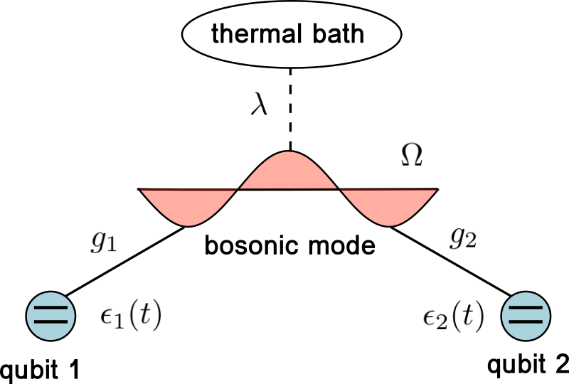
Figure 1: Schematic representation of the system under study. The qubit $i\in\{1,2\}$ is periodically driven through $\epsilon_{i}(t)$ and coupled with strength $g_{i}$ to a mode of frequency $\Omega$ of a resonator. The resonator is weakly coupled to a thermal bath with strength $\lambda$ via the bosonic operator $a+a^{\dagger}$.

The Hamiltonian of the qubit $i\in\{1,2\}$, including the coupling term to the resonator is given by

$$H_{i}(t)=\frac{\epsilon_{i}(t)}{2}\sigma_{z}^{(i)}+g_{i}(a+a^{\dagger})\sigma_{x}^{(i)},$$ (1)

where $\sigma_{j}^{(i)}$ are the Pauli matrices acting on the qubit $i$, and $a^{\dagger}$ ($a$) is the creation (destruction) operator of the bosonic mode of the resonator. The qubit $i$’s transition frequency or detuning is $\epsilon_{i}$ , which can be controlled externally as a function of time. The coupling of the qubit $i$ to the resonator is of strength $g_{i}$ and we suppose that the associated operator is transversal to the qubit $i$’s detuning operator (under this assumption, one can always rotate the qubit basis such that the coupling to the resonator is through $\sigma_{x}^{(i)}$). A possible qubit $i$ energy gap induced by a term in Eq.(1) transversal to $\sigma_{z}^{(i)}$ was neglected under the assumption that it is much smaller than the corresponding $g_{i}$’s - which is rather justified for several superconducting qubit systems Oliver et al. (2005). The full Hamiltonian for the cQED architecture is given by

$$H(t)=H_{\text{s}}(t)+H_{\text{b}}+H_{\text{sb}},$$ (2)

$$H_{\text{s}}(t)=\Omega a^{\dagger}a+\sum_{i=1}^{2}H_{i}(t),$$ (3)

where $\Omega$ is the resonator mode frequency. The term $H_{\text{b}}$ in Eq.(2) represents the bath Hamiltonian, modelled as a continuum of harmonic oscillators in thermal equilibrium at temperature $T_{\text{b}}$, with ohmic spectral density $\mathcal{J}(\omega)=\kappa\omega$, where $\kappa$ is a constant. The term $H_{\text{sb}}$ stands for the interaction between the system and the thermal bath, which in this work we suppose is through the operator $(a+a^{\dagger})$ and of strength $\lambda$. The explicit forms of $H_{\text{b}}$ and $H_{\text{sb}}$ are given in Appendix A.

The driving required for the Bell state generation protocol depends on the relative sign of the couplings $g_{i}$. We suppose that the couplings are similar in magnitude but their relative sign could be either equal or opposite, corresponding to couplings to even or odd modes of the resonator, respectively. In the following without loss of generality we will consider couplings with the same sign and the drivings in detuning chosen as

$$\epsilon(t)\equiv\epsilon_{1}(t)=\epsilon_{2}(t)=A\cos(\omega t),$$ (4)

with $A$ the amplitude and $\omega$ the frequency of the driving. For the case of opposite coupling signs, the driving should be chosen to be $\epsilon_{1}(t)=-\epsilon_{2}(t)$. It can be shown that both cases are related by a local unitary transformation $H\rightarrow\sigma_{y}^{(2)}H\sigma_{y}^{(2)}$ which keeps the entanglement generation dynamics invariant.

As we will discuss in detail in Sec.IV, to stimulate the LZS resonances necessary for this Bell state generation protocol we require that $0<|\delta_{g}|\ll g_{1}g_{2}/\Omega$, with $\delta_{g}\equiv g_{1}-g_{2}$. As the relevant involved transitions occur in a timescale $\delta_{g}^{-1}$, the smaller $\delta_{g}$, the longer it will take to reach the stationary Bell state.

To solve numerically the dynamics in the purely unitary case (considering only $H_{\text{s}}(t)$ in Eq.(2)), we diagonalize the evolution operator over a period of the driving using a 4${}^{\text{th}}$ order Trotter-Suzuki expansion. In this way we obtain the Floquet states and the associated quasienergies Shirley (1965). To study the open dynamics we evolved the system’s density operator using the Floquet-Born-Markov (FBM) master equation Kohler et al. (1998); Blattmann et al. (2015); Ferrón et al. (2016) within a moderate Rotating Wave Approximation (RWA), as is detailed in Appendix B. For the numerical simulations we truncate the Hilbert space to a finite number of photon levels. We found that retaining the first $5$ photon levels was sufficient to attain convergence.

III Unitary dynamics

In this section we focus on the unitary dynamics described by the Hamiltonian $H_{\text{s}}(t)$ defined in Eq.(3). It will be useful to define the set of Bell states of the two qubit system: $\ket{\Phi_{\pm}}\equiv\frac{1}{\sqrt{2}}(\ket{\uparrow\uparrow}\pm\ket{\downarrow\downarrow})$ and $\ket{\Psi_{\pm}}\equiv\frac{1}{\sqrt{2}}(\ket{\uparrow\downarrow}\pm\ket{\downarrow\uparrow})$, where $\sigma_{z}\ket{\uparrow}=\ket{\uparrow}$, and $\sigma_{z}\ket{\downarrow}=-\ket{\downarrow}$. The Bell states are maximally entangled and form a basis for the two qubit Hilbert space.

Figure 2(a) shows the energy spectrum of $H_{\text{s}}$ parametrized as a function of $\epsilon$, the driving variable. It can be shown that the avoided crossings at $\epsilon=\pm\Omega$ have energy gaps of first order in $g_{i}$ while for all other integer and half integer values of $\epsilon/\Omega$ the avoided crossing gaps are of second or higher order in $g_{i}$. Away from all avoided crossings, the energies and eigenstates of the system satisfy

$$H_{\text{s}}(\epsilon)\ket{N\uparrow\uparrow}\ \approx\ (N\Omega+\epsilon)\ket{N\uparrow\uparrow}$$ (5)

$$H_{\text{s}}(\epsilon)\ket{N\Psi_{\pm}}\ \approx\ \ \ \ \ \ \ \ N\Omega\ket{N\Psi_{\pm}}$$ (6)

$$H_{\text{s}}(\epsilon)\ket{N\downarrow\downarrow}\ \approx\ (N\Omega-\epsilon)\ket{N\downarrow\downarrow},$$ (7)

with $\ket{N}$ the state of the resonator with $N$ photons. In addition, it can be readily seen from Eq.(3) that for $g_{1}=g_{2}$ ($\delta_{g}=0$), the singlet states $\ket{N\Psi_{-}}$ are exact eigenstates of $H_{\text{s}}(\epsilon)$ with energy $N\Omega$. Since they are also eigenstates of the driving operator ($\propto(\sigma_{z}^{(1)}+\sigma_{z}^{(2)})$), transitions involving the states $\ket{N\Psi_{-}}$ are forbidden for $\delta_{g}=0$. In fact, defining $g\equiv(g_{1}+g_{2})/2$ we can write

$$\sum_{i}g_{i}\sigma_{x}^{(i)}=g(\sigma_{x}^{(1)}+\sigma_{x}^{(2)})+\frac{\delta_{g}}{2}(\sigma_{x}^{(1)}-\sigma_{x}^{(2)}),$$ (8)

and consider the second term in the last equation as a perturbation that induces transitions between $\ket{N\Psi_{-}}$ and $\ket{(N\pm 1)\Phi_{+}}$, since we suppose that $\delta_{g}\ll g$. This can be seen from the fact that

$$\frac{\delta_{g}}{2}(\sigma_{x}^{(1)}-\sigma_{x}^{(2)})=\delta_{g}\Big{(}\ket{\Psi_{-}}\bra{\Phi_{+}}+\ket{\Phi_{+}}\bra{\Psi_{-}}\Big{)},$$ (9)

and that the $(a+a^{\dagger})$ operator either adds or removes a photon from the resonator state which it acts on.

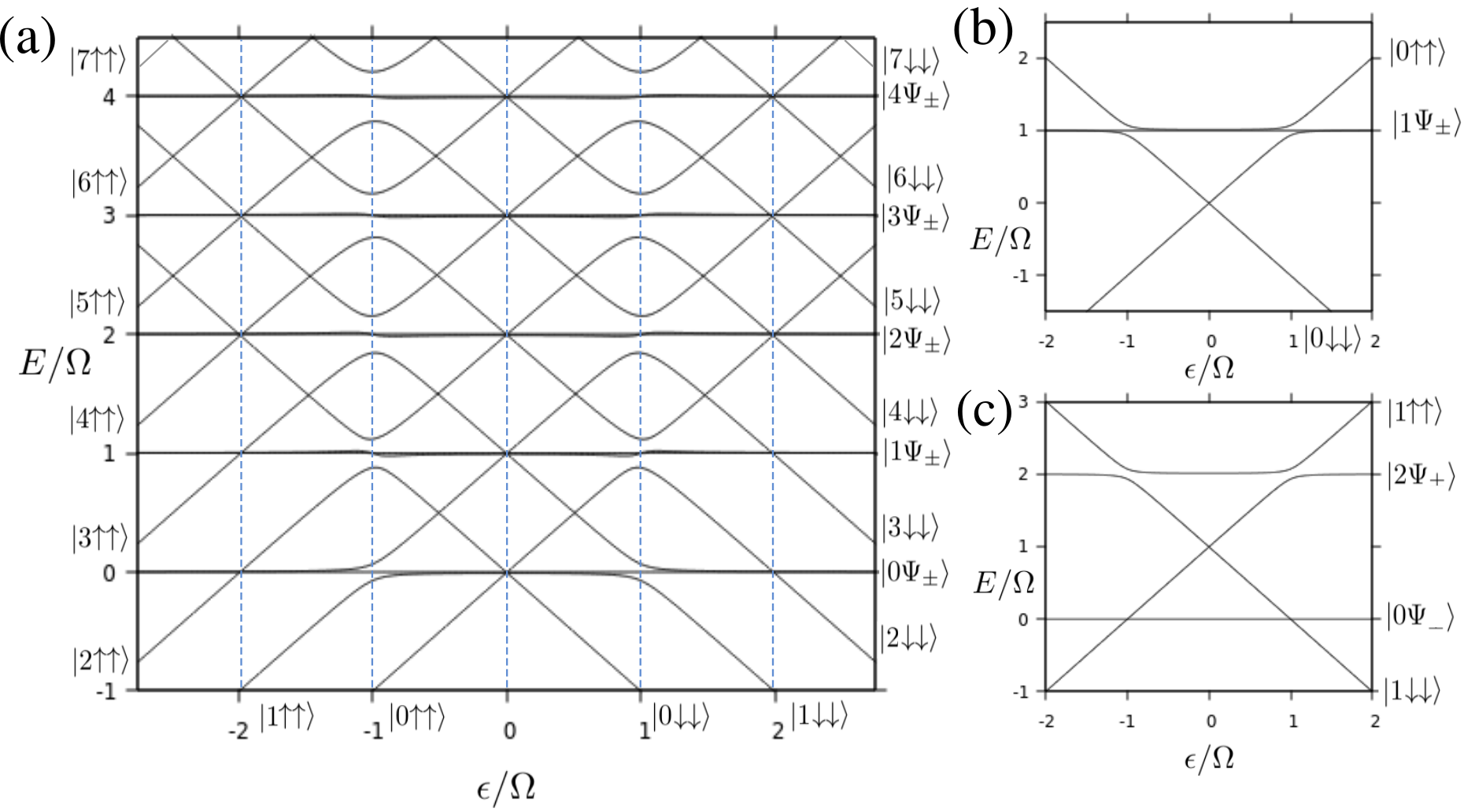
Figure 2: (a) Energy spectrum of $H_{\text{s}}$ (Eq.(3)) parametrized a function of $\epsilon/\Omega$, for $g_{1}=0.05\Omega$ and $g_{2}=0.0485\Omega$. Avoided crossings are located at integer and half-integer values of $\epsilon/\Omega$. Those at $\epsilon=\pm\Omega$ are of first order in $g_{i}$ while all others are of second and higher order in $g_{i}$. Integer values of $\epsilon/\Omega$ are marked with dotted lines. See text for more details. Energy spectra of the effective Hamiltonians (Eq.(12) and Eq.(15)) derived to study the transition (b) $\ket{0\uparrow\uparrow}\rightarrow\ket{1\Psi_{-}}$ and the transition (c) $\ket{0\Psi_{-}}\rightarrow$(other states), respectively. In all cases the asymptotic eigenstates away from avoided crossings are shown.

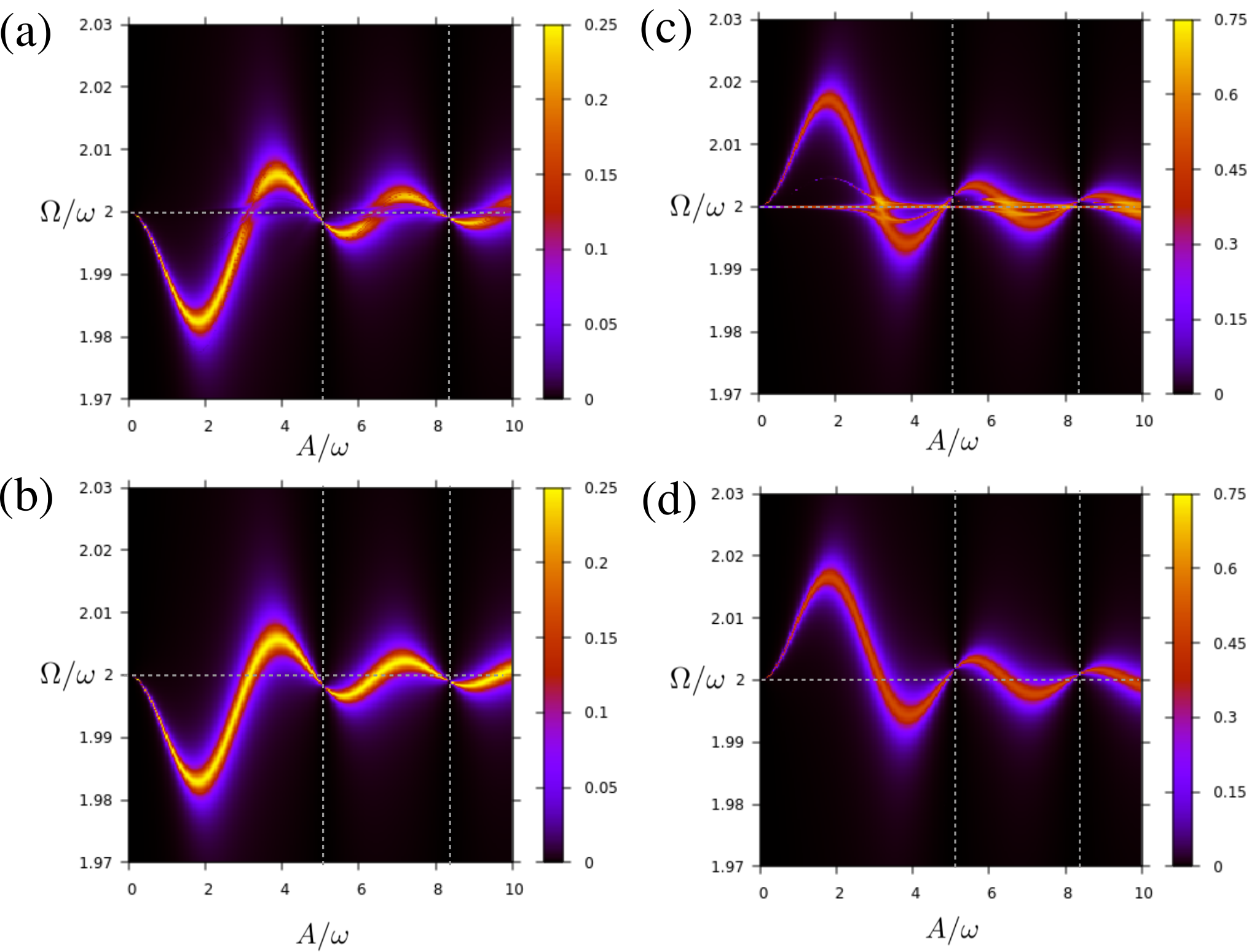
Figure 3: Upper panel: Unitary time-averaged transition probabilities calculated numerically with the Hamiltonian Eq.(3) for the transitions (a) $\ket{0\uparrow\uparrow}\rightarrow\ket{1\Psi_{-}}$ and (c) $\ket{0\Psi_{-}}\rightarrow$ (other states) , as a function of $A/\omega$ and $\Omega/\omega$. The patterns show resonances at $\Omega/\omega=n\in\mathbb{N}$ with width of order $\delta_{g}$ modulated by the $n^{\text{th}}$ Bessel function $J_{n}(A/\omega)$. Lower panel: Transition probabilities for (b) $\ket{0\uparrow\uparrow}\rightarrow\ket{1\Psi_{-}}$ and (d) $\ket{0\Psi_{-}}\rightarrow$ (other states) , calculated using the effective two-qubit Hamiltonians Eq.(12) and Eq.(15), respectively. The line $\Omega/\omega=2$ and the lines for which $A/\omega$ equals the first two zeros of the $2^{\text{nd}}$ Bessel function are indicated with grey dotted lines. In all cases the qubit-resonator coupling strengths used are $g_{1}=0.1\omega$ and $g_{2}=0.097\omega$.

In what follows we consider explicitly transitions involving $\ket{0\Psi_{-}}$ and $\ket{1\Psi_{-}}$ induced by the simultaneous effect of the time dependent driving $\epsilon(t)$, Eq.(4), and the coupling asymmetry parameter $\delta_{g}$. These transitions will be relevant for the Bell state generation mechanism once dissipation is included.

III.1 Transitions to $\ket{1\Psi_{-}}$

We begin by studying the transition probability of $\ket{0\uparrow\uparrow}\rightarrow\ket{1\Psi_{-}}$ induced by the periodic driving. We are interested in this transition because, as we will discuss in Sec.IV, $\ket{1\Psi_{-}}$ will decay into $\ket{0\Psi_{-}}$ after including dissipation, which is a maximally entangled state that is stable against photon loss.

Figure 3(a) shows the time averaged transition probability for $\ket{0\uparrow\uparrow}\rightarrow\ket{1\Psi_{-}}$, as a function of $A/\omega$ and $\Omega/\omega$, near a resonance centered around $\Omega/\omega=2$. Similar resonances of width proportional to $\delta_{g}$ are observed for all integer values of $\Omega/\omega$.

Numerically we find that for these resonances, and for $\ket{0\uparrow\uparrow}$ as the initial state, the most populated states are in the subspace $S_{1}$ spanned by $\{\ket{0\Phi_{\pm}},\ket{1\Psi_{\pm}}\}$. Projecting the Hamiltonian of Eq.(3) into $S_{1}$, the state of the resonator becomes uniquely determined by the state of the qubits (within $S_{1}$). Thus one can write the terms involving resonator operators in Eq.(3) in terms of qubit operators:

$$a^{\dagger}a|_{S_{1}}= \ket{1\Psi_{+}}\bra{1\Psi_{+}}+\ket{1\Psi_{-}}\bra{1\Psi_{-}}$$

$$= \frac{1}{2}(1-\sigma_{z}^{(1)}\sigma_{z}^{(2)}),$$ (10)

and

$$\frac{1}{2}(a+a^{\dagger})(\sigma_{x}^{(1)}\pm\sigma_{x}^{(2)})|_{S_{1}}= \ket{0\Phi_{\mp}}\bra{1\Psi_{\pm}}+\ket{1\Psi_{\pm}}\bra{0\Phi_{\mp}}$$

$$= \frac{1}{2}(\sigma_{x}^{(1)}\pm\sigma_{x}^{(2)}),$$ (11)

where now $\sigma^{(i)}_{j}$ are understood as $4\times 4$ matrices, and $|_{S_{1}}$ indicates projection into $S_{1}$. Replacing the above expressions into Eq.(3), one arrives at the effective time dependent Hamiltonian, valid for studying the transition $\ket{0\uparrow\uparrow}\rightarrow\ket{1\Psi_{-}}$:

$$H_{l}(t)=\sum_{i}\Big{(}\frac{\epsilon(t)}{2}\sigma_{z}^{(i)}+g_{i}\sigma_{x}^{(i)}\Big{)}-\frac{\Omega}{2}\sigma_{z}^{(1)}\sigma_{z}^{(2)}+\frac{\Omega}{2}.$$ (12)

Notice that Eq.(12) is the Hamiltonian of two driven qubits coupled longitudinally studied in Ref.Gramajo et al., 2017. In the present case $\Omega$ plays the role of the interaction strength between the qubits and $2g_{i}$ the role of the intrinsic qubit gaps. Figure 2(b) shows the energy spectrum of the effective Hamiltonian, Eq.(12), parametrized as a function of $\epsilon$.

In Fig. 3(b) the time averaged transition probability $\ket{0\uparrow\uparrow}\rightarrow\ket{1\Psi_{-}}$ computed numerically using Eq.(12) is displayed. The agreement with Fig. 3(a), obtained from the full Hamiltonian of Eq.(3), is excellent.

For $\delta_{g}^{2}\ll A\omega$ and neglecting the effect of $g$ on the energy spectrum, the LZS resonance condition for the transition between the two levels $\ket{0\uparrow\uparrow}$ and $\ket{1\Psi_{-}}$ is $\Omega/\omega=n$ for some integer $n$, where in this case $\Omega$ is playing the same role of the dc detuning in standard LZS interferometry, as it sets the average energy difference between the two involved levels. Thus, considering only these two levels which are separated by a gap of the order of $\delta_{g}$, resonance patterns centered around $\Omega/\omega=n$ and of width $\propto\delta_{g}J_{n}(A/\omega)$ (with $J_{n}$ the $n^{\text{th}}$ Bessel function) are expected Ashhab et al. (2007) and indeed observed in Fig. 3(b). However, the curvature of the resonances is an effect that we found numerically to be of order $g_{1}g_{2}/\Omega$, as shown in Fig. 4(a). This effect is not captured under the assumption of neglecting $g$.

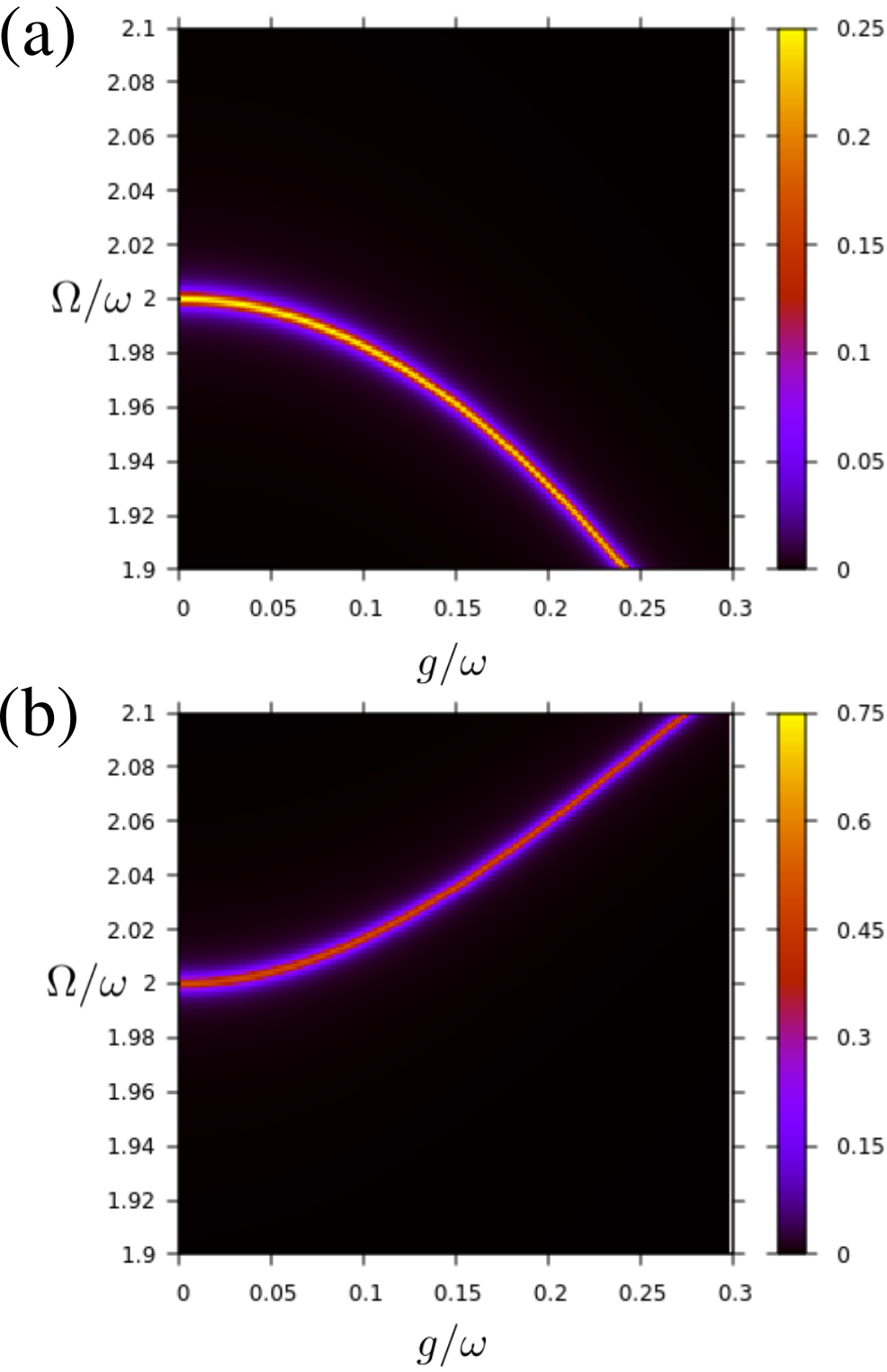
Figure 4: Unitary time averaged transition probabilities for the transitions (a) $\ket{0\uparrow\uparrow}\rightarrow\ket{1\Psi_{-}}$ and (b) $\ket{0\Psi_{-}}\rightarrow$(other states) calculated using the effective Hamiltonians Eq.(12) and Eq.(15) respectively, as a function of $g/\omega$ and $\Omega/\omega$, for $\delta_{g}=0.003\omega$ and $A=\Omega$. For small $g$, an approximately quadratic dependence of the resonance displacement as a function of $g$ is observed, with opposite curvature for both transitions.

III.2 Transitions out of $\ket{0\Psi_{-}}$

We now shift our attention to the time averaged probabilities for the $\ket{0\Psi_{-}}\rightarrow\text{(other states)}$ transition, which is defined as the sum of all transition probabilities from the initial state $\ket{0\Psi_{-}}$ to any other states different from it. We are interested in this transition because it is an indicator of the stability of $\ket{0\Psi_{-}}$ against unitary transitions induced by the driving that might take the system out of this state. Figure 3(c) shows numerical results for the corresponding transition probabilities using the full Hamiltonian Eq.(3). We have found that the only significantly populated states are in the subspace $S_{2}$ spanned by $\{\ket{0\Psi_{\pm}},\ket{1\Phi_{\pm}},\ket{2\Psi_{+}}\}$. Thus in the present case, and unlike the analysis of Sec.III.1, $5$ linearly independent states are in principle involved in the transition under study.

Numerically we found that the best two-qubit effective model is obtained when neglecting the state $\ket{2\Psi_{+}}$ in the calculation of the operator $(a+a^{\dagger})|_{S_{2}}$, and the state $\ket{0\Psi_{+}}$ in the calculation of the operator $a^{\dagger}a|_{S_{2}}$. Doing this approximation, one obtains

$$a^{\dagger}a|_{S_{2}}\approx \ket{1\Phi_{+}}\bra{1\Phi_{+}}+\ket{1\Phi_{-}}\bra{1\Phi_{-}}+2\ket{2\Psi_{+}}\bra{2\Psi_{+}}$$

$$= 1+\frac{1}{2}(\sigma_{x}^{(1)}\sigma_{x}^{(2)}+\sigma_{y}^{(1)}\sigma_{y}^{(2)}),$$ (13)

$$\frac{1}{2}(a+a^{\dagger})(\sigma_{x}^{(1)}\pm\sigma_{x}^{(2)})|_{S_{2}}\approx \ket{0\Psi_{\pm}}\bra{1\Phi_{\mp}}+\ket{1\Phi_{\mp}}\bra{0\Psi_{\pm}}$$

$$= \frac{1}{2}(\sigma_{x}^{(1)}\pm\sigma_{x}^{(2)}),$$ (14)

and we arrive at the effective Hamiltonian, valid for studying the transition $\ket{0\Psi_{-}}\rightarrow$(other states):

$$H_{\text{tr}}(t)= \sum_{i}\Big{(}\frac{\epsilon(t)}{2}\sigma_{z}^{(i)}+g_{i}\sigma_{x}^{(i)}\Big{)}+$$

$$\frac{\Omega}{2}(\sigma_{x}^{(1)}\sigma_{x}^{(2)}+\sigma_{y}^{(1)}\sigma_{y}^{(2)})+\Omega,$$ (15)

which is the Hamiltonian of two transversally coupled and symmetrically driven qubits, with $\Omega$ playing the role of the interaction strength and $2g_{i}$ the role of the intrinsic qubit gaps Gramajo et al. (2017). Figure 2(c) shows its energy spectrum parametrized as a function of $\epsilon$. Numerical results for the transition probability $\ket{0\Psi_{-}}\rightarrow\text{(other states)}$ computed from Eq.(15) are shown in Fig.3(d). Except for the additional flatter resonances around integer $\Omega/\omega$, which correspond to resonances to states outside $S_{2}$, the agreement with Fig.3(c), obtained using the full Hamiltonian Eq.(3) is remarkable.

The LZS resonance condition for both transitions, $\ket{0\Psi_{-}}\rightarrow\ket{1\uparrow\uparrow}$ and $\ket{0\Psi_{-}}\rightarrow\ket{1\downarrow\downarrow}$ respectively, is again $\Omega/\omega=n$ for some integer $n$. Resonances around these values of $\Omega/\omega$ of width $\propto\delta_{g}J_{n}(A/\omega)$ are expected and observed in Fig. 3(d), in analogy to the results of Sec.III.1. The effect of $g$ on the curvature of the resonances out of $\ket{0\Psi_{-}}$ is again of order $g_{1}g_{2}/\Omega$ but of opposite sign to that of the transitions to $\ket{1\Psi_{-}}$, as can be seen in Fig. 4(b). This implies that there are values of the driving parameters, $A$ and $\omega$, for which the transitions to $\ket{1\Psi_{-}}$ are stimulated but those out of $\ket{0\Psi_{-}}$ are not. This is the key point that will be made use of to generate Bell states once dissipation is included, as is explained below.

IV Dissipation induced Bell state generation

In the previous section we concluded that starting from the initial state $\ket{0\uparrow\uparrow}$, there are regions in the $A/\omega-\Omega/\omega$ plane where a unitary resonance to $\ket{1\Psi_{-}}$ is stimulated but no unitary resonance involving $\ket{0\Psi_{-}}$ is so. When the driving amplitude A and frequency $\omega$ are chosen as to select one of these points, the process

$$\ket{0\uparrow\uparrow}\stackrel{{\scriptstyle H_{\text{s}}(t)}}{{\rightarrow}}\ket{1\Psi_{-}}\stackrel{{\scriptstyle\text{PL}}}{{\rightarrow}}\ket{0\Psi_{-}}$$ (16)

can occur once dissipation is included, where the first transition is unitary and induced by the driven Hamiltonian $H_{s}(t)$, and the second one is the loss of a photon to the environment. The same process can also take place when starting from $\ket{0\downarrow\downarrow}$ or $\ket{0\Psi_{+}}$, since they show similar unitary resonances for $\ket{0\downarrow\downarrow}\rightarrow\ket{1\Psi_{-}}$ and $\ket{0\Psi_{+}}\rightarrow\ket{1\Psi_{-}}$.

Since the open system dynamics is linear due to the assumed weak coupling to the environment, one can understand the evolution of the system’s density matrix as the independent evolution of its ensemble members which, for $T_{\text{b}}\ll\Omega$, will eventually reach one of the states with zero photons. If the reached states are different from $\ket{0\Psi_{-}}$, they will go through the process defined in Eq.(16) ending up at least partially in $\ket{0\Psi_{-}}$. As all transitions involving $\ket{0\Psi_{-}}$ are out of resonance, gradually the population of the system’s density matrix accumulates in this state.

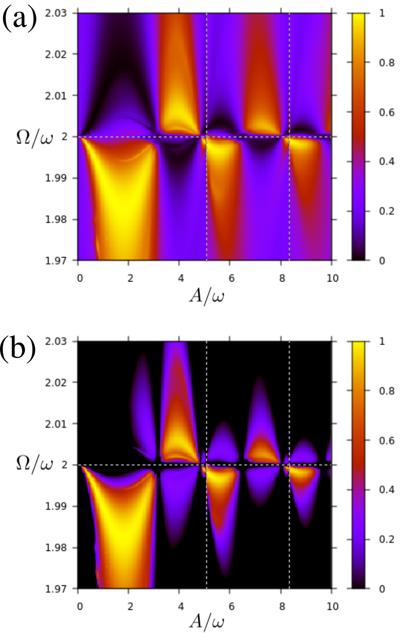
Figure 5: Time averaged (a) population of $\ket{0\Psi_{-}}$ and (b) concurrence of the steady state of the driven dissipative system of two qubits coupled to a resonator, obtained after solving numerically the FBM master equation associated to the Hamiltonian defined in Eq.(2). Asymmetrical resonance patterns are observed at integer values of $\Omega/\omega$. The coupling strengths are the same as in Fig. 3, with bath parameters $\kappa\lambda^{2}=0.0001$ and $T_{\text{b}}=0.001\omega$. The line $\Omega/\omega=2$ and the lines for which $A/\omega$ equals the first two zeros of the $2^{\text{nd}}$ Bessel function are indicated with grey dotted lines.

Figure 5(a) shows numerical results for the time averaged population of $\ket{0\Psi_{-}}$ in the stationary state as a function of $A/\omega$ and $\Omega/\omega$ obtained after solving numerically the FBM master equation for the system’s density matrix $\rho$ (see Appendix B for details). The stationary state is found to be unique and $T$-periodic in time. The behavior of the stationary population closely follows what is predicted by the previous argument: population maxima very close to $1$ are observed for points in the parameter space along the unitary resonance patterns of $\ket{0\uparrow\uparrow}\rightarrow\ket{1\Psi_{-}}$ and population minima, very close to $0$, are obtained for points along the unitary $\ket{0\Psi_{-}}\rightarrow\text{(other states)}$ resonances.

To quantify the degree of entanglement of the qubits, we use the concurrence as a measure Wootters (1998),

$$\mathcal{C}[\rho_{\text{q}}]=\max\{0,r_{3}-r_{2}-r_{1}-r_{0}\},$$ (17)

defined in terms of the qubits’ density matrix $\rho_{\text{q}}=\text{Tr}_{\text{r}}(\rho)$, where the trace operation is over the states of the resonator and $r_{i}$ are the real-valued eigenvalues of

$$\sqrt{\sqrt{\rho_{\text{q}}}\sigma_{y}^{(1)}\sigma_{y}^{(2)}\rho_{\text{q}}^{*}\sigma_{y}^{(1)}\sigma_{y}^{(2)}\sqrt{\rho_{\text{q}}}},$$ (18)

sorted in ascending order, where $\rho_{\text{q}}^{*}$ is the complex conjugate of $\rho_{\text{q}}$ and the conjugation must be done in a separable basis. The concurrence takes a value of $0$ for a separable state, a value of $1$ for a maximally entangled state, and values in between for partially entangled states.

Figure 5(b) shows the time averaged concurrence of the stationary state. It is observed that the maxima of the concurrence that are close to $1$ are achieved only when the state $\ket{0\Psi_{-}}$ is populated, indicating that this is the only maximally entangled state that is generated. It is also noteworthy that for driving parameters lying outside the mentioned resonances, which constitute the vast majority of the points in the $A/\omega-\Omega/\omega$ plane (including the case of no driving at all $A=0$), the stationary state is either separable or almost separable.

As we have already mentioned, to attain $\ket{0\Psi_{-}}\bra{0\Psi_{-}}$ as the stationary state of the system, a necessary condition is to find points in the plane $A/\omega-\Omega/\omega$ where the resonance conditions for the transitions to $\ket{1\Psi_{-}}$ and out of $\ket{0\Psi_{-}}$ do not overlap. This can only be fulfilled if the maximum resonance deviation from the condition $\Omega/\omega=n$ (of order $g_{1}g_{2}/\Omega$) is much greater than the resonance width (of order $\delta_{g}$), and this the source of the requirement $\delta_{g}\ll g_{1}g_{2}/\Omega$ . The optimal entanglement generation (maximal area and intensity of concurrence patterns) is achieved for amplitudes $A=\Omega$ and frequencies $\omega$ such that $\Omega$ is below an integer multiple of $\omega$ by a frequency of the order of $g_{1}g_{2}/\Omega$, i.e. $A=\Omega=n\omega-\mathcal{O}(g_{1}g_{2}/\Omega)$.

Finally, Fig.6 shows the temporal dynamics of relevant populations of the system’s density matrix at a point of high entanglement generation $A=\Omega=1.983\omega$, for the system starting in the state $\rho_{0}=\ket{0\uparrow\uparrow}\bra{0\uparrow\uparrow}$. It is seen that even though the dynamics of the populations is complicated, a clear resonance to the state $\ket{1\Psi_{-}}$ is stimulated in a timescale of the order of $\delta_{g}^{-1}$, which gradually decays into $\ket{0\Psi_{-}}$ via photon loss to the environment. Population accumulates in this state, and given enough time the system ends up essentially at $\rho_{\infty}=\ket{0\Psi_{-}}\bra{0\Psi_{-}}$.

We thus conclude that by applying a driving with appropriate amplitude and frequency it is possible to populate the maximally entangled state $\ket{0\Psi_{-}}$ independently of the initial state of the system.

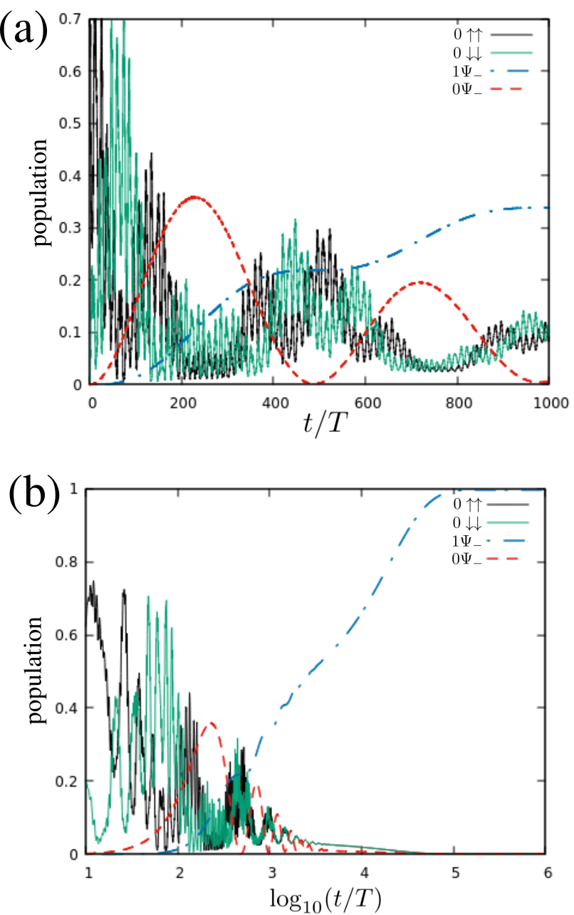
Figure 6: Temporal dependence of the system’s density matrix populations, starting from the initial state $\ket{0\uparrow\uparrow}\bra{0\uparrow\uparrow}$, for up to (a) $1000$ (linear scale) and (b) $10^{6}$ (log scale) driving periods, dissipation included. The driving parameters are $A=\Omega=1.983\omega$, and the rest of the parameters are the same as in Fig.5. The populations of $\ket{0\uparrow\uparrow}$, $\ket{0\downarrow\downarrow}$, $\ket{0\Psi_{-}}$ and $\ket{1\Psi_{-}}$ are shown. It is seen that for short times a resonance between $\ket{0\uparrow\uparrow}$, $\ket{0\downarrow\downarrow}$ and $\ket{1\Psi_{-}}$ is stimulated. For later times and via photon loss population gradually accumulates in $\ket{0\Psi_{-}}$.

V Conclusions

In this work we have presented an entanglement generation protocol for a system of two qubits coupled through a resonator. A maximally entangled steady state is achieved when a symmetric ac driving is applied over both qubits with appropriate amplitude and frequency.

The areas of entanglement generation in the $A/\omega$-$\Omega/\omega$ plane are associated to resonant unitary transitions into $\ket{1\Psi_{-}}$ and out of $\ket{0\Psi_{-}}$. If the driving is such that transitions to $\ket{1\Psi_{-}}$ are in resonance, but transitions out of $\ket{0\Psi_{-}}$ are not, once dissipation is included the system will accumulate population in $\ket{0\Psi_{-}}$ via photon loss from $\ket{1\Psi_{-}}$. All the relevant features of the unitary resonance patterns were described in terms of effective Hamiltonians for two driven qubits.

The optimal steady state entanglement generation (in terms of maximal area and intensity) is attained for driving amplitudes $A=\Omega$ and frequencies such that $\Omega/\omega$ is slightly below an integer number.

The proposed protocol shows advantages with respect to other methods for entanglement generation. Due to dissipation, the steady state is independent of the initial state of the system Kraus et al. (2008); Verstraete et al. (2009) and, once the entangled state is obtained, it is protected from environmental effects for as long as the driving is applied. Moreover, the present proposal allows entangling distant and strongly driven qubits which are, for example, a microwave waveguide apart. Therefore, it is expected that our scheme could add a robust means to realize entanglement protocols in setups extensively used nowadays in cQED Blais et al. (2020, 2021).

Acknowlegments

We acknowledge support from CNEA, CONICET (PIP11220150100756), ANPCyT (PICT2016-0791 and PICT2019-0654) and UNCuyo (06/C591).

Appendix A Model of the environment

We model the bath and its interaction with the system using the Caldeira-Leggett model Breuer and Petruccione (2006):

$$H_{\text{b}}= \int_{0}^{\infty}d\omega\omega b_{\omega}^{\dagger}b_{\omega}$$ (19)

$$H_{\text{sb}}= \lambda A\int_{0}^{\infty}d\omega\sqrt{\mathcal{J}(\omega)}(b_{\omega}+b_{\omega}^{\dagger})+H_{\text{rn}}$$ (20)

$$H_{\text{rn}}= \lambda^{2}A^{2}\int_{0}^{\infty}d\omega\frac{\mathcal{J}(\omega)}{\omega},$$ (21)

where $b_{\omega}$ and $b_{\omega}^{\dagger}$ are the creation and destruction operators of the harmonic oscillator continuum, $A$ is a unitless system operator, $\lambda$ is a coupling strength, and $H_{\text{rn}}$ is a renormalization term to cancel all Lamb shifts induced on the system by the thermal bath.

For the system under study we chose $A=a+a^{\dagger}$ and $\mathcal{J}(\omega)=\kappa\omega$, with $\kappa$ a constant with units of energy^-2. Usually, it is necessary to put a cutoff frequency in the bath spectral density, but for our purposes, and since we have already cancelled out the Lamb shifts, it is permissible to take this cutoff frequency as infinity (greater than all energy scales of the problem) as we have implicitly done by the choice of $\mathcal{J}(\omega)$.

Appendix B Floquet-Born-Markov master equation

Floquet theory is widely used to study time periodic unitary quantum systems Shirley (1965). It shows that for a quantum system with a $T$-periodic Hamiltonian $H(t)$, all solutions are a linear combination of a single basis of states of the form $e^{-i\epsilon_{\alpha}t}\ket{u_{\alpha}(t)}$. Here, $\ket{u_{\alpha}(t)}$ is $T$-periodic and is called a Floquet state, and $\epsilon_{\alpha}$ is called its corresponding quasienergy. To find the Floquet states and their quasienergies it is customary to diagonalize the evolution operator $U(t,t_{0})$ over a period of the driving, since the Floquet states satisfy the eigenvalue equation:

$$U(t+T,t)\ket{u_{\alpha}(t)}=e^{-i\epsilon_{\alpha}T}\ket{u_{\alpha}(t)}.$$ (22)

The Floquet-Born-Markov master equation Kohler et al. (1998); Ferrón et al. (2012); Blattmann et al. (2015) allows modelling dissipative processes in periodically driven systems for sufficiently weak coupling to the environment. It is a linear Markovian differential equation for the time evolution of the system’s density matrix:

$$\partial_{t}\rho_{\alpha\beta}(t)=-i(\epsilon_{\alpha}-\epsilon_{\beta})\rho_{\alpha\beta}(t)+\sum_{\alpha^{\prime}\beta^{\prime}}L_{\alpha\beta\alpha^{\prime}\beta^{\prime}}(t)\rho_{\alpha^{\prime}\beta^{\prime}}(t),$$ (23)

where $\rho_{\alpha\beta}(t)=\bra{u_{\alpha}(t)}\rho(t)\ket{u_{\beta}(t)}$ are the components of the system’s density matrix in a Floquet basis. The first term in (23) corresponds to the unitary evolution of the system, while the second one takes into account dissipative effects. The transition rates $L_{\alpha\beta\alpha^{\prime}\beta^{\prime}}(t)$ are $T$-periodic and can be Fourier expanded as

$$L_{\alpha\beta\alpha^{\prime}\beta^{\prime}}(t)=\sum_{q}L^{q}_{\alpha\beta\alpha^{\prime}\beta^{\prime}}e^{-iq\omega t},$$ (24)

with $q\in\mathbb{Z}$, and where the coefficients $L^{q}_{\alpha\beta\alpha^{\prime}\beta^{\prime}}$ are given by

$$L^{q}_{\alpha\beta\alpha^{\prime}\beta^{\prime}}=\lambda^{2}\sum_{k}\Big{(}g_{\alpha\alpha^{\prime}}^{k}A_{\alpha\alpha^{\prime}}^{k}A_{\beta^{\prime}\beta}^{-k-q}+g_{\beta\beta^{\prime}}^{k}A_{\alpha\alpha^{\prime}}^{k-q}A_{\beta^{\prime}\beta}^{-k}$$

$$-\sum_{\eta}(\delta_{\beta\beta^{\prime}}g_{\eta\alpha^{\prime}}^{k}A_{\alpha\eta}^{-k-q}A_{\eta\alpha^{\prime}}^{k}+\delta_{\alpha\alpha^{\prime}}g_{\eta\beta^{\prime}}^{k}A_{\beta^{\prime}\eta}^{-k}A_{\eta\beta}^{k-q})\Big{)}.$$ (25)

In the last expression, the index $\eta$ runs over the indices of the Floquet basis, $\delta_{\alpha\beta}$ is the Kronecker delta and we defined

$$A_{\alpha\beta}^{q}=\sum_{k}\bra{u_{\alpha}^{k}}A\ket{u_{\beta}^{q+k}}$$ (26)

and

$$g_{\alpha\beta}^{k}=g(\epsilon_{\alpha}-\epsilon_{\beta}+k\omega).$$ (27)

In Eq.(26), $\ket{u_{\alpha}^{k}}$ is the $k$th Fourier component of the Floquet state $\ket{u_{\alpha}(t)}$. In Eq. (27), $g(\omega^{\prime})$ is the Fourier transformed correlation function of the thermal bath, which can be expressed in terms of its spectral density and the Bose occupation number $n_{T_{\text{b}}}(\omega^{\prime})=1/(e^{\omega^{\prime}/T_{\text{b}}}-1)$ as

$$g(\omega^{\prime})=\begin{cases}\mathcal{J}(\omega^{\prime})n_{T_{\text{b}}}(\omega^{\prime})\ \ \ &\Leftarrow\omega^{\prime}>0\\ -\mathcal{J}(-\omega^{\prime})n_{T_{\text{b}}}(\omega^{\prime})&\Leftarrow\omega^{\prime}<0,\end{cases}$$ (28)

with the value of $g$ at $\omega^{\prime}=0$ obtained by taking the appropriate limit.

For sufficiently weak coupling to the environment, such that the maximum rate of relaxation or decoherence is much smaller than the driving frequency, a (moderate) RWA is justified in the transition rates, Eq.(24). This sets the terms with $q\neq 0$ effectively to zero, yielding the simplified expression:

$$L_{\alpha\beta\alpha^{\prime}\beta^{\prime}}\approx R_{\alpha\beta\alpha^{\prime}\beta\beta^{\prime}}+R_{\beta\alpha\beta^{\prime}\alpha^{\prime}}^{*}-\sum_{\eta}(\delta_{\beta\beta^{\prime}}R_{\eta\eta\alpha^{\prime}\alpha}+\delta_{\alpha\alpha^{\prime}}R_{\eta\eta\beta^{\prime}\beta}^{*}),$$ (29)

in terms of the quantities

$$R_{\alpha\beta\alpha^{\prime}\beta^{\prime}}=\sum_{k}g_{\alpha\alpha^{\prime}}^{k}A_{\alpha\alpha^{\prime}}^{k}A_{\beta\beta^{\prime}}^{-k}.$$ (30)

With this approximation, Eq.(23) no longer depends explicitly on time in the Floquet basis.

For the cases studied in this work, it was found that the operator $\Lambda_{\alpha\beta\alpha^{\prime}\beta^{\prime}}=-i(\epsilon_{\alpha}-\epsilon_{\beta})\delta_{\alpha\alpha^{\prime}}\delta_{\beta\beta^{\prime}}+L_{\alpha\beta\alpha^{\prime}\beta^{\prime}}$ can be numerically diagonalized in terms of left and right eigenvectors which are density matrices. That is,

$$\Lambda\rho_{\mu}^{\text{R}}=\rho_{\mu}^{\text{L}}\Lambda=\zeta_{\mu}\rho_{\mu},$$ (31)

with $\zeta_{\mu}\in\mathbb{C}$ and $\frac{1}{N}\text{Tr}(\rho_{\mu}^{\text{L}}\rho_{\nu}^{\text{R}})=\delta_{\mu\nu}$, where $N$ is the dimension of the system’s Hilbert space. Once these eigenvectors and eigenvalues are obtained, density matrices can be evolved readily by projecting on this eigensystem,

$$\rho(t)=\sum_{\mu}c_{\mu}e^{\zeta_{\mu}(t-t_{0})}\rho_{\mu}^{\text{R}},\ \ c_{\mu}=\frac{1}{N}\text{Tr}(\rho_{\mu}^{\text{L}}\rho(t_{0})).$$ (32)

The real parts of $\zeta_{\mu}$ (which are always negative) are the decoherence and relaxation rates. The stationary state $\rho_{\infty}$, which for all cases studied in this work can be found and is unique, is defined (in the Floquet basis) as the state $\rho^{\text{R}}_{\mu}$ with $\zeta_{\mu}=0$. It is constant in the Floquet basis and therefore $T$-periodic in the original system basis.

To calculate time averaged functions $f(\rho)$ of the system’s density matrix in the stationary state, such as populations or concurrence, we make use of the periodicity of $\rho_{\infty}$ and numerically integrate

$$\bar{f}=\frac{1}{T}\int_{0}^{T}dtf(\rho_{\infty}(t)).$$ (33)

References

- Kraus et al. (2008) B. Kraus, H. P. Büchler, S. Diehl, A. Kantian, A. Micheli, and P. Zoller, Phys. Rev. A 78, 042307 (2008).
- Verstraete et al. (2009) F. Verstraete, M. M. Wolf, and J. Ignacio Cirac, 5, 633 EP (2009).
- Tacchino et al. (2018) F. Tacchino, A. Auffèves, M. F. Santos, and D. Gerace, Phys. Rev. Lett. 120, 063604 (2018).
- Král et al. (2007) P. Král, I. Thanopulos, and M. Shapiro, Rev. Mod. Phys. 79, 53 (2007).
- Maeda et al. (2006) H. Maeda, J. H. Gurian, D. V. L. Norum, and T. F. Gallagher, Phys. Rev. Lett. 96, 073002 (2006).
- Zhou et al. (2017) B. B. Zhou, A. Baksic, H. Ribeiro, C. Yale, F. Heremans, P. Jerger, A. Auer, G. Burkard, A. Clerk, and D. Awschalom, Nature Physics 13, 330 (2017).
- Shankar et al. (2013) S. Shankar, M. Hatridge, Z. Leghtas, K. Sliwa, A. Narla, U. Vool, S. M. Girvin, L. Frunzio, M. Mirrahimi, and M. H. Devoret, Nature 504, 419 (2013).
- Leghtas et al. (2013) Z. Leghtas, U. Vool, S. Shankar, M. Hatridge, S. M. Girvin, M. H. Devoret, and M. Mirrahimi, Physical Review A 88, 023849 (2013).
- Kimchi-Schwartz et al. (2016) M. E. Kimchi-Schwartz, L. Martin, E. Flurin, C. Aron, M. Kulkarni, H. E. Tureci, and I. Siddiqi, Phys. Rev. Lett. 116, 240503 (2016).
- Quintana et al. (2013) C. M. Quintana, K. D. Petersson, L. W. McFaul, S. J. Srinivasan, A. A. Houck, and J. R. Petta, Phys. Rev. Lett. 110, 173603 (2013).
- Campagne-Ibarcq et al. (2018a) P. Campagne-Ibarcq, E. Zalys-Geller, A. Narla, S. Shankar, P. Reinhold, L. Burkhart, C. Axline, W. Pfaff, L. Frunzio, R. J. Schoelkopf, and M. H. Devoret, Phys. Rev. Lett. 120, 200501 (2018a).
- Li et al. (2020) R. Li, D. Yu, S.-L. Su, and J. Qian, Phys. Rev. A 101, 042328 (2020).
- Krauter et al. (2011) H. Krauter, C. A. Muschik, K. Jensen, W. Wasilewski, J. M. Petersen, J. I. Cirac, and E. S. Polzik, Phys. Rev. Lett. 107, 080503 (2011).
- Barreiro et al. (2011) J. T. Barreiro, M. Müller, P. Schindler, D. Nigg, T. Monz, M. Chwalla, M. Hennrich, C. F. Roos, P. Zoller, and R. Blatt, Nature 470, 486 EP (2011).
- Lin et al. (2013) Y. Lin, J. P. Gaebler, F. Reiter, T. R. Tan, R. Bowler, A. S. Sørensen, D. Leibfried, and D. J. Wineland, 504, 415 EP (2013).
- Kienzler et al. (2015) D. Kienzler, H.-Y. Lo, B. Keitch, L. de Clercq, F. Leupold, F. Lindenfelser, M. Marinelli, V. Negnevitsky, and J. P. Home, Science 347, 53 (2015).
- DiCarlo et al. (2010) L. DiCarlo, M. D. Reed, L. Sun, B. R. Johnson, J. M. Chow, J. M. Gambetta, L. Frunzio, S. M. Girvin, M. H. Devoret, and R. J. Schoelkopf, Nature 467, 574 (2010).
- Gramajo et al. (2018) A. L. Gramajo, D. Domínguez, and M. J. Sánchez, Phys. Rev. A 98, 042337 (2018).
- Gramajo et al. (2021) A. L. Gramajo, D. Domínguez, and M. J. Sánchez, Phys. Rev. A 104, 032410 (2021).
- Blais et al. (2004) A. Blais, R.-S. Huang, A. Wallraff, S. M. Girvin, and R. J. Schoelkopf, Phys. Rev. A 69, 062320 (2004).
- Wallraff et al. (2004) A. Wallraff, D. I. Schuster, A. Blais, L. Frunzio, R.-S. Huang, J. Majer, S. Kumar, S. M. Girvin, and R. J. Schoelkopf, Nature 431, 162 (2004).
- Xiang et al. (2013) Z.-L. Xiang, S. Ashhab, J. You, and F. Nori, Reviews of Modern Physics 85, 623 (2013).
- Blais et al. (2020) A. Blais, S. M. Girvin, and W. D. Oliver, Nature Physics 16, 247 (2020).
- Blais et al. (2021) A. Blais, A. L. Grimsmo, S. M. Girvin, and A. Wallraff, Rev. Mod. Phys. 93, 025005 (2021).
- Koch et al. (2007) J. Koch, T. Yu, M. Terri, J. Gambetta, A. A. Houck, D. I. Schuster, J. Majer, A. Blais, M. Devoret, S. Girvin, and R. J. Schoelkopf, Phys. Rev. A 76, 042319 (2007).
- Gu et al. (2017) X. Gu, A. F. Kockum, A. Miranowicz, Y. xi Liu, and F. Nori, Physics Reports 718-719, 1 (2017), microwave photonics with superconducting quantum circuits.
- Bonifacio et al. (2020) M. Bonifacio, D. Domínguez, and M. J. Sánchez, Physical Review B 101, 245415 (2020).
- Fink et al. (2009) J. M. Fink, R. Bianchetti, M. Baur, M. Göppl, L. Steffen, S. Filipp, P. J. Leek, A. Blais, and A. Wallraff, Phys. Rev. Lett. 103, 083601 (2009).
- Paik et al. (2011) H. Paik, D. I. Schuster, L. S. Bishop, G. Kirchmair, G. Catelani, A. P. Sears, B. R. Johnson, M. J. Reagor, L. Frunzio, L. I. Glazman, S. M. Girvin, M. H. Devoret, and R. J. Schoelkopf, Phys. Rev. Lett. 107, 240501 (2011).
- Dewes et al. (2012) A. Dewes, R. Lauro, F. R. Ong, V. Schmitt, P. Milman, P. Bertet, D. Vion, and D. Esteve, Phys. Rev. B 85, 140503 (2012).
- DiCarlo et al. (2009) L. DiCarlo, J. M. Chow, J. M. Gambetta, L. S. Bishop, B. R. Johnson, D. Schuster, J. Majer, A. Blais, L. Frunzio, S. Girvin, et al., Nature 460, 240 (2009).
- Stern et al. (2014) M. Stern, G. Catelani, Y. Kubo, C. Grezes, A. Bienfait, D. Vion, D. Esteve, and P. Bertet, Phys. Rev. Lett. 113, 123601 (2014).
- Johnson et al. (2010) B. R. Johnson, M. D. Reed, A. A. Houck, D. I. Schuster, L. S. Bishop, E. Ginossar, J. M. Gambetta, L. DiCarlo, L. Frunzio, S. M. Girvin, and R. J. Schoelkopf, Nature Physics 6, 663 (2010).
- Walter et al. (2017) T. Walter, P. Kurpiers, S. Gasparinetti, P. Magnard, A. Potočnik, Y. Salathé, M. Pechal, M. Mondal, M. Oppliger, C. Eichler, and A. Wallraff, Phys. Rev. Applied 7, 054020 (2017).
- van Loo et al. (2013) A. F. van Loo, A. Fedorov, K. Lalumiere, B. C. Sanders, A. Blais, and A. Wallraff, Science 342, 1494–1496 (2013).
- Eichler et al. (2012) C. Eichler, C. Lang, J. M. Fink, J. Govenius, S. Filipp, and A. Wallraff, Physical Review Letters 109 (2012), 10.1103/physrevlett.109.240501.
- Didier et al. (2015) N. Didier, J. Bourassa, and A. Blais, Physical Review Letters 115 (2015), 10.1103/physrevlett.115.203601.
- Campagne-Ibarcq et al. (2018b) P. Campagne-Ibarcq, E. Zalys-Geller, A. Narla, S. Shankar, P. Reinhold, L. Burkhart, C. Axline, W. Pfaff, L. Frunzio, R. J. Schoelkopf, and M. H. Devoret, Phys. Rev. Lett. 120, 200501 (2018b).
- S.N. Shevchenko (2010) F. N. S.N. Shevchenko, S. Ashhab, Physics Reports 492, 1 (2010).
- Oliver and Valenzuela (2009) W. D. Oliver and S. O. Valenzuela, Quantum Information Processing 8, 261 (2009).
- Ferrón et al. (2012) A. Ferrón, D. Domínguez, and M. J. Sánchez, Phys. Rev. Lett. 109, 237005 (2012).
- Ferrón et al. (2016) A. Ferrón, D. Domínguez, and M. J. Sánchez, Phys. Rev. B 93, 064521 (2016).
- Gramajo et al. (2019) A. L. Gramajo, D. Domínguez, and M. J. Sánchez, Phys. Rev. B 100, 075410 (2019).
- Bronn et al. (2015) N. T. Bronn, E. Magesan, N. A. Masluk, J. M. Chow, J. M. Gambetta, and M. Steffen, IEEE Transactions on Applied Superconductivity 25, 1 (2015).
- Oliver et al. (2005) W. D. Oliver, Y. Yu, J. C. Lee, K. K. Berggren, L. S. Levitov, and T. P. Orlando, Science 310, 1653 (2005).
- Shirley (1965) J. H. Shirley, Physical Review 138, B979 (1965).
- Kohler et al. (1998) S. Kohler, R. Utermann, P. Hänggi, and T. Dittrich, Phys. Rev. E 58, 7219 (1998).
- Blattmann et al. (2015) R. Blattmann, P. Hänggi, and S. Kohler, Phys. Rev. A 91, 042109 (2015).
- Gramajo et al. (2017) A. L. Gramajo, D. Domínguez, and M. J. Sánchez, Eur. Phys. J. B 90, 255 (2017).
- Ashhab et al. (2007) S. Ashhab, J. R. Johansson, A. M. Zagoskin, and F. Nori, Phys. Rev. A 75, 063414 (2007).
- Wootters (1998) W. K. Wootters, Physical Review Letters 80, 2245 (1998).
- Breuer and Petruccione (2006) H.-P. Breuer and F. Petruccione, The Theory of Open Quantum Systems (Oxford University Press, 2006).