The Case for Learned In-Memory Joins

Abstract

In-memory join is an essential operator in any database engine. It has been extensively investigated in the database literature. In this paper, we study whether exploiting the CDF-based learned models to boost the join performance is practical or not. To the best of our knowledge, we are the first to fill this gap. We investigate the usage of CDF-based partitioning and learned indexes (e.g., Recursive Model Index (RMI) and RadixSpline) in the three join categories; indexed nested loop join (INLJ), sort-based joins (SJ) and hash-based joins (HJ). Our study shows that there is a room to improve the performance of INLJ and SJ categories through our proposed optimized learned variants. Our experimental analysis showed that these proposed learned variants of INLJ and SJ consistently outperform the state-of-the-art techniques.

I Introduction

In-memory join is an essential operator in any database engine. It has been extensively investigated in the database literature (e.g., [22, 20, 2, 4, 62, 8, 34, 6]). Basically, in-memory join algorithms can be categorized into three main categories: nested loop joins (e.g., [22, 20]), whether non-indexed or indexed, sort-based joins (e.g., [2, 4]), and hash-based joins (e.g., [62, 8, 34, 6]). Many recent studies (e.g., [4, 57]) have shown that the design, as well as the implementation details, have a substantial impact on the join performance, specially on the modern hardware.

Meanwhile, there has been growing interest in exploiting learned models, such as CDF-based partitioning [31, 32] and Recursive Model Indexes (RMI) [31], to enhance or replace traditional data structures and algorithms, such as indexing [31, 27, 19, 15, 50, 49], sorting [32, 33], and hashing [56, 29]. These learned data structures and algorithms can outperform their traditional counterparts on practical workloads as they are better in exploiting trends in the input data and instance-optimizing the performance. Along this line of work, the idea of using CDF-based learned models to improve the performance of in-memory join algorithms was suggested in [31]. However, this idea was neither fully investigated nor supported with an experimental evidence.

In this paper, we aim to study, in details, whether exploiting the CDF-based learned models to boost the performance of in-memory joins is a beneficial idea or not. In particular, we investigate the performance of the three join categories; indexed nested loop join (INLJ), sort-based joins (SJ) and hash-based joins (HJ), while modifying or replacing their different phases (e.g., indexing, sorting, joining) with CDF-based and RMI-based variants. Our paper has the following three main contributions:

Investigating Alternatives of Using Learned Models for Joins. Although the learned model ideas have been introduced in previous works, none of them has been studied in the context of join processing. Therefore, for each join category, we first discuss the straightforward alternatives of directly integrating learned models with its phases. For example, in INLJ, RMI can be used to replace the built index on the indexed relation. In SJ, the LearnedSort algorithm [32] can be used to replace the sorting phase. In HJ, RMI or CDF-based partitioning function can be used to replace the hash function that is used to build the hash table. While investigating the different alternatives, we come up with two interesting observations. First, it is hard to use learned models to improve over classical hash join methods [62, 34, 6]. Second, using learned models ”as-is” in replacing INLJ and SJ phases is sub-optimal. For example, using the LearnedSort algorithm [32] as a black-box replacement for the sorting algorithms used in the state-of-the-art SJ techniques, such as MPSM [2] and MWAY [62], leads to repeating unnecessary work, and hence increases the overall execution time. Another example is replacing the hash functions used in hash-based INLJ with RMI models. Unfortunately, this also leads to a poor performance (i.e., high overall latency) as RMI requires a significant overhead to correct its mispredictions.

Optimized Learned Join Variants. To overcome the performance limitations of using learned models as black-boxes, we introduce optimized variants of the learned join algorithms in the INLJ and SJ join categories, which lead to several performance improvements. In particular, in INLJ category, we introduced two efficient variants of learned INLJ. The first variant, namely Gapped RMI INLJ, employs an efficient read-only RMI that is built using the concept of model-based insertion introduced in [15]. To further improve the performance of this variant, we introduced a cache-optimized hierarchical buffering technique, namely Requests Buffer, to temporarily store the probe (i.e., lookup) operations over the RMI, which reduces the cache misses, and hence improves the join throughput. We also provided a cache complexity analysis for this buffering technique, and proved its matching to the caching analytical bounds in [20]. The second variant, namely learned-based hash INLJ, employs RadixSpline to build a hash index that is useful in some scenarios, like joining sequential datasets. In SJ category, we proposed a new sort-based join, namely L-SJ, that exploits a CDF-based model to improve the different SJ phases (e.g., sort and join) by just scaling up its prediction degree. L-SJ has the following two merits. First, it combines CDF-based partitioning with AVX sort [4] to provide a new efficient sorting phase. We also provided a complexity analysis for this new sorting phase. Second, it employs the CDF-based model to reduce the amount of redundant join checks in the merge-join phase.

Extensive Experimental Evaluation. To achieve a deeper understanding of the practicality of using learned models with joins, we conducted a detailed evaluation study for both learned and non-learned variants in the three join categories, using different real (SOSD [44]) and synthetic datasets. In particular, we compare the optimized learned join variants against, seven INLJ baselines (three off-shelf learned (RMI [31], RadixSpline [27], ALEX [15]), two tree-based (Cache-Sensitive Search Trees [22], Adaptive Radix Trie [38]), and two hash-based (bucket chaining and Cuckoo hash) indexes), two SJ baselines (MPSM [2], MWAY [4]), and two HJ baselines (non-partitioned [62], partitioned [57]). We show that, the two optimized variants of learned INLJ, using Gapped RMI, can provide better performance than almost all traditional baselines (e.g., 2.7X faster than hash-based INLJ) in many scenarios and with different datasets. In addition, the optimized learned SJ variant can be 2X faster than MWAY [4], which is the best sort-based join baseline in the literature. We also extend this analysis to duplicate datasets, multiple dataset sizes and ratios, skewness and parallelism degrees, and other performance counters (e.g., cache misses, branch misses and instructions) as well as hardware aspects (e.g., NUMA awareness and page sizes).

We believe our study is beneficial for researchers and practitioners, who are interested in building instance-optimized DBMS, like SageDB [30], as it provides good practices for implementing efficient learned join algorithms.

II Background

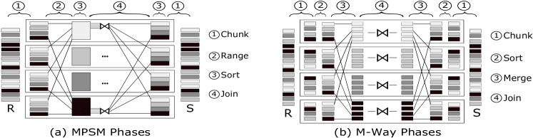
Figure 1: Sort-based Joins: MPSM and MWAY

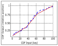
Figure 2: Linear Models Approximation of CDF

In this section, we provide a brief background on the different join categories that we study (section II-A to II-C), and the learned concepts and indexes we exploit (Section II-D).

II-A Indexed Nested Loop Joins (INLJ)

This is the most basic type of join. Here, we assume that one input relation, say $R$, has an index on the join key. Then, the algorithm simply scans each tuple in the second relation $S$, uses the index to fetch the tuples from $R$ with the same join key, and finally performs the join checks. INLJ achieves a good performance when using a clustered index as the tuples with the same join key will have a spatial locality, and hence improves the caching behavior.

II-B Sort-based Joins (SJ)

The main idea of sort-based join is to first sort both input relations on the same join key. Then, the sorted relations are joined using an efficient merge-join algorithm to find all matching tuples. Here, we describe the details of two efficient multi-core variants of sort-based joins, MPSM [2] and MWAY [4], as follows:

Massively Parallel Sort-Merge (MPSM). The idea of MPSM is simple. It generates sorted runs for the different partitions of the input relations in parallel. Then, these sorted runs are joined directly, without the need to merge each relation entirely first. The steps of a range-partitioned variant of MPSM from [2], which is very efficient for NUMA-aware systems, are as follows: (1) chunk each input relation into equi-sized chunks among the workers (Chunk step), (2) globally range-partition the smaller relation, say $R$, such that different ranges of $R$ are assigned to different workers (Range step), (3) locally sort each partition from $R$ and $S$ on its own worker (Sort step) (note that after this step $R$ is globally sorted, but $S$ is partially sorted), and (4) merge-join each sorted run from $R$ with all the sorted runs from $S$ (Join step).

Multi-Way Sort-Merge (MWAY). In MWAY, the algorithm sorts both relations, merges the sorted runs from each relation, and finally applies a one-to-one merge-join step. The steps of the MWAY algorithm from [4] are as follows: (1) chunk each input relation into equally-sized chunks among the workers, where each chunk is further partitioned into few segments using efficient radix partitioning (Chunk step), (2) locally sort all segments of each partition from $R$ and $S$ on its own worker (Sort step), (3) multi-way merge all segments of each relation such that different ranges of the merged relation are assigned to different workers (Merge step), and (4) locally merge-join each partition from merged $R$ with exactly one corresponding partition from merged $S$ that is located on the same worker (Join step). Both sorting and merging steps are implemented with SIMD bitonic sorting and merge networks, respectively.

II-C Hash-based Joins (HJ)

Non-Partitioned Hash Join (NPJ). It is a direct parallel variation of the canonical hash join [34, 62]. Basically, the algorithm chunks each input relation into equi-sized chunks and assigns them to a number of worker threads. Then, it runs in two phases: build and probe. In the build phase, all workers use the chunks of one input relation, say $R$, to concurrently build a single global hash table. In the probe phase, after all workers are done building the hash table, each worker starts probing its chunk from the second relation $S$ against the build hash table. Typically, the build and probe phases benefit from simultaneous multi-threading and out-of-order execution to hide cache miss penalties automatically.

Partitioned Hash Join (PJ). The main idea is to improve over the non-partitioned hash join by chunking the input relations into small pairs of chunks such that each chunk of one input relation, say $R$, fits into the cache. This will significantly reduce the number of cache misses when building and probing hash tables. The state-of-the-art algorithm proposed in [62] has two main phases: partition and join. In the partition phase, a multi-pass radix partitioning (usually 2 or 3 passes are enough) is applied on the two input relations. The key idea is to keep the number of partitions in each pass smaller than the number of TLB entries to avoid any TLB misses. The algorithm builds a histogram to determine the output memory ranges of each target partition. Typically, one global histogram is built. However, we adapt an efficient variation of the partitioning phase from  [57] that builds multiple local histograms and uses them to partition the input chunks locally to avoid the excessive amount of non-local writes. Other optimization tricks, such as software write-combine buffers (SWWC) and streaming [62], are applied as well. In the join phase, each worker runs a cache-local hash join on each pair of final partitions from $R$, and $S$.

II-D CDF-based Partitioning and Learned Indexing Structures

According to statistics, the Cumulative Distribution Function (CDF) of an input key $x$ is the proportion of keys less than $x$ in a sorted array $A$. Recently, [31] has proposed the idea of using CDF as a function to map keys to their relative positions in a sorted index. In particular, the position of each key $x$ can be simply predicted as $CDF(x)*|A|$ where $|A|$ is the index length. Note that, in case of having an exact empirical CDF, this operation will result into placing each key in its exact position in $A$ without error (i.e., sorting $A$). However, obtaining this exact CDF is impractical. Typically, the CDF of input data is estimated in three steps: (1) sample the input data, (2) sort the sample, (3) approximate the CDF of the sorted sample using learned models (e.g., linear regression). Figure 2 shows an example on CDF approximation using linear models.

CDF-based Partitioning. CDF can be used to perform logical partitioning (i.e., bucketization) of the input keys as follows: given an input key $x$, the partition index of each key $x$ is determined as $CDF(x)*|P|$, where $|P|$ is the number of partitions, instead of the actual array length $|A|$ (typically, $|P|$ is much less than $|A|$). Such CDF-based partitioning can be done in a single pass over the data since keys are not required to be exactly sorted within each partition. However, the output partitions (i.e., buckets) are still relatively sorted, and the same CDF can be used to recursively partition the keys within each bucket, if needed, by just scaling up the number of partitions $|P|$. In this paper, we exploit the CDF-based partitioning to improve the performance of sort-based joins as described later in Section IV

Recursive Model Index (RMI). The learned index idea proposed in [31] is based on an insight of rethinking the traditional B+Tree indexes as learned models (e.g., CDF-based linear regression). So, instead of traversing the tree based on comparisons with keys in different nodes and branching via stored pointers, a hierarchy of models, namely Recursive Model Index (RMI), can rapidly predict the location of a key using fast arithmetic calculations such as additions and multiplications. Typically, RMI has a static depth of two or three levels, where the root model gives an initial prediction of the CDF for a specific key. Then, this prediction is recursively refined by more accurate models in the subsequent levels, with the leaf-level model making the final prediction for the position of the key in the data structure. As previously mentioned, the models are built using approximated CDF, and hence the final prediction at the leaf-level could be inaccurate, yet error-bounded. Therefore, RMI keeps min and max error bounds for each leaf-level model to perform a local search within these bounds (e.g., binary search), and obtain the exact position of the key. Technically, each model in RMI could be of a different type (e.g., linear regression, neural network). However, linear models usually provide a good balance between accuracy and size. A linear model needs to store two parameters (intercept and slope) only, which have low storage overhead.

RadixSpline (RS). RadixSpline [27] is a 2-levels learned index that followed RMI. It is built in a bottom-up fashion with a single pass over the input keys, where it consists of a set of spline points that are used to approximate the CDF of input keys, and an on-top radix table that indexes $r$-bit prefixes of these spline points.

A RadixSpline lookup operation can be broken down into four steps: (1) extract the $r$ most significant bits $b$ of the input key $x$, (2) retrieve the spline points at offsets $b$ and $b+1$ from the radix table, (3) apply a binary search among the retrieved spline points to locate the two spline points that approximate the CDF of the input key $x$, and (4) perform a linear interpolation between the retrieved spline points to predict the location of the key $x$ in the underlying data structure. Similar to RMI, RadixSpline is based on an approximated CDF, and hence might lead to a wrong prediction. To find the exact location of key $x$, a typical binary search is performed within a small error bounds around the final RadixSpline prediction. These error bounds are user-defined and can be tuned beforehand.

According to a recent benchmark study [44], both RMI and RadixSpline are considered the most efficient read-only learned indexing structures. Therefore, in this paper, we explore their usage in improving the performance of indexed nested loop joins as described later in Section III.

III Learned Indexed Nested Loop Join

In this section, we explore using the learned index idea in indexed nested loop joins (INLJ). One straightforward approach is to index one input relation, say $R$, with an RMI and then use the other relation, say $S$, to probe the built RMI and check for the join matches. This is an appealing idea because RMI [31] typically encodes the built index as few linear model parameters (i.e., small index representation), and in turn improves the INLJ cache behavior. However, our experiments showed that using typical RMIs only is not the best option in all cases. This is mainly due to the significant overhead of the ”last-mile” search (i.e., correcting the RMI mispredictions using binary search) when having challenging datasets. Therefore, we first propose a new variation of RMI (Section III-A) that substantially improves the ”last-mile” search performance for general lookup queries (e.g., filtering), yet, with higher space requirements (i.e., less cache-friendly). Then, we provide a customized variation of this index (Section III-B) for INLJ that exploits a cache-optimized buffering technique to increase the caching benefits while keeping the improved search performance during the INLJ processing. Finally, we discuss the idea of using the CDF-based models as a hash function to build and probe a typical hash table in the hash-based INLJ (Section III-C).

III-A Gapped RMI (GRMI)

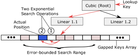
Figure 3: Example of 2-levels Gapped RMI (GRMI)

The performance of any INLJ algorithm mainly depends on the used index. However, when using RMI in INLJ over challenging inputs, the join throughput deteriorates as the input data is difficult to learn and the accuracy of built RMI becomes poor. In this case, the RMI predicts a location which is far away from the true one, and hence the overhead of searching between the error bounds becomes significant. This is because when an RMI is built for an input relation, it never changes the positions of the tuples in this relation. A key insight from a recent updatable learned index [15], namely ALEX, shows that when tuples are inserted using a learned model, the search over these tuples later, using the same model, will be improved significantly. Basically, model-based insertion places a key at the position where the model predicts that the key should be. As a result, model-based insertion reduces the model misprediction errors. This inspires us to propose a new read-only RMI-based index, namely Gapped RMI (GRMI), that substantially improves the lookup performance over typical RMI, specially for datasets with challenging distributions.

GRMI Structure. The proposed GRMI consists of a typical RMI and two gapped arrays, one for keys and one for payloads. We assume both keys and payloads have fixed sizes. Any payload could be an actual record or a pointer to a variable-sized record, stored somewhere else. The gapped arrays are filled by model-based inserts of the input tuples (described later). The extra space used for the gaps is distributed among the elements of the array, to ensure that tuples are located closely to the predicted position when possible. The number of allocated gaps per input key is a user-defined parameter that can be tuned. For efficient lookup, the gapped arrays are associated with a bitmap to indicate whether each location in the array is filled or is still a gap. Figure 3 depicts an example of a 2-levels GRMI, where we show only the gapped array for keys (white cells are gaps (i.e., empty)).

GRMI has two main differences from ALEX. First, GRMI is a read-only data structure which is built once in the beginning and then used for lookup operations only. In contrast, ALEX is more dynamic and can support updates, insertions and deletes. Second, ALEX is a B-tree-like data structure which has internal nodes containing pointers and storing intermediate gapped arrays. Unlike ALEX, GRMI just has only two continuous gapped arrays, for keys and payloads, to perform the ”last-mile” search operations in an efficient manner. Note that GRMI employs a typical RMI for predicting the key’s location, without any traversal for internal nodes as in ALEX. Therefore, the GRMI lookup is extremely efficient compared to ALEX as shown in our experiments (Section VI).

GRMI Building. Building a GRMI has two straightforward steps. First, a typical RMI is constructed for the input keys. Then, the built RMI is used to model-based insert all tuples from scratch in the gapped arrays. Note that, in INLJ, the index is assumed to be existing beforehand. This is a typical case in any DBMS where indexes (e.g., hash index, B-tree) are general-purpose and built once to serve many queries (e.g., select, join). Therefore, the GRMI building overhead has no effect on the INLJ performance.

GRMI Lookup. Given a key, the RMI is used to predict the location of that key in the gapped array of keys, then, if needed, an exponential search is applied till the actual location is found. If a key is found, we return the corresponding payload at the same location in the payloads array, otherwise return null. We use the exponential search to find the key in the neighborhood because, in GRMI, the key is likely to be very close to the predicted RMI location, and in this case, the exponential search can find this key with less number of comparison checks compared to both sequential and binary searches. Figure 3 presents a lookup example, where red arrows show the lookup flow. In this example, the RMI prediction is corrected by two exponential search steps only.

III-B Buffered GRMI INLJ

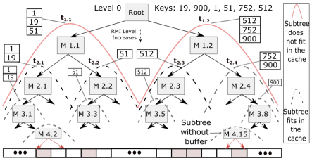
Figure 4: Example on hierarchical Request Buffers at some RMI models.

Although leveraging the model-based insertion and exponential search ideas in GRMI reduces the number of comparisons and their corresponding cache misses in the ”last-mile” search, directly using GRMI in INLJ is sub-optimal as it introduces another kind of cache misses when iteratively looking up for different keys. Since keys are stored in quite large gapped arrays in GRMI, the probability of finding different keys within the same cacheline is low. To address this issue, we propose to buffer (i.e., temporarily store) the requests for query keys that will be probably accessed from the same part in the gapped array (i.e., keys that predict the same models across the RMI levels), and then answer them as a batch. This significantly improves the temporal locality of the index, reduces cache misses, and in turn increases the join throughput. In this section, we show how we adapt an efficient variation of hierarchical buffering techniques [65, 20] to improve the throughput of INLJ using GRMI. We refer to this variation as Buffered GRMI (BGRMI).

Key Idea. We view the RMI as a tree with multiple sub-trees rooted at the child models, and the root of each sub-tree $t$ is associated with a fixed-size buffer. We refer to this buffer as request buffer, where it temporarily stores all keys that will be predicted using the corresponding child model. Any sub-tree $t$ can be recursively decomposed into smaller sub-trees at its own child models. Figure 4 shows an example of sub-trees at different levels of an RMI, where the root of each sub-tree has a request buffer. In this example, the ”Root” model has two sub-trees $t_{1.1}$ and $t_{1.2}$ rooted at its child models $M1.1$ and $M1.2$, respectively, where for example, the sub-tree $t_{1.1}$ itself has two child sub-trees $t_{2.1}$ and $t_{2.2}$ (with their buffers) rooted at the $M2.1$ and $M2.2$ models, respectively, and so on.

The request buffers for all sub-trees of the indexed relation, say $R$, are created before the INLJ begins. During the INLJ operation, the query keys from the non-indexed relation, say $S$, are distributed to the buffers based on the RMI predictions, until a buffer becomes full. When a buffer is full, we flush it by distributing the buffered query keys to its child buffers recursively (e.g., in Figure 4, when the buffer of sub-tree $t_{1.1}$ is filled with the query keys $1$, $19$, and $51$, the model $M1.1$ is then used to distribute these keys to the buffers of its child sub-trees $t_{2.1}$ and $t_{2.2}$, and so on). When a query key reaches the leaf-level, the final RMI prediction is performed. When no more query keys are issued, the whole request buffers are flushed in the depth-first order similar to [20].

During the rest of this section, we discuss how we define the size of the buffer at the root of any sub-tree $t$, and how the total size of all buffers needed for an RMI satisfies the analytical bound of the cache complexity in hierarchical indexes (e.g., trees or RMI) [20]. The cache complexity is defined by the asymptotic number of block transfers between the cache and the memory incurred by a query key.

Notation. For an RMI with a root model $r$, let $n$ be the total number of intermediate and leaf models in this RMI (without the root $r$), $m$ be the fan-out (i.e., number of children per any model in this RMI), and $w$ be the fixed-size, in bytes, of a single model in this RMI. For any sub-tree $t$ in this RMI, let $v_{t}$ be the size of the buffer associated with the ”root” model of $t$, and $g_{t}$ be the number of ”non-root” models in $t$. We also define a function $S(g_{t})$ that estimates the total size of buffers associated with the $g_{t}$ non-root models in any sub-tree $t$.

Estimating the Buffer Size $v_{t}$ at the Root of Sub-tree $t$. The buffer associated with the root of any sub-tree $t$ should consider the following two points. First, the expected number of query keys, that will be processed through $t$ and reside in the buffer at its root, depends on the number of the non-root models in $t$ (i.e., $v_{t}\propto g_{t}$). Note that $g_{t}$ is determined by the level of $t$’s root in RMI. Therefore, the closer the level of $t$’s root to the RMI root, the larger buffer size $v_{t}$ this $t$ needs (e.g., in Figure 4, the number of buffered keys in $t_{1.1}$ is larger than in either $t_{2.1}$ or $t_{2.2}$ as the level of $t_{1.1}$’s root is closer to the RMI root). Second, the buffer size $v_{t}$ at $t$’s root should be equal to (or larger than) the total size of $t$’s child sub-trees and their associated buffers (i.e., $v_{t}\geq S(g_{t})$). This is intuitive because if the child sub-trees and all their buffers fit into the cache, they can be reused before eviction from the cache. Therefore, based on these two points, we set $v_{t}$ to be $wg_{t}+S(g_{t})$, where $wg_{t}$ and $S(g_{t})$ are the total sizes of all the $g_{t}$ non-root models in $t$ and their associated buffers.

Total Buffers’ Size Upper Bound. Here, we present a worst-case bound on the total size of the request buffers needed by an RMI. Note that our goal is to maximize the INLJ performance with RMI and its variant GRMI, not to minimize the buffer sizes. Therefore, this analysis is useful for gaining intuition about request buffer sizes, but does not reflect worst-case guarantees in practice.

Proposition 1

Given an RMI with number of intermediate and leaf models $n$ (without the root), child fan-out $m$ and model size $w$, the total size, in bytes, of the request buffers at non-root models of this RMI (i.e., $S(n)$) is $O(n\log_{m}n)$.

Proof 1

As previously mentioned, an RMI with fan-out of $m$ can be viewed as a tree that starts from the root model $r$. Such tree consists of $m$ sub-trees; each sub-tree starts from one of the $m$ child models of $r$. Since the whole RMI tree contains $n$ non-root models, then each of these sub-trees roughly contains $\frac{n}{m}$ nodes. From our definitions, the total size of buffers needed for each sub-tree $t$, without the buffer needed for the root of $t$, is $S({\frac{n}{m}})$. In addition, the buffer size at the root of $t$ (i.e., $v_{t}$) is $w\frac{n}{m}+S(\frac{n}{m})$. Hence, we can redefine $S(n)$ in terms of $S(\frac{n}{m})$ to be as follows:

$$S(n)=m(w\frac{n}{m}+2S(\frac{n}{m}))=wn+2mS(\frac{n}{m})$$ (1)

By solving this equation recursively, we end up with $S(n)=wn(1+2+\ldots+\log_{m}n)+(2m)^{\log_{m}n}$, where $(1+2+\ldots+\log_{m}n)$ is a geometric series. After eliminating lower-order terms of this series and assuming $n\gg m$, $S(n)$ becomes $O(n\log_{m}n)$ ($w$ is omitted as it is constant).

The base case of Equation 1 occurs at the leaf-level (i.e., $S(0)=0$). Note that we can estimate the value of $S(g_{t})$ at any sub-tree $t$ by replacing $n$ in Equation 1 with $g_{t}$, and recursively solve the equation starting from the RMI level of the $t$’s root till the leaf. Also, note that the assumption of $n\gg m$ (used in the proof) is valid as, in practice, the RMI optimizer [47] typically models a large input relation with complex distribution using RMI of 2 to 3 levels (excluding the root), and a fan-out $m$ of 1000. In the case of 2 levels, for example, the $\frac{n}{m}$ ratio becomes 1000, which is relatively large.

Optimizing the Number of Buffers in RMI. Assigning a buffer for ”every” sub-tree in RMI is unnecessary and will result in cache misses when accessing the buffers themselves, specially in case of having large RMI (i.e., large number of buffers). Therefore, as an optimization, we keep assigning the buffers on the RMI sub-trees, level by level (starting from level 1), until a sub-tree $t$ and its buffers (excluding the buffer of this sub-tree’s root) totally fit into the cache and then stop. For example, in Figure 4, we start by assigning buffers to sub-trees $t_{1.1}$ and $t_{1.2}$ (RMI level 1). Then, we assign buffers to their child sub-trees $t_{2.1},t_{2.2},t_{2.3}$ and $t_{2.4}$ (RMI level 2). Here, we assume that $t_{2.1},t_{2.2},t_{2.3}$ and $t_{2.4}$ and the buffers at their child sub-trees (RMI level 3) can fit in the cache (highlighted with dotted lines). Therefore, we stop assigning buffers to the sub-trees at higher levels (i.e., RMI level 4).

Buffers Cache Complexity. Assume $B$ is the cache line size in bytes, and $C$ is the cache capacity in bytes. According to [20], the amortized cache complexity of one probe using the buffering scheme of a hierarchical index $X$ (e.g., trees or RMI) should be less than or equal to $O(\frac{1}{B}\log_{C}n)$, where $n$ is the number of index nodes (RMI models in our case). Otherwise, this buffering scheme is considered inefficient. Here, we show that our request buffers match the analytical bound of probing cache complexity, and hence proved to be efficient.

Proposition 2

The amortized cache complexity of one probe using our request buffers is $O(\frac{1}{B}\log_{C}n)$, where $n$ is the number of RMI models, and hence matches the analytical bound from [20].

Proof 2

As mentioned before, we apply the request buffers on the RMI index, starting from the first level, until a sub-tree $t$ and its buffers (excluding the buffer of this sub-tree’s root) totally fit into the cache. Assume the number of models in this sub-tree $t$ is $k$. Then, using Proposition 1, the total size of the sub-tree $t$ and its buffers, excluding the buffer at $t$’s root, can be represented using this inequality $w(k\log_{m}k)<C$. By taking $\log_{m}$ for both sides, $(\log_{m}k+\log_{m}\log_{m}k)<\log_{m}\frac{C}{w}$. After eliminating lower-order terms, $\log_{m}k<\log_{m}\frac{C}{w}$.

Assume the size of probe key in bytes is $q$. Since we are using fixed-size buffers, the amortized cost of each probe on a sub-tree that fits in the cache is $O(\frac{1}{B})$, because the cost of loading sub-tree into the cache is amortized among $\frac{w(k\log_{m}k)}{q}$ probes. In addition, the number of sub-trees fitting in the cache that each probe should go through is $O(\frac{\log_{m}n}{\log_{m}k})=O(\frac{\log_{m}n}{\log_{m}C})=O(\log_{C}n)$. As a result, the amortized cost of each probe on the RMI index is $O(\frac{1}{B}\log_{C}n)$, and meets the analytical bound in [20].

III-C Learned-based Hash INLJ

Instead of directly using a learned index (e.g., RMI or RadixSpline [27]) in INLJ (e.g., GRMI-INLJ), we can employ a variant of a hash index that only uses the CDF-based models, as a hash function, to build and probe a typical hash table [56] (i.e., just using the CDF-based models without storing keys in RMI-specific data structures, such as gapped arrays, or applying any buffering optimization). Basically, if the input keys are generated from a certain distribution, then the CDF of this distribution maps the data uniformly in the range $[0,1]$, and the CDF will behave as an order-preserving hash function in a hash table. In some cases, the CDF-based models can over-fit to the original data distribution, and hence result in less number of collisions compared to traditional hashing, which would still have around 36.7% regardless of the data distribution (based on the birthday paradox). For example, if the data is generated in an incremental time series fashion, or from sequential data with holes (e.g., auto generated IDs with some deletions), the predictability of the gaps between the generated elements determines the amount of collisions [56], and can be captured accurately using learned models. Note that we build the CDF-based models using the entire input relation, and hence its accuracy becomes high. Our experimental results (Section VI) show the effectiveness of the learned-based hash variant in some real and synthetic datasets.

IV Learned Sort-based Join

Sort-based join (SJ) is an essential join operation for any database engine. Although its performance is dominated by other join algorithms, like partitioned hash join [62], it is still beneficial for many scenarios. For example, if the input relations are already sorted, then SJ becomes the best join candidate as it will skip the sorting phase, and directly perform a fast merge-join only. Another scenario is applying grouping or aggregation operations (e.g., [10, 1]) on join outputs. In such situation, the query optimizer typically picks a SJ as it will generate nearly-sorted inputs for the grouping and aggregate operations. In this section, we propose an efficient learned sort-based join algorithm, namely L-SJ, which outperforms the existing state-of-the-art SJ algorithms.

IV-A Algorithm Design

One straightforward design to employ the learned models in SJ is to directly use a LearnedSort algorithm (e.g., [32]) as a black-box replacement for the sorting algorithms used in the state-of-the-art SJ techniques, such as MPSM [2] and MWAY [62]. This is an intuitive idea specially that the sorting phase is the main bottleneck in SJ, and using the LearnedSort is expected to improve the sorting performance over typical sorting algorithms as shown in [32]. However, based on our experiments, such design leads to a sub-par performance because LearnedSort is typically applied on different input partitions in parallel, and some of its processing steps (such as sampling, model building, and CDF-based partitioning) can save redundant work, if they are designed to be shared among different partitions and subsequent SJ phases.

Based on this insight, we design another SJ variant, namely L-SJ, that supports work sharing, and hence reduces the overall algorithm latency. L-SJ achieves that through building a CDF-based model that can be reused to improve the different SJ phases (e.g., sort and join) by just scaling up its prediction degree. In addition to that, L-SJ implements the good learned lessons from the SJ literature. In particular, MWAY [62] shows that using a sorting algorithm with good ability to scale up on the modern hardware, like AVX sort [4], is more desirable in a multi-core setting, even if it has a bit higher algorithmic complexity. Moreover, MPSM [2] concludes that getting rid of the merge phase increases the SJ throughput as merging is an intensive non-local write operation. L-SJ leverages these two hints along with the CDF-based model in the implementation of its phases as described in the rest of this section.

IV-B L-SJ Partition Phase

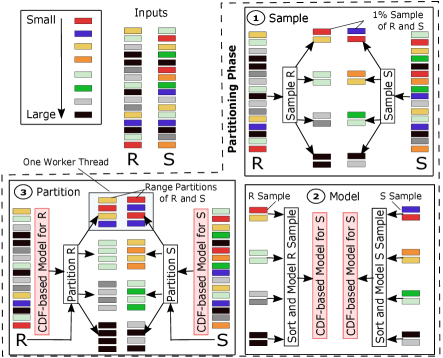
Figure 5: L-SJ partitioning phase (the color of a key reflects how large it is).

The objective of this phase is to perform a range partitioning for both $R$ and $S$ relations among the different worker threads, such that the output partitions of each relation become relatively sorted and allow the L-SJ subsequent phases to work totally in parallel (i.e., without any synchronization).

Key Idea. The partitioning idea is straightforward. We build a CDF-based model for each input relation based on a small data sample, and then use this model (instead of the traditional radix partitioning [62]) to range-partition the relation among the different worker threads. Note that we follow the partitioning theme of MWAY [62] where we range-partition both relations, not just the smaller one as in MPSM [2]. Although this makes the partitioning phase has a bit worse performance, the extra partitioning overhead is not a major bottleneck and already dominated by its effect on improving the sorting phase as described later (check Section IV-C).

Model Building. As shown in the first two steps of Figure 5, we build the model for each relation as follows: (1) in parallel, each worker samples around 1% of the input tuples, (2) the sample in each worker is then sorted, and after that, all sorted samples from the different workers are merged into one worker to train and build the model.

Range Partitioning. Inspired by [2, 62], we implement this operation (the third step in Figure 5) as follows: (1) each worker locally partitions its input chunk using the built model. While partitioning, each worker keeps track of the partitions’ sizes and builds a local histogram for the partitions at the same time, then (2) the local histograms are combined to obtain a set of prefix sums where each prefix sum represents the start positions of each worker’s partitions within the target workers, and finally (3) each worker sequentially writes its own local partitions to the target workers. Note that there is no separate step for building the local histograms, as we directly use the model to partition the data into an over-allocated array to account for skewed partitions. This approach is adapted from a previous work on the LearnedSort [32] and proves its efficiency. Typically, with a good built model, the partitions are balanced and the over-allocation overhead is 2%.

Software Write-Combine (SWWC) Buffers. To further reduce the overhead of local partitioning, we used a well-known SWWC optimization, combined with non-temporal streaming [62, 57]. Basically, SWWC reduces the TLB pressure by keeping a cache-resident buffer of entries for each partition, such that these buffers are filled first. When a buffer becomes full, its entries are flushed to the final partition. With non-temporal streaming, these buffers bypass all caches and are written directly to DRAM to avoid polluting the caches with data that will never be read again.

IV-C L-SJ Sort Phase

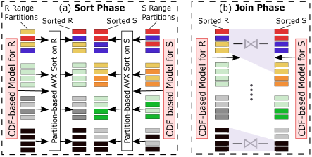
Figure 6: L-SJ sorting and joining phases (Continued example from Figure 5).

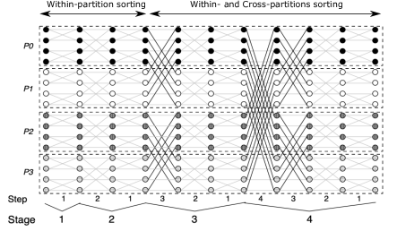
Figure 7: Example of a bitonic sorting network for 16 items with 4 partitions.

Once the partitioning phase generates the output $R$ and $S$ range partitions for the different workers, each worker sorts its own partitions locally. At the end of the sorting phase, both relations will be globally sorted and ready to be directly joined as described in Section IV-D. Typically, the sorting phase is implemented in a multi-threaded environment using an SIMD variation of the bitonic sort, namely AVX sort [4]. Although the complexity of bitonic sort is $O(n\log^{2}n)$, which is a bit higher than the standard $O(n\log n)$ complexity, the bitonic sort is better for parallel implementation on modern hardware as it compares elements using min/max instructions in a predefined sequence that never depends on the data. Here, we propose an new efficient variation of the AVX sort that exploits CDF-based partitioning to reduce its number of comparisons. We also discuss its complexity and trade-offs.

Key Idea. On each worker, the proposed AVX sort variation takes the local range partition (i.e., output of the partitioning phase (Section IV-B)) of one relation, say $R$, along with the CDF-based model of this relation as inputs (Figure 6(a)). It first uses the model to further divide the local partition into non-overlapping partitions $p$ that are relatively sorted, then apply the AVX sort on each partition independently. The number of partitions $p$ is tuned to provide a good balance between parallelism and caching performance. Note that we reuse the same CDF-based model from the partitioning phase, but we scale its prediction up for higher degree of partitioning.

Complexity Analysis. To compute the complexity of the new AVX sort, let $n$ be the number of keys to be sorted, and $p$ be the number of CDF-based partitions. Each partition has $\frac{n}{p}$ keys roughly. Figure 7 shows an example of a typical bitonic sorting network (the core of AVX sort) for 16 keys ($n=16$) and 4 partitions ($p=4$). It also highlights the type of each sorting comparison, whether it occurs within the same partition (grey arcs) or across different partitions (black arcs). As shown, the first $\log\frac{n}{p}$ stages execute completely local (within the same partition). For a subsequent stage $\log\frac{n}{p}+k$ where $1\leq k\leq\log p$, the first $k$ steps compare keys from different partitions, while the last $\log\frac{n}{p}$ steps are completely local. As mentioned before, the total complexity of typical bitonic sort is $O(n\log^{2}n)$, which is basically the total number of comparisons whether they are within the same partitions or not. However, using our proposed variation, we first need $O(n)$ for the CDF-based partitioning, and then a total of $O(\frac{1}{2}n(\log\frac{n}{p})(\log\frac{n}{p}+1))$ for the comparisons occurring in the first $\log\frac{n}{p}$ stages (within the same partition only). Note that our algorithm will skip the remaining stages as the partitions are already relatively sorted. So, the total complexity of our algorithm is $O(n+\frac{1}{2}n(\log\frac{n}{p})(\log\frac{n}{p}+1))=O(n\log^{2}\frac{n}{p})$.

Partitioning Fan-out. As shown from the complexity analysis, the number of partitions $p$ plays a key role in improving the AVX sort throughput. Increasing $p$ leads to creating more small partitions that need less number of AVX sort stages to be sorted. In addition, these partitions will fit nicely in the cache, and hence improves the temporal locality during sorting as well. On the other hand, having a large number of partitions may lead to a different type of cache problem. It may cause TLB misses if the number of created partitions is too large. We found that estimating the value of $p$ to be around 60% of the number of L1/L2 TLB entries provides a good balance between TLB misses and cache fitting.

IV-D L-SJ Join Phase

Since the two relations $R$ and $S$ become globally sorted, we skip any merge phase and directly merge-join them.

Key Idea. Assuming that $S$ is the smaller relation, the basic idea is to perform a join between each partition from $R$ and all its overlapping partitions from $S$ (Note that these partitions are the final ones generated in the sorting phase, right before applying the AVX sort).

Chunked-Join. The join operation is performed in two steps: 1) for any partition in $R$, we identify the start and the end positions of its overlapping partitions in $S$ (e.g., the first partition from $R$ only overlaps with the first two partitions from $S$ in Figure 6(b)). To do that, we query the CDF-based model of $S$ - scaled up by the same factor used in the sorting phase of $S$ to generate its partitions - with the values of the first and the last keys of this partition from $R$ to return the corresponding first and last overlapping partitions from $S$, namely $f_{S}$ and $l_{S}$, respectively. Then, 2) we merge-join any partition from $R$ with each partition in $S$ belongs to the corresponding overlapping range $[f_{S},l_{S}]$ (including $f_{S}$ and $l_{S}$) to find the final matching tuples. Note that all joins from different workers are done in parallel.

We reuse the same fine-grained partitions from the sorting phase in the join operation for two main reasons. First, this ensures using the models correctly when predicting the overlapping partitions as we reuse the same CDF scale up factor when querying the same model. Second, such partitions are probably small enough to fit in the cache (their sizes are already tuned for the AVX sort using the partitioning fan-out).

IV-E L-SJ Complexity Analysis

Assume $W$ to be the number of worker threads used to run L-SJ. Let $N_{R}$ and $N_{S}$ to be the number of tuples in relations $R$ and $S$, respectively. Let $S_{R}$ and $S_{S}$ to be the number of sampled tuples from relations $R$ and $S$, respectively, to build their CDF-based models. Also, assume $P_{R}$ and $P_{S}$ to be the total number of final sorted partitions in relations $R$ and $S$, respectively, where $P_{R}\geq W$ and $P_{S}\geq W$. Assume $O_{R}$ to be the maximum number of workers that have overlapping partitions in $R$ with any tuple in $S$ ($0\leq O_{R}\leq W$). Similarly, assume $O_{S}$ to be the maximum number of workers that have overlapping partitions in $S$ with any tuple in $R$ ($0\leq O_{S}\leq W$). We can roughly compute the complexity of L-SJ for each worker thread to be the total of the following complexities, corresponding to its different phases:

• $[\frac{S_{R}+S_{S}}{W}+S_{R}\log S_{R}+S_{S}\log S_{S}]$ (for sampling and building the CDF-based models for $R$ and $S$)

• $[\frac{N_{R}+N_{S}}{W}]$ (for range partitioning two chunks from $R$ and $S$ with sizes $\frac{N_{R}}{W}$ and $\frac{N_{R}}{S}$, respectively)

• $[\frac{N_{R}}{W}\log^{2}\frac{N_{R}}{P_{R}}+\frac{N_{S}}{W}\log^{2}\frac{N_{S}}{P_{S}}]$ (for sorting two chunks from $R$ and $S$ with sizes $\frac{N_{R}}{W}$ and $\frac{N_{S}}{W}$, respectively)

• $[\frac{N_{R}}{W}O_{S}+\frac{N_{S}}{W}O_{R}]$ (for processing two chunks from $R$ and $S$ with sizes $\frac{N_{R}}{W}$ and $\frac{N_{S}}{W}$, respectively, in the join phase)

V Learned Hash-based Join

Here, we discuss our trials to improve the performance of hash-based joins (HJ) using RMI and CDF-based partitioning (we refer to them here as learned models). Similar to learned-based hash INLJ (Section III-C), the main idea is to replace the hash functions used in both non-partitioned (NPJ) and partitioned (PJ) hash joins with learned models. Unfortunately, learned models showed a poor performance (i.e., high overall latency) in both NPJ and PJ algorithms. This is mainly because of the poor accuracy of the model used. In the case of learned-based hash INLJ, a pre-built learned index is assumed to exist on one of the input relations (i.e., indexing time is not included in the join time). Therefore, the learned models in such index can be built offline from the entire dataset to accurately capture the underlying data distribution, and have a very competitive performance with hashing. However, in the HJ algorithms, the input relations are not pre-indexed (e.g., intermediate outputs of two operators). Therefore, the learned models need to be built during the join execution, which is infeasible using the entire input relations as it will significantly increase the join latency. Therefore, we build the learned models with a small data sample (typically ranges from 1% to 10% of the input relations). This makes the model accuracy poor, and leads to inefficient hash tables building and probing in both (HJ) algorithms (Check Section VI for more evaluation results).

VI Experimental Evaluation

In this section, we experimentally study the performance of the learned and non-learned variations of indexed nested loop joins (INLJ), sort-based joins (SJ) and hash-based joins (HJ). Section VI-A describes the competitors, datasets, hardware and metrics used. Section VI-B analyzes the performance under different dataset types, sizes and characteristics. It also analyzes the joins under different threading settings and via performance counters (e.g., cache misses). Sections VI-C and  VI-D analyze the performance while tuning specific parameters for the learned INLJ and SJ algorithms, respectively.

VI-A Experimental Setup

Competitors. For INLJ, we evaluate two categories of indexes.

Learned Indexes. We provide the following three variants of RMI: (1) typical RMI (RMI-INLJ) as described in Section II-D, and both (2) gapped (GRMI-INLJ) and (3) buffered gapped RMI (BGRMI-INLJ) as described in Section III. We also provide a variant of a learned-based hash index (RSHASH-INLJ), that uses RadixSpline [27] as a hash function (described in Section III-C). We selected RadixSpline instead of RMI in this variant to explore more learned models in our experiments. Finally, we include a variant of the updatable learned index (ALEX-INLJ), that uses ALEX [15], which is very relevant to our proposed GRMI. The implementations of RMI, RadixSpline and ALEX are obtained from their open-source repositories [53, 54, 3]. The RMI hyper-parameters are tuned using CDFShop [47], an automatic RMI optimizer. RadixSpline is manually tuned by varying the error tolerance of the underlying models. ALEX is configured according to the guidelines in its published paper [15].

Non-Learned Indexes. We also report the INLJ performance with three tree-structured indexes (the Adaptive Radix Trie [38] (ART-INLJ), the Cache-Sensitive Search Trees [22] (CSS-INLJ), and a buffered variant of the Cache-Sensitive Search Tree (BCSS-INLJ), which utilizes the proposed hierarchical buffering in Section III-B), and two hash indexes (a bucket chaining hash index (HASH-INLJ), and a cuckoo hash index (CUCKOO-INLJ)). We build each index using the entire input relation (i.e., inserting every key). In addition, the implementations of tree-structured indexes are provided by their original authors, while the cuckoo hash index is adapted from its standard implementation that is used in [59].

For SJ, we compare our proposed L-SJ (Section IV) with four sort-based join baselines, coming from the stat-of-the-art algorithms MWAY and MPSM. Unless otherwise mentioned, we use the optimized variant of our proposed algorithm, referred to as BL-SJ, which includes the SWWC buffering and non-temporal streaming optimizations. For MWAY, we have two baselines: (1) an adapted variation of the original open-source implementation in [48] that works with AVX 512, referred to as MWAY-SJ (tuned its parameters according to a recent experimental study [57]), and (2) a variation of MWAY, referred to as MWAY-LS-SJ, that uses the LearnedSort algorithm [32] as a black-box in its sorting phase. Regarding MPSM, we have two baselines: (1) a best-effort implementation of the original algorithm [2] on our own (unfortunately, the original code is not available for public), referred to as MPSM-SJ, and (2) a variation of MPSM, referred to as MPSM-LS-SJ, that uses the LearnedSort algorithm [32] as a black-box in its sorting phase.

For HJ, we use the reference implementations of non-partitioned and partitioned hash joins from [48], referred to them as NP-HJ and P-HJ, respectively, and adapted two learned variations from them by replacing their hash functions with learned models, referred to them as LNP-HJ and LP-HJ. We followed the guidelines in [57] to optimize the performance of all HJ algorithms.

Datasets. We evaluate all join algorithms with real and synthetic datasets. For real datasets, we use three datasets from the SOSD benchmark [44], where we perform a self-join with each dataset. Any dataset is a list of unsigned 64-bit integer keys. We generate random 8-byte payloads for each key. The real datasets are:

• face: 200 million randomly sampled Facebook user IDs.

• osm: 800 million cell IDs from Open Street Map.

• wiki: 200 million timestamps of edits from Wikipedia.

For synthetic datasets, unless otherwise stated, we generate three datasets with different data distributions for each input relation (either $R$ or $S$). Any dataset consists of a list of 32-bit integer keys, where each key is associated with 8-byte payload. Each dataset has five size variants (in number of tuples): 16, 32, 128 and 640, and 1664 million tuples. All of them are randomly shuffled. The synthetic datasets are:

• seq_h: sequential IDs with 10% random deletes (holes).

• unif: uniform distribution, with min = 0 and max = 1, multiplied by the size, and rounded to the nearest integer.

• lognorm: lognormal distribution with $\mu=0$ and $\sigma=1$ that has an extreme skew (80% of the keys are concentrated in 1% of the key range), multiplied by the dataset size, and rounded to the nearest integer.

Hardware and Implementation. All experiments are conducted on an Arch Linux machine with 256 GB of RAM and an Intel(R) Xeon(R) Gold 6230 CPU @ 2.10GHz with Skylake micro architecture (SKX) and L3 cache of 55MiB. The machine has 2 NUMA nodes, each has 40 CPUs. All approaches are in C++, and compiled with GCC (11.1.0).

Metrics. We use the join throughput as the default metric. We define it as in [57] to be ratio of the sum of the relation sizes (in number of tuples) and the total runtime $\frac{|R|+|S|}{|runtime|}$.

Default Settings. Unless otherwise stated, all reported numbers are produced with running 32 threads. For BGRMI-INLJ, we use 4 gaps per key. To fairly compare BGRMI-INLJ with hash-based indexes, we build the hash indexes to match the gaps setting of BGRMI-INLJ by (1) using a bucket size of 4 in the block chaining index (HASH-INLJ), and (2) creating a 2-table Cuckoo hash index (CUCKOO-INLJ), where the size of these tables are 4 times the size of the input relation (i.e., load factor 25%). For both BGRMI-INLJ and BCSS-INLJ, we keep assigning buffers (as mentioned in Section III-B), starting from the first index level (root is level 0), till we find that a sub-tree (and its buffers), rooted at a model (or an index node in case of BCSS-INLJ) in level $l$, can fit in the L3 cache. Then, we stop assigning buffers to sub-trees at levels higher than $l$. For BL-SJ, we use a partitioning fan-out of 10000. For any L-SJ variant, the number of range (i.e., non-overlapping) partitions is set to the number of running threads to ensure their work independence in the sorting and joining phases. For datasets, all duplicate keys are removed to make sure that ART-INLJ properly works (a separate experiment for duplicates exists).

VI-B INLJ, SJ, and HJ Evaluation Results

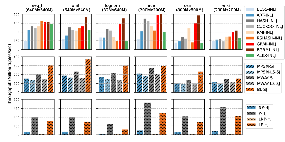
Figure 8: Performance of the three join categories for real and synthetic datasets, where each row represents a category.

Real and Synthetic Datasets. Figure 8 shows the join throughput (in million tuples per sec) of the proposed learned joins against their traditional competitors in each join category.

Clearly, BGRMI-INLJ outperforms all other INLJ competitors in all real and synthetic datasets, except seq_h. This is attributed to the effect of building the gapped RMI using ”model-based” insertion and employing the buffering optimization during key lookups. Regardless the RMI prediction accuracy for any dataset, each key is located very close to the position where it is expected to be found, and by using the exponential search, the key is typically found after 1 or 2 search steps (using binary search in RMI-INLJ takes at least 4 search steps). BGRMI-INLJ is better than GRMI-INLJ in almost all cases with a throughput improvement between 5% and 25%. RSHASH-INLJ shows a slightly better performance than BGRMI-INLJ with the seq_h dataset due to the model over-fitting in the sequential cases (Check Section III-C for more details). In contrast, RSHASH-INLJ has a very poor performance with lognorm and osm datasets. This is expected as these datasets are more skewed than others, and lead to building large sparse radix tables in RadixSpline [27]. Therefore, the learned model becomes less effective in balancing keys that will be queried in the join operation. Similarly, ALEX-INLJ suffers from the extra overhead of its B-tree-like structure. This matches the results reported by our online leaderboard [60] for benchmarking learned indexes: all updatable learned indexes are significantly slower. Unlike ALEX, the proposed GRMI variants only injected ALEX’s ideas of model-based insertion and exponential search into RMI (without internal nodes). We also found two more interesting observations. First, HASH-INLJ is slightly better than CUCKOO-INLJ. This is because, in CUCKOO-INLJ, each key has at most 2 hash table lookups (in case of having collision), which incur 2 cache misses. In contrast, the checks occurring in bucket chaining (with bucket size of 4) are mostly done on keys in the same cache line (1 cache miss). Such observation confirms the reported findings in a recent hash benchmarking study [55]. Second, the proposed hierarchical buffering in Section III-B improves the performance of INLJ with non-learned tree-structured indexes as well. In particular, BCSS-INLJ outperforms CSS-INLJ in all datasets with at least 9% (when using wiki datasets) and up to 15% (when using unif datasets) higher join throughput. Since CSS-INLJ is always the worst baseline, we removed it from all the reported results to avoid cluttered figures.

For SJ, BL-SJ consistently provides the highest join throughput in all datasets due to its effective sorting and join phases. In most datasets, BL-SJ has at least 50% and 30% less latency in the sorting and joining phases, respectively, compared to the MPSM-SJ and MWAY-SJ baselines (More breakdown results are shown in Figure 13). In addition, just replacing the sorting phase, in both MWAY and MPSM, with the LearnedSort [32] algorithm actually reduces the throughput. This is mainly because, when using the LearnedSort in SJ algorithms, its overhead becomes very significant to hide with the improvement in the sorting runtime. Assuming $W$ is the number of workers, the LearnedSort is applied $W^{2}$ times in MWAY-LS-SJ because each worker sorts $W$ local partitions before applying the multi-way merge step (i.e., sorting $W^{2}$ partitions in total from all workers). Similarly, in MPSM-LS-SJ, the overhead still exists, yet lighter (LearnedSort is repeated $W$ times only). Applying the LearnedSort many times amplifies the overhead of allocating/de-allocating its internal data structures (e.g., over-allocated and spill buckets), and hence degrades the overall throughput. In contrast to MWAY-LS-SJ and MPSM-LS-SJ, BL-SJ builds one CDF-based model for each input relation and reuses it through the partitioning, sorting and joining phases, which saves any redundant work and increases the join throughput.

For HJ, as expected, the learned variants (built with 2% samples) demonstrate very low throughputs especially for the real datasets as they are more challenging. They show at least 15X slowdown in most of the cases. Thus, we exclude the HJ results from all figures in the rest of this section.

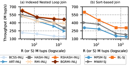
Figure 9: Performance when changing number of tuples in the seq_h dataset.

Dataset Sizes. Figure 9 shows the performance of different INLJ and SJ algorithms while scaling up the number of tuples to be joined. In this figure, we report the throughput for joining four variants of the seq_h dataset: 32Mx32M, 128Mx128M, 640Mx640M, and 1664Mx1664M (Note that the figure has a logscale on its x-axis).

For INLJ, all learned variants are able to smoothly scale to larger dataset sizes, with a small performance degradation. In case of RMI-INLJ, the ”last-mile” search step will suffer from algorithmic slowdown only as it applies binary search, and such slowdown becomes even less in the BGRMI-INLJ as it employs an exponential search instead. Moreover, both tree structures, ART-INLJ and BCSS-INLJ, become significantly ineffective at very large datasets because traversing the tree becomes more expensive compared to performing either binary or exponential search in the learned variants. For SJ, all algorithms keep the same relative performance gains regardless the sizes of input datasets.

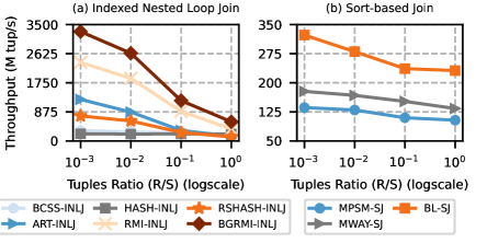
Figure 10: Performance when changing the datasets ratio (the osm dataset).

Datasets Ratio. Figure 10 shows the performance of different INLJ and SJ algorithms while joining input datasets of different sizes. In this experiment, we fix the size of one input relation $S$, which is the osm dataset with 800M tuples, while varying the number of tuples of the second input relation $R$ as a ratio from $S$. We generate four variants of the relation $R$ with the following number of tuples: 0.8M (0.1% of $S$), 8M (1% of $S$), 80M (10% of $S$), and 800M (100% of $S$). Note that the figure has a logscale on its x-axis. In case of the INLJ algorithms, we index relation $R$ to study the effect of changing the index size on the join performance.

Clearly, the throughputs of BGRMI-INLJ and RMI-INLJ at small datasets ratio, including 0.001 and 0.01, are significantly better than the throughputs of other algorithms, specially HASH-INLJ and BCSS-INLJ (at least 2X better). The main reason for that is the extremely small size of learned indexes at these ratios (compared to the tree structures and hash tables), which can completely fit into the cache (i.e., almost no cache misses). In general, the performance gap between all INLJ techniques significantly decreases at larger dataset ratios, including 0.1 and 1, where the rate of cache misses during index lookups becomes higher. We can also observe that both learned and non-learned SJ algorithms follow a similar performance trend as in INLJ algorithms, yet, with lower throughputs. This is expected as SJ includes more overhead coming from the partitioning, sorting, and merging phases (i.e., not just lookups during the join operation as in INLJ).

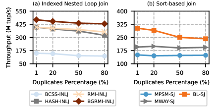
Figure 11: Performance when changing number of duplicates in the seq_h dataset.

Duplicates. Here, we study the performance of the INLJ and SJ algorithms while changing the ratio of duplicate keys in input datasets (i.e., covering 1-to-$m$ and $n$-to-$m$ joins). In this experiment, given a percentage of duplicates $x$%, we replace $x$% of the unique keys in each 640M seq_h dataset with repeated keys. Our L-SJ naturally supports joining duplicates through the Chunked-Join operation (Section IV-D). To support joining duplicates in BGRMI-INLJ, we perform a range scan between the error boundaries provided by RMI around the predicted location, similar to [44].

As shown in Figure 11, the number of duplicates affects the join throughput of our learned algorithms as the built models will always predict the same position/partition to the key, which increases the number of collisions. However, the performance of learned algorithms degrade gracefully and still remains better than non-learned algorithms. Note that the throughputs of BCSS-INLJ and HASH-INLJ are decreased as well due to the increase in their tree depth and bucket chain, respectively, while MPSM and MWAY are almost not affected.

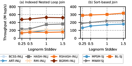
Figure 12: Performance when changing the skewness in the lognorm dataset.

Skewness. In this experiment, we study the robustness of different INLJ and SJ algorithms while changing the skewness degree of input datasets. Figure 12 shows the throughput for joining lognorm datasets, where one input relation is fixed and the other one is varied according to the skewness degree (i.e., $\sigma$). As a fixed relation, we use the lognorm dataset with 32M tuples that was generated using the default parameters mentioned in Section VI-A. For the varied relation, we generate four new lognorm datasets, each contains 640M tuples, yet, with different $\sigma$ values: 0.25, 0.5, 1 and 1.5. We index the varied relation when using the INLJ algorithms.

As shown in the figure, all algorithms show pretty similar performance at $\sigma$ values of 1 and 1.5, except BL-SJ which has a bit better throughput. However, the difference in performance becomes significant at $\sigma$ values of 0.5 and 0.25 (i.e., extremely skewed datasets). In case of the INLJ algorithms, all learned variants are less susceptible to changing the skewness degree, except RSHASH-INLJ. This is due to the ability of CDF-based learned models to balance keys over the index array, and avoid generating extremely large clusters of keys. As expected, RSHASH-INLJ has less join throughput because increasing the skewness degree (i.e., decreasing the $\sigma$ value) will increase the sparsity of the generated radix tables in RadixSpline [27], and hence leads to large clusters of keys. On the other side, the throughputs of BCSS-INLJ and HASH-INLJ are significantly decreased by increasing the skewness degree due to the increase in their tree depth and bucket chains, respectively. In case of the SJ algorithms, MPSM-SJ is the most affected algorithm by increasing the skewness degree because its range partitioning technique can easily result in unbalanced partitions among different worker threads (i.e., some threads will perform much work than others), which increases the overall algorithm latency. In contrast, BL-SJ and MWAY-SJ are almost not affected. This is because BL-SJ employs a CDF-based learned model to perform the range partitioning, and hence the work is balanced among different threads. In addition, MWAY-SJ implements a specific strategy to handle extremely large tasks (i.e., avoiding heavy hitters), which decreases the effect of skewness [4].

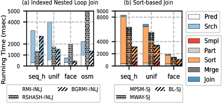
Figure 13: Runtime breakdown for the phases of learned INLJ and SJ algorithms.

Performance Breakdown. Figure 13 shows the runtime breakdown (in msec) for the different INLJ and SJ algorithms when joining different datasets. For synthetic datasets (seq_h and unif), we show the results of joining the 640Mx640M variant. For the learned INLJ case, we breakdown the runtime into RMI prediction (Pred) and final ”last-mile” search (Srch) phases. Since RSHASH-INLJ does not apply a final search step (it just uses the RadixSpline prediction as a hash value), we consider its total time as prediction (i.e., ”0” search phase). For all datasets, except seq_h, the search phase of BGRMI-INLJ is at least 3 times faster than typical RMI-INLJ, while the prediction time is almost the same.

For the SJ case, we breakdown the runtime into sampling (Smpl), partitioning (Part), sorting (Sort), merging (Mrge), and finally, merge-joining (Join). Clearly, the sorting phase is dominating in each algorithm, and improving it will significantly boost the SJ performance. On average, BL-SJ has a 3X and 2X faster sorting phase compared to MPSM and MWAY, respectively. Also, the BL-SJ joining phase is at least 1.7X faster than its counterparts in MPSM and MWAY.

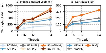
Figure 14: Performance when changing number of threads.

Parallelism. Figure 14 shows the performance of different INLJ and SJ algorithms while scaling up the number of threads from 4 to 64. In this experiment, we report the throughput for joining the 640Mx640M variant of the seq_h dataset.

Overall, all INLJ and SJ algorithms scale well when increasing the number of threads, although only the learned join variants of INLJ achieve a slightly higher throughput than others. The main explanation for this good performance is that learned INLJ variants usually incur less cache misses (Check the performance counters results in Figure 15), because they use learned models that have small sizes and can nicely fit in the cache. Since threads will be latency bound waiting for access to RAM, then threading in typical INLJ algorithms will be more affected with latency than learned variants, and degrades its performance. This observation is confirmed by a recent benchmarking study for learned indexes [44].

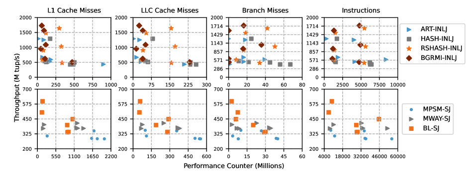
Figure 15: Low-level performance counters for exploratory analysis, where each row represents a category of join.

Other Performance Counters. To better understand the behavior of the proposed learned join algorithms, we dig deep into their low-level performance counters, and try to find any correlation between these counters and the join throughput. Figure 15 presents the plotting of four performance counters (in millions) for different INLJ and SJ algorithms, where each column represents a counter type and each row represents a join category. For INLJ, we can see that most of the BGRMI-INLJ cases with high join throughputs occur at low cache misses, whether L1 or LLC. This is explainable as most of such misses happen in the ”last-mile” search phase (a typical 2-levels RMI will have at most 2 cache misses in its prediction phase, hopefully only 1 miss if the root model is small enough), and hence improving it by reducing the number of search steps will definitely reduce the total cache misses. For other counters, it seems that there is no obvious correlation between their values and the join throughput.

In contrast, for SJ, there is a clear correlation between the BL-SJ’s counter values and the corresponding join throughput. The BL-SJ throughput increases by decreasing the number of cache and branch misses. This is mainly because the AVX sort is applied on small partitions that have better caching properties. In addition, the number of comparisons in the AVX sort itself becomes lower (Check the sorting phase complexity in Section IV-C), which in turn, reduces the number of branch misses as well.

VI-C INLJ-Specific Evaluation Results

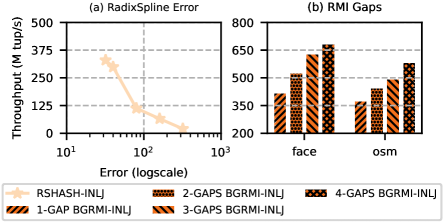
Figure 16: Effect of changing RadixSpline error and RMI gap settings on the performance of RSHASH-INLJ and BGRMI-INLJ, respectively.

RadixSpline Error. Tuning the user-defined error value is an essential step for boosting the RadixSpline performance [27]. Figure 16(a) shows how the throughput of RSHASH-INLJ is affected while changing the RadixSpline error value (Note that the figure has a logscale on its x-axis). Here, we self-join the wiki dataset. In general, increasing the error value will lead to more relaxed models with higher misprediction rate, which in turn build a hash table with higher collision rate.

RMI Gaps. Figure 16(b) shows the effect of increasing the number of gaps assigned per key in BGRMI-INLJ, while self-joining each of the face and osm datasets. As expected, increasing the gaps degree allows for more space around each key to handle mispredictions efficiently, which in turn reduces the final search steps and increases the throughput. However, having more gaps will come with higher space complexity as well. Thus, this parameter needs to be tuned carefully.

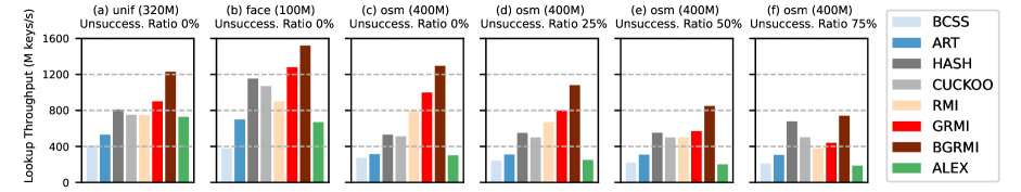
Figure 17: Performance of the GRMI and BGRMI indexes compared to others, while changing the lookup workload sizes and unsuccessful ratios.

Index Lookup. In this experiment, we focus on studying the effectiveness of both GRMI and BGRMI (compared to existing solutions) as general lookup indexes. Figure 17 shows the index lookup throughput in million keys per sec (y-axis) while changing the lookup workload. In the left three subfigures, we build indexes for the whole keys in the unif, face and osm datasets. Then, we generate a lookup workload from each dataset by randomly selecting, with replacement, 50% of the indexed keys (i.e., all lookup keys already exist in the index, i.e., unsuccessful lookup ratio of 0%). In the right three subfigures, we reuse the built osm indexes before, yet, we change the osm lookup workload by randomly replacing 25%, 50% and 75% of its keys with non-existing ones to have three more osm lookup workloads with unsuccessful ratios of 25%, 50% and 75%, respectively. We build all indexes with the same default settings mentioned in Section VI-A. Interestingly, the performance gap between the traditional RMI and our proposed variants, i.e., GRMI and BGRMI, decreases by increasing the the ratio of unsuccessful lookups (GRMI becomes even worse than RMI at unsuccessful lookup ratio of 75%). This is because both GRMI and BGRMI perform the ”last-mile” search using the exponential search (instead of the binary search used in RMI), which is not the best solution when the search key is unlikely to be among the first neighbours around the model prediction. That being said, BGRMI still has the best lookup performance in all cases as it combines both the model-based insertion idea and the hierarchical buffering optimization. We also observe that the advantage of HASH (i.e., bucket chaining) over CUCKOO becomes more significant at higher unsuccessful lookup ratios as well. This is due to the same reason mentioned before in Figure 8: using CUCKOO (with 2 hash tables) guarantees 2 cache misses per each unsuccessful lookup, yet, HASH will probably do the required checks within the same cacheline (i.e., 1 cache miss). Finally, although BCSS is equipped with the hierarchical buffering optimization, its performance is still greatly penalized by the need to traverse the increased tree depths, specially in large datasets.

VI-D SJ-Specific Evaluation Results

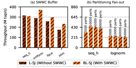
Figure 18: Effect of changing SWWC buffer and partitioning fan-out settings on the performance of L-SJ.

SWWC Buffer. Figure 18(a) shows the effect of enabling the SWWC buffering on the performance of L-SJ while joining different datasets. For synthetic datasets (seq_h and unif), we show the results of joining the 640Mx640M variant. We can see that most datasets benefit from enabling buffering in the partitioning phase. However, such benefit is capped by the contribution of partitioning time to the overall SJ time (typically, the partitioning phase ranges from 20% to 35% of the total time). For these datasets, except seq_h, the throughput improvement ranges from 10% to 30%.

Partitioning Fan-out. Figure 18(b) shows the effect of choosing different fan-out values (2000, 10000, 40000, and 60000) on the throughput of BL-SJ, while joining the 128Mx128M variant of seq_h and lognorm datasets. The results show that there is a sweet spot where the fan-out value hits the highest join throughput. This is expected because having a small fan-out will keep the number of comparisons in AVX sort large. In contrast, having a large fan-out will increase the TLB pressure when accessing the output partitions.

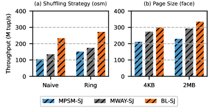
Figure 19: Effect of changing data shuffling strategy (NUMA) and page sizes (TLB entries) on the performance of the SJ algorithms.

Data Shuffling. In this experiment, we study how equipping the SJ algorithms with NUMA awareness can affect the join throughput. A recent study [40] showed that the implementation details of data shuffling across different NUMA nodes can substantially impact the interconnect bandwidth, and hence the overall performance. Since data shuffling is an essential operation in any SJ algorithm, optimizing the shuffling strategy is expected to improve the join throughput. Basically, both BL-SJ and MPSM-SJ perform data shuffling during their partitioning and joining phases, while the shuffling in MWAY-SJ occurs in its partitioning and multi-way merge phases. Here, we experiment with two data shuffling strategies: (1) Naive shuffling (the default strategy in all algorithms), which does not consider the NUMA characteristics and lets each thread pull/write data generated by all other threads without any optimization, and (2) Ring shuffling, which executes the shuffling operation on multiple steps, as described in [40], to reduce the NUMA interconnect contention. Figure 19(a) shows how the join throughputs of different SJ algorithms change under these two shuffling strategies while using the osm dataset. As expected, all algorithms benefit from the ”Ring” shuffling strategy, where the improvement ratios of join throughput are 17%, 30% and 45% for BL-SJ, MWAY-SJ and MPSM-SJ, respectively. As observed, BL-SJ has the least improvement ratio. Generally speaking, the effect of using the ”Ring” strategy becomes significant if it is used in a time-consuming phase, and vice versa. Therefore, since the partitioning and joining phases of BL-SJ do not represent more than 15% of the total algorithm time, the BL-SJ’s throughput improvement due to using the ”Ring” strategy becomes limited compared to MPSM-SJ and MWAY-SJ.

Page Size. Figure 19(b) shows the effect of changing the page size from 4KB (the default value in Unix operating systems) to a larger size 2MB (a.k.a huge page) while using the face dataset. Compared to the INLJ algorithms, SJ algorithms perform larger amount of random memory accesses (specially when having big working sets, i.e., large datasets), which can be limited by the TLB misses. We can reduce such misses by utilizing larger page sizes as suggested in previous studies (e.g., [57]). As shown in the figure, all SJ algorithms benefit from increasing the page size. Specifically, the throughputs of BL-SJ, MWAY-SJ and MPSM-SJ improved by 13%, 7%, 8%, respectively. We can observe that the improvement ratio in BL-SJ is higher than in other algorithms. This is because the overhead of the partitioning phase in BL-SJ is a bit higher (check Section IV-B), and hence reducing the TLB misses will have a greater impact. We skipped reporting the results using larger page sizes (e.g., 1GB), because there were no throughput improvement as the working set already fits in the TLB when using 2MB pages.

VII Discussion

In this section, we discuss some performance aspects and limitations related to the learned in-memory joins.

Duplicates. Having duplicate keys in the input datasets results in building imprecise CDF-based models that will lead to predicting the same position/partition for multiple keys. This increases the number of collisions, and hence reduces the join throughput (e.g., in INLJ, collisions increase the ”last-mile” search overhead, while in L-SJ, they result in imbalanced partitions that increase the sorting and joining latency). Although our experimental results (Figure 11) show the competitiveness of learned INLJ and SJ variants when having a high number of duplicates, their performance gain over non-learned variants becomes insignificant at extreme duplicate ratios (e.g., 80% or more). As a future work, we plan to employ efficient ideas from [33] to further reduce the effect of duplicates.

Complex Distributions. In general, learned joins are favorable when inputs datasets have skewed and/or complex distributions (e.g., lognorm, osm and wiki datasets). That being said, if the datasets never preserve local structure (e.g., high randomization and spikes), then the distributions of such datasets are difficult to model. In these cases, learned join variants require a significant large number of models (i.e., higher storage overhead and cache misses) to achieve errors comparable to those observed on the easy-to-learn datasets.

Vectorization. SIMD has been heavily studied in the data management field to accelerate different operations, including scanning [35, 16], bloom filters [51], non-learned joins [18, 17, 36] and sorting [13, 24]. A recent study [56] showed that, with the help of vectorization and prefetching-optimized inter-task parallelism (e.g., AMAC [28]), the prediction time of learned models can be further improved for indexing applications. We expect that employing the vectorization in learned joins will be beneficial as well, and investigating it is an interesting future research direction.

VIII Related Work

Nested Loop Joins (NLJ). Due to their simplicity and good performance in many cases, nested loop joins are widely used in database engines for decades [23]. They have been extensively studied against other join algorithms either on their own (e.g., [11]) or within the query optimization context (e.g., [37]). Block and indexed nested loop joins are the most popular variants [20]. Several works revisited their implementations to improve the performance for hierarchical caching (e.g., [20]) and modern hardware (e.g., GPU [22]).

Sort-based Joins (SJ). Numerous algorithms have been proposed to improve the performance of sort-based joins over years. However, we here highlight the parallel approaches as they are the most influential ones [25, 2, 4, 57, 7]. [25] provided the first evaluation study for sort-based join in a multi-core setting, and developed an analytical model for the join performance that predicted the cases where sort-merge join would be more efficient than hash joins. After that, MPSM [2] was proposed to significantly improve the performance of sort-based join on NUMA-aware systems. Multi-Way sort-merge join (we refer to it as MWAY) is another state-of-the-art algorithm [4] that improved over [25] by using wider SIMD instructions and range partitioning to provide efficient multi-threading without heavy synchronization.

Hash-based Joins (HJ). In general, hash-based joins are categorized into non-partitioned (e.g., [62, 8, 34]) and partitioned (e.g., [62, 57, 6]) hash joins. Radix join [9, 41, 42, 62, 5] is the most widely-used partitioned hash join due to its high throughput and cache awareness (e.g., avoiding TLB misses). [25, 8] provided first parallel designs for radix hash joins, while [62] and [6] added software write-combine buffers (SWWC) and bloom filter optimizations, respectively, to these implementations. Other works optimized the performance of hash join algorithms for NUMA-aware systems (e.g., [34, 57]), hierarchical caching (e.g., [21]), and special hardware (e.g.,GPU [22], FPGA [12], NVM [58]).

Machine Learning for Database. During the last few years, machine learning started to have a profound impact on automating the core database functionality and design decisions. Along this line of research, a corpus of works studied the idea of replacing traditional indexes with learned models that predict the location of a key in a dataset including single-dimension (e.g., [31, 27, 19]), multi-dimensional (e.g., [49, 14]), updatable (e.g., [15]), and spatial (e.g., [39, 52, 50]) indexes. Query optimization is also another area that has several works on using machine learning to either entirely build an optimizer from scratch (e.g., [46]), or provide an advisor that improves the performance of existing optimizers (e.g., [45, 61, 63]). Moreover, there exists several workload-specific optimizations, enabled by machine learning, in other database operations e.g., cardinality estimation [26], data partitioning [64], sorting [32], and scheduling [43]. However, to the best of our knowledge, there is no existing work on using the machine learning to improve in-memory joins. Our proposed work in this paper fills this gap.

IX Conclusion

In this paper, we discussed and experimentally investigated the usage of CDF-based partitioning and learned indexes (e.g., RMI and RadixSpline) in the three join categories; indexed nested loop join (INLJ), sort-based joins (SJ) and hash-based joins (HJ). We found that learned models can not improve the performance of HJ, yet, they are beneficial for INLJ and SJ. However, directly integrating learning models with INLJ and SJ leads to a sub-par performance. Therefore, we proposed optimized INLJ and SJ variants that properly exploit these learned models. In INLJ category, we introduced learned INLJs that employ efficient model-based insertion and cache-optimized buffering techniques. In SJ category, we proposed a new sort-based join, namely L-SJ, that exploits a CDF-based model to improve the different SJ phases (e.g., sort and join) by just scaling up its prediction degree. Our experimental evaluation showed that learned INLJ can be 2.7X faster than hash-based INLJ in many scenarios and with different datasets. In addition, the proposed L-SJ can be 2X faster than Multi-way sort-merge join [4], which is the best sort-based join baseline in the literature.

References

- [1] Sameet Agarwal, Rakesh Agrawal, Prasad M. Deshpande, Ashish Gupta, Jeffrey F. Naughton, Raghu Ramakrishnan, and Sunita Sarawagi. On the Computation of Multidimensional Aggregate. In Proceedings of the International Conference on Very Large Data Bases, VLDB, 1996.
- [2] Martina-Cezara Albutiu, Alfons Kemper, and Thomas Neumann. Massively Parallel Sort-Merge Joins in Main Memory Multi-Core Database Systems. In Proceedings of the International Conference on Very Large Data Bases, VLDB, 2012.
- [3] ALEX: An Updatable Adaptive Learned Index. https://github.com/microsoft/ALEX.
- [4] Cagri Balkesen, Gustavo Alonso, Jens Teubner, and M. Tamer Özsu. Multi-Core, Main-Memory Joins: Sort vs. Hash Revisited. In Proceedings of the International Conference on Very Large Data Bases, VLDB, 2013.
- [5] Cagri Balkesen, Jens Teubner, Gustavo Alonso, and M. Tamer Ozsu. Main-Memory Hash Joins on Modern Processor Architectures. IEEE Transactions on Knowledge and Data Engineering, TKDE, 27(7):1754–1766, 2015.
- [6] Maximilian Bandle, Jana Giceva, and Thomas Neumann. To Partition, or not to Partition, That is the Join Question in a Real System. In Proceedings of the ACM International Conference on Management of Data, SIGMOD, 2021.
- [7] Claude Barthels, Ingo Müller, Timo Schneider, Gustavo Alonso, and Torsten Hoefler. Distributed Join Algorithms on Thousands of Cores. In Proceedings of the International Conference on Very Large Data Bases, VLDB, 2017.
- [8] Spyros Blanas, Yinan Li, and Jignesh M. Patel. Design and Evaluation of Main Memory Hash Join Algorithms for Multi-Core CPUs. In Proceedings of the ACM International Conference on Management of Data, SIGMOD, 2011.
- [9] Peter A. Boncz, Stefan Manegold, and Martin L. Kersten. Database Architecture Optimized for the New Bottleneck: Memory Access. In Proceedings of the International Conference on Very Large Data Bases, VLDB, 1999.
- [10] Surajit Chaudhuri and Kyuseok Shim. Including Group-By in Query Optimization. In Proceedings of the International Conference on Very Large Data Bases, VLDB, 1994.
- [11] Mingxian Chen and Zhi Zhong. Block Nested Join and Sort Merge Join Algorithms: An Empirical Evaluation. In Advanced Data Mining and Applications, 2014.
- [12] Xinyu Chen, Yao Chen, Ronak Bajaj, Jiong He, Bingsheng He, Weng-Fai Wong, and Deming Chen. Is FPGA Useful for Hash Joins? Exploring Hash Joins on Coupled CPU-FPGA Architecture. In Proceedings of the International Conference on Innovative Data Systems Research, CIDR, 2020.
- [13] Jatin Chhugani, Anthony D. Nguyen, Victor W. Lee, et al. Efficient Implementation of Sorting on Multi-Core SIMD CPU Architecture. In Proceedings of the International Conference on Very Large Data Bases, VLDB, 2008.
- [14] Jialin Ding et al. Tsunami: A Learned Multi-Dimensional Index for Correlated Data and Skewed Workloads. In Proceedings of the International Conference on Very Large Data Bases, VLDB, 2020.
- [15] Jialin Ding, Umar Farooq Minhas, Jia Yu, Chi Wang, Jaeyoung Do, Yinan Li, Hantian Zhang, Badrish Chandramouli, Johannes Gehrke, Donald Kossmann, David Lomet, and Tim Kraska. ALEX: An Updatable Adaptive Learned Index. In Proceedings of the ACM International Conference on Management of Data, SIGMOD, 2020.
- [16] Markus Dreseler, Jan Kossmann, Johannes Frohnhofen, et al. Fused Table Scans: Combining AVX-512 and JIT to Double the Performance of Multi-Predicate Scans. In IEEE ICDE Workshops, 2018.
- [17] Zhuhe Fang, Zeyu He, Jiajia Chu, and Chuliang Weng. SIMD Accelerates the Probe Phase of Star Joins in Main Memory Databases. In Database Systems for Advanced Applications, 2019.
- [18] Zhuhe Fang, Beilei Zheng, and Chuliang Weng. Interleaved Multi-Vectorizing. In Proceedings of the International Conference on Very Large Data Bases, VLDB, 2019.
- [19] Paolo Ferragina and Giorgio Vinciguerra. The PGM-Index: A Fully-Dynamic Compressed Learned Index with Provable Worst-Case Bounds. In Proceedings of the International Conference on Very Large Data Bases, VLDB, 2020.
- [20] Bingsheng He and Qiong Luo. Cache-Oblivious Nested-Loop Joins. In Proceedings of the International Conference on Information and Knowledge Management, CIKM, 2006.
- [21] Bingsheng He and Qiong Luo. Cache-Oblivious Query Processing. In Proceedings of the International Conference on Innovative Data Systems Research, CIDR, 2007.
- [22] Bingsheng He, Ke Yang, Rui Fang, Mian Lu, Naga Govindaraju, Qiong Luo, and Pedro Sander. Relational Joins on Graphics Processors. In Proceedings of the ACM International Conference on Management of Data, SIGMOD, 2008.
- [23] Joseph M. Hellerstein, Michael Stonebraker, and James Hamilton. Architecture of a Database System. Found. Trends Databases, 1(2):141–259, 2007.
- [24] Hiroshi Inoue and Kenjiro Taura. SIMD- and Cache-Friendly Algorithm for Sorting an Array of Structures. In Proceedings of the International Conference on Very Large Data Bases, VLDB, 2015.
- [25] Changkyu Kim, Tim Kaldewey, Victor W. Lee, Eric Sedlar, Anthony D. Nguyen, Nadathur Satish, Jatin Chhugani, Andrea Di Blas, and Pradeep Dubey. Sort vs. Hash Revisited: Fast Join Implementation on Modern Multi-Core CPUs. In Proceedings of the International Conference on Very Large Data Bases, VLDB, 2009.
- [26] Andreas Kipf, Thomas Kipf, Bernhard Radke, Viktor Leis, Peter A. Boncz, and Alfons Kemper. Learned Cardinalities: Estimating Correlated Joins with Deep Learning. In Proceedings of the International Conference on Innovative Data Systems Research, CIDR, 2019.
- [27] Andreas Kipf, Ryan Marcus, Alexander van Renen, Mihail Stoian, Alfons Kemper, Tim Kraska, and Thomas Neumann. RadixSpline: A Single-Pass Learned Index. In Proceedings of aiDM@SIGMOD, 2020.
- [28] Onur Kocberber et al. Asynchronous Memory Access Chaining. In Proceedings of the International Conference on Very Large Data Bases, VLDB, 2015.
- [29] Tim Kraska. Towards instance-optimized data systems. In Proceedings of the International Conference on Very Large Data Bases, VLDB, 2021.
- [30] Tim Kraska, Mohammad Alizadeh, Alex Beutel, Ed H. Chi, Ani Kristo, Guillaume Leclerc, Samuel Madden, Hongzi Mao, and Vikram Nathan. SageDB: A Learned Database System. In Proceedings of the International Conference on Innovative Data Systems Research, CIDR, 2019.
- [31] Tim Kraska, Alex Beutel, Ed H. Chi, Jeffrey Dean, and Neoklis Polyzotis. The Case for Learned Index Structures. In Proceedings of the ACM International Conference on Management of Data, SIGMOD, page 489–504, 2018.
- [32] Ani Kristo, Kapil Vaidya, Ugur Çetintemel, Sanchit Misra, and Tim Kraska. The Case for a Learned Sorting Algorithm. In Proceedings of the ACM International Conference on Management of Data, SIGMOD, 2020.
- [33] Ani Kristo, Kapil Vaidya, and Tim Kraska. Defeating Duplicates: A Re-design of the LearnedSort Algorithm. In Proceedings of the AIDB Workshop @VLDB, 2021.
- [34] Harald Lang, Viktor Leis, Martina-Cezara Albutiu, Thomas Neumann, and Alfons Kemper. Massively Parallel NUMA-Aware Hash Joins. In In-Memory Data Management and Analysis, IMDM, 2015.
- [35] Harald Lang, Tobias Mühlbauer, Florian Funke, Peter A. Boncz, Thomas Neumann, and Alfons Kemper. Data Blocks: Hybrid OLTP and OLAP on Compressed Storage Using Both Vectorization and Compilation. In Proceedings of the ACM International Conference on Management of Data, SIGMOD, 2016.
- [36] Harald Lang, Linnea Passing, Andreas Kipf, Peter Boncz, et al. Make the most out of your SIMD investments: Counter Control Flow Divergence in Compiled Query pipelines. The VLDB Journal, 29:226–238, 2020.
- [37] Viktor Leis, Andrey Gubichev, Atanas Mirchev, Peter Boncz, Alfons Kemper, and Thomas Neumann. How Good Are Query Optimizers, Really? In Proceedings of the International Conference on Very Large Data Bases, VLDB, 2015.
- [38] Viktor Leis, Alfons Kemper, and Thomas Neumann. The Adaptive Radix Tree: ARTful Indexing for Main-Memory Databases. In Proceedings of the International Conference on Data Engineering, ICDE, 2013.
- [39] Pengfei Li, Hua Lu, Qian Zheng, Long Yang, and Gang Pan. LISA: A Learned Index Structure for Spatial Data. In Proceedings of the ACM International Conference on Management of Data, SIGMOD, 2020.
- [40] Yinan Li, Ippokratis Pandis, Rene Mueller, Vijayshankar Raman, and Guy Lohman. NUMA-aware Algorithms: The Case of Data Shuffling. In Proceedings of the International Conference on Innovative Data Systems Research, CIDR, 2013.
- [41] Stefan Manegold, Peter A. Boncz, and Martin L. Kersten. What Happens During a Join? Dissecting CPU and Memory Optimization Effects. In Proceedings of the International Conference on Very Large Data Bases, VLDB, 2000.
- [42] Stefan Manegold, Peter A. Boncz, and Martin L. Kersten. Optimizing Main-memory Join on Modern Hardware. IEEE Transactions on Knowledge and Data Engineering, TKDE, 14(4):709–730, 2002.
- [43] Hongzi Mao, Malte Schwarzkopf, Shaileshh Bojja Venkatakrishnan, Zili Meng, and Mohammad Alizadeh. Learning Scheduling Algorithms for Data Processing Clusters. In Proceedings of the ACM Special Interest Group on Data Communication, SIGCOMM, pages 270 – 288, 2019.
- [44] Ryan Marcus, Andreas Kipf, Alexander van Renen, Mihail Stoian, Sanchit Misra, Alfons Kemper, Thomas Neumann, and Tim Kraska. Benchmarking Learned Indexes. In Proceedings of the International Conference on Very Large Data Bases, VLDB, 2020.
- [45] Ryan Marcus, Parimarjan Negi, Hongzi Mao, Nesime Tatbul, Mohammad Alizadeh, and Tim Kraska. Bao: Making Learned Query Optimization Practical. In Proceedings of the ACM International Conference on Management of Data, SIGMOD, 2021.
- [46] Ryan Marcus, Parimarjan Negi, Hongzi Mao, Chi Zhang, Mohammad Alizadeh, Tim Kraska, Olga Papaemmanouil, and Nesime Tatbul. Neo: A Learned Query Optimizer. In Proceedings of the ACM International Conference on Management of Data, SIGMOD, 2019.
- [47] Ryan Marcus, Emily Zhang, and Tim Kraska. CDFShop: Exploring and Optimizing Learned Index Structures. In SIGMOD (Demo), 2020.
- [48] Multi-Way Sort Merge Join. https://systems.ethz.ch/research/data-processing-on-modern-hardware/projects/parallel-and-distributed-joins.html.
- [49] Vikram Nathan, Jialin Ding, Mohammad Alizadeh, and Tim Kraska. Learning Multi-Dimensional Indexes. In Proceedings of the ACM International Conference on Management of Data, SIGMOD, 2020.
- [50] Varun Pandey, Alexander van Renen, Andreas Kipf, Ibrahim Sabek, Jialin Ding, and Alfons Kemper. The Case for Learned Spatial Indexes. In Proceedings of the AIDB Workshop @VLDB, 2020.
- [51] Orestis Polychroniou and Kenneth A. Ross. Vectorized Bloom Filters for Advanced SIMD Processors. In DaMoN, 2014.
- [52] Jianzhong Qi, Guanli Liu, Christian S. Jensen, and Lars Kulik. Effectively Learning Spatial Indices. In Proceedings of the International Conference on Very Large Data Bases, VLDB, 2020.
- [53] RadixSpline. https://github.com/learnedsystems/RadixSpline.
- [54] Recursive Model Indexes. https://github.com/learnedsystems/RMI.
- [55] Stefan Richter, Victor Alvarez, and Jens Dittrich. A Seven-Dimensional Analysis of Hashing Methods and Its Implications on Query Processing. In Proceedings of the International Conference on Very Large Data Bases, VLDB, 2015.
- [56] Ibrahim Sabek, Kapil Vaidya, Dominik Horn, Andreas Kipf, and Tim Kraska. When Are Learned Models Better Than Hash Functions? In Proceedings of the AIDB Workshop @VLDB, 2021.
- [57] Stefan Schuh, Xiao Chen, and Jens Dittrich. An Experimental Comparison of Thirteen Relational Equi-Joins in Main Memory. In Proceedings of the ACM International Conference on Management of Data, SIGMOD, 2016.
- [58] Anil Shanbhag, Nesime Tatbul, David Cohen, and Samuel Madden. Large-Scale in-Memory Analytics on Intel Optane DC Persistent Memory. In Proceedings of the International Workshop on Data Management on New Hardware, DaMoN, 2020.
- [59] SOSD. https://github.com/learnedsystems/SOSD.
- [60] SOSD Leaderboard. https://learnedsystems.github.io/SOSDLeaderboard/leaderboard/.
- [61] Michael Stillger, Guy M. Lohman, Volker Markl, and Mokhtar Kandil. LEO - DB2’s LEarning Optimizer. In Proceedings of the International Conference on Very Large Data Bases, VLDB, pages 19 – 28, 2001.
- [62] Jens Teubner, Gustavo Alonso, Cagri Balkesen, and M. Tamer Ozsu. Main-Memory Hash Joins on Multi-Core CPUs: Tuning to the Underlying Hardware. In Proceedings of the International Conference on Data Engineering, ICDE, 2013.
- [63] Gary Valentin, Michael Zuliani, Daniel C. Zilio, Guy M. Lohman, and Alan Skelley. DB2 Advisor: An Optimizer Smart Enough to Recommend its Own Indexes. In Proceedings of the International Conference on Data Engineering, ICDE, pages 101 – 110, 2000.
- [64] Zongheng Yang, Badrish Chandramouli, Chi Wang, Johannes Gehrke, Yinan Li, Umar Farooq Minhas, Per Åke Larson, Donald Kossmann, and Rajeev Acharya. Qd-Tree: Learning Data Layouts for Big Data Analytics. In Proceedings of the ACM International Conference on Management of Data, SIGMOD, 2020.
- [65] Jingren Zhou and Kenneth A. Ross. Buffering Accesses to Memory-Resident Index Structures. In Proceedings of the International Conference on Very Large Data Bases, VLDB, 2003.