J01020100-7122208: an accreted evolved blue straggler that wasn’t ejected from a supermassive black hole

Abstract

J01020100-7122208 is a star whose origin and nature still challenges us. It was first believed to be a yellow super giant ejected from the Small Magellanic Cloud, but it was more recently claimed to be a red giant accelerated by the Milky Way’s central black hole. In order to unveil its nature, we analysed photometric, astrometric and high resolution spectroscopic observations to estimate the orbit, age, and 16 elemental abundances. Our results show that this star has a retrograde and highly-eccentric orbit, $e=0.914_{-0.020}^{+0.016}$. Correspondingly, it likely crossed the Galactic disk at $550\;\mathrm{pc}$ from the Galactic centre. We obtained a spectroscopic mass and age of $1.09\pm 0.10$ $M_{\odot}$ and $4.51\pm 1.44$ Gyr respectively. Its chemical composition is similar to the abundance of other retrograde halo stars. We found that the star is enriched in europium, having [Eu/Fe] = 0.93 $\pm$ 0.24, and is more metal-poor than reported in the literature, with [Fe/H] = -1.30 $\pm$ 0.10. This information was used to conclude that J01020100-7122208 is likely not a star ejected from the central black of the Milky Way or from the Small Magellanic Cloud. Instead, we propose that it is simply a halo star which was likely accreted by the Milky Way in the distant past but its mass and age suggest it is probably an evolved blue straggler.

1 Introduction

Gaia (Gaia Collaboration et al., 2016) is revolutionising our understanding of the Milky Way, providing astrometric information not only for our Galaxy’s stars but also for stars from satellite galaxies. With the Gaia Early Data Release 3 (Gaia EDR3; Brown et al. 2021), it is possible to describe the detailed orbits of many stars, including J01020100-7122208. J01020100-7122208 is a star that has a velocity of 300 km s^-1 whose origin has been analysed in recent years (Neugent et al., 2018; Massey et al., 2018), yet no consensus has been reached. Understanding the nature of high-velocity stars is important because from them we can learn, for example, about how frequently encounters between stars and the central black hole of the Milky Way are (e.g. Rossi et al. 2017), as well as what is the escape velocity of the Galaxy as a function of Galactocentric radius (e.g. Piffl et al. 2014). Therefore, reaching a consensus of J01020100-7122208 is important.

This star was a serendipitous discovery. Neugent et al. (2010) carried out a study with the objective of identifying yellow stars in the direction of the Small Magellanic Cloud (SMC) based on the radial velocities (RVs) of the objects in that field. Their motivation was that by studying yellow stars it is possible to test stellar evolutionary theory which can help us to interpret the light of distant galaxies. The authors observed 496 stars using the multi-object spectrometer Hydra at Cerro Tololo 4 m telescope. They determined RVs by cross-correlating their spectra using the Ca II triplet. They then compared their results for individual stars with the mean RV of the SMC and considered that stars with RVs similar to the value of that dwarf galaxy (160 km s^-1) were candidate members. In cases where the RV results obtained using this method were inconclusive, they complemented their analysis by using the luminosity-sensitive line O I $\lambda$ 7774: stars with measurable amounts of O I $\lambda$ 7774 should be supergiants (making it possible that the objects were in the SMC) while stars without measurable O I $\lambda$ 7774 should be foreground stars from the Milky Way. With this methodology, Neugent et al. (2010) found 176 stars that were candidate members of the SMC. They found one star with an extreme heliocentric RV of about 300 km s^-1: J01020100-7122208.

Several years later, Neugent et al. (2018, hereafter Neu18) presented a more detailed spectroscopic analysis of J01020100-7122208, using one spectrum from the spectrometer Hydra at Cerro Tololo 4m telescope, one spectrum from Echelle on the du Pont 2.1 m telescope at Las Campanas Observatory and two spectra from MagE on the Las Campanas Baade 6.5m Magellan telescope. The spectra used have resolution ranging from 3000 to 45000.

In that study, the authors classified the star as a G5-8, with an effective temperature ($T_{\mathrm{eff}}$) of 4700 $\pm$ 270 K, a surface gravity ($\log g$) of 0.8, a mass of 9 $M_{\odot}$ and an age of 30 Myr. They determined the spectral type by comparing a spectrum of J01020100-7122208 with the spectra of different spectral standards, considering the strength of metal lines and the weakness of hydrogen lines. To calculate $T_{\mathrm{eff}}$ they compared de-reddened broad-band colors to model atmospheres. Finally they used Geneva evolution models to determine the mass and, as a consequence, the age of the star. With this information they concluded that J01020100-7122208 was a yellow supergiant which was likely ejected from the SMC due to a binary companion that exploded as a supernova. This would also explain its high velocity.

As soon as Gaia DR2 (Brown et al., 2018) was released, J01020100-7122208 was studied again by Massey et al. (2018, hereafter Mas18). The authors noticed that the star’s parallax was too large to be consistent with an origin in the SMC. They thus claimed that J01020100-7122208 was instead in the Galactic halo. They performed a new spectral analysis using the same spectra used in Neu18, estimating a $T_{\mathrm{eff}}$ of 4800 $\pm$ 100 K, a $\log g$ of 2.2, an age of 180 Myr, a mass of 3-4 $M_{\odot}$ and a metallicity of $\mathrm{[Fe/H]}=-0.5$. They compared these values with evolutionary tracks and concluded that the star was in the giant or early asymptotic giant branch stage, i.e. it was not a yellow supergiant. From the age and metallicity they further concluded that the star was born in the Galactic disk. After extensively discussing several different scenarios to explain the radial velocity, Mas18 concluded that J01020100-7122208 was likely ejected from the central black hole of the Milky Way. The basis for this argument was that, when Mas18 integrated the orbit of the star back in time, they found that the star passed close to the centre of the Galaxy. The authors commented that later Gaia data releases could alter this conclusion.

Now is an interesting moment to revisit the origin of this object with a new data release from Gaia (Brown et al., 2021). Furthermore, methodologies to determine ages have improved, thanks to the improved astrometry from Gaia and information from spectroscopy. Last but not least, high resolution spectra can be used to determine chemical abundances in addition to stellar parameters. The later has proven very useful to study the origins of stars in the Galaxy (Nissen & Schuster, 2010; Hawkins & Wyse, 2018; Matsuno et al., 2019; Kordopatis et al., 2020; Das et al., 2020), because different chemical elements are produced by different nucleosynthetic channels. By understanding the connection of these channels with the star formation timescales of the Galaxy and its satellites, one can shed light on the formation history of certain stars. Other works in the literature such as Hansen et al. (2016) and Hawkins & Wyse (2018) have already used chemical abundances to explore the origin of high velocity stars in the Galaxy, proving the power of using this information about stars to unveil their origins.

In this paper, we perform a detailed analysis of J01020100-7122208 with the goal of shedding light on its origin. To do so, we consider the latest Gaia data (Gaia EDR3; Brown et al. 2021) and obtain high resolution spectra to determine stellar parameters and chemical abundances of 16 elements, ages and orbital parameters. It is the first time chemical abundances are used to study this star. In Section 2 we present the data used in our work. In Section 3, we describe the analysis to calculate the orbits, age, stellar parameters and chemical abundances of J01020100-7122208, and in Section 4 we present our results. In Section 5, we discuss our findings. Finally, in Section 6 we present our conclusions.

2 Data

The astrometric and photometric information of J01020100-7122208 was taken from Gaia EDR3 and can be found in Table 1.

Figure 1: Examples of spectra. The blue spectrum at the top corresponds to J01020100-7122208 while the magenta, orange, lilac and green ones correspond to spectra of stars used to validate our spectral results.

Table 1: Properties of J01020100-7122208. Radial velocity not available in Gaia EDR3.

Property	Information
2MASS ID	J01020100-7122208
Gaia ID	4690790008835586304
R.A. (deg)	15.504 $\pm$ 0.011
Dec. (deg)	-71.373 $\pm$ 0.010
Parallax (mas)	0.105 $\pm$ 0.012
Proper motion - R.A. (mas/yr)	8.630 $\pm$ 0.017
Proper motion - Dec. (mas/yr)	-0.938 $\pm$ 0.013
G (mag)	13.36

We used two high-resolution spectra taken using the MIKE spectrograph on the Clay Telescope at Las Campanas Observatory and reduced using CarPy (Kelson, 2003), the standard pipeline for data reduction with that instrument. The first high-resolution spectrum (R $\approx$ 25 000) was observed on (UT) 2013 January 7 and has a signal-to-noise ratio (S/N) of about 100 pixel^-1. It allowed us to determine stellar parameters, chemical abundances and RV. The second spectrum was taken on (UT) 2019 August 27 and has a greater resolution of (R $\approx$ 55 000) but a S/N of only 40 pixel^-1. The second spectrum was solely used to obtain a second RV measurement and so to rule out a possible binary nature. Any variation of RV across several years might indicate that this star is part of a binary system, affecting the determination of mass and age.

In addition, we considered a sample of MIKE spectra of 7 metal-poor halo stars. These spectra have typical S/N of 100 pixel^-1 and resolution of about 40 000. The stars were used as a control sample to validate our spectral results. These stars have been selected from APOGEE DR14 (Abolfathi et al., 2018; Holtzman et al., 2018) and have been analysed by Carrillo et al, (submitted, hereafter Car21). The control sample stars satisfy 4300 K $\leq$ $\mathrm{T_{eff}}$ $\leq$ 5000 K, 0.9 $\leq$ $\log g$ $\leq$ 2.7 and -1.75 $\leq$ [Fe/H] $\leq$ -1.0. It is important for us to validate the stellar parameters of J01020100-7122208, since previous works of Neu18 and Mas18 do not agree on them.

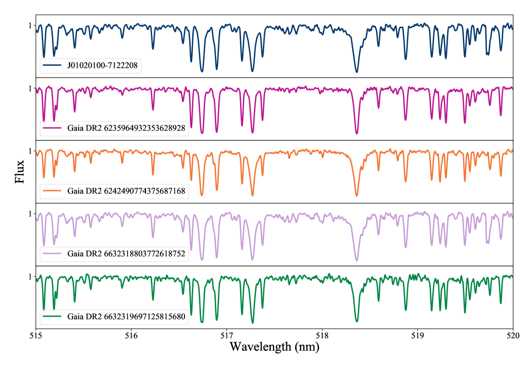
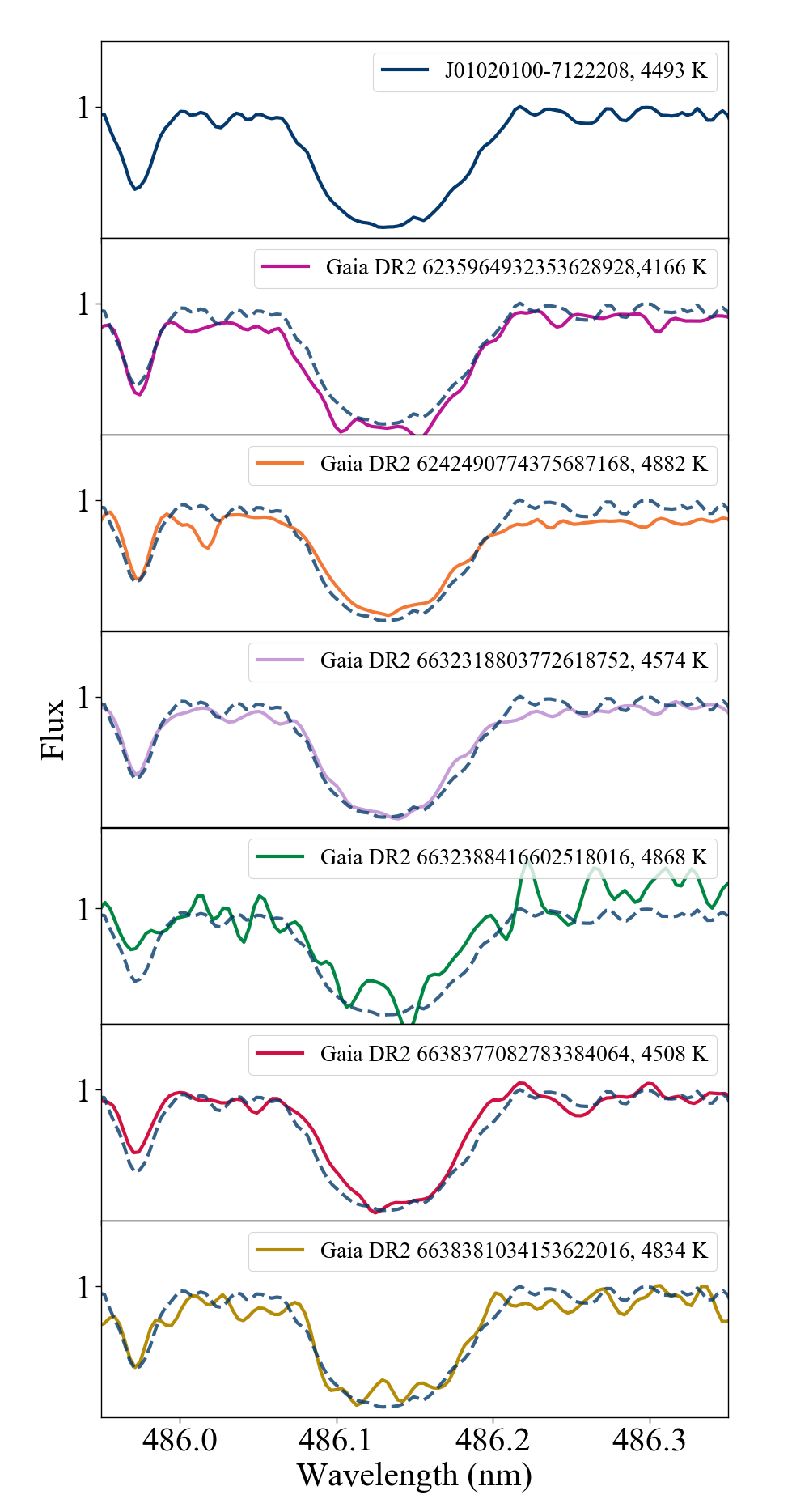
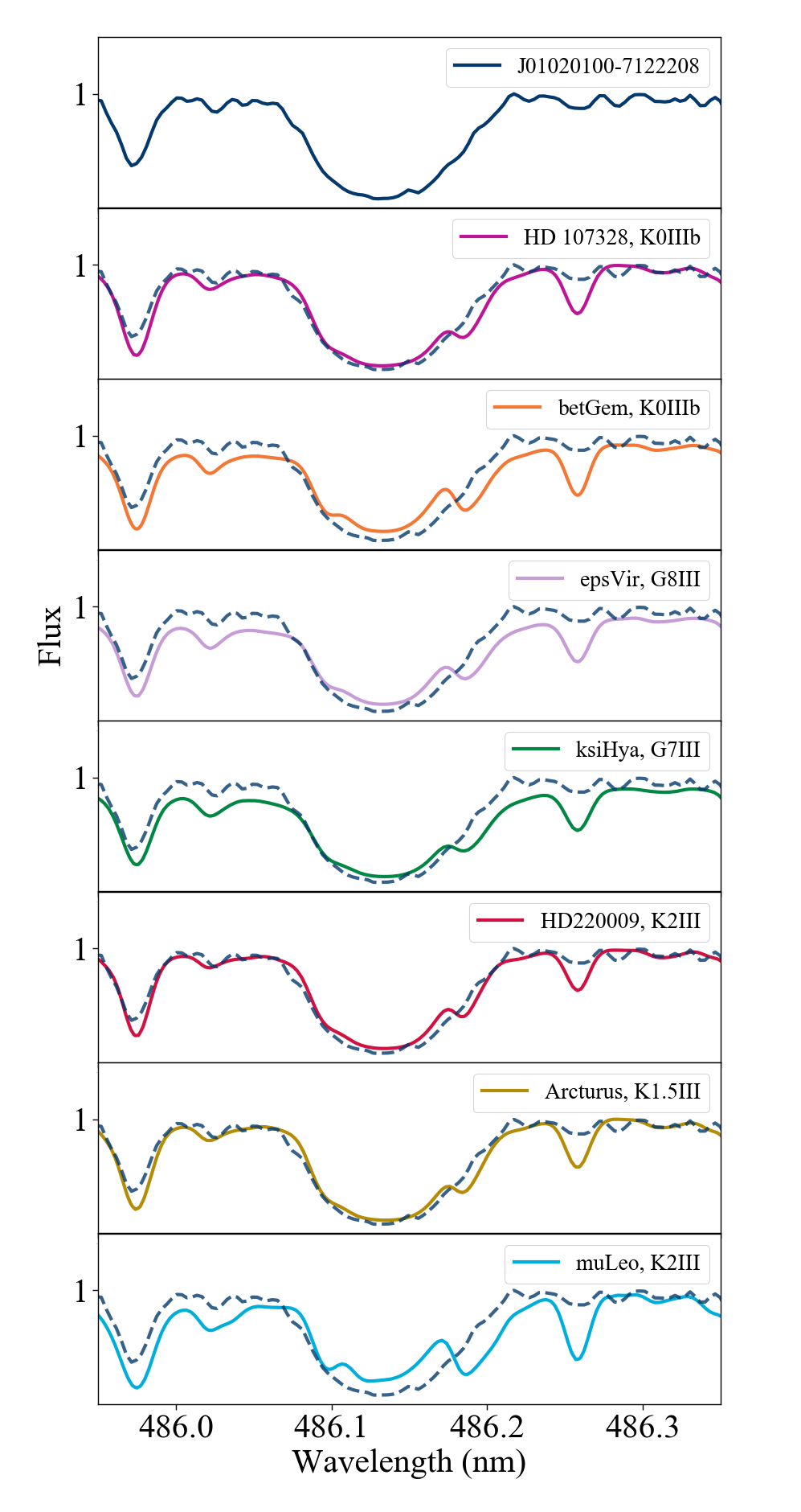
In Figure 1 we display an example region of the normalised and RV corrected spectrum of J01020100-7122208 (in blue at the top) along with 4 stars (Gaia DR2 6235964932353628928, Gaia DR2 6242490774375687168, Gaia DR2 6632318803772618752, Gaia DR2 6632319697125815680) from our control sample.

3 Analysis

3.1 Spectroscopy

We determined radial velocities, stellar parameters and chemical abundances using a pipeline developed by us based on the code for spectral analysis iSpec (Blanco-Cuaresma et al., 2014b; Blanco-Cuaresma, 2019) and IRAF tasks (Tody, 1993) were used to merge the orders of the 2D reduced spectra.

We first normalized the spectra of J01020100-7122208 and of the control sample stars order-by-order using 3-degree splines every 5 nm. We also performed the RV correction order-by-order, by cross-correlating the observed spectra with a line mask from a spectrum of Arcturus from Atlas (provided with iSpec). We did it order-by-order to avoid problems related to the wavelength calibration of our data. At this step we obtained RVs for each order. We adopted as the star’s RV the mean of the values calculated for each order and as the uncertainty the standard deviation. We visually inspected the spectra, guaranteeing that the absorption lines were aligned with the lines in the laboratory rest frame. From the spectrum acquired in 2013 we obtained a RV of 296.27 $\pm$ 0.17 km s^-1 while from the spectrum acquired in 2019 the calculated RV value is 296.24 $\pm$ 0.25 km s^-1. Both values agree within 1 sigma, therefore we find no evidence that this star is currently in a binary system.

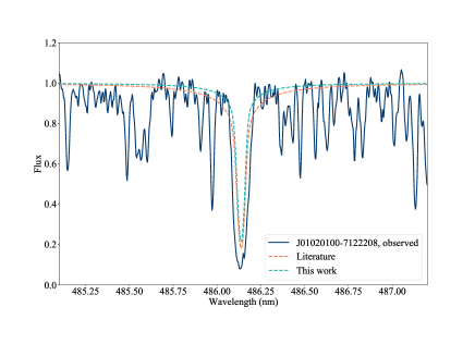
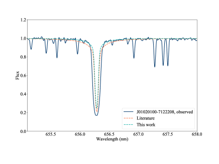
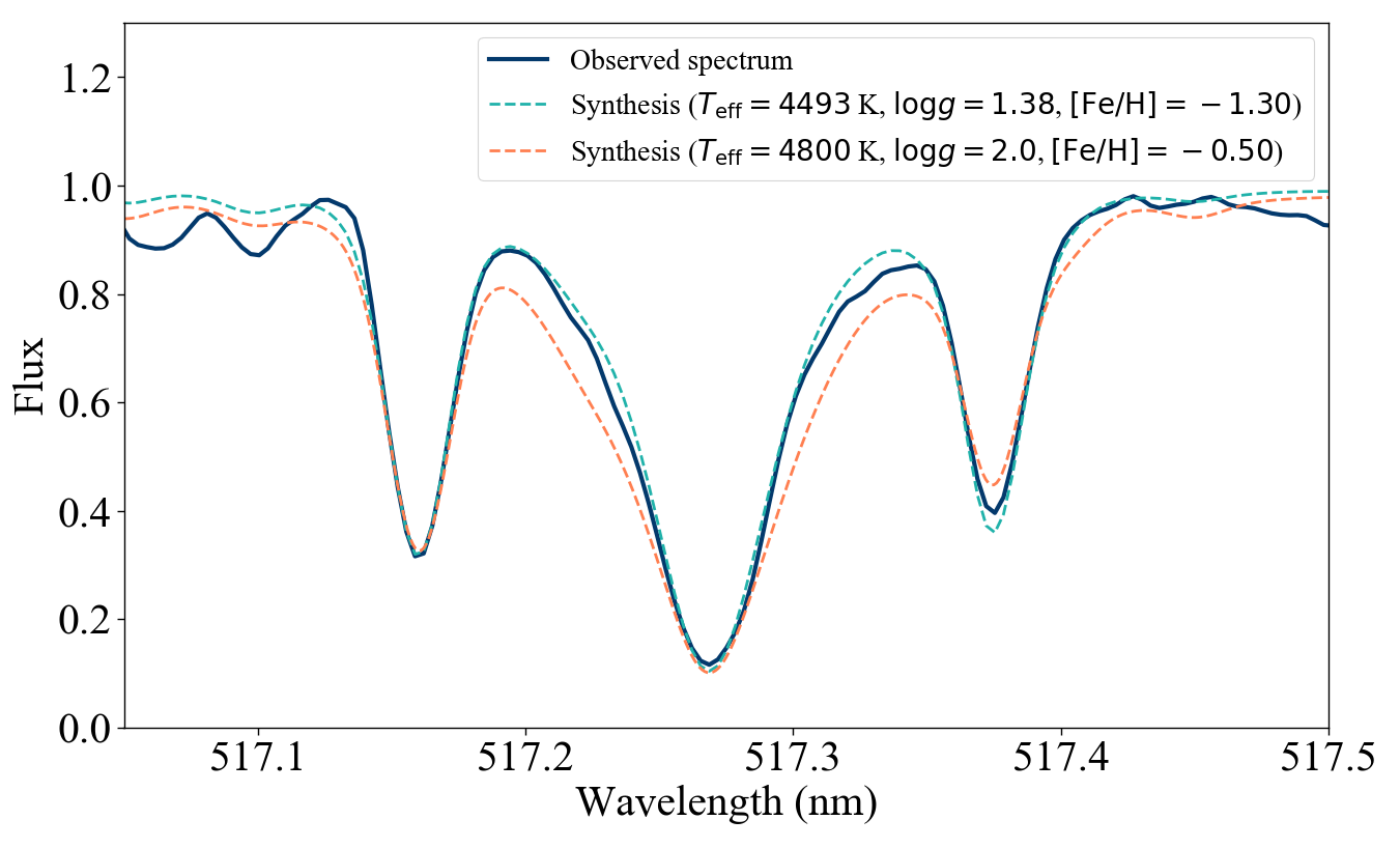
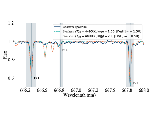
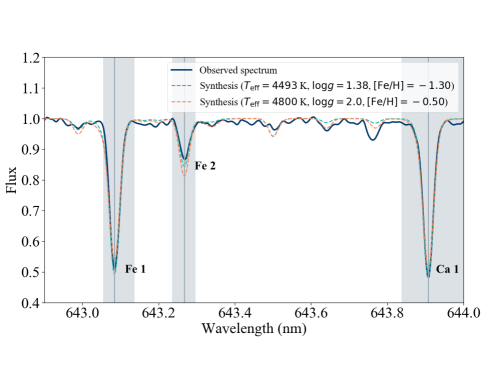
In order to determine atmospheric parameters we adopted a similar procedure as the one implemented in Casamiquela et al. (2019). We considered the line list from the Gaia-ESO survey (Heiter et al., 2015a), which includes atoms and molecules, and the Grevesse solar abundances (Grevesse et al., 2007). Within iSpec we chose the 1D atmospheric models MARCS7 (Gustafsson et al., 2008) and the LTE radiative transfer code TURBOSPECTRUM (Alvarez & Plez, 1997; Plez, 2012). We considered in our analysis only the region between 480 nm and 660 nm, since bluer regions have lower signal to noise and also because iSpec has been largely tested in the adopted region. When iSpec uses TURBOSPECTRUM, it considers the technique of fitting synthetic spectra to the observations, in specific regions defined by the user, in this case those listed in Table 3 in the Appendix A. The atmospheric parameters are with this method determined by fitting on-the-fly the selection of spectral regions simultaneously until a good match between the synthesis and the observation is achieved (following a $\chi^{2}$ minimisation procedure). After the atmospheric parameters are decided, the chemical abundances can be determined line-by-line, using syntheses with the same radiative transfer code. The lines used to derive chemical abundances are also found in the Appendix A, in Table 4. After generating the synthetic spectra, we visually verified the good agreement between it and the observed spectra. In Figure 2, we show a comparison between the synthetic spectrum built with our best fit stellar parameters (green dashed lines) and the observed spectrum (solid blue lines). We also show the synthetic spectrum built using the stellar parameters from Massey et al. (2018) (dashed orange lines). There is a good agreement between the observed spectrum and the synthetic one based on our best fit stellar parameters in the gray regions, which are those used for performing the fitting. The regions chosen to display the agreement between synthesis and observations focus on the Mg triplet at 517 nm, and other regions in which both neutral and ionised iron lines of different strengths and excitation potentials fall. We note that the synthetic spectrum built using the stellar parameters presented in this work agree better with the observed one than the synthetic spectrum built using stellar parameters from the literature. Only the regions of Fe 1 and Fe 2 were considered for the determination of parameters, relying on the method of ionisation and excitation balance (Gray, 2005): effective temperature does not need to depend on the strength or excitation potential of Fe 1 lines, and the metallicity needs to give the same result for Fe 1 and Fe 2 lines. This is achieved by adjusting the value of surface gravity, which depends on the strength of Fe 2 lines. The Mg triplet, which in this case was not used for the fitting, is displayed here as diagnostics, since its wings are very dependent on surface gravity. The good agreement between the synthetic spectrum based on our parameters and the observed spectrum in these regions indicates that $T_{\mathrm{eff}}$, $\log g$ and [Fe/H] are consistently calculated, addressing possible degeneracies in the parameters. In our analysis we did not include H lines because they suffer from strong non-LTE and 3D effects (Amarsi et al., 2018), but in Appendix B we give further discussions on the H line profiles for completeness.

Figure 2: Comparison between observed spectra (solid blue lines) and synthetic spectra (dashed green lines) based on our best fit stellar parameters. Dashed orange lines show the synthetic spectra built using stellar parameters from the literature. Top panel: region containing the magnesium triplet. Middle panel: region containing Fe 1 lines. Bottom panel: region containing Fe 1, Fe 2 and Ca 1 lines. The gray regions indicate the area of the different lines used as an example. The synthesis based on our best fit stellar parameters considers a star of $T_{\mathrm{eff}}=4493$ K, $\log g=1.38$ and $\mathrm{[Fe/H]}=-1.30$. The synthesis based on literature stellar parameters considers $T_{\mathrm{eff}}=4800$ K, $\log g=2.0$ and $\mathrm{[Fe/H]}=-0.5$.

With the aim of validating our atmospheric parameters, we considered a control sample of metal-poor stars studied by Car21 and for which we have parameters from the APOGEE survey. In this case, we used APOGEE $T_{\mathrm{eff}}$, $\log g$ and [Fe/H] as reference values, testing the accuracy of our data as well as estimating external uncertainties. We chose not to compare our stellar parameters with the ones presented in Car21, because the analysis done in that work is not fully spectroscopic.

Figure 3: Comparisons of our atmospheric parameters with APOGEE. Top panel: difference in effective temperature. Central panel: Difference in surface gravity. Bottom panel: difference in metallicity. The mean $\mu$ as well as the standard deviation $\sigma$ of each distribution is included in the panels. The uncertainties are computed as the quadratic sum of uncertainties from the pipeline and from the literature value.

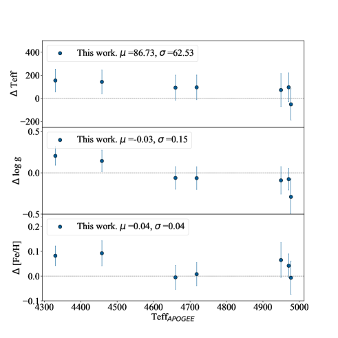
In Figure 3 we compare our results for the control sample. We plot the difference between the atmospheric parameters T_eff, $\log g$ and [Fe/H] obtained in our work and values from APOGEE survey. The mean of the differences between the results and the standard deviation are indicated in each panel for reference.

For all stars, there is a consistency between T_eff obtained by us and T_eff from APOGEE within 1 sigma. Nevertheless, we observe that our T_eff tend to be higher than the APOGEE results by $87\pm 63$ K. In regard to $\log g$, all values obtained in this work agree with APOGEE values within 2 sigma. The mean difference of log g is -0.03 and the standard deviation is 0.15. Regarding the metallicity, there is an agreement within 2.2 sigma when comparing measured values from our work and APOGEE values. The mean difference for the metallicity is 0.04 dex, the standard deviation is 0.04 dex, thus there is a slight offset in which we obtain metal-richer results than APOGEE.

We obtained $T_{\mathrm{eff}}=4493\pm 102$ K, $\log g=1.38\pm 0.15$ and $\mathrm{[Fe/H]}=-1.30\pm 0.1$ for J01020100-7122208. Here we considered as the uncertainty of our measurements the quadratic sum of the internal value provided from our pipeline and the standard deviation from the comparison presented in Figure 3. Our parameters point towards the star being a metal-poor red giant star, even when considering the systematic offset obtained with respect to APOGEE, which agrees with Mas18 but not with Neu18. In any case, our study indicates that the star is more metal-poor then previously reported, and is consistent with the star being a member of the stellar halo.

3.2 Kinematics

We calculated the velocities $(U,V,W)$ for J01020100-7122208 using the astropy package (Robitaille et al., 2013; Price-Whelan et al., 2018). We adopted a Galactic height of $z_{\odot}=0.0025$ Kpc (Jurić et al., 2008) and Galactic radius $R_{\odot}=8.2$ Kpc (McMillan, 2016) for the Solar position, and $(U,V,W)_{\odot}=(11.10,247.97,7.25)$ km s^-1 for the Solar velocity relative to the Galactic Center, following Matsuno et al. (2020). We used right ascension, declination and proper motions from Gaia EDR3 and the RVs obtained from our MIKE spectra. We adopted $U$ positive toward Galactic Center, $V$ positive in the direction of Galactic rotation and $W$ positive toward the North Galactic Pole. The final velocity in the Galactic rest frame is $(U,V,W)=(-185.26,-171.64,-159.30)$ km s^-1. This indicates that the star is counter-rotating, e.g. it is part of the retrograde halo, which is consistent with the metal-poor nature of the star.

3.3 Distance and other stellar properties

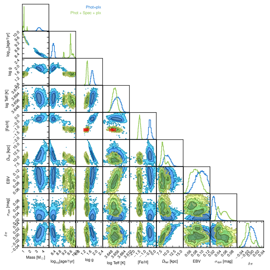
We use the minimint package (Koposov, 2020) that relies on the MIST library of synthetic isochrones (Dotter, 2016; Choi et al., 2016) to map the mass, age and metallicity to absolute magnitudes in a variety of filters as well as surface gravity and effective temperature. We then model the observed photometry, Gaia parallaxes, and spectroscopic stellar atmospheric parameters similarly to Koposov et al. (2020). The model parameters are the mass, age, metallicity, extinction, distance to the star and an additional systematic photometric scatter that is added in quadrature to all the magnitude uncertainties. We use the optical photometry from Gaia EDR3 (Riello et al., 2021) and Skymapper DR2 (Onken et al., 2019) and IR photometry from 2MASS (Skrutskie et al., 2006) and WISE surveys (Eisenhardt et al., 2020). As the parallax solution of Gaia is known to have systematic spatially dependent biases (Lindegren et al., 2021) we also introduce an additional parallax offset parameter with a $\delta\omega/(1{\rm mas})\sim N(0,0.02)$ prior. We use the Nested Sampling algorithm MULTINEST (Feroz & Hobson, 2008) as implemented in Python by Buchner et al. (2014) to sample the posterior. Similarly to Koposov et al. (2020) we run the model in two configurations, one where the photometry alone is modeled, and a second where we use the stellar atmospheric parameters in the fit together with photometry.

Table 2: Result of Spectrophotometric Analysis

Property	Photometric	Spectrophotometric
Mass ($M_{\odot}$)	$3.39\pm 0.25$	$1.09\pm 0.10$
Age ($\mathrm{Gyr}$)	$0.244\pm 0.041$	$4.507\pm 1.437$
Distance ($\mathrm{kpc}$)	$10.39\pm 1.17$	$8.74\pm 0.74$
Extinction ($\mathrm{mag}$)	$0.102\pm 0.017$	$0.083\pm 0.016$
Systematic error ($\mathrm{mag}$)	$0.028\pm 0.007$	$0.053\pm 0.015$
Parallax offset ($\mathrm{mas}$)	$0.0034\pm 0.0122$	$-0.0092\pm 0.0146$

We show the posterior of our photometric and spectrophotometric analyses in Fig. 4 and the corresponding means and standard deviations of the posterior samples in Table 2. These two analyses are in some tension, with the photometric analysis favouring an interpretation of the star as a young, metal-rich, high-mass giant star while the spectrophotometric analysis favours it to be an old, metal-poor, low-mass giant star. We note that the photometric-only analysis implies values of $T_{\mathrm{eff}}$, $\log g$ and $[\mathrm{Fe}/\mathrm{H}]$ which are entirely inconsistent with the values we measured from the spectra.

We note that the results of photometric data only are closer to those of Massey et al. (2018). Considering that in that case both analyses use Gaia data and were based on the same technique, this is expected. Our high resolution analysis however points towards a star that is significantly more metal-poor than previously believed. It is well-known that metalliticies can have a large impact on stellar models (Tayar et al., 2017, e.g.), causing a large systematic effect if solar-metallicities are considered for metal-poor stars. We see here how a high resolution spectrum can provide additional useful information. Furthermore, in Appendix B we verified from the hydrogen lines that our spectroscopic results are consistent with those line profiles (what was also illustrated in Figure 2), hence confirming that a spectrophotometric analysis in this case is needed.

Therefore, our discussion will assume that this star is indeed an old, metal-poor, low-mass giant star, since it is the result obtained when we use more complete information about J01020100-7122208.

Figure 4: Corner plot of the posterior from our photometric (blue) and spectrophotometric (green) analyses of the star. The red point is the measurement of the atmospheric properties derived from the spectrum.

3.4 Orbit calculation

We characterised the full variety of possible orbits of this star through the Galaxy by drawing random values from our posterior on the present day distance, proper motion and radial velocity and integrating them forwards and backwards in time. The spectrophotometric analysis above yields a posterior on the distance to the star and we can sample the radial velocity from the normal distribution given by our measured mean and uncertainty. However, more work was needed to obtain samples of the proper motions.

The spectrophotometric analysis of the previous section yields a posterior on the distance to the star which is both more precise and shifted relative to the parallax reported by Gaia. The uncertainty in Gaia’s measurement of a star’s parallax is correlated with the uncertainty in the proper motion, meaning that any extra information on a star’s true parallax will also cause our estimate of the star’s proper motion to change. The implication of this is that randomly sampling the proper motions from the Gaia reported means and uncertainties will yield proper motions which are inconsistent with our best estimate of the distance.

Gaia describes the correlation between the parallax and proper motions through a trivariate normal distribution with mean $\boldsymbol{m}=(m_{\varpi},m_{\mu\alpha\ast},m_{\mu\delta})^{\intercal}$ and covariance matrix $\mathbf{S}$. The spectrophotometric posterior on the distance cannot in general be described as a normal distribution, so we instead treated each posterior sample as giving a point estimate of the true parallax $\tilde{\varpi}$. We then conditioned the proper motion distribution on each of those values in turn to derive updated estimates of the mean $\tilde{\bf{m}}_{\mu}$ and covariance matrix $\tilde{\mathbf{S}}_{\mu\mu}$ of the bivariate normal distribution on the proper motions, through the equations

$$\tilde{\boldsymbol{m}}_{\mu}=\boldsymbol{m}_{\mu}+\frac{\tilde{\varpi}-m_{\varpi}}{\sigma_{\varpi}^{2}}\mathbf{S}_{\mu\varpi},$$ (1)

$$\tilde{\mathbf{S}}_{\mu\mu}=\mathbf{S}_{\mu\mu}-\frac{1}{\sigma_{\varpi}^{2}}\mathbf{S}_{\mu\varpi}\mathbf{S}_{\varpi\mu},$$ (2)

where quantities like $\mathbf{S}_{ab}$ refer to the corresponding submatrices. We drew one sample from each of these distributions, such that for each distance sample from the spectophotometric posterior we had a consistent proper motion sample.

For 2,500 of these samples, we integrated the orbit of the star forward and backward in time for $1\;\mathrm{Gyr}$ using the gala (Price-Whelan, 2017) Python package, assuming the default Milky Way potential and transforming into the Galactocentric coordinate frame using the latest astropy recommended values (Reid & Brunthaler, 2004; Gravity Collaboration et al., 2018; Drimmel & Poggio, 2018; Bennett & Bovy, 2019).

Figure 5: A random sample of 250 possible past and future trajectories of the star through the Galactic potential. The location of the Sun is marked with a yellow star, the Galactic centre with a cross and the Milky Way disk with a dashed ellipse.

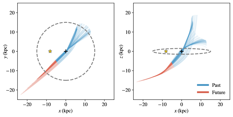
We show in Fig. 5 a random subsample of 250 orbits out of the 10,000 orbits that we integrated. While the uncertainty in the present day distance to the star (in particular the second mode visible in Fig. 4) produces a spread of trajectories, the main bulk of the trajectories pass close to the centre of our Galaxy. To test the hypothesis that this star originates in the Galactic centre, we identified where each past trajectory last crossed the Galactic disk, finding that the star last crossed the plane at a distance of $550_{-361}^{+1129}\;\mathrm{pc}$ from the Galactic centre and that the crossing location was at least $113\;\mathrm{pc}$ from the Galactic centre with 99 per cent confidence. Another way of expressing this is that the star’s eccentricity is $0.917_{-0.025}^{+0.005}$, making this star’s orbit highly eccentric but not perfectly radial. If we repeat the orbit integration with the photometric analysis, then we find that the star last crossed the plane at a distance of $2673_{-1721}^{+2329}\;\mathrm{pc}$ from the Galactic centre and that the crossing location was at least $135\;\mathrm{pc}$ from the Galactic centre with 99 per cent confidence. Neither of the analyses support the hypothesis that the star originated in the Galactic centre.

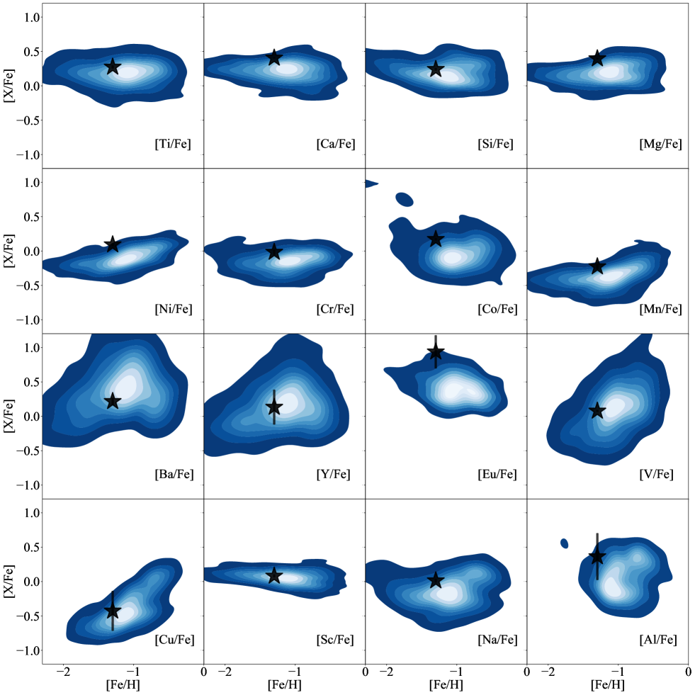
4 Chemical abundances

The chemical abundances can be seen in Figure 6, where we show J01020100-7122208 as a black filled star. In each panel we display the measured abundance ratio [X/Fe] of a different element. In the same figure, we adopted as reference a sample of retrograde stars from the GALAH survey (Buder et al., 2020), represented as contours of a kernel density estimation. The control sample was taken from the DR3 of GALAH, selecting only stars with T_eff $\leq$ 5500 K and $\log g$ $\leq$ 2.0. We also did a quality selection, where we chose only stars with flag_sp = 0 (i.e. no problems with the determination of parameters), flag_fe_h = 0 (i.e. no problems in the determination of [Fe/H]) and flag_X_fe = 0 (no problems in the determination of the abundance [X/Fe]). Further details can be found in Buder et al. (2020).

For all these stars we used Gaia positions, proper motions and RVs to calculate the respective total velocities. We selected only stars with $V\leq 0$ km s^-1. Since J01020100-7122208 is a retrograde star, we compared its chemical composition with other stars to see if they come from the same Galactic component. In general we find that the chemical composition of J01020100-7122208 is very similar to the GALAH retrograde stars. The results of individual chemical elements is discussed in more detail below.

Figure 6: Chemical abundances. Black star refers to J01020100-7122208. Blue contours refer to a kernel density estimation of retrograde stars from GALAH survey used here as a reference sample.

4.1 $\alpha$ elements

$\alpha$ elements are those formed by the capture of $\alpha$ particles in the core of stars during post-main sequence burning and are dispersed in the interstellar medium (ISM) mainly by core collapse Type II supernovae (SNII) (e.g. Timmes et al. 1995, Kobayashi et al. 2006, Nomoto et al. 2013). In this work we explore the following $\alpha$ elements: calcium (Ca), silicon (Si) and magnesium (Mg). We also explore titanium (Ti), that according to nucleosynthetic models is not produced by the $\alpha$-capture channel but the [Ti/Fe] distribution as a function of [Fe/H] behaves like other $\alpha$ elements.

Following the time-delay model (Tinsley, 1979; Matteucci & Greggio, 1986), there is a delay in the ejection of Fe-peak elements such as Fe and Mn by Type Ia supernovae (SNIa) when we compare it with the fast ejection of $\alpha$ elements by SNII. The result of the time-delay enrichment of Fe, for example, is that the oldest stars are both $\alpha$-rich and metal-poor. This class of elements are also an indicator of the star formation rate of a progenitor galaxy: the richer a star is in $\alpha$-elements, the higher the star formation rate of the progenitor galaxy (Gilmore & Wyse, 1998).

The top row of Figure 6 shows the abundance ratios of $\alpha-$elements and it is possible to see that J01020100-7122208 is an $\alpha$-rich star ([$\alpha$/Fe] $\approx$ 0.30). This enhancement is consistent with the star being old. It is further seen that J01020100-7122208’s [$\alpha/$Fe] has abundance ratios consistent with the retrograde GALAH stars.

4.2 Iron-peak elements

Iron-peak elements are formed by several different nucleosynthetic channels, but are mainly dispersed into the ISM by SNIa (Iwamoto et al., 1999), in the same way as iron. In this work we explored four iron-peak elements: nickel (Ni), cobalt (Co), chromium (Cr) and manganese (Mn) seen in second row of Figure 6. Cr is a chemical element that follows the behaviour of iron, which is seen in Figure 6, where the abundance of this element is similar for all stars. On the other hand, Mn varies with the metallicity and is a good trait to distinguish populations. Mn for example is a very good tracer of SNIa because it is more produced in SNIa than SNII in relation to Fe (Kobayashi & Nomoto, 2009).

In Figure 6, we see that the star is in the Mn-rich part of the diagram, indicating that among the retrograde halo population stars, it is likely not part of the oldest stars of this component. In the same figure, we can see that Co does not vary with the metallicity, while Ni shows a slight increase with the metallicity. Also, from the control sample we can see that there is a Ni-rich population of stars in this Galactic component, but J01020100-7122208 is not part of this sub-population.

4.3 Neutron-capture elements

Neutron capture elements can be divided in two subclasses: the r-process elements and the s-process elements. In this work we studied the s-process elements yttrium (Y) and barium (Ba) as well as the r-process element europium (Eu). S-process elements are produced by low- to intermediate-mass AGB stars (Busso et al., 1999), while Eu is believed to be produced mostly in neutron star mergers (Matteucci et al., 2014). The abundances of Y and Ba measured in J01020100-7122208 agree well with our control sample. J01020100-7122208 shows an overabundance of europium (Eu), having a measured value of 0.93 $\pm$ 0.24. Both Matsuno et al. (2021) and Aguado et al. (2021) reported that accreted stars from a progenitor galaxy named Gaia-Enceladus (Belokurov et al., 2018; Helmi et al., 2018) shows an overabundance of this element, with a central distribution of [Eu/Fe] $\approx$ 0.5, but also containing stars with higher abundances. The overabundance of [Eu/Fe] is evidence that J01020100-7122208 may be an accreted star from Gaia-Enceladus.

Figure 7: Spectrum of J01020100-7122208 near the region of the lithium line at 670.7 nm. The vertical yellow line and region represents where the Li line should be if observed.

4.4 Odd-Z elements

In this work we measured chemical abundances of five odd-Z elements: sodium (Na), aluminum (Al), copper (Cu), vanadium (V) and scandium (Sc). Na and Al are thought to be produced by SNII, having a production dependent on the abundance of C and N in the environment (Kobayashi et al., 2006) as well as with the metallicity of the progenitor (e.g. Das et al. 2020).

They are also believed to be produced by AGB stars (Nomoto et al., 2013). From Figure 6, we can see that the abundances of these two chemical elements agree well with the chemical abundances of retrograde halo stars. While Cu is thought to be formed through different channels including week s-process, SNIa, hypernovae and by massive stars (Pignatari et al., 2010; Nomoto et al., 2013), V is through to be produced mainly in explosive silicon burning in SNII and Sc is believed to be produced in carbon and neon burning phases in massive stars (Woosley & Weaver, 1995). In Figure 6 we can see that the abundances of these three elements are compatible with the typical abundance of retrograde halo stars.

4.5 The absence of lithium

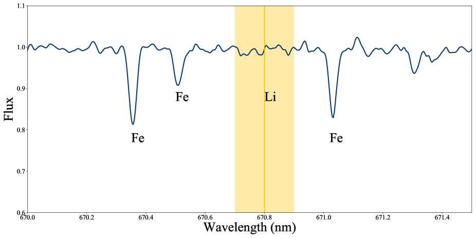
Lithium (Li) is a chemical element that can correlate with the age of stars (Randich & Magrini, 2021, and references therein). Li is burned very fast in stars and the intensity of depletion is related with the mass of the star, with the main depletion process occurring even before the main sequence. The depletion of Li in massive stars is not relevant, but it is very important in low-mass stars, independent of the metallicity. Therefore, regular metal-poor red giants stars do not show the presence of Li. From our spectrum, we could not detect Li, which is further evidence of the hypothesis that this star is a regular old red giant. We present in Figure 7 the spectrum of J01020100-7122208 in the region near the lithium line at 670.7 nm. The position of the line is indicated in yellow and shows no line.

5 The origin and nature of J01020100-7122208

In contrast to what was reported by Neu18 and Mas18, here we find that J01020100-7122208 is a low-mass (1.09 $\pm$ 0.10 M$\odot$) intermediate-age (4.51 $\pm$ 1.44 Gyr) metal-poor ([Fe/H] = -1.30 $\pm$ 0.10) red giant star. Both Neu18 and Mas18 concluded this star was young. Neu18 determined an age of 30 Myr, while Mas18 obtained an age of 180 Myr. This is a consequence of the rather high masses determined in these works, of 9 and 3-4 M$\odot$, respectively.

The main conclusion of Mas18 was that this star was likely an object accelerated by the central black hole of the Milky way. Here, with improved astrometric data from Gaia EDR3 combined with a detailed high resolution spectral analysis, we found instead that the star probably passed about 550 pc away from the central black hole, which is too far for it to have been ejected from the centre.

Furthermore, Mas18 reported a metallicity of [Fe/H] = -0.5, while we obtained a value of [Fe/H] = -1.30 $\pm$ 0.10. In Mas18, their metallicity and age led them to conclude that this star originated in the Milky Way disk. In our work, we found that the star has a retrograde velocity, which, together with its low metallicity and high [$\alpha$/Fe] ratio, make it likely to belong to the halo. Here, however, our age is not the typical age of halo stars (of approximately 10 Gyr, Jofre & Weiss, 2011; Kalirai, 2012; Das et al., 2020). Further discussions are found below.

5.1 Chemistry

From the atmosphere of low-mass stars it is possible to measure chemical abundances that imprint the chemical composition of the molecular cloud from which the star was born. This is assuming that stellar internal processes do not significantly impact the chemical elements in the surface of the star. Therefore, by examining the chemical composition of this star, we can shed light about its origin. We considered $\alpha-$ elements (Ca, Si, Mg and Ti), iron-peak elements (Ni, Cr, Co and Mn), odd-Z elements (Na, Al, Cu, V, Sc) and neutron-capture elements (Y, Ba and Eu).

From Figure 6 it was possible to see that the chemical abundances of J01020100-7122208 agree well with the distribution of retrograde stars, which corroborates the hypothesis that this star, although fast, is a member of this component. It is believed that the Milky Way retrograde halo is partially formed by stars accreted from other galaxies (Gratton et al., 2003; Carollo et al., 2007). Therefore, J01020100-7122208 might be one such star that was formed in another galaxy and was accreted later into the Galaxy.

As mentioned before, $\alpha-$elements are good tracers of star formation rate. A star with enhanced values of [$\alpha$/Fe] is evidence that it was born in an environment were the star formation rate was high. In the case of low-mass dwarf galaxies, we have an environment where the star formation rate is lower than in the Milky Way (Tolstoy et al., 2009; Nissen & Schuster, 2010). Therefore, it is expected that stars born there are more $\alpha$-poor than stars born in situ (Nissen & Schuster, 2010). But if the progenitor galaxy was relatively massive (of the order of $10^{9-10}$ M_⊙), the values of $\alpha$ elements in the low metallicity regime can be similar to the one observed in metal-poor stars of the Milky Way (Das et al., 2020). J01020100-7122208 is a star of high [$\alpha$/Fe] abundance ratios compared to the rest of the counter-rotating halo stars from GALAH (see Fig. 6). Thus, if accreted, the progenitor galaxy should have been massive. In particular, it is possible that the progenitor was Gaia-Enceladus (Belokurov et al., 2018; Helmi et al., 2018), with a mass of $\approx$ 10⁹ M_⊙ (Vincenzo et al., 2019; Das et al., 2020; Feuillet et al., 2020). We also note that chemical abundances of J01020100-7122208 agree well with the chemical pattern of Gaia-Enceladus stars analysed by Matsuno et al. 2019, and Car21.

5.2 Age

The high $\alpha$ abundance together with the low metallicity are strong evidence that this star is old (Schuster et al., 2012; Hawkins et al., 2014; Montalbán et al., 2021). The fact that the star has a low abundance of Mn reinforces this suggestion. This star however is not as old as other regular halo stars.

Chiappini et al. (2015) reported few CoRoT (Baglin et al., 2006) red-giant stars that despite being metal-poor and enhanced in [$\alpha$/Fe], are apparently young (younger than 7 Gyr approximately). In that work, the authors proposed that they formed near the bar co-rotation, which is a region where gas can be kept inert for longer times than in other places of the Galaxy (Bissantz et al., 2003; Combes, 2013). These young $\alpha$-rich (Y$\alpha$R) stars were also reported in Martig et al. (2015), where the authors found 14 of these objects in Kepler (Borucki et al., 2010), where 5 of them had ages below 4 Gyr.

Currently, there are two main explanations for the Y$\alpha$R stars, though neither are fully conclusive. The first scenario, mentioned above (Chiappini et al., 2015; Zhang et al., 2021) is that the stars are truly young and have originated near the Galactic center and migrated outwards. The other scenario (Jofré et al., 2016; Yong et al., 2016) postulates that these stars were binary stars which experienced mass transfer, e.g. they are evolved blue stragglers. Hence, the ages were probably not calculated correctly and these stars are not really younger than typical old stars. The challenge is that not all such stars show evidence of binary evolution (Silva Aguirre et al., 2018; Hekker & Johnson, 2019). Given that the elemental abundances and kinematics of such stars mimics those of old stars (Matsuno et al., 2018), it is very difficult to explain their origins being different than normal thick disk or halo stars. On the other hand, considering the poor evidence of variation in RV and no obvious high rotation from the line profiles (Jofré et al., 2016; Silva Aguirre et al., 2018) it is not necessary that J01020100-7122208 is in a binary system now. However, the binary could have merged (Izzard et al., 2018).

It is also possible that the star was part of a binary system in the past and when the companion exploded, J01020100-7122208 was ejected with higher velocity. That scenario was proposed by Neu18 and Mas18. In both cases, the star might have been ‘rejuvenated’ like a blue straggler, explaining our age determination of 4 Gyr.

As discussed in Martig et al. (2015) neither the uncertainties of the measured ages or the uncertainty related to their methodology are big enough to explain the young ages. Similarly, considering the uncertainty of the age measured in our work, we can not claim this star is as old as typical retrograde halo stars. In general, age determination is a challenging task. In the case of seismic ages (such as the ones reported in Chiappini et al. 2015 and Martig et al. 2015), to calculate accurate ages of metal-poor giants is challenging because corrections are required in the scaling relations when studying metal-poor stars (Epstein et al., 2014) and also because since mass loss is not a very well known process, in the case of stars in the red clump, the mass loss experience is previous evolutionary phases can not be well accounted for (see Anders et al. 2017; Montalbán et al. 2021). In the same way, calculating ages of metal-poor giant stars using isochrone-fitting techniques (as done in this work) is also challenging since the isochrones tend to clump together in the region of the red giant branch (as commented in Martig et al. 2015).

5.3 Kinematics

We found that the star last crossed the Galactic plane at least $113\;\mathrm{pc}$ from the Galactic centre with 99% confidence, arguing against acceleration by Sgr A^∗. We note that we have not included the uncertainties in the Galactic potential or the Solar position and motion when calculating that confidence interval, and that it may be more plausible for this star’s orbit to have passed through the Galactic centre if those are included. However, the null hypothesis must be that this star is an eccentric halo star, since the eccentricity, angular momentum and energy are fully consistent with that hypothesis.

A useful contrast can be found with the only star known to have been accelerated by Sgr A^∗, S5-HVS1. Koposov et al. (2020) followed a near-identical procedure to this work and found that the 90% confidence region of the star’s last crossing through the Galactic plane included the Galactic centre. However, the strongest evidence of the Galactic centre hypothesis was S5-HVS1’s young age (less than $100\;\mathrm{Myr}$) and extreme velocity ($1755\;\mathrm{km}\;\mathrm{s}^{-1}$), which ruled out any other hypothesis. The star J1020100-7122208 is unlikely to have crossed the plane near the Galactic centre and is old and slow-moving, with a current velocity of $257\pm 23\;\mathrm{km}\;\mathrm{s}^{-1}$. An extreme scenario is not required to explain its kinematics.

5.4 Putting the puzzle together

From the abundances alone, we conclude that if the star is an accreted object, the progenitor must have been relatively massive. In particular, it is possible that the progenitor is Gaia-Enceladus, since the chemical pattern of J01020100-7122208 is in good agreement with what was reported by Matsuno et al. 2019, and Car21 for stars from this progenitor. Another evidence that chemically supports the idea that the progenitor is Gaia-Enceladus is the overabundance of [Eu/Fe]. Based on the Toomre diagram presented in Koppelman et al. (2019) that shows the velocity distribution of stars from different progenitors including Gaia-Enceladus, and other dwarf galaxies like Sequoia, Thamnos 1 and Thamnos 2, we see that J01020100-7122208 has a velocity profile consistent with Sequoia stars having $V=-171.64$ km s^-1 and $\sqrt{U^{2}+W^{2}}=244.33$ km s^-1. However, J01020100-7122208 has a highly eccentric orbit (with an eccentricity of about 0.9). Koppelman et al. (2020) reported that 75 per cent of Gaia-Enceladus stars have eccentricities higher than 0.8 (see also Mackereth et al. 2018), while Myeong et al. (2019) reported that the typical eccentricity for Sequoia stars is 0.6. It is possible that the star comes from Gaia-Enceladus or Sequoia, although the chemistry is more consistent with Gaia-Enceladus. In any case, its origin is most likely extragalactic and therefore its younger age suggests it is rather an evolved blue straggler and not a younger star coming from the inner Galaxy. Y$\alpha$R stars there were likely accreted by the Milky Way have been reported before in the literature (e.g. Das et al. 2020).

6 Conclusion

J01020100-7122208 is a star which was reported as a serendipitous discovery a decade ago. Before the Gaia survey, this star was claimed to be a runaway yellow super giant from the Small Magellanic Cloud (Neugent et al., 2018). Immediately after Gaia Data Release 2, the star was reanalysed and claimed to be likely formed in the Milky Way disk and ejected to the halo by the central black hole of the Galaxy (Massey et al., 2018). This latter work warned that with newer Gaia data releases this conclusion could change. Therefore, now that Gaia EDR3 is available, the time is right to revisit this mysterious object.

In our work, we analysed J01020100-7122208 using astrometric, photometric and spectroscopic data to determine its age, orbit and chemical composition. It is the first time this star was chemically characterised. From our analysis we found that this star is a metal-poor red giant, with a metallicity of [Fe/H] = -1.30 $\pm$ 0.10. This metallicity value is lower than previously reported: Massey et al. (2018) obtained a metallicity of [Fe/H] = -0.5. We also found that this star is a retrograde halo star with a very high eccentricity of $0.917_{-0.025}^{+0.005}$. We obtained an age of $4.51\pm 1.44$ Gyr, and a mass of $1.09\pm 0.10$ $M_{\odot}$. We also found that the star likely last passed $550\;\mathrm{pc}$ away from the Galactic centre. This does not support the idea that the star was ejected from the supermassive black hole at the centre of the Galaxy.

In terms of chemical abundances, the star has a chemical pattern compatible with typical retrograde stars, supporting the idea that the star is part of the retrograde halo. We also found that the low metallicity, combined with the high abundance of $\alpha$ elements, is an indicator that the star is old and formed in an environment with a high star formation rate. Considering that the star is part of the retrograde halo, it is possible that it was born in another galaxy and later accreted onto the Milky Way. We found an overabundance of europium of [Eu/Fe] = 0.93 $\pm$ 0.24, indicating that J01020100-7122208 might come from the Gaia-Enceladus galaxy.

Our age of 4 Gyr is slightly inconsistent with our results from the chemistry, which points towards a star formed before 4 Gyr ago. We attribute this inconsistency to the difficulties regarding the age determination of metal-poor red giant stars and also to the idea that this star could be the product of a merge between two stars, rejuvenating the star like a blue straggler.

Based on the kinematics, ages and chemical abundances of 16 elements, we concluded that this star is not likely to have been ejected from the central black hole of our Galaxy, but instead is an accreted star, probably from Gaia-Enceladus. To arrive at this conclusion, it was necessary to combine astrometric, photometric and spectroscopic information. We have demonstrated that to truly understand where a star comes from, the best is to combine information about kinematics, ages and chemical abundances. With kinematics we can retrieve the trajectory a star has followed. With ages we can both constrain the orbits of stars and associate an object to a stellar population. With chemical abundances we can both validate possible origins retrieved from kinematics and also point out new origins. We are entering a revolutionary time in Galactic archaeology in which we have all this information for millions of stars.

Data Availability

The data underlying this article will be shared on reasonable request to the corresponding author. The GALAH DR3 data used in this work can found at https://www.galah-survey.org/dr3/the_catalogues/. The GAIA EDR3 data used in this work can be found at https://www.cosmos.esa.int/web/gaia/earlydr3.

Appendix A Adopted line regions

In order to calculate the stellar parameters of J01020100-7122208, we used a list of lines adjusted on the list synthe_synth_good_for_params, which is provided with the package of iSpec. This list was built using as a basis the Gaia-ESO linelist.

With the aim of having a better agreement between the values of stellar parameters calculated for our control sample and the reference values provided by APOGEE survey, we considered regions sensitive to stellar parameters, in particular those with Fe 2 lines that help with the calculation of the surface gravity. In Table 3, we present the lines used when calculating stellar parameters. The lines used to calculate chemical abundances are presented in Table 4.

Table 3: Lines used to calculate stellar parameters of J01020100-7122208.

Wavelength	Element	Wavelength	Element	Wavelength	Element	Wavelength	Element	Wavelength	Element	Wavelength	Element
482.4127	Cr 2	507.9740	Fe 1	531.2856	Cr 1	550.6779	Fe 1	583.8372	Fe 1	624.0310	Fe 1
482.0417	Zr 2	508.3338	Fe 1	531.7525	Fe 1	551.2257	Fe 1	584.6993	Ni 1	624.0646	Fe 1
482.9373	Cr 1	508.4096	Ni 1	531.8771	Cr 1	551.4435	Cr 1	585.2293	Fe 2	624.3815	Si 1
483.8556	Fe 2	508.7058	Ti 1	531.9035	Fe 1	554.6990	Fe 1	585.5076	Fe 1	624.6318	Fe 1
488.1591	Mn 1	509.0773	Fe 1	532.0036	Fe 1	554.9949	Fe 1	585.7752	Ni 1	625.2555	Fe 1
491.5229	Ti 1	509.9930	Ni 1	532.2021	Fe 1	556.5541	Fe 2	585.8778	Fe 1	625.9595	Ni 1
491.8012	Fe 1	510.4030	Fe 1	532.5552	Fe 2	556.7351	Fe 1	585.9586	Fe 1	626.5132	Fe 1
491.8994	Fe 1	511.0413	Fe 1	532.6161	Fe 1	556.9618	Fe 1	586.1109	Fe 1	627.1278	Fe 1
491.9861	Ti 1	511.5392	Ni 1	532.7252	Fe 1	557.2842	Fe 1	586.7562	Ca 1	630.1500	Fe 1
492.0502	Fe 1	512.0415	Ti 1	532.9784	Cr 1	557.3102	Fe 1	587.7788	Fe 1	630.2493	Fe 1
493.6335	Cr 1	512.4619	Fe 1	532.9989	Fe 1	557.6089	Fe 1	589.9292	Ti 1	631.5306	Fe 1
493.7348	Ni 1	512.5117	Fe 1	533.1481	Fe 2	558.6756	Fe 1	590.2473	Fe 1	631.5811	Fe 1
493.8254	Ti 1	512.7359	Fe 1	533.2900	Fe 1	558.8749	Ca 1	590.3319	Fe 2	631.8018	Fe 1
493.8814	Fe 1	513.0359	Ni 1	533.6786	Ti 2	561.4773	Ni 1	591.0003	Fe 2	632.2166	Ni 1
494.5444	Ni 1	513.2661	Fe 2	533.9929	Fe 1	561.5311	Ti 2	590.5671	Fe 1	633.5330	Fe 1
494.5636	Fe 1	513.6795	Fe 2	534.0447	Cr 1	561.5644	Fe 1	592.2110	Ti 1	633.6823	Fe 1
494.6387	Fe 1	516.6254	Fe 1	534.8314	Cr 1	561.8632	Fe 1	593.0180	Fe 1	633.9112	Ni 1
495.7596	Fe 1	516.7954	Cr 1	538.6333	Fe 1	562.4542	Fe 1	593.4654	Fe 1	636.6481	Ni 1
496.2572	Fe 1	516.9345	Fe 1	538.6968	Cr 1	562.8642	Cr 1	594.1733	Ti 1	636.9459	Fe 2
496.4927	Cr 1	517.1607	Fe 2	538.9479	Fe 1	563.8262	Fe 1	594.9346	Fe 1	637.8247	Ni 1
496.6088	Fe 1	517.2281	Fe 1	539.2331	Ni 1	564.1881	Ni 1	595.2718	Fe 1	640.0317	Fe 1
496.8638	Fe 2	517.3186	Fe 2	539.3167	Fe 1	564.5613	Si 1	595.3179	Ti 1	641.1648	Fe 1
496.9917	Fe 1	517.3782	Ti 1	539.6627	Fe 2	564.9699	Ni 1	595.8324	Fe 2	641.4581	Ni 1
497.3102	Fe 1	518.3065	Fe 1	539.8279	Fe 1	565.5493	Fe 1	596.5831	Fe 1	641.4980	Si 1
497.6130	Ni 1	518.4323	Fe 1	540.0501	Fe 1	565.8613	Fe 2	597.8541	Ti 1	641.9644	Fe 1
497.6325	Ni 1	519.4036	Fe 1	540.1340	Ti 1	566.1345	Fe 1	600.7960	Fe 1	641.9949	Fe 1
497.7648	Fe 1	521.1530	Ti 2	540.3822	Fe 1	566.2150	Ti 1	602.7051	Fe 1	642.1350	Fe 1
497.8191	Ti 1	521.7389	Fe 1	540.7433	Fe 2	566.2516	Fe 1	606.4620	Ti 1	642.4851	Ni 1
498.1355	Ti 2	521.9701	Ti 1	541.2784	Fe 1	566.9736	Si 1	606.5482	Fe 1	643.0845	Fe 1
498.1730	Ti 1	522.0290	Ni 1	541.4070	Fe 2	566.9943	Ni 1	608.1445	Fe 2	643.2676	Fe 2
498.2499	Fe 1	522.4300	Ti 1	542.0358	Fe 2	568.2199	Ni 1	608.5258	Fe 1	643.9075	Ca 1
498.3853	Fe 1	522.4540	Ti 1	542.4068	Fe 1	568.4484	Si 1	608.6282	Ni 1	645.2359	Fe 2
498.4629	Fe 1	522.5526	Fe 1	542.4645	Ni 1	568.9460	Ti 1	609.0226	Fe 2	645.5598	Ca 1
498.5983	Fe 1	522.6538	Ti 2	542.5249	Fe 2	569.0425	Si 1	609.1171	Ti 1	646.2567	Ca 1
498.6903	Fe 1	523.4623	Fe 2	542.6286	Fe 1	569.4740	Cr 1	609.6664	Fe 1	646.9192	Fe 1
499.1268	Fe 1	523.5363	Fe 1	542.9137	Ti 1	570.1104	Si 1	610.0271	Fe 1	649.1566	Ti 2
499.2785	Fe 1	523.8586	Fe 2	542.9696	Fe 1	570.1544	Fe 1	610.3220	Fe 2	649.4980	Fe 1
499.7097	Ti 1	524.2491	Fe 1	543.2511	Fe 2	570.3570	V 1	611.9565	Fe 1	649.5741	Fe 1
499.9503	Ti 1	524.3776	Fe 1	543.2948	Fe 1	570.5464	Fe 1	612.5021	Si 1	649.6466	Fe 1
500.0730	Fe 2	524.6768	Cr 2	543.4524	Fe 1	570.7049	Fe 1	612.6219	Fe 1	651.8366	Fe 1
500.1479	Ca 2	524.7565	Cr 1	544.5042	Fe 1	570.8400	Si 1	613.1852	Si 1	655.4191	Fe 2
500.2792	Fe 1	525.3021	Fe 1	544.6916	Fe 1	571.2131	Fe 1	613.5362	Fe 1	655.6113	Fe 2
500.3741	Ni 1	525.3462	Fe 1	546.0492	Fe 2	574.8351	Ni 1	613.6615	Fe 1	657.2790	Fe 1
500.4044	Fe 1	525.6932	Fe 2	546.0873	Fe 1	575.3122	Fe 1	613.6994	Fe 1	659.9120	Si 2
500.9645	Ti 1	525.7655	Fe 1	546.6396	Fe 1	576.0344	Fe 1	614.5016	Si 1	660.8025	Fe 1
501.4942	Fe 1	526.0387	Ca 1	546.6987	Fe 1	576.2391	Fe 2	615.1617	Fe 1	661.3759	Cr 1
501.6161	Ti 1	526.3306	Fe 1	547.2709	Fe 1	577.2146	Si 1	616.1297	Ca 1	666.1075	Cr 1
502.0026	Ti 1	526.4802	Fe 2	547.3163	Fe 1	577.8453	Fe 1	616.3424	Ni 1	666.3441	Fe 1
502.3186	Fe 1	526.5148	Cr 1	547.3900	Fe 1	578.0600	Fe 1	616.5360	Fe 1	666.7710	Fe 1
502.4844	Ti 1	526.5651	V 1	547.4223	Ti 1	578.1751	Cr 1	616.9563	Ca 1	667.7985	Fe 1
502.8126	Fe 1	526.7269	Fe 1	547.6321	Fe 2	578.3850	Cr 1	617.7255	Fe 1	671.0318	Fe 1
502.9618	Fe 1	526.8608	Ti 2	547.7712	Fe 1	578.4658	Fe 1	618.0203	Fe 1	672.1848	Si 1
503.0778	Fe 1	526.9537	Fe 1	548.1243	Fe 1	578.4969	Cr 1	618.6711	Ni 1	673.9520	Fe 1
503.1914	Fe 1	528.3621	Fe 1	548.1873	Fe 1	579.3073	Si 1	618.7989	Fe 1	674.3107	V 1
503.6922	Fe 1	528.4425	Fe 1	548.3099	Fe 1	579.3915	Fe 1	619.1200	Fe 2	675.2707	Fe 1
503.9957	Ti 1	529.5776	Ti 1	548.7145	Fe 1	579.8171	Fe 1	619.5433	Si 1	679.3258	Fe 1
504.4211	Fe 1	529.8776	Fe 1	549.0148	Ti 1	580.4034	Fe 1	619.9226	Fe 2
504.8436	Fe 1	530.0939	Fe 2	549.0714	Fe 2	580.5217	Ni 1	620.4600	Ni 1
506.5985	Ti 1	530.2300	Fe 1	549.1832	Fe 1	581.1914	Fe 1	621.9280	Fe 1
506.7713	Cr 1	530.4180	Cr 1	550.3895	Ti 1	583.1596	Ni 1	622.3981	Ni 1
506.9090	Ti 2	531.0686	Cr 2	550.4088	Ni 1	583.7701	Fe 1	623.0722	Fe 1

Table 4: Lines used to calculate chemical abundances of J01020100-7122208.

Wavelength	Element	Wavelength	Element	Wavelength	Element	Wavelength	Element	Wavelength	Element
526.1704	Ca 1	491.8994	Fe 1	557.2842	Fe 1	602.1820	Mn 1	580.4259	Ti 1
551.2980	Ca 1	492.4301	Fe 1	557.3102	Fe 1	481.1983	Ni 1	586.6451	Ti 1
559.0114	Ca 1	493.8814	Fe 1	557.6089	Fe 1	496.5167	Ni 1	590.3315	Ti 1
586.7562	Ca 1	494.5636	Fe 1	558.6756	Fe 1	497.6130	Ni 1	592.2110	Ti 1
610.2723	Ca 1	494.6387	Fe 1	561.5644	Fe 1	497.6325	Ni 1	596.5828	Ti 1
615.6023	Ca 1	496.2572	Fe 1	561.8632	Fe 1	539.2331	Ni 1	597.8541	Ti 1
616.1297	Ca 1	497.0646	Fe 1	563.6696	Fe 1	550.4088	Ni 1	609.1171	Ti 1
616.3755	Ca 1	497.7648	Fe 1	566.1345	Fe 1	551.0003	Ni 1	612.6216	Ti 1
616.6439	Ca 1	498.2499	Fe 1	566.2516	Fe 1	558.7858	Ni 1	498.1355	Ti 2
616.9563	Ca 1	498.3853	Fe 1	570.5464	Fe 1	561.4773	Ni 1	506.9090	Ti 2
645.5598	Ca 1	498.6223	Fe 1	571.2131	Fe 1	564.1881	Ni 1	533.6786	Ti 2
647.1662	Ca 1	500.2792	Fe 1	577.5081	Fe 1	564.9699	Ni 1	538.1022	Ti 2
649.9650	Ca 1	500.4044	Fe 1	577.8453	Fe 1	566.9943	Ni 1	541.8768	Ti 2
650.8850	Ca 1	500.5712	Fe 1	578.4658	Fe 1	574.8351	Ni 1	480.7521	V 1
481.3476	Co 1	502.8126	Fe 1	579.3915	Fe 1	580.5217	Ni 1	524.0862	V 1
481.3972	Co 1	503.1914	Fe 1	581.1914	Fe 1	583.1596	Ni 1	562.4872	V 1
497.1930	Co 1	504.7126	Fe 1	583.7701	Fe 1	608.6282	Ni 1	562.7633	V 1
517.6076	Co 1	507.9223	Fe 1	584.9683	Fe 1	618.6711	Ni 1	564.6108	V 1
523.0208	Co 1	510.4030	Fe 1	585.5076	Fe 1	632.2166	Ni 1	565.7435	V 1
533.1453	Co 1	521.7389	Fe 1	586.1109	Fe 1	636.6481	Ni 1	566.8361	V 1
538.1770	Co 1	522.2395	Fe 1	595.2718	Fe 1	637.8247	Ni 1	572.7652	V 1
548.9662	Co 1	524.2491	Fe 1	603.4035	Fe 1	641.4581	Ni 1	573.7059	V 1
564.7234	Co 1	524.3776	Fe 1	609.6664	Fe 1	531.8349	Sc 2	608.1441	V 1
611.6990	Co 1	525.3021	Fe 1	613.6615	Fe 1	533.4240	Sc 2	613.5361	V 1
495.3717	Cr 1	526.7269	Fe 1	613.6994	Fe 1	568.4202	Sc 2	625.6886	V 1
506.7713	Cr 1	529.8776	Fe 1	615.1617	Fe 1	624.5637	Sc 2	627.4649	V 1
512.3460	Cr 1	531.0463	Fe 1	616.5360	Fe 1	660.4601	Sc 2	653.1415	V 1
524.7565	Cr 1	532.0036	Fe 1	618.7989	Fe 1	564.5613	Si 1	498.2814	Na 1
526.5148	Cr 1	532.9989	Fe 1	625.2555	Fe 1	566.9736	Si 1	615.4226	Na 1
527.2000	Cr 1	538.6333	Fe 1	627.1278	Fe 1	568.4484	Si 1	616.0747	Na 1
530.4180	Cr 1	539.8279	Fe 1	640.0317	Fe 1	613.1852	Si 1	517.2684	Mg 1
531.2856	Cr 1	541.2784	Fe 1	641.9949	Fe 1	624.3815	Si 1	518.3604	Mg 1
531.8771	Cr 1	546.6396	Fe 1	662.5022	Fe 1	640.7291	Si 1	669.6023	Al 1
532.9138	Cr 1	547.2709	Fe 1	666.7710	Fe 1	641.4980	Si 1	669.8673	Al 1
532.9784	Cr 1	547.3163	Fe 1	667.7985	Fe 1	498.1730	Ti 1	521.8197	Cu 1
534.0447	Cr 1	547.3900	Fe 1	669.9141	Fe 1	500.9645	Ti 1	488.3682	Y 2
534.4756	Cr 1	548.7145	Fe 1	679.3258	Fe 1	501.6161	Ti 1	512.3211	Y 2
538.6968	Cr 1	549.1832	Fe 1	526.4802	Fe 2	522.4540	Ti 1	532.0782	Y 2
562.8642	Cr 1	552.4250	Fe 1	532.5552	Fe 2	528.8794	Ti 1	572.8886	Y 2
564.8261	Cr 1	553.6580	Fe 1	541.4070	Fe 2	529.5776	Ti 1	585.3668	Ba 2
569.4740	Cr 1	553.8516	Fe 1	542.5249	Fe 2	542.9137	Ti 1	614.1713	Ba 2
578.3065	Cr 1	553.9280	Fe 1	643.2676	Fe 2	550.3895	Ti 1	412.9700	Eu 2
578.7919	Cr 1	554.6990	Fe 1	482.3520	Mn 1	567.9916	Ti 1	664.5100	Eu 2
578.8381	Cr 1	554.9949	Fe 1	538.8503	Mn 1	568.9460	Ti 1
480.0649	Fe 1	556.9618	Fe 1	542.0351	Mn 1	570.2660	Ti 1
481.5230	Fe 1	557.0051	Fe 1	551.6766	Mn 1	571.6450	Ti 1

Appendix B Comments on the determination of physical parameters

B.1 Comparison with observed spectra of control stars

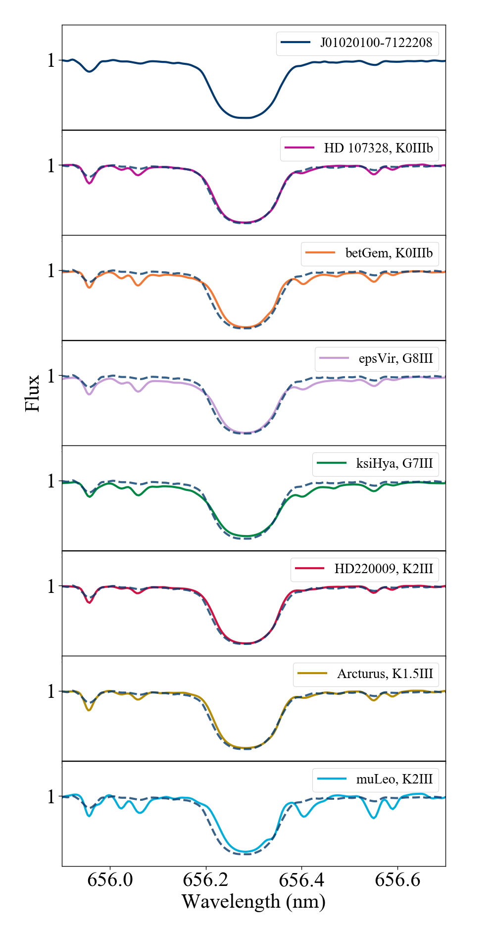
As a sanity check, we visually inspected at the profiles of the H lines, as was done previously in Neugent et al. (2018) and Massey et al. (2018). The first verification we did was to compare the regions containing H$\alpha$ and H$\beta$ lines of J01020100-7122208 with the H profiles of giant stars from our control sample, as well as those of the of Gaia Benchmark Stars (GBS) spectral library (Blanco-Cuaresma et al., 2014a). We chose that library because GBS have known spectral type and their parameters are used to validate several current spectroscopic surveys pipelines (Heiter et al., 2015b; Jofré et al., 2014, 2015; Hawkins et al., 2016; Jofré et al., 2017). For this purpose, we selected the giant GBS and considered the stellar classification of Heiter et al. (2015b). We did not use H lines located in the bluest regions because the spectrum of J01020100-7122208 is very noisy there and the spectra of GBS do not contain that region. The studied H lines are presented in Figure 8. We can see that likely there is a degeneracy in H$\alpha$, since the profile is very similar among all the stars, independently of their $T_{\mathrm{eff}}$. We can break the degeneracy with the other regions of the high resolution spectrum, because we use many iron lines of different ionisation and excitation states. We also note that the H profile of J01020100-7122208 agrees well with the profile of K0 stars from the GBS sample, and also with stars with $T_{\mathrm{eff}}$ of approximately 4500 K in the control sample.

Figure 8: Top left: Line profile of H$\beta$ for J01020100-7122208 (first spectrum) and for other giant stars in our control sample. Top right: Line profile of H$\alpha$ for J01020100-7122208 (first spectrum) and for other giant stars in our control sample. Bottom left: Line profile of H$\beta$ for J01020100-7122208 (first spectrum) and for other giant Gaia Benchmark stars. Bottom right: Line profile of H$\alpha$ for J01020100-7122208 (first spectrum) and for other giant Gaia Benchmark stars. In all panels containing control sample stars or GBS, the line profile of J01020100-7122208 is represented as blue dashed lines in order to help with the comparison.

B.2 Comparison with spectra

H I Balmer lines of FGK stars are useful when determining the temperature of stars (e.g. Searle & Oke (1962); Gehren (1981); Ruchti et al. (2013); Amarsi et al. (2018)). The wings of these lines are weakly dependent on the surface gravity of the star and the metallicity, being almost only sensitive to the temperature of the gas. Due to uncertainties in the models and observations, it is challenging to create H I profiles, but by exploring the wings of theses lines, we can obtain a good approximation of $T_{\mathrm{eff}}$ for a FGK-type star (Jofré et al., 2019). We used the synthetic grid from Amarsi et al. (2018), where the authors created a grid considering 3D and NLTE. The grid contains the regions of H$\alpha$ and H$\beta$. We chose the spectrum of a stars with $T_{\mathrm{eff}}=4500$ K, $\log g=1.5$ and $\mathrm{[Fe/H]}=-1.25$ to represent the results obtained in our work and a spectrum with $T_{\mathrm{eff}}=4800$ K, $\log g=2.0$ and $\mathrm{[Fe/H]}=-0.5$ to represent those of Massey et al. (2018). The profiles of H lines are presented in Figure 9. In this figure we observe that despite none of the synthetic spectra reproduce the line accurately (likely due to model limitations which affect the broadening of the lines), the wings of both H$\alpha$ and H$\beta$ are better represented by the stellar parameter values reported in our work.

Figure 9: Left: H$\beta$ profile of J01020100-7122208. Solid blue line represents the observed spectrum, the dashed green line represents a synthetic spectrum from the grid presented in Amarsi et al. (2018) with similar stellar parameters of those reported in our work and the dashed orange line represents another synthetic spectrum from the grid of Amarsi et al. (2018), but with similar stellar parameters of those presented in Massey et al. (2018). Right: H$\alpha$ profile of J01020100-7122208. Solid blue line represents the observed spectrum, the dashed green line represents a synthetic spectrum from the grid presented in Amarsi et al. (2018) with similar stellar parameters of those reported in our work and the dashed orange line represents another synthetic spectrum from the grid of Amarsi et al. (2018), but with similar stellar parameters of those presented in Massey et al. (2018).

References

- Abolfathi et al. (2018) Abolfathi B., et al., 2018, The Astrophysical Journal Supplement Series, 235, 42
- Aguado et al. (2021) Aguado D. S., et al., 2021, ApJ, 908, L8
- Alvarez & Plez (1997) Alvarez R., Plez B., 1997, arXiv preprint astro-ph/9710157
- Amarsi et al. (2018) Amarsi A. M., Nordlander T., Barklem P., Asplund M., Collet R., Lind K., 2018, Astronomy & Astrophysics, 615, A139
- Anders et al. (2017) Anders F., et al., 2017, Astronomy & Astrophysics, 597, A30
- Baglin et al. (2006) Baglin A., et al., 2006, in The CoRoT Mission Pre-Launch Status-Stellar Seismology and Planet Finding. p. 33
- Belokurov et al. (2018) Belokurov V., Erkal D., Evans N., Koposov S., Deason A., 2018, Monthly Notices of the Royal Astronomical Society, 478, 611
- Bennett & Bovy (2019) Bennett M., Bovy J., 2019, MNRAS, 482, 1417
- Bissantz et al. (2003) Bissantz N., Englmaier P., Gerhard O., 2003, Monthly Notices of the Royal Astronomical Society, 340, 949
- Blanco-Cuaresma (2019) Blanco-Cuaresma S., 2019, Monthly Notices of the Royal Astronomical Society, 486, 2075
- Blanco-Cuaresma et al. (2014a) Blanco-Cuaresma S., Soubiran C., Jofré P., Heiter U., 2014a, Astronomy & Astrophysics, 566, A98
- Blanco-Cuaresma et al. (2014b) Blanco-Cuaresma S., Soubiran C., Heiter U., Jofré P., 2014b, Astronomy & Astrophysics, 569, A111
- Borucki et al. (2010) Borucki W. J., et al., 2010, Science, 327, 977
- Brown et al. (2018) Brown A., et al., 2018, Astronomy & astrophysics, 616, A1
- Brown et al. (2021) Brown A. G., et al., 2021, Astronomy & Astrophysics, 649, A1
- Buchner et al. (2014) Buchner J., et al., 2014, Astronomy & Astrophysics, 564, A125
- Buder et al. (2020) Buder S., et al., 2020, Monthly Notices of the Royal Astronomical Society
- Busso et al. (1999) Busso M., Gallino R., Wasserburg G., 1999, Annual Review of Astronomy and Astrophysics, 37, 239
- Carollo et al. (2007) Carollo D., et al., 2007, Nature, 450, 1020
- Casamiquela et al. (2019) Casamiquela L., Tarricq Y., Soubiran C., Blanco-Cuaresma S., Jofré P., Heiter U., Maia M. T., 2019, arXiv preprint arXiv:1912.08539
- Chiappini et al. (2015) Chiappini C., et al., 2015, Astronomy & Astrophysics, 576, L12
- Choi et al. (2016) Choi J., Dotter A., Conroy C., Cantiello M., Paxton B., Johnson B. D., 2016, The Astrophysical Journal, 823, 102
- Combes (2013) Combes F., 2013, arXiv preprint arXiv:1309.1603
- Das et al. (2020) Das P., Hawkins K., Jofré P., 2020, Monthly Notices of the Royal Astronomical Society, 493, 5195
- Dotter (2016) Dotter A., 2016, The Astrophysical Journal Supplement Series, 222, 8
- Drimmel & Poggio (2018) Drimmel R., Poggio E., 2018, Research Notes of the American Astronomical Society, 2, 210
- Eisenhardt et al. (2020) Eisenhardt P. R. M., et al., 2020, ApJS, 247, 69
- Epstein et al. (2014) Epstein C. R., et al., 2014, The Astrophysical Journal Letters, 785, L28
- Feroz & Hobson (2008) Feroz F., Hobson M. P., 2008, Monthly Notices of the Royal Astronomical Society, 384, 449
- Feuillet et al. (2020) Feuillet D. K., Feltzing S., Sahlholdt C. L., Casagrande L., 2020, Monthly Notices of the Royal Astronomical Society, 497, 109
- Gaia Collaboration et al. (2016) Gaia Collaboration et al., 2016, A&A, 595, A1
- Gehren (1981) Gehren T., 1981, Astronomy and Astrophysics, 100, 97
- Gilmore & Wyse (1998) Gilmore G., Wyse R. F. G., 1998, AJ, 116, 748
- Gratton et al. (2003) Gratton R., Carretta E., Desidera S., Lucatello S., Mazzei P., Barbieri M., 2003, Astronomy & Astrophysics, 406, 131
- Gravity Collaboration et al. (2018) Gravity Collaboration et al., 2018, A&A, 615, L15
- Gray (2005) Gray D. F., 2005, The observation and analysis of stellar photospheres. Cambridge University Press
- Grevesse et al. (2007) Grevesse N., Asplund M., Sauval A., 2007, Space Science Reviews, 130, 105
- Gustafsson et al. (2008) Gustafsson B., Edvardsson B., Eriksson K., Jørgensen U. G., Nordlund Å., Plez B., 2008, Astronomy & Astrophysics, 486, 951
- Hansen et al. (2016) Hansen C. J., Rich R. M., Koch A., Xu S., Kunder A., Ludwig H.-G., 2016, Astronomy & Astrophysics, 590, A39
- Hawkins & Wyse (2018) Hawkins K., Wyse R. F., 2018, Monthly Notices of the Royal Astronomical Society, 481, 1028
- Hawkins et al. (2014) Hawkins K., Jofre P., Gilmore G., Masseron T., 2014, Monthly Notices of the Royal Astronomical Society, 445, 2575
- Hawkins et al. (2016) Hawkins K., et al., 2016, Astronomy & Astrophysics, 592, A70
- Heiter et al. (2015a) Heiter U., et al., 2015a, Physica Scripta, 90, 054010
- Heiter et al. (2015b) Heiter U., Jofré P., Gustafsson B., Korn A. J., Soubiran C., Thévenin F., 2015b, Astronomy & Astrophysics, 582, A49
- Hekker & Johnson (2019) Hekker S., Johnson J. A., 2019, Monthly Notices of the Royal Astronomical Society, 487, 4343
- Helmi et al. (2018) Helmi A., Babusiaux C., Koppelman H. H., Massari D., Veljanoski J., Brown A. G., 2018, Nature, 563, 85
- Holtzman et al. (2018) Holtzman J. A., et al., 2018, The Astronomical Journal, 156, 125
- Iwamoto et al. (1999) Iwamoto K., Brachwitz F., Nomoto K., Kishimoto N., Umeda H., Hix W. R., Thielemann F.-K., 1999, ApJS, 125, 439
- Izzard et al. (2018) Izzard R. G., Preece H., Jofre P., Halabi G. M., Masseron T., Tout C. A., 2018, Monthly Notices of the Royal Astronomical Society, 473, 2984
- Jofre & Weiss (2011) Jofre P., Weiss A., 2011, Astronomy & Astrophysics, 533, A59
- Jofré et al. (2014) Jofré P., et al., 2014, Astronomy & astrophysics, 564, A133
- Jofré et al. (2015) Jofré P., et al., 2015, Astronomy & astrophysics, 582, A81
- Jofré et al. (2016) Jofré P., et al., 2016, Astronomy & Astrophysics, 595, A60
- Jofré et al. (2017) Jofré P., et al., 2017, Astronomy & Astrophysics, 601, A38
- Jofré et al. (2019) Jofré P., Heiter U., Soubiran C., 2019, Annual Review of Astronomy and Astrophysics, 57, 571
- Jurić et al. (2008) Jurić M., et al., 2008, The Astrophysical Journal, 673, 864
- Kalirai (2012) Kalirai J. S., 2012, Nature, 486, 90
- Kelson (2003) Kelson D. D., 2003, Publications of the Astronomical Society of the Pacific, 115, 688
- Kobayashi & Nomoto (2009) Kobayashi C., Nomoto K., 2009, The Astrophysical Journal, 707, 1466
- Kobayashi et al. (2006) Kobayashi C., Umeda H., Nomoto K., Tominaga N., Ohkubo T., 2006, The Astrophysical Journal, 653, 1145
- Koposov (2020) Koposov S., 2020, Zenodo
- Koposov et al. (2020) Koposov S. E., et al., 2020, MNRAS, 491, 2465
- Koppelman et al. (2019) Koppelman H. H., Helmi A., Massari D., Price-Whelan A. M., Starkenburg T. K., 2019, Astronomy & Astrophysics, 631, L9
- Koppelman et al. (2020) Koppelman H. H., Bos R. O., Helmi A., 2020, arXiv preprint arXiv:2006.07620
- Kordopatis et al. (2020) Kordopatis G., Recio-Blanco A., Schultheis M., Hill V., 2020, Astronomy & Astrophysics, 643, A69
- Lindegren et al. (2021) Lindegren L., et al., 2021, A&A, 649, A2
- Mackereth et al. (2018) Mackereth J. T., et al., 2018, arXiv preprint arXiv:1808.00968
- Martig et al. (2015) Martig M., et al., 2015, Monthly Notices of the Royal Astronomical Society, 451, 2230
- Massey et al. (2018) Massey P., Levine S. E., Neugent K. F., Levesque E., Morrell N., Skiff B., 2018, The Astronomical Journal, 156, 265
- Matsuno et al. (2018) Matsuno T., Yong D., Aoki W., Ishigaki M. N., 2018, The Astrophysical Journal, 860, 49
- Matsuno et al. (2019) Matsuno T., Aoki W., Suda T., 2019, The Astrophysical Journal Letters, 874, L35
- Matsuno et al. (2020) Matsuno T., et al., 2020, arXiv preprint arXiv:2006.03619
- Matsuno et al. (2021) Matsuno T., Hirai Y., Tarumi Y., Hotokezaka K., Tanaka M., Helmi A., 2021, arXiv e-prints, p. arXiv:2101.07791
- Matteucci & Greggio (1986) Matteucci F., Greggio L., 1986, Astronomy and Astrophysics, 154, 279
- Matteucci et al. (2014) Matteucci F., Romano D., Arcones A., Korobkin O., Rosswog S., 2014, Monthly Notices of the Royal Astronomical Society, 438, 2177
- McMillan (2016) McMillan P. J., 2016, Monthly Notices of the Royal Astronomical Society, p. stw2759
- Montalbán et al. (2021) Montalbán J., et al., 2021, Nature Astronomy, pp 1–8
- Myeong et al. (2019) Myeong G., Vasiliev E., Iorio G., Evans N., Belokurov V., 2019, Monthly Notices of the Royal Astronomical Society, 488, 1235
- Neugent et al. (2010) Neugent K. F., Massey P., Skiff B., Drout M. R., Meynet G., Olsen K. A., 2010, The Astrophysical Journal, 719, 1784
- Neugent et al. (2018) Neugent K. F., Massey P., Morrell N. I., Skiff B., Georgy C., 2018, The Astronomical Journal, 155, 207
- Nissen & Schuster (2010) Nissen P. E., Schuster W. J., 2010, Astronomy & Astrophysics, 511, L10
- Nomoto et al. (2013) Nomoto K., Kobayashi C., Tominaga N., 2013, Annual Review of Astronomy and Astrophysics, 51, 457
- Onken et al. (2019) Onken C. A., et al., 2019, Publ. Astron. Soc. Australia, 36, e033
- Piffl et al. (2014) Piffl T., et al., 2014, Astronomy & Astrophysics, 562, A91
- Pignatari et al. (2010) Pignatari M., Gallino R., Heil M., Wiescher M., Käppeler F., Herwig F., Bisterzo S., 2010, The Astrophysical Journal, 710, 1557
- Plez (2012) Plez B., 2012, Astrophysics Source Code Library, pp ascl–1205
- Price-Whelan (2017) Price-Whelan A. M., 2017, The Journal of Open Source Software, 2
- Price-Whelan et al. (2018) Price-Whelan A. M., et al., 2018, The Astronomical Journal, 156, 123
- Randich & Magrini (2021) Randich S., Magrini L., 2021, Frontiers in Astronomy and Space Sciences, 8, 6
- Reid & Brunthaler (2004) Reid M. J., Brunthaler A., 2004, ApJ, 616, 872
- Riello et al. (2021) Riello M., et al., 2021, A&A, 649, A3
- Robitaille et al. (2013) Robitaille T. P., et al., 2013, Astronomy & Astrophysics, 558, A33
- Rossi et al. (2017) Rossi E. M., Marchetti T., Cacciato M., Kuiack M., Sari R., 2017, Monthly Notices of the Royal Astronomical Society, 467, 1844
- Ruchti et al. (2013) Ruchti G. R., Bergemann M., Serenelli A., Casagrande L., Lind K., 2013, Monthly Notices of the Royal Astronomical Society, 429, 126
- Schuster et al. (2012) Schuster W. J., Moreno E., Nissen P. E., Pichardo B., 2012, Astronomy & Astrophysics, 538, A21
- Searle & Oke (1962) Searle L., Oke J., 1962, The Astrophysical Journal, 135, 790
- Silva Aguirre et al. (2018) Silva Aguirre V., et al., 2018, Monthly Notices of the Royal Astronomical Society
- Skrutskie et al. (2006) Skrutskie M. F., et al., 2006, AJ, 131, 1163
- Tayar et al. (2017) Tayar J., et al., 2017, ApJ, 840, 17
- Timmes et al. (1995) Timmes F., Woosley S., Weaver T. A., 1995, The Astrophysical Journal Supplement Series, 98, 617
- Tinsley (1979) Tinsley B., 1979, The Astrophysical Journal, 229, 1046
- Tody (1993) Tody D., 1993, in Hanisch R. J., Brissenden R. J. V., Barnes J., eds, Astronomical Society of the Pacific Conference Series Vol. 52, Astronomical Data Analysis Software and Systems II. p. 173
- Tolstoy et al. (2009) Tolstoy E., Hill V., Tosi M., 2009, Annual Review of Astronomy and Astrophysics, 47, 371
- Vincenzo et al. (2019) Vincenzo F., Spitoni E., Calura F., Matteucci F., Silva Aguirre V., Miglio A., Cescutti G., 2019, Monthly Notices of the Royal Astronomical Society: Letters, 487, L47
- Woosley & Weaver (1995) Woosley S., Weaver T. A., 1995, Technical report, The evolution and explosion of massive Stars II: Explosive hydrodynamics and nucleosynthesis. Lawrence Livermore National Lab., CA (United States)
- Yong et al. (2016) Yong D., et al., 2016, Monthly Notices of the Royal Astronomical Society, 459, 487
- Zhang et al. (2021) Zhang H., et al., 2021, arXiv preprint arXiv:2102.05999