Green functions for a chain subjected to a uniformly varying field in the context of electron transmission

Abstract

On the basis of the tight-binding formalism and Green function technique we obtain all the Green functions matrix elements for a biased chain with a linear variation of the electron on-site energy. Their dependence on the system parameters is analyzed in the context of through-molecule electron transport.

I Introduction

During last decades, fabrication of different molecular contacts of the type ”metal-molecular system-metal” has received an impressive experimental development allowing high precision measurements of electrical current through single molecules, nanotubes, self-assembled monolayers, nanometer-size dielectric and semiconductor films. However, interpretation of these experiments using Landauer concept of conductance requires, as a rule, the use of computational simulations of molecular electronic structure. Such studies often give quite limited and method-dependent information, which stimulates the development of analytical approaches to investigation of electrical properties of molecular contacts.

In the present report, we use the derivation of the transmission coefficient $T(E,V)$, the ratio of the transmitted to incident electron flux at the given energy $E$ and applied voltage $V$, in terms of the coupling function matrix [1, 2, 3, 4, 5, 6]. This matrix is determined by the ideal lead Green’s functions and molecule-lead interaction matrix. We use the formulation used in [4] whose benefits make it possible to describe molecular contacts exactly and with the use of realistic model Hamiltonians. Thus, we use the exact analytical expression of the transmission coefficient for a three-dimensional 3D lead modeled by a cubic semiinfinite lattice with an arbitrary number of atoms in the surface and subsurface layers interacting with the molecule [3].

In 1960, Wannier introduced the concept of electron energy quantization in solids subjected to a constant homogeneous electric field [7, 8]. Actually, his concept was formulated for an infinite monoatomic chain described in the Wannier tight-binding approximation. It can be considered as the theory of Stark effect for a chain of interacting single-level atoms. Therefore, the obtained electron spectrum was named a Wannier-Stark ladder or WS quantization of electron energy, $E_{\mu}=\mu\varepsilon$, $\mu$ is an integer. The field parameter $\varepsilon$ ($-\varepsilon$) determines the change of the electron potential energy from one atom to the next along (against) the field.

A number of accurate explicit expressions showing the electric-field effects on the chain electron spectrum have been derived in [4, 9, 10, 11, 12, 13, 14, 15, 16, 17]. The polynomial representation of the exact solution of the spectral problem for the field-affected $\cal N$-atom long tight-binding chain [18] was obtained in the context of through-molecule transport.

In this paper, we report all explicit expressions for the matrix elements of the Green functions for a biased chain with a linear variation of the electron on-site energy derived from the exact characteristic equation of Hamiltonian matrix for ${\cal N}$-length atomic chain. The obtained results are used for obtaining an explicit expression of the transmission coefficient of electrons through a spatially finite tilted band. It reveals the resonance structure of the transmission spectrum and its dependence on the characteristic parameters of the system.

II Transmission Coefficient

Consider a metal wire interrupted by a scattering region but otherwise ideal in the sense that in the absence of the imperfection, electrons could flow freely along the wire. Assume that, as sketched in Fig. 1a, it is a molecule, which is coupled in some way to the left and right parts of the wire (the left and right leads), that plays the role of the imperfection. In the framework of the Landauer-Büttiker theory [19, 20, 21] the transmission probability is directly related to the current-voltage relation. For the efficient computation and analytic analysis of the transmission coefficient, the Green function technique is known to be particularly useful for the development of efficient computational schemes. In work [22] it was proposed to describe the tunnel current in metal-insulator-metal heterostructures using the Green function language. Later on their treatment has been reformulated in a number of physical contexts to examine, in particular, the quantum conductance of molecular wires [9, 10, 11, 12, 13, 3].

In the framework of the Green function formalism, $T(E,V)$ can be conveniently expressed in terms of the Green functions referring to the noninteracting left and right leads and the scattering region. To find $T(E,eV)$, we concretize our model as follows. In the bra-ket notation, $|{\bf n}\rangle\equiv a^{+}_{\bf n}|0\rangle=a^{+}_{n_{x}}a^{+}_{\perp}|0\rangle$ = $a^{+}_{n_{x}}a^{+}_{n_{y}}a^{+}_{n_{z}}|0\rangle$, $\langle{\bf n}|{\bf n}^{\prime}\rangle=\delta_{{\bf n},{\bf n}^{\prime}}$, the Hamiltonian of the system ”left lead - molecular contact - right lead” depicted in Fig. 1 reads

$$\hat{H}=\hat{H}^{\rm L}+\hat{H}^{\rm cont}+\hat{H}^{\rm R}+\hat{H}^{\rm int}.$$ (1)

Figure 1 explains the model parameters and shows the potential profile on the electron way from left to right electrodes. We assume that in the absence of the interaction between the left/right leads and the contact the eigenstates $\Psi^{\mu}$ of the Hamiltonian operator $\hat{H}^{\mu}$ of the leads and the contact ($\mu={\rm L},{\rm R}$, and cont, respectively) can be expanded in a series of the respective basis set of atomic orbitals $\Psi^{\mu}=\sum_{{\mathbf{n}}\in{\mathbf{n}}_{\mu}}\psi^{\mu}_{\mathbf{n}}|{\mathbf{n}}\rangle$. We also treat Hamiltonians $\hat{H}^{\rm L}$, $\hat{H}^{\rm R}$ which describe the leads, as free electron Hamiltonians of semi-infinite cubic lattices with the electron on-site energy $\varepsilon$ and the hopping integral between the nearest-neighbor atoms denoted by $-\beta$ ($\beta>0$). Thus, the energy of transmitted waves is

$$E(k_{j_{y},j_{z}})=6\beta-2\beta\left[\cos(k_{j_{y},j_{z}})+\cos\left(\xi_{y}\right)+\cos(\xi_{z})\right],\quad\xi_{(y,z)}\equiv\frac{\pi j_{(y,z)}}{N_{(y,z)}+1}\quad j_{(y,z)}=1,\dots,N_{(y,z)},$$ (2)

where $k_{j_{y},j_{z}}$ is real (imaginary) for propagating (evanescent) modes.

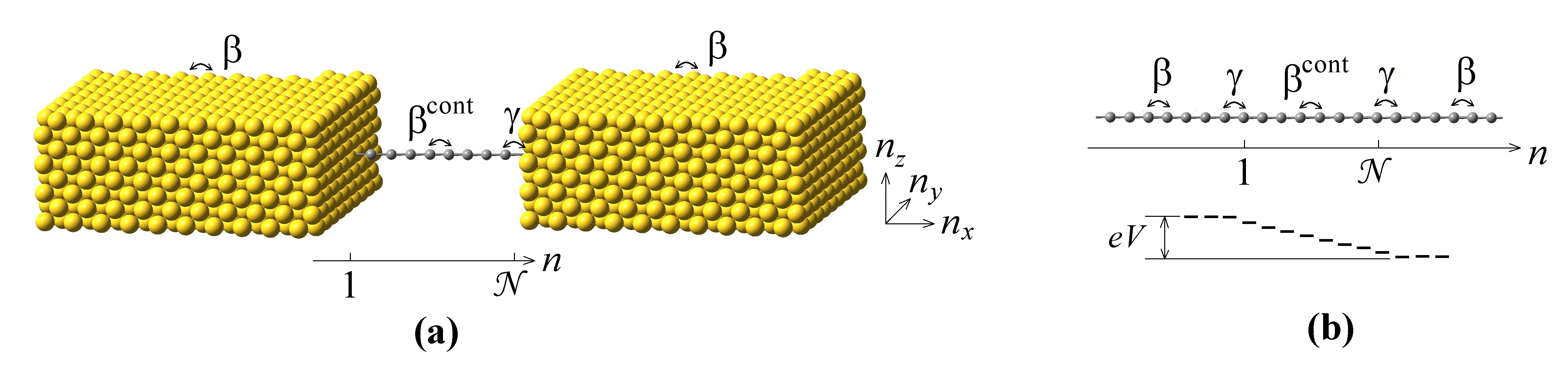
Figure 1: (a). Fragments of semi-infinite (in $n_{x}$ direction) left and right leads with a molecular chain in between. The binding atoms of the chain are in on-top position. Energies of electron transfer between adjacent atoms are $\beta$ in the leads, $\beta^{\rm cont}$ in the molecular chain, and $\gamma$ on the electrode-molecule interface. (b) One-dimensional case, $N_{y}=N_{z}=1$.

The left-to-right drop of the applied potential $eV$ is taken into account as a shift of the site energies of each atom by the field parameter $\varepsilon_{F}=eFa/\beta$, where $e$ is the absolute value of electron charge, $F$ is the electric field strength, and $a$ is the lattice constant. Thus, it is assumed that the potential difference between the left and right electrodes drops linearly inside the contact: $eV=\varepsilon_{F}({\cal N}+1)$, and the Hamiltonian of molecular chain has the form

$$\hat{H}^{\rm cont}=\sum_{n=1}^{\cal N}\left\{(\varepsilon^{\rm cont}-n\varepsilon_{F})a^{+}_{n}a_{n}-\beta^{\rm cont}\big{[}(1-\delta_{n,1})a^{+}_{n-1}+(1-\delta_{n,{\cal N}})a^{+}_{n+1}\big{]}a_{n}\right\}.$$ (3)

We consider a simplified model of metal-molecular interaction which involves only two of all molecule atoms: these binding atoms have coordinates $n=1$ and $n=\cal N$. The interaction operator is then given by

$$\hat{H}^{\rm int}=\gamma\sum_{{\mathbf{n}}\in{\mathbf{n}}_{\rm L}}|1\rangle\langle{\mathbf{n}}|+\gamma\sum_{{\mathbf{n}}\in{\mathbf{n}}_{\rm R}}|{\cal N}\rangle\langle{\mathbf{n}}|,$$ (4)

i.e., the parameter $\gamma$ accounts to the difference between the electron transfer rates from contact to electrodes and backward.

By definition, the transmission coefficient is equal to the ratio of the transmitted electron flux to the incident flux. The derivation of the transmission coefficient is well known [1, 2, 3, 4]. Due to simplifying model assumptions, this principal quantity can be obtained in a fully analytical form via solving the Lippman-Schwinger equation with the Hamiltonian $\hat{H}$. Here, we use $T(E,eV)$ in the following form:

$$T(E,eV)=4{\rm Im}(A^{\rm L}){\rm Im}(A^{\rm R})\left|\dfrac{G^{\mathstrut\rm cont}_{1,{\cal N}}}{\left(1-A^{\rm L}G^{\mathstrut\rm cont}_{1,1}\right)\left(1-A^{\rm R}G^{\mathstrut\rm cont}_{{\cal N},{\cal N}}\right)-A^{\rm L}A^{\rm R}(G^{\mathstrut\rm cont}_{1,{\cal N}})^{2}}\right|^{2},$$ (5)

where $G^{\mathstrut\rm cont}_{n,n^{\prime}}$ are the Green functions for the Hamiltonian (3) and the coupling functions $A^{\rm L},A^{\rm R}$ are defined as follows:

$$\begin{split}A^{({\rm L},{\rm R})}&=\gamma^{2}\sum_{{\mathbf{n}},{\mathbf{n}^{\prime}}\in{\mathbf{n}}_{({\rm L},{\rm R})}}G^{({\rm L},{\rm R})}_{{\mathbf{n}},{\mathbf{n}^{\prime}}},\\ G^{({\rm L},{\rm R})}_{1,n_{y},n_{z};1,n_{y}^{\prime},n_{z}^{\prime}}&=-\dfrac{1}{\beta}\dfrac{4}{(N_{y}+1)(N_{z}+1)}\sum_{j_{y}=1}^{N_{y}}\sum_{j_{z}=1}^{N_{z}}e^{ik^{({\rm L},{\rm R})}_{j_{y},j_{z}}}\sin(\xi_{y}n_{y})\sin(\xi_{z}n_{z})\sin(\xi_{y}n_{y}^{\prime})\sin(\xi_{z}n_{z}^{\prime}).\end{split}$$ (6)

Finding the transmission coefficient for the model specified by the Hamiltonian operator in Eq. (3) requires the knowledge of the Green’s function matrix elements appeared in Eq. (5). They are found in the next section. From now and on the model parameters $\varepsilon$, $\varepsilon^{\rm cont}$, $\beta^{\rm cont}$, $\gamma$, and $\varepsilon_{F}$ will be expressed using $\beta$ as the unit of energy.

III Green’s functions for a tilted chain in the framework of the tight-binding model

The system of equations for finding the required Green’s functions reads

$$\left(E-\varepsilon^{\rm cont}+n\varepsilon_{F}\right)G^{\mathstrut\rm cont}_{n,n^{\prime}}=-\beta^{\rm cont}[G^{\mathstrut\rm cont}_{n-1,n^{\prime}}(1-\delta_{n,1})+G^{\mathstrut\rm cont}_{n+1,n^{\prime}}(1-\delta_{n,N})]+\delta_{n,n^{\prime}},\quad n,n^{\prime}=1,\dots,{\cal N}.$$ (7)

To find all the matrix elements $G^{\mathstrut\rm cont}_{n,n^{\prime}}$, it is convenient to use the generating functions method. We define the generating function as follows:

$${\cal G}_{n^{\prime}}(\varphi)=\sum_{n=1}^{\cal N}G^{\mathstrut\rm cont}_{n,n^{\prime}}(E,eV)e^{in\varphi}.$$ (8)

It can be verified by direct substitution that ${\cal G}(\varphi)$ satisfies the following differential equation:

$$(E-\varepsilon^{\rm cont}-2\beta^{\rm cont}\cos\varphi){\cal G}_{n^{\prime}}(\varphi)+i\dfrac{\beta^{\rm cont}}{a{\cal F}}\frac{d{\cal G}_{n^{\prime}}(\varphi)}{d\varphi}=e^{in^{\prime}\varphi}-G^{\mathstrut\rm cont}_{1,n^{\prime}}(E,eV)-e^{i({\cal N}+1)\varphi}G^{\mathstrut\rm cont}_{{\cal N},n^{\prime}}(E,eV).$$ (9)

Solving this linear differential equation allows to express the solution of (7) in terms of Bessel functions of the first and second kind:

$$\begin{split}&G^{\mathstrut\rm cont}_{n,n^{\prime}}(E,eV)=-\frac{\pi}{\varepsilon_{F}\big{[}J_{\nu}(z)Y_{\nu-{\cal N}-1}(z)-J_{\nu-{\cal N}-1}(z)Y_{\nu}(z)\big{]}}\\[20.0pt] &\times\left\{\begin{array}[]{l}\big{[}J_{\nu-n}(z)Y_{\nu-{\cal N}-1}(z)-J_{\nu-{\cal N}-1}(z)Y_{\nu-n}(z)\big{]}\big{[}J_{\nu}(z)Y_{\nu-n^{\prime}}(z)-J_{\nu-n^{\prime}}(z)Y_{\nu}(z)\big{]},\quad n\geq n^{\prime},\\ \\ n\leftrightarrow n^{\prime},\quad n\leq n^{\prime},\quad z=\dfrac{2\beta^{\rm cont}}{\varepsilon_{F}},\quad\nu=-(E-\varepsilon^{\rm cont})\dfrac{{\cal N}+1}{eV}=-(E-\varepsilon^{\rm cont})\dfrac{1}{\varepsilon_{F}}.\\ \end{array}\right.\end{split}$$ (10)

For the particular values of $n,n^{\prime}=1,{\cal N}$, Eq. (10) gives the expressions for the Green’s functions used in the definition of the transmission coefficient $T(E,eV)$:

$${\cal D}_{G}(E,eV)G^{\mathstrut\rm cont}_{1,1}(E,eV) =J_{\nu-1}(z)Y_{\nu-{\cal N}-1}(z)-Y_{\nu-1}(z)J_{\nu-{\cal N}-1}(z)\equiv\tilde{G}_{1,1},$$

$${\cal D}_{G}(E,eV)G^{\mathstrut\rm cont}_{{\cal N},{\cal N}}(E,eV) =J_{\nu}(z)Y_{\nu-{\cal N}}(z)-Y_{\nu}(z)J_{\nu-{\cal N}}(z)\equiv\tilde{G}_{{\cal N},{\cal N}},$$

$${\cal D}_{G}(E,eV){G}^{\mathstrut\rm cont}_{1,{\cal N}}(E,eV) =\dfrac{1}{\pi}\dfrac{\varepsilon_{F}}{\beta^{\rm cont}}\equiv\tilde{G}_{1,{\cal N}},$$

$$Q(E,eV) ={\cal D}_{G}(E,eV)\left\{{G}^{\mathstrut\rm cont}_{1,1}(E,eV){G}^{\mathstrut\rm cont}_{{\cal N},{\cal N}}(E,eV)-\big{[}{G}^{\mathstrut\rm cont}_{1,{\cal N}}(E,eV)\big{]}^{2}\right\}$$

$$=\dfrac{1}{\beta^{\rm cont}}\left[J_{\nu-1}(z)Y_{\nu-{\cal N}}(z)-Y_{\nu-1}(z)J_{\nu-{\cal N}}(z)\right],$$ (11)

and

$${\cal D}_{G}(E,eV)=-\beta^{\rm cont}\left[J_{\nu}(z)Y_{\nu-{\cal N}-1}(z)-Y_{\nu}(z)J_{\nu-{\cal N}-1}(z)\right].$$ (12)

Note that for the case ${\cal N}=1$, making use of the well-known relations for the Bessel functions

$$\begin{split}J_{\nu-1}(z)Y_{\nu-2}(z)&-Y_{\nu-1}(z)J_{\nu-2}(z)=\dfrac{2}{\pi z},\\ J_{\nu-1}(z)+J_{\nu+1}(z)&=\dfrac{2\nu}{z}J_{\nu}(z),\quad Y_{\nu-1}(z)+Y_{\nu+1}(z)=\dfrac{2\nu}{z}Y_{\nu}(z),\end{split}$$ (13)

in Eqs. (III), (12), we obtain the evident relation

$$G^{\mathstrut\rm cont}_{1,1}(E,eV)=\dfrac{1}{E-(\varepsilon^{\rm cont}-eV/2)}.$$ (14)

Relations (10) give analytical expressions for the Green functions for a biased linear chan which can be used for analytical modeling in a great number of applications. Substituting Eqs. (III) in Eq. (5) allows to find the transmission coefficient for the system depicted in Fig. 1. In the next section, we use these results to derive $T(E,eV)$ for the case $N_{y}=N_{z}=1$, i.e., for an atomic chain shown in Fig. 1b.

IV One-dimensional case

For the case $N_{y}=N_{z}=1$, our model corresponds to an atomic chain shown in Fig. 1b. The site energy along the chain equals 2 (to recall, in $\beta$ units) for $n_{x}\leq 0$, $2-eV$ for $n_{x}>{\cal N}$, and $2-\varepsilon_{F}n$, $\varepsilon_{F}=eV/(N+1)$ for $n\in\overline{1,\cal N}$ in, respectively, the left and right electrodes and contact. The eigen energies (2) for Hamiltonian (1) simplify in this case to

$$E=2\left(1-\cos k^{\rm L}\right)=2\left(1-\cos k^{\rm R}\right)-eV,\quad 0\leq k^{\rm L},k^{\rm R}\leq\pi,$$ (15)

with the wave vectors in units of the inverse interatomic distance $a^{-1}$. Relation (5) is rewritten as follows:

$$T(E,eV)=\dfrac{4\gamma^{4}\sin k^{\rm L}\sin k^{\rm R}(G^{\mathstrut\rm cont}_{1,{\cal N}})^{2}}{\left|1+\gamma^{2}\left(e^{ik^{\rm L}}G^{\mathstrut\rm cont}_{1,1}+e^{ik^{\rm R}}G^{\mathstrut\rm cont}_{{\cal N},{\cal N}}\right)+\gamma^{4}e^{i(k^{\rm L}+k^{\rm R})}\left[G^{\mathstrut\rm cont}_{1,1}G^{\mathstrut\rm cont}_{{\cal N},{\cal N}}-\left(G^{\mathstrut\rm cont}_{1,{\cal N}}\right)^{2}\right]\right|^{2}}.$$ (16)

Using relations for the Green functions (III), after some algebra, we get

$${\cal D}_{T}T(E,eV) =4\gamma^{4}\sin k^{\rm L}\sin k^{\rm R}\tilde{G}_{1,{\cal N}}^{2},$$

$${\cal D}_{T} \equiv\Big{[}{\cal D}_{G}+\gamma^{2}\left(\cos k^{\rm L}\tilde{G}_{1,1}+\cos k^{\rm R}\tilde{G}_{{\cal N},{\cal N}}\right)+\gamma^{4}\cos\left(k^{\rm L}-k^{\rm R}\right)Q(E,eV)\Big{]}^{2}$$

$$\quad+\gamma^{4}\Big{[}\sin k^{\rm L}\tilde{G}_{1,1}-\sin k^{\rm R}\tilde{G}_{{\cal N},{\cal N}}+\gamma^{2}\sin\left(k^{\rm L}-k^{\rm R}\right)Q(E,eV)\Big{]}^{2}+4\gamma^{4}\sin k^{\rm L}\sin k^{\rm R}\tilde{G}^{2}_{1,{\cal N}}.$$ (17)

The condition of transmission without backscattering, $T(E,eV)=1$, directly follows from Eq. (IV):

$$\Big{[}\gamma^{-2}{\cal D}_{G}+\cos k^{\rm L}\tilde{G}_{1,1} +\cos k^{\rm R}\tilde{G}_{{\cal N},{\cal N}}+\gamma^{2}\cos\left(k^{\rm L}-k^{\rm R}\right)Q(E,eV)\Big{]}^{2}$$

$$+\Big{[}\sin k^{\rm L}\tilde{G}_{1,1}-\sin k^{\rm R}\tilde{G}_{{\cal N},{\cal N}}+\gamma^{2}\sin\left(k^{\rm L}-k^{\rm R}\right)Q(E,eV)\Big{]}^{2}=0.$$ (18)

In the particular case, $\beta^{\rm cont}=1$ and $eV=0$ (and, consequently, $k^{\rm L}=k^{\rm R}=k$), Eq. (IV), repeats the result obtained earlier [4]:

$$T(E,0)=\dfrac{4\gamma^{4}\sin^{4}k}{\big{\{}[\sin({\cal N}+1)k]-2\gamma^{2}\cos k\sin{\cal N}k+\gamma^{4}\sin[({\cal N}-1)k]\big{\}}^{2}+4\gamma^{4}\sin^{4}k}.$$ (19)

Expression (IV), though much simpler than Eq.(5), still remains fairly complicated. However, for the case of small potential difference, $eV<<1$, it can be significantly simplified with the help of the approximation similar to that used in [16]. Namely, for any coupling parameter $\gamma$ and any $\cal N$, the transmission coefficient $T(E,eV)$ can be approximated as follows:

$$T(E,eV)\approx\dfrac{4\gamma^{4}}{4\gamma^{4}+(1-\gamma^{4})^{2}\sin^{2}\left[p+\dfrac{{\cal N}+1}{2}\left(E-2+\dfrac{eV}{2}\right)\right]},\quad p\equiv\dfrac{\pi}{4}[(-1)^{\cal N}+1].$$ (20)

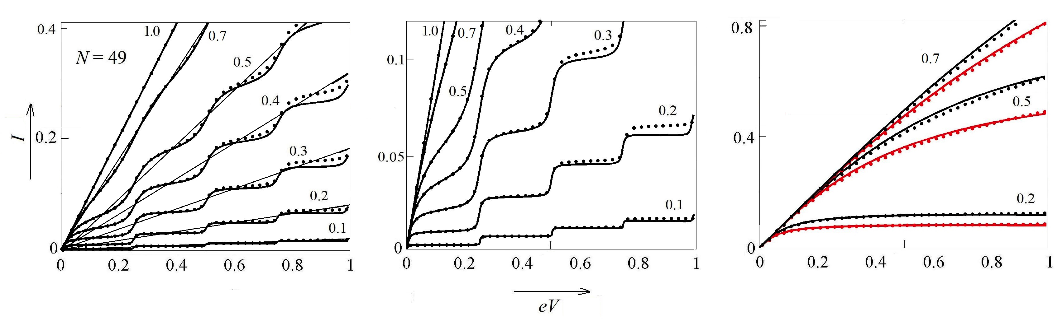
Figure 2: Left panel: The exact dependence $I(eV)$, Eq. (21) – solid lines, and its approximation (22) – dotted lines, calculated for $N=49$ and $\gamma=0.1,0.2,0.3,0.4,0.5,0.7,1.0$. Central panel: Enlarged dependences shown on the left panel. Right panel: The same dependences for $N=3$ (black), $N=5$ (red) and $\gamma=0.2,0.5$, and 0.7.

Following the Landauer-Büttiker theory [19, 20], we express the current-voltage relation via the transmission coefficient in the form

$$I(eV)=\dfrac{2e}{h}\int\limits_{\max\left(0,2-eV\right)}^{\min\left(2,4-eV\right)}T(E,eV)dE.$$ (21)

The limits of integration $[2-eV,2]$, $0\leq eV\leq 2$ and $[0,4-eV]$, $2\leq eV\leq 4$ correspond to the nonzero values of the transmission coefficient dictated by the Pauli exclusion principle. Since, for the condition $eV<<1$, the obtained approximation for the transmission coefficient (20) admits the exact integration, we derive an explicit expression for the current as a function of the potential difference, $\gamma$, and $\cal N$:

$$I(eV)=\dfrac{2e}{h}\dfrac{8\gamma^{2}}{({\cal N}+1)(1+\gamma^{4})}\arctan\left\{\dfrac{1+\gamma^{4}}{2\gamma^{2}}\tan\left[p+\dfrac{({\cal N}+1)eV}{4}\right]\right\},\quad eV\lesssim 1.$$ (22)

As illustrated in Fig. 2, this approximation works reasonably well in the interval $0<eV\lesssim 1$. Thus, simple analytic approximation (22) satisfactory reproduces the current-voltage dependences for molecular contact depicted in Fig. 1 as functions of the coupling parameter and the contact length for the potential differences varying from zero to several electron-volts.

References

[1]
Mujica, M. Kemp, and M. A. Ratner, J. Chem. Phys. 101,
6849 (1994); 101, 6856 (1994).
[2]
S. Datta, Electronic Transport In Mesoscopic Systems. Cambridge University Press, Cambridge (1995).
[3]
A. Onipko and L. Malysheva, Phys. Rev. B, 62, 10480 (2000).
[4]
A. Onipko and L. Malysheva, Coherent electron
transport in molecular contacts: a case of tractable modeling. In:
Handbook on Nano- and Molecular Electronics. Chapter 23. CRC Press (2007).
[5]
A. Nitzan, Annu. Rev. Phys. Chem., 52, 681 (2001).
[6]
S. Datta, Quantum Transport: Atom to Transistor. Cambridge University Press, Cambridge (2005).
[7]
G. H. Wannier, Phys. Rev. 117, 432 (1960).
[8]
G. H. Wannier, Rev. Mod. Phys. 34, 645 (1962).
[9]
G. C. Stey and G. Gusman, J. Phys. C: Solid State Phys. 6, 650 (1973).
[10]
H. Fukuyama, R. A. Bari, and H. C. Fogedby, Phys. Rev. B 8, 5579 (1973).
[11]
V. M. Yakovenko and H.-S. Goan, Phys. Rev. B 58, 8002 (1998).
[12]
Yu. B. Gaididei and A. A. Vakhnenko, Phys. Status Solidi B, 121, 239 (1984).
[13]
S. G. Davison, R. A. English, A. L. Mis̆ković, F. O. Goodman, A. T. Amos, and B. L. Burrows, J. Phys.: Condens. Matter 9, 6371 (1997).
[14]
A. Onipko and L. Malysheva, Solid State Commun. 118, 63 (2001).
[15]
A. Onipko and L. Malysheva, Phys. Rev. B, 63, 235410 (2001).
[16]
A. Onipko and L. Malysheva, Phys. Rev. B, 64, 195131 (2001).
[17]
A. Onipko and L. Malysheva, Phys. Status Solidi B, 1700558 (2018).
[18]
L. I. Malysheva, Ukr. Fiz. Zh. 45, 1475 (2000).
[19]
R. Landauer, IBM J. Res. Dev. 1, 323 (1957); Philos. Mag. 21,
683 (1970).
[20]
M. Büttiker, Y. Imry, R. Landauer, and S. Pinhas, Phys. Rev. B
31, 6207 (1985).
[21]
Y. Imry, Introduction to Mesoscopic Physics. Oxford University Press, Oxford, 2002.
[22]
C. Caroli, R. Combescot, P. Nozières, and D. Saint-James, J.
Phys. C 4, 916 (1971).