Thermal and nonthermal emission in the optical-UV spectrum of PSR B0950+08

Abstract

Based on recent Hubble Space Telescope (HST) observations in far-UV and groundbased observations in optical bands, Pavlov and colleagues have revealed a thermal component in the spectrum of the old pulsar B0950+08 (spin-down age 17.5 Myr) and estimated a neutron star (NS) surface temperature of $(1$–$3)\times 10^{5}$ K. Our new HST observations in the optical have allowed us to resolve the pulsar from a close-by galaxy and measure the optical fluxes more accurately. Using the newly measured fluxes and a new calibration of the HST’s far-UV detector, we fit the optical-UV pulsar’s spectrum with a model that consists of a nonthermal power-law ($f_{\nu}\propto\nu^{\alpha}$) and a thermal blackbody components. We obtained the spectral slope $\alpha=-0.3\pm 0.3$, considerably flatter than found from groundbased observations, and the best-fit temperature in the range of $(6$–$12)\times 10^{4}$ K (as seen by a distant observer), depending on interstellar extinction and NS radius. The temperature is lower than reported previously, but still much higher than predicted by NS passive cooling scenarios for such an old pulsar. This means that some heating mechanisms operate in NSs, e.g., caused by interaction of the faster rotating neutron superfluid with the slower rotating normal matter in the inner crust of the NS.

1 Introduction

Born very hot, neutron stars (NSs) lose their thermal energy via neutrino and photon emission. Since the cooling rate depends on the composition and state of matter in the NS interiors, the study of thermal evolution of NS is an important tool for understanding the fundamental properties of matter. While the thermal evolution of young NSs in the neutrino-dominated cooling era ($\tau\lesssim 1$ Myr) has been well investigated (see Yakovlev & Pethick 2004 and Page et al. 2009 for reviews), the thermal evolution of older NSs remains virtually unexplored. If an NS just cools passively, then its surface temperature is expected to drop very fast in the photon-dominated cooling era ($\tau\gtrsim 1$ Myr), going below $10^{4}$ K by $\tau\sim 10$ Myr. However, it has long been recognized that various heating processes may slow (or even reverse) the cooling (e.g., Gonzalez & Reisenegger 2010, and references therein).

For instance, interaction of vortex lines of the faster rotating neutron superfluid with the slower rotating normal matter in the inner NS crust can heat the NS surface up to temperatures of a few times $10^{5}$ K at an age of $\sim 10$–100 Myr (Alpar et al. 1984; Shibazaki & Lamb 1989; Larson & Link 1999; Gonzalez & Reisenegger 2010). This “frictional heating” mechanism can be explored in observations of thermal emission from old NSs. An optimal range for such observation is far-UV (FUV) because the thermal flux is higher there at the expected temperatures and because optical spectrum can be dominated by magnetospheric emission if the NS is a rotation-powered pulsar. Since FUV emission is unobservable from the ground, observational studies of heating mechanisms and thermal evolution of NSs can only be done with the Hubble Space Telescope (HST; Pavlov 1992). Since NSs in general, and the thermal evolution of NSs in particular, are not the favorite subjects of HST panels, very few proposals on this topic have been accepted in 30 years of the HST era. Nevertheless, those few accepted and executed programs led to important discoveries, one of which was the observational confirmation of NS heating in two old pulsars – the millisecond (recycled) pulsar J0437–4715 and the “classical” (nonrecycled) pulsar B0950+08. New observations of the latter is the main subject of this paper.

PSR B0950+08 (= J0953+0755; B0950 hereafter) is a solitary radio and X-ray pulsar, one of the first pulsars discovered (Pilkington et al., 1968). It has the period $P=253$ ms, spin-down energy loss rate $\dot{E}=5.6\times 10^{32}$ erg s^-1, spin-down age $\tau_{\rm sd}=17.5$ Myr, and surface magnetic field $B\sim 2.4\times 10^{11}$ G (Manchester et al., 2005). The parallax distance $d=262\pm 5$ pc and proper motion $\mu_{\alpha}=-2.08\pm 0.08$ mas yr^-1, $\mu_{\delta}=29.46\pm 0.07$ mas yr^-1 correspond to the transverse velocity $V_{\perp}=36.6\pm 0.7$ km s^-1 (Brisken et al., 2002).

Optical–UV emission from B0950 was discovered by Pavlov et al. (1996) in HST observations with the Faint Object Camera in a long-pass filter F130LP (pivot wavelength 3438 Å).They measured a mean spectral flux density $\overline{f}_{\nu}=51\pm 3$ nJy in this filter. In observations with the Subaru telescope Zharikov et al. (2002) measured the flux density of $60\pm 9$ nJy in the B filter. Observations with the VLT/FORS1 telescope gave the B, V, R and I flux densities of $60\pm 17$, $45\pm 6$, $91\pm 8$ and $78\pm 11$ nJy, respectively (Zharikov et al., 2004). The large scatter in the flux values was likely caused by contamination, particularly in the I and R bands, from a red extended object at about $1^{\prime\prime}$ north of the pulsar. Despite this scatter, it is clear that the optical emission from B0950 is nonthermal. Fitting these flux densities with a power-law (PL) model, $f_{\nu}\propto\nu^{\alpha}$, Zharikov et al. (2004) obtained $\alpha=-0.65\pm 0.40$.

Table 1: HST observations of PSR B0950+08

Visit	Start time	Instrument	Filter	$\lambda_{p}$	$\rm W_{eff}$	Dither points	Total exposure
				(Å)	(Å)		(s)
1	2020-05-15  11:07:49	WFC3/UVIS	F475X	4936	1981	4	2420
2	2020-06-05  04:25:00	ACS/WFC	F775W	7693	1379	3	3726
3	2021-03-06  15:23:40	ACS/WFC	F775W	7693	1379	2	2434

In a search for thermal emission from the NS surface, Pavlov et al. (2017) observed B0950 with the Solar-Blind Channel (SBC) of the HST Advanced Camera for Surveys (ACS). The observations were carried out with the F125LP and F140LP long-pass filters, with pivot wavelengths 1438 Å and 1528 Å. The corresponding mean flux densities, $\overline{f}_{\nu}=109\pm 6$ and $83\pm 14$ nJy, substantially exceeded the extrapolation of the optical PL spectrum into this FUV range. Therefore, Pavlov et al. (2017) conclude that the FUV excess is due to the thermal emission. Fitting the optical-FUV flux densities with a two-component PL + blackbody (BB) model, they found a PL slope $\alpha\sim-1.2$ and a brightness temperature in the range of $(1$–$3)\times 10^{5}$ K, depending on interstellar extinction and NS radius. These temperatures are much higher than predicted by NS cooling models for such an old pulsar, which means that some heating mechanisms operate in NSs.

This conclusion, however, was based on a spectral fit of optical-FUV flux densities, with optical points suffering from poorly known systematic errors caused by contamination from the nearby red extended object in the VLT observations. Moreover, after the work by Pavlov et al. (2017) had been published, Avila et al. (2019) reported a 20%–30% error in calibration of the SBC detector, which resulted in overestimation of measured fluxes. To measure the optical spectrum free of contamination caused the nearby extended source and to measure the brightness temperature more accurately, we observed B0950 with HST in two optical filters. Results of these observations and a new fit of the optical-FUV spectrum of B0950 are presented below.

2 Observations

B0950 was observed with HST in 3 visits (Program 16064; PI G. Pavlov). First observation was carried out on 2020 May 15 with the Ultraviolet-Visible channel (UVIS; $162^{\prime\prime}\times 162^{\prime\prime}$ field of view, 0$\farcs$04 pixel scale) of the Wide Field Camera 3 (WFC3; 1 orbit) in the extremely wide blue filter F475X (see Table 1 for the exposure times and filter characteristics). A four-point box dither pattern was used to filter out cosmic ray events and bad pixels. The target was placed in UVIS2-C512C-CTE aperture, close to a readout amplifier, to minimize the CCD charge transfer efficiency (CTE) losses.

Second and third observations, both with the Wide Field Channel (WFC; $202^{\prime\prime}\times 202^{\prime\prime}$ field of view, 0$\farcs$05 pixel scale) of the Advanced Camera for Surveys (ACS) in the F775W (SDSS $i$) filter, were carried out on 2020 June 5 (1.5 orbits) and 2021 March 6 (1 orbit), The target was placed in WFC1-CTE aperture. The former observation used 3 points of a four-point box dither pattern, while a two-point dither pattern was used in the latter observation.

The data were downloaded from the Barbara A. Mikulski Archive for Space Telescopes (MAST) and processed using AstroDrizzle software, ver. 3.1.6, from the DrizzlePac package. We chose $0\farcs 025\times 0\farcs 025$ for the pixel size in the drizzled images instead of $0\farcs 05\times 0\farcs 05$ in the MAST pipeline product, which allowed us to increase angular resolution and more reliably separate the pulsar counterpart from a nearby extended object (see Sections 3.1 and 3.2). Inspection of separate subexposures and their comparison with the drizzled images revealed a few cosmic ray events and hot pixels that remained unfiltered by the drizzling. We filtered them out manually.

3 Data analysis and results

3.1 Astrometry and images

Figure 1 shows the $2^{\prime\prime}\times 2^{\prime\prime}$ target vicinity in the UVIS F475X and WFC F775W filters (the latter image is from the longer F775W observation of 2020 June 5). In each of the images we see only one firmly detected point source, presumably the pulsar counterpart. The nominal coordinates of this source in the pipeline-processed MAST images are RA = 09^h53^m09$\fs$3213 and Decl = $+$7^∘55^′36$\farcs$673 in the F475X image, and RA = 09^h53^m09$\fs$3028 and Decl = $+$7^∘55^′36$\farcs$468 in the first F775W image; they differ from the radio pulsar coordinates at these epochs (listed in Table 2) by 0$\farcs$27 and 0$\farcs$28, respectively. These offsets are significantly larger than the 15 mas uncertainties in RA and Decl of the pulsar’s radio position. Therefore, more accurate astrometric referencing of the HST images is required to firmly identify the optical source as the pulsar counterpart.

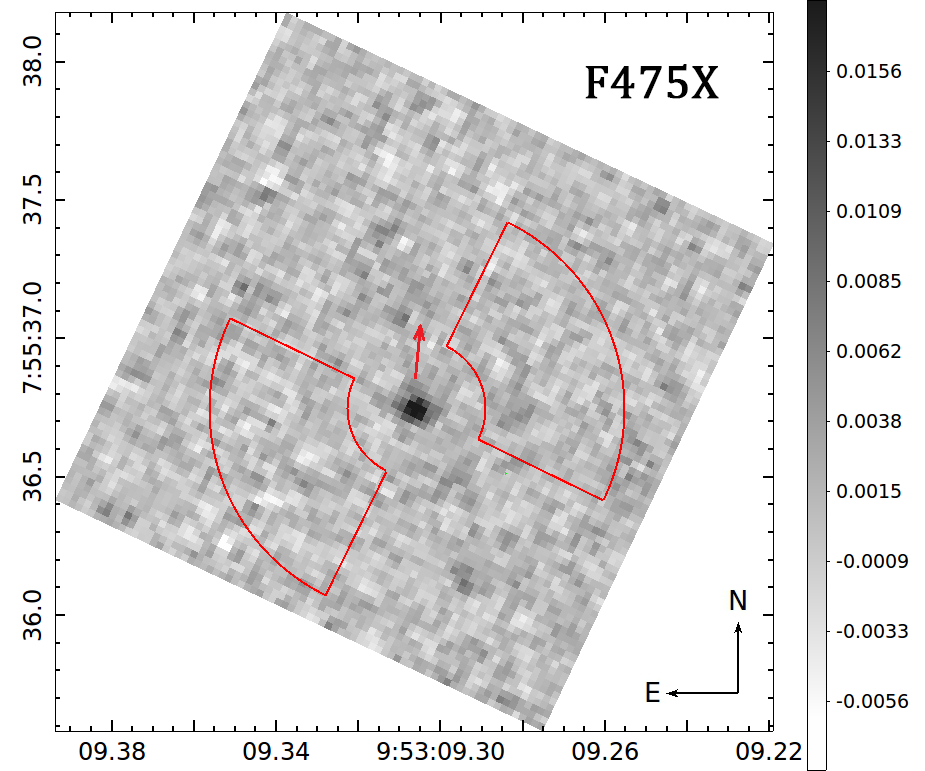
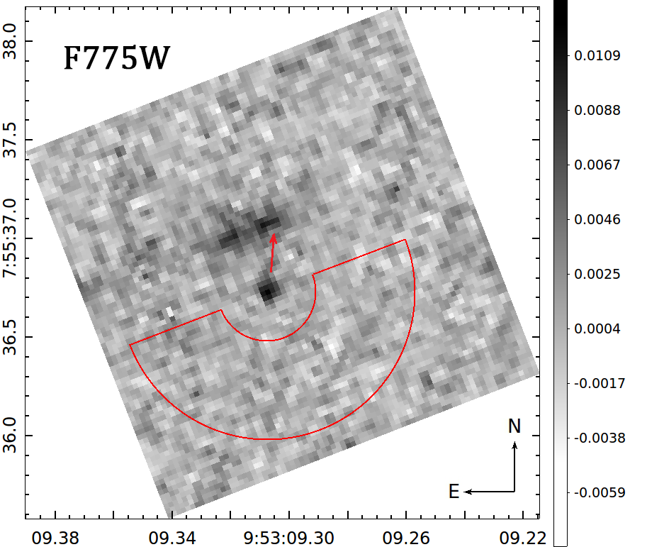
Figure 1: F475X and F775W images of $\approx 2^{\prime\prime}\times 2^{\prime\prime}$ pulsar vicinity, with $25\times 25$ mas² pixels. The pulsar counterpart is the point-like object at the center. The red arrow shows the direction of the pulsar’s proper motion; the tip of the arrow shows the position where the pulsar will be in 2031. Red contours show the areas in which the background was estimated. The vertical bars decode the image intensity in counts s^-1 per pixel.

Table 2: Optical and radio positions of PSR B0950$+$08 at different epochs

Visit	Epoch	RA (J2000)	Decl (J2000)	RA (J2000)	Decl (J2000)	$\Delta$RA	$\Delta$Decl
	MJD	(optical)	(optical)	(radio)	(radio)	(mas)	(mas)
	51544	$\cdots$	$\cdots$	09h53m09$\fs$3071(10)	$+$7∘55′36$\farcs$148(15)	$\cdots$	$\cdots$
1	58984	09h53m09$\fs$3049(5)	$+$7∘55′36$\farcs$761(7)	09h53m09$\fs$3040(10)	$+$7∘55′36$\farcs$748(15)	$13\pm 17$	$13\pm 17$
2	59005	09h53m09$\fs$3051(8)	$+$7∘55′36$\farcs$740(11)	09h53m09$\fs$3039(10)	$+$7∘55′36$\farcs$750(15)	$18\pm 19$	$-10\pm 19$
3	59279	09h53m09$\fs$3043(5)	$+$7∘55′36$\farcs$781(7)	09h53m09$\fs$3040(10)	$+$7∘55′36$\farcs$772(15)	$4\pm 17$	$9\pm 17$

Note. — The reference radio coordinates of the pulsar (first line) are taken from Brisken et al. (2002) The radio coordinates at the epochs of the HST observations are calculated using the best-fit values of proper motion $\mu_{\alpha}=-2.09$ mas yr^-1, $\mu_{\delta}=+29.46$ mas yr^-1, and parallax $\pi=3.82$ mas (Brisken et al., 2002). Offsets of the optical positions with respect to the radio positions are given in two last columns. The numbers in parentheses are the numerical values of the standard uncertainty (at the 68% level of confidence) referred to the corresponding last digits of the quoted result.

To precisely measure the International Celestial Reference System (ICRS) coordinates of the point source, we obtained astrometric solutions for our images using the Gaia EDR3 Catalog (Gaia Collaboration et al., 2021) and the IRAF tasks imcentroid and ccmap. In the UVIS and the first WFC fields of view we found five unsaturated cataloged stars, two of them are common to both fields, and only four catalogued stars in the second WFC field of view, three of them are common with the first WFC FOV. To calculate the coordinates of the reference stars at the epochs of the HST observations, we shifted their Gaia EDR3 positions, given at the reference epoch 2016.0, using the cataloged proper motion values. Astrometric fits yielded the root-mean-square (rms) residuals of 2.4 mas in the RA and 3.3 mas in the Decl for the F475X image, and 6.8 (4.0) mas and 4.4 (1.8) mas in the RA and Decl, respectively, for the first (second) F775W images. The rms centroiding uncertainties of the reference stars are $\lesssim$ 0.3 mas in the RA and Decl for all three images. The rms uncertainties of the Gaia positions of the reference objects do not exceed 0.5 mas in both coordinates and within each field. The proper motion corrections have rms uncertainties of 4.9 mas in the RA and 4.3 mas in the Decl for the F475X image, and 5.3 (2.3) mas and 4.8 (1.7) mas in the RA and Decl, respectively, for the first (second) F775W observations. As a result, combining all the uncertainties in quadrature, we obtain 5 mas in both coordinates for astrometric referencing uncertainties of the F475X image. We got 9 (4) mas and 7 (3) mas in the RA and Decl, respectively for referencing of the first (second) F775W images.

Using the Gaia-based astrometric solutions, we measured the ICRS coordinates of the point source. They are listed in Table 2, where the coordinate errors account for the astrometric referencing uncertainties and the source centroding uncertainties of 5 mas in the F475X image and 8 and 6 mas in the first and second F775W images, respectively. We compared them with predicted coordinates of the radio pulsar at the epochs of the HST observations, using the reference radio position and the proper motion and parallax provided by Brisken et al. (2002). As seen from Table 2, the optical-radio offsets are in the range of 4–18 mas, within their statistical uncertainties. This demonstrates the high accuracy of the Gaia-based HST astrometry and firmly confirms that the detected point source is indeed the pulsar counterpart.

In the HST images we do not see any extended emission that could be interpreted as a pulsar wind nebula (PWN). An extension of the pulsar image in the direction perpendicular to the pulsar’s trajectory, reported from the Subaru and VLT observations in the B band and suggested to be a PWN by (Zharikov et al., 2002, 2004), might be due to overlapping with a faint blue background source located $0\farcs 6$ south of the pulsar in the F475X image (i.e., 0$\farcs$2 west from the pulsar position in 2001, when the Subaru and VLT observations were taken, with seeing of 0$\farcs$7).

In the F775W image we see an extended object with a non-uniform brightness distribution, apparently a distant galaxy or a couple of galaxies, at about 0$\farcs$3–0$\farcs$5 north-northwest of the pulsar. Only a hint of it can be seen in the F475X image. This is the object O2 that Zharikov et al. (2004) detected in 2001 with the VLT in the I and R bands, when the pulsar was $0\farcs 58$ farther south. Obviously, if the pulsar were observed now with a ground-based telescope without adaptive optics, it would not be be resolved from the extended source.

3.2 Photometry

We measured the pulsar count rates in apertures of 5.6 pix (0$\farcs$14) and 5 pix (0$\farcs$125) radii in F475X and F775W filters, respectively. To determine the encircled energy fraction $\phi_{E}$ in these apertures, we measured $\phi_{E}$ as a function of aperture radius for 2 relatively bright, unsaturated stars in the F475X image and 5 stars in the F775W image. The obtained $\phi_{E}=0.80$ and 0.73, respectively, are close to their nominal values for these detectors for the chosen aperture sizes.

In both the F475X and F775W fields we measured the background in parts of annuli with 10 pix (0$\farcs$25) and 30 pix (0$\farcs$75) inner and outer radii (see Figure 1). In the F475X image we extracted background counts from two $90^{\circ}$ segments east and west of the pulsar to avoid an apparent background enhancements (some of them may be very faint sources) along the vertical diagonal of the square of the F475X image. In the F775W images, the background was extracted from the half-annulus (the northern half of the annulus was excluded because it contains the extended source).

Since the numbers of counts in the small pixels of the drizzled images are not statistically independent, the usual approach to noise evaluation, based on mean and standard deviation of counts (or count rates) per pixel, yields underestimated uncertainties of source count rate. Therefore, we used the “empty aperture” approach (see Section 3.4 in Skelton et al. 2014). In this approach background count rates are measured in multiple apertures of the same size as the source aperture, randomly placed within the background region. The mean $\overline{C}_{\rm bgd}$ and the variance $\sigma_{C_{\rm bgd}}^{2}$ of count rates per aperture yield the most reliable estimates for the net source count rate and its uncertainty $\sigma_{s}$:

$$C_{s}=C_{\rm tot}-\overline{C}_{\rm bgd},\quad\quad\sigma_{s}=\left(\sigma_{C_{\rm bgd}}^{2}+C_{s}t_{\rm exp}^{-1}\right)^{1/2},$$ (1)

where $C_{\rm tot}$ is the total count rate in the source aperture, and $t_{\rm exp}$ is the exposure time. Notice that the directly measured quantity $\sigma_{C_{\rm bgd}}^{2}$ includes all possible sources of background noise, i.e., the sky contribution as well as various instrumental and processing contributions. An advantage of this empirical approach is its simplicity and minimum of assumptions involved.

In our case, for each of the images we used a set of 1000 circular apertures with the same radii as the source apertures, $r_{\rm extr}=0\farcs 14$ and 0$\farcs$125 for the F475X and F775W images, respectively. The results for each of the 3 visits are presented in Table 3.

To convert the source count rate, corrected for the finite aperture size, into mean flux density, we used the inverse sensitivity header keyword photfnu (${\cal P}_{\nu}$ in Table 3) for the F475X image. For the F775W images we calculated ${\cal P}_{\nu}$, using the header keywords photflam and photplam. The resulting source fluxes are presented in first 3 lines of Table 3 for each observation.

In fourth line of Table 3 we provide photometry results for the sum of the two F775W images, aligned on the pulsar position. The pulsar’s mean flux density, $\overline{f}_{\nu}=52.9\pm 6.9$ nJy, estimated from the combined image is in excellent agreement with the weighted mean flux density, $\overline{f}_{\nu}=52.2\pm 6.8$ nJy, of the flux densities measured in the separate visits.

We see that while the F475X flux density is in good agreement with the Subaru and VLT measurements in the B band, the F775W flux is considerably lower than the I and R fluxes measured with the VLT (see Section 1 and Zharikov et al. 2004). The reason for this discrepancy is the relatively poor angular resolution of the VLT observations, which hampered correction for contamination from the nearby extended object north of the pulsar.

In Table 3, we also include FUV photometry results (Pavlov et al., 2017) corrected with account for the new ACS/SBC calibration presented by Avila et al. (2019). The lower values of the corrected inverse sensitivity ${\cal P}_{\nu}$ resulted in lower FUV flux densities than those published by Pavlov et al. (2017), by 29% and 24% for the F125LP and F140LP filters, respectively.

Table 3: Photometry of the pulsar counterpart

Filter	Visit	$t_{\rm exp}$	$r_{\rm extr}$	$\phi_{E}$	$C_{\rm tot}$	$C_{\rm bgd}$	$N_{b}$	$C_{s}$	$C_{\rm corr}$	${\cal P}_{\nu}$	$\overline{f}_{\nu}$
		(s)	(arcsec)	(%)	(cnts ks-1)	(cnts ks-1)	(cnts)	(cnts ks-1)	(cnts ks-1)	(nJy ks cnts-1)	(nJy)
F475X	1	2420	0.14	80	426	$38\pm 36$	…	$388\pm 38$	$485\pm 48$	0.123	$59.6\pm 5.9$
F775W	2	3726	0.125	73	224	$32\pm 33$	…	$192\pm 34$	$263\pm 47$	0.197	$51.8\pm 9.2$
F775W	3	2434	0.125	73	222	$22\pm 36$	…	$200\pm 38$	$274\pm 51$	0.197	$54.0\pm 10.1$
F775W	2+3	6160	0.125	73	223	$27\pm 25$	…	$196\pm 25$	$268\pm 35$	0.197	$52.9\pm 6.9$
F125LP	…	5528	0.25	66	69	…	1859	$60.8\pm 3.6$	$92.0\pm 5.4$	0.847	$77.9\pm 4.6$
F140LP	…	1774	0.25	67	35	…	642	$25.9\pm 4.5$	$39.0\pm 6.7$	1.608	$62.7\pm 10.8$

Note. — $\phi_{E}$ is the fraction of source counts in the aperture with radius $r_{\rm extr}$, $C_{\rm tot}$ is the total count rate in the source aperture, $C_{\rm bgd}=\overline{C}_{\rm bgd}\pm\sigma_{C_{\rm bgd}}$, $\overline{C}_{\rm bgd}$ and $\sigma_{C_{\rm bgd}}$ are the mean and standard deviation of background measurements, $N_{b}$ is the number of counts in the FUV background apertures, $C_{s}$ is the net source count rate, its error is estimated as $[(\sigma_{C{\rm bgd}}^{2}+C_{s}t_{\rm exp}^{-1}]^{1/2}$ for optical images and $[C_{\rm tot}t_{\rm exp}+(A_{s}/A_{b})^{2}N_{b}]^{1/2}t_{\rm exp}^{-1}$ for FUV images, where $A_{s}$ = 0.196 arcsec² and $A_{b}$ = 7.854 arcsec² are the areas of the source and background apertures (Pavlov et al., 2017), $C_{\rm corr}$ is the aperture-corrected source count rate, $\overline{f}_{\nu}=C_{\rm corr}{\cal P}_{\nu}$ is the mean flux density, and ${\cal P}_{\nu}$ is the count rate-to-flux conversion factor.

3.3 Spectral fits

Following Pavlov et al. (2017), we fit the optical-UV spectrum with the PL+BB model

$$f_{\nu}^{\rm mod}=\left[f_{\nu_{0}}\left(\frac{\nu}{\nu_{0}}\right)^{\alpha}+\frac{R_{\infty}^{2}}{d^{2}}\pi B_{\nu}(T_{\infty})\right]\times 10^{-0.4A_{\nu}},$$ (2)

where $\nu_{0}$ is the reference frequency for the PL spectrum (we chose $\nu_{0}=1\times 10^{15}$ Hz, which corresponds to $\lambda_{0}=3000$ Å), $d=262d_{262}$ pc is the distance, $T_{\infty}=T(1+z)^{-1}$ and $R_{\infty}=R(1+z)$ are the NS temperature and radius as seen by a distant observer, $z=[1-2.953(M/M_{\odot})(1\,{\rm km}/R)]^{-1/2}-1$ is the gravitational redshift, and $B_{\nu}(T_{\infty})$ is the Planck function. Below we use the notations $R_{\infty}=15R_{15}$ km and $T_{\infty}=10^{4}T_{4}$ K; at a NS mass $M=1.4M_{\odot}$, the apparent radius $R_{\infty}=15$ km corresponds to an intrinsic (circumferential) NS radius $R=12.2$ km. The extinction coefficient $A_{\nu}$ is proportional to color excess $E(B-V)$. According to Pavlov et al. (2017), the most plausible range of the color excess for B0950 is $E(B-V)=0.01$–0.03, but higher values, perhaps up to 0.06, are not excluded. We will consider the range $E(B-V)=0.01$–0.06 and use Cardelli et al. (1989) to connect $A_{\nu}$ with $E(B-V)$.

To fit the model given by Equation (2) to the measured broad-band spectrum, we vary the model parameters to minimize the following $\chi^{2}$ statistic

$$\chi^{2}=\sum_{i}\frac{\left(\overline{f}_{\nu,i}-\overline{f}_{\nu,i}^{\rm mod}\right)^{2}}{\sigma_{f_{\nu,i}}^{2}}\,,$$ (3)

where $\overline{f}_{\nu,i}$ and $\sigma_{f_{\nu,i}}$ are the mean flux density and its error in the $i$-th filter (given in the last column of Table 3),

$$\overline{f}_{\nu,i}^{\rm mod}=\left[\int f_{\nu}^{\rm mod}\nu^{-1}T_{i}(\nu)\,d\nu\right]\left[\int T_{i}(\nu)\nu^{-1}\,d\nu\right]^{-1},$$ (4)

and $T_{i}(\nu)$ is the passband throughput for the $i$-th filter as a function of frequency. In our fits we included all the HST observations available (5 filters) and the Subaru observation in the B filter as it was not contaminated by the red extended object north of the pulsar. The throughputs for the HST and Subaru B filters were taken from the SVO filter profile service.

The model given by Equation (2) has 5 parameters. Because of the few data points and a correlation between the parameters, we chose to fit 3 of them: $T_{\infty}$, $\alpha$ and $f_{\nu_{0}}$ at fixed values of $E(B-V)$ and $R_{\infty}/d=1.86\times 10^{-15}R_{15}/d_{262}$ (cf. Pavlov et al. 2017). An example of such a fit at plausible values $E(B-V)=0.02$ and $R_{15}/d_{262}=1$ is shown in Figure 2. The best-fit parameters are $T_{4}=8.0^{+0.9}_{-1.4}$, $\alpha=-0.32^{+0.29}_{-0.26}$, and $f_{\nu_{0}}=41^{+8}_{-7}$ nJy. With the reduced $\chi_{\rm min}^{2}=1.46$ for 3 degrees of freedom, the fit is not perfect (perhaps because there are systematic errors unaccounted for), but it is substantially better than the fit obtained by Pavlov et al. (2017), with the reduced $\chi_{\rm min}^{2}=3.8$ for 4 degrees of freedom (for $E(B-V)=0.02$, $R_{15}/d_{262}=0.8$).

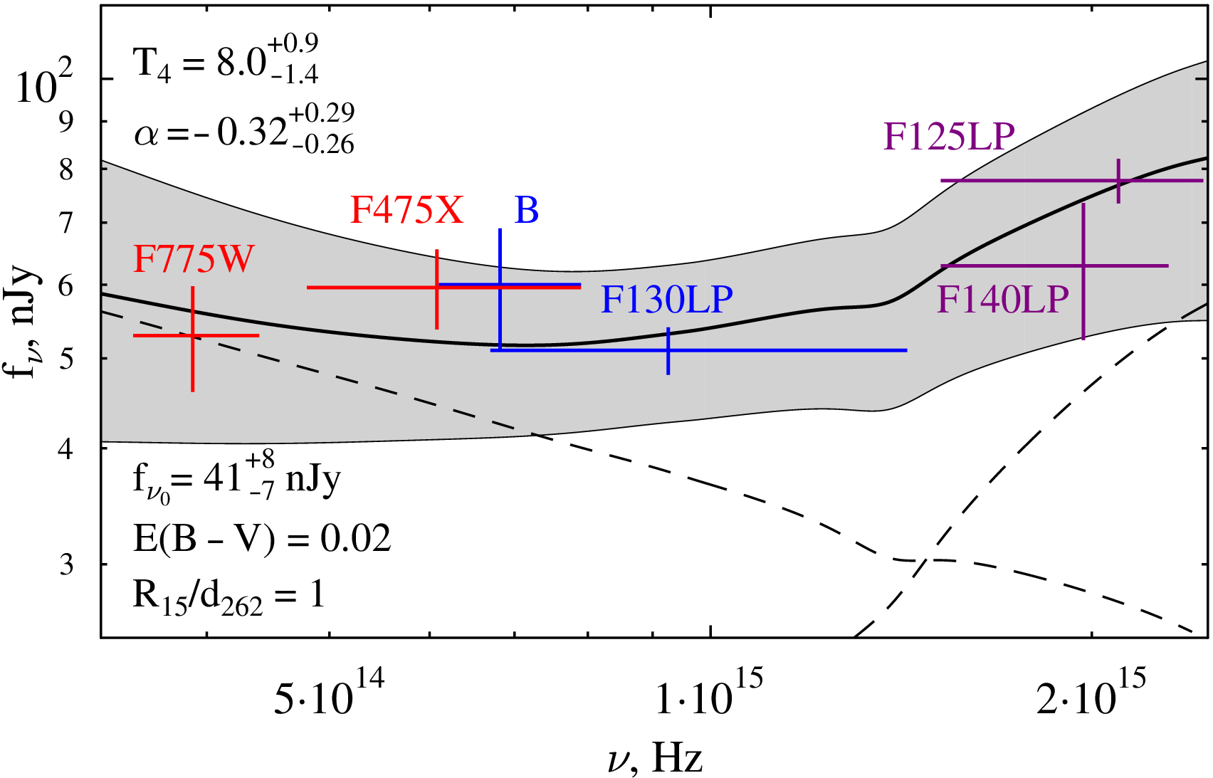
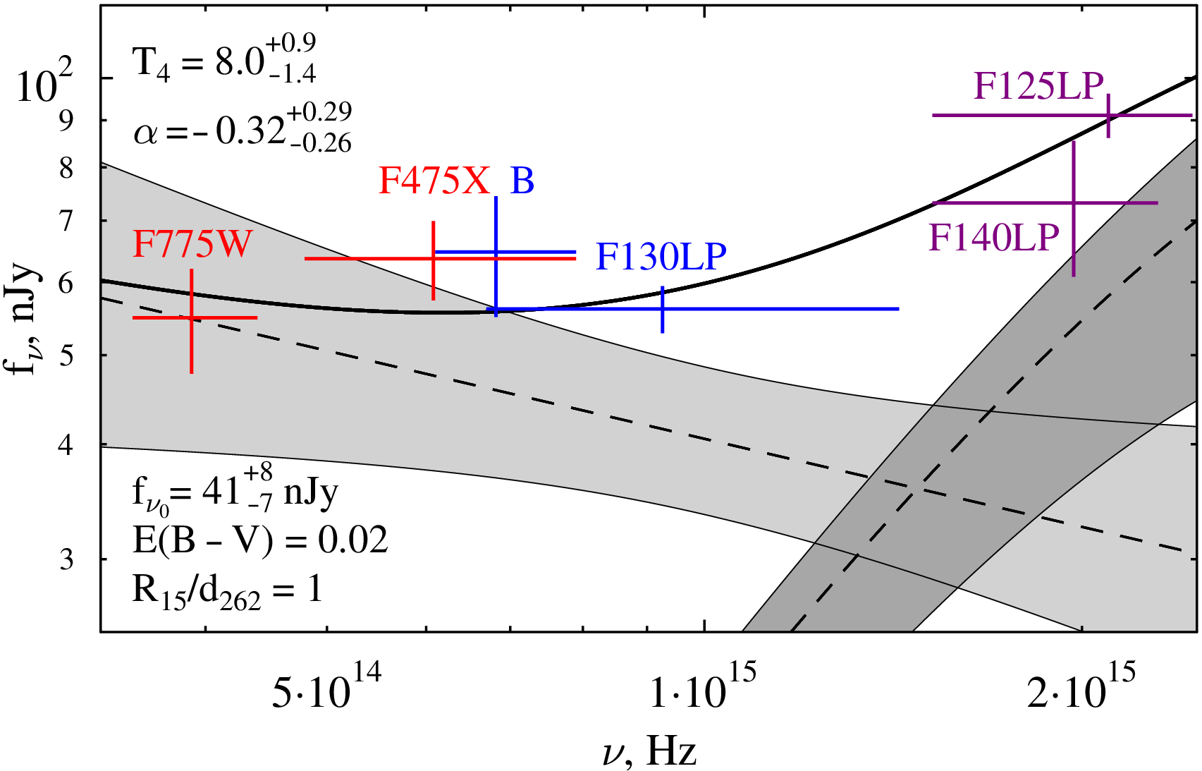
Figure 2: Observed (left) and dereddenned (right) optical-UV spectra of the pulsar counterpart. The thick solid lines show the best fit for the HST and Subaru (B) data with the PL+BB model at fixed $E(B-V)=0.02$ and $R_{15}/d_{262}=1$. The dashed lines show the best-fit spectra of the PL and BB components. The shaded areas demonstrate fit uncertainties, at the 68% confidence level, for the components (right panel) and their sum (left panel).

For the direct comparison with Pavlov et al. (2017), we also fit the model with $R_{15}/d_{262}=0.8$. Although the best-fit optical-FUV spectrum (reduced $\chi^{2}_{\rm min}=1.39$) is qualitatively similar to that shown in Figure 3 of Pavlov et al. (2017), the fitting parameters are quite different: $T_{4}=10.1^{+1.5}_{-2.0}$, $\alpha=-0.28^{+0.28}_{-0.26}$ versus $T_{4}=16.8\pm 2.6$, $\alpha=-1.17\pm 0.43$. The lower temperature and more gradual slope of of the PL component are caused by lower values for the FUV flux due to the corrected calibration of the ACS/SBC sensitivity, and by the lower optical flux, which is not distorted by a contribution from the nearby extended source, unlike the previous ground-based observations in red filters.

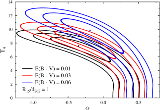
Figure 3: Confidence contours in the $\alpha$–$T_{\infty}$ plane for $R_{15}/d_{262}=1$ and $E(B-V)=0.01$, 0.03 and 0.06 (black, red and blue lines, respectively). The contours are plotted for the 68.3 %, 95.5 % and 99.7 % confidence levels (for two parameters of interest). The third parameter $f_{\rm\nu_{0}}$ was varied to minimize $\chi^{2}$ at each point of the $\alpha$–$T_{\infty}$ plane.

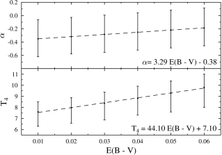
Figure 4: Dependencies of the main fitting parameters on color excess for $R_{15}/d_{262}=1$. The uncertainties are at the 68% confidence level. The equations in the panels are linear approximations of the dependencies.

The uncertainties of the fitting parameters grow with raising the confidence level. Moreover, the lower bound on temperature tends to zero at a sufficiently high confidence level. For instance, in the above-considered example of $E(B-V)=0.02$, $R_{15}/d_{262}=1$, we obtain $T_{4}=8.0^{+1.4}_{-2.8}$ at the 90% confidence, but $T_{4}=8.0^{+2.0}_{-8.0}$ at the 99% confidence. This behavior is illustrated in Figure 3, which shows 68.3%, 95.5% and 99.7% confidence contours (for two parameters of interest) for $R_{15}/d_{262}=1$, and three values of color index: $E(B-V)=0.01$, 0.03, and 0.06. We see that at $T_{4}\lesssim 2$–3 the fits become insensitive to the temperature value, and the high-confidence contours fall down to zero temperature, for all the considered color indices.

Figure 3 also shows that both $T_{\infty}$ and $\alpha$ grow with increasing $E(B-V)$. The temperature is strongly (anti)correlated with the PL slope, which means that the temperature uncertainty could be reduced significantly if optical (and IR) fluxes were measured more precisely, with additional filters.

The dependencies of the temperature and spectral slope on color index are shown in Figure 4. At $E(B-V)<0.06$ they can be approximated by linear functions given in the figure panels. The fitting parameters also depend on the $R_{15}/d_{262}$ parameter; in particular, the temperature is proportional to $(R_{15}/d_{262})^{-1.5}$ (Pavlov et al., 2017).

Although the probability of very low (undetectable) temperatures is low, such temperatures are not firmly excluded by the current data. Therefore we fit the same data points with a one-component absorbed PL model. For $E(B-V)=0.02$, we obtained $\alpha=+0.36\pm 0.06$, $f_{\nu_{0}}=66.7\pm 2.3$ nJy, reduced $\chi_{\rm min}^{2}=1.97$ for 4 degrees of freedom. According to the F-test, adding the BB to the PL component better describes the data with a probability of 0.78.

Combining the uncertainties of extinction and radius-to-distance ratio broadens the range of plausible BB temperatures. For instance, for $0.8\leqslant R_{15}/d_{262}\leqslant 1.1$ and $0.01\leqslant E(B-V)\leqslant 0.03$, we obtained $5.8<T_{4}<12.3$ at the 68% confidence level, and $4.7<T_{4}<13.1$, at the 90% confidence level. The most conservative temperature upper bound, for $R_{15}/d_{262}=0.8$ and $E(B-V)=0.06$, is $T_{4}<17$, at the 99% confidence level.

4 Discussion

Thanks to the exquisite angular resolution of the HST, we were able to resolve the pulsar counterpart from the close-by red galaxy and accurately measure its optical fluxes. We found that the flux in the F775W filter (pivot wavelength 7693 Å) is a factor of about 1.5 (1.7) lower than the $I$ ($R$) fluxes previously measured with the VLT with a much worse angular resolution. The reduced flux density in the red part of the spectrum and the higher FUV sensitivity inferred from the recent recalibration of the ACS/SBC detector lead to a more gradual slope of the PL component and a lower temperature of the BB component, in the PL + BB fit of the optical-FUV spectrum. In particular, the best-fit temperature is a factor of 1.5–2 lower than the previous estimates by Pavlov et al. (2017). For plausible ranges of color index and radius-to-distance ratio, the gravitationally redshifted temperature is in the range $5\lesssim T_{\infty}/10^{4}\,{\rm K}\lesssim 13$ (at the 90% confidence), with a most likely value $T_{\infty}\sim 8\times 10^{4}$ K. The corresponding non-redshifted temperatures are a factor of $1+z=[1-0.246(M/M_{\odot})(12\,{\rm km}/R)]^{-1/2}$ higher; for instance, $6\lesssim T/10^{4}\,{\rm K}\lesssim 16$ for $M=1.4M_{\odot}$ and $R=12$ km.

Such temperatures are much higher than predicted by models of passive cooling of NSs at ages $\gtrsim 10$ Myr. If the real age of B0950 is close to its spin-down age of 17.5 Myr, this requires heating processes to operate in its interiors. According to Gonzalez & Reisenegger (2010), the most plausible heating mechanism for an ordinary (nonrecycled) pulsar with a strong magnetic field is the so-called vortex creep (or frictional) heating caused by interaction of vortex lines of the faster rotating neutron superfluid with the slower rotating normal matter in the inner NS crust. The estimated temperature range is generally consistent with the NS thermal evolution with allowance for the vortex creep heating, for either direct or modified Urca cooling (see the lower panels in Figures 4 and 5 in Gonzalez & Reisenegger (2010) and the upper panel in Figure 5 in Guillot et al. (2019)).

However, the true age of a pulsar can be different from the spin-down age. For instance, using the Bayesian approach, Igoshev (2019) estimated a most probable kinematic age of B0950 to be as small as $\approx 2$ Myr, with a 95% credible interval of 0.4–17 Myr. The upper bound of this interval is close to the spin-down age, requiring the internal heating of the NS, as discussed above. Within this very wide interval the agreement between the derived surface temperature and the predictions of passive NS cooling scenarios is only possible for ages $\lesssim$ 4 Myr (see Figure 7 in Igoshev 2019). According to Igoshev (2019), such small ages could be due to a fast decay of the NS magnetic field, at a timescale of $\lesssim 5$ Myr, and/or a large initial spin period of the pulsar, comparable with its current value. Such explanations imply that B0950 is a very peculiar object among other old ordinary pulsars. The required decay timescale is significantly shorter than the Ohmic dissipation timescale of $\gtrsim 10$ Myr caused by lattice impurities of the nuclear crystal in the NS crust (see Igoshev et al. 2021 for a recent review of NS magnetic field evolution). Recent 2D and 3D simulations of magneto-thermal evolution of NSs, performed mainly for super-strong magnetic fields $B\sim 10^{14}-10^{15}$ G typical for magnetars, show that short timescales are possible if the non-linear Hall effect is taken into account and the presence of super-strong toroidal field component inside the crust is assumed (e.g., Geppert & Viganò, 2014; Gourgouliatos & Hollerbach, 2018). These models allow one to explain some observational properties of magnetars. However, B0950 does not show any magnetar properties such as hard X-ray or soft gamma-ray flares. There are also no signs of the presence of large hot spots on its surface typical for magnetars. Its surface magnetic field is within the range of $\sim 10^{11}-10^{12}$ G, typical for ordinary pulsars. The assumption of a long initial period, close to the current period of 253 ms, looks rather arbitrary, and it is hardly consistent with much shorter periods of young ordinary pulsars. These contradictions do not exclude the possibility of B0950 being younger than its spin-down age, but such a large difference in ages appears to be unlikely as the observed properties B0950 are not substantially different from those of other members of the old pulsar class.

In addition, the small value of the most probable kinematic age of B0950, estimated by Igoshev (2019), is mostly due to the unusually small transverse velocity of this pulsar, which requires a large radial velocity at the assumed probability distribution of total velocities of pulsars. However, we cannot exclude the possibility that the actual total and radial velocities of B0950 are substantially smaller than the most probable values.

It would be useful to perform 3D magneto-thermal evolution simulations with allowance for the Hall effect for the field range typical for ordinary pulsars and estimate the timescale of their field decay. As the Hall drift timescale is $\propto B^{-1}$ (e.g., Igoshev et al., 2021), one can expect a 2-3 orders of magnitude longer drift timescale for an ordinary pulsar than for a magnetar, comparable to the Ohmic field decay time scale, in which case we do not expect a large hot spot on the NS surface to form. On the other hand, simple estimates (e.g., Gonzalez & Reisenegger, 2010) show that in order to heat B0950 by the magnetic field dissipation to the temperatures inferred from our observations, its magnetic field should be $\sim 10^{13}$ G, much higher than the spin-down value of $2.4\times 10^{11}$ G.

To estimate the parameters that determine the rate of the vortex creep heating (such as the so-called “excess angular momentum” – see, e.g., Gügercinoğlu 2017 for a recent discussion), more pulsars with ages $\gtrsim$ a few Myr should be observed in the FUV-optical range to estimate the NS temperatures and understand the thermal evolution of old NSs. Until new space observatories with UV capabilities are launched, such observation are only possible with the HST.

The spectral slope of the PL component found from the HST observations, $\alpha=-0.3\pm 0.3$, is not nearly as steep as $\alpha=-1.2\pm 0.4$ based on the previous ground-based observations. The newly measured slope is within the range of $-1\lesssim\alpha\lesssim 0$, found for the optical spectra of other rotation-powered pulsars (e.g., Mignani et al. 2007). The optical PL slope of B0950 is flatter than in the X-ray range – e.g., $\alpha_{X}=-0.75\pm 0.15$ for a single-component PL fit (Zavlin & Pavlov, 2004), which implies a spectral break between the optical and X-rays, similar to other pulsars investigated in both ranges. However, the break disappears if the thermal component from pulsar hot polar caps heated by relativistic particles from the pulsar magnetosphere contributes to X-ray emission, leading to $\alpha_{X}=-0.3\pm 0.1$, which is consistent with the optical slope. It is thus unclear whether or not the optical and X-ray nonthermal photons are produced by the same emission mechanism and the same relativistic particle distribution in the pulsar magnetosphere. The properties of the polar caps and their contribution to the X-ray spectrum can be inferred from timing and spectral analysis of deeper X-ray observations.

Although it is quite plausible that the FUV flux of B0950 is dominated by the thermal component, we cannot firmly exclude the possibility of the temperature being lower, and the spectral index $\alpha$ larger, than estimated above (see Figure 3). In other words, if we choose a high confidence level for the fit parameter uncertainties, we can only put an upper limit on the brightness temperature. For instance, at the confidence level of 99%, we obtained $T_{\infty}<1.0\times 10^{5}$ K at $E(B-V)=0.02$ and $R_{15}/d_{262}=1$, and $T_{\infty}<1.7\times 10^{5}$ K at $E(B-V)=0.06$ and $R_{15}/d_{262}=0.8$. Given the dependencies of $T_{\infty}$ on $E(B-V)$ and $R_{\infty}/d$ (see Section 3.3), the value $T_{\infty}=1.7\times 10^{5}$ K can be considered as the most conservative upper limit on the temperature.

Because of the $\alpha$-$T_{\infty}$ anti-correlation (see Figure 3), very low temperature values correspond to positive values of $\alpha$, i.e., the flux density increasing with frequency (e.g., $\alpha=+0.36\pm 0.06$ at $E(B-V)=0.02$). Not only the low-temperature solutions are less acceptable statistically, but also none of the pulsars with a measured slope of the optical PL component shows so large $\alpha$; the only pulsar with a positive (but smaller) $\alpha$ is the Crab pulsar, with $\alpha=0.16\pm 0.07$ (Sollerman et al., 2019). This can be considered as an additional argument in favor of the presence of the thermal UV component in the B0950 spectrum.

To conclude, our observations of B0950 with the HST support the presence of the thermal UV component, whose temperature, however, is lower than previously suggested. They have also shown that the slope of the nonthermal spectral component, presumably emitted from the pulsar magnetosphere, is not as steep as found from groundbased observations. To firmly prove the presence of the hot thermal emission and measure the temperature and PL slope more precisely, deep HST and/or JWST observation in several IR-optical-UV filters are needed. To study the thermal and magnetospheric evolution of NSs, it would be very important to observe a large sample of isolated NSs of various types, employing the unique UV capabilities of the HST.

References

- Alpar et al. (1984) Alpar, M. A., Pines, D., Anderson, P. W., & Shaham, J. 1984, ApJ, 276, 325, doi: 10.1086/161616
- Avila et al. (2019) Avila, R. J., Bohlin, R., Hathi, N., et al. 2019, SBC Absolute Flux Calibration, Tech. rep.
- Brisken et al. (2002) Brisken, W. F., Benson, J. M., Goss, W. M., & Thorsett, S. E. 2002, ApJ, 571, 906, doi: 10.1086/340098
- Cardelli et al. (1989) Cardelli, J. A., Clayton, G. C., & Mathis, J. S. 1989, ApJ, 345, 245, doi: 10.1086/167900
- Casertano et al. (2000) Casertano, S., de Mello, D., Dickinson, M., et al. 2000, AJ, 120, 2747, doi: 10.1086/316851
- Deustua et al. (2017) Deustua, S. E., Mack, J., Bajaj, V., & Khandrika, H. 2017, WFC3/UVIS Updated 2017 Chip-Dependent Inverse Sensitivity Values, Space Telescope WFC Instrument Science Report
- Gaia Collaboration et al. (2021) Gaia Collaboration, Brown, A. G. A., Vallenari, A., et al. 2021, A&A, 649, A1, doi: 10.1051/0004-6361/202039657
- Geppert & Viganò (2014) Geppert, U., & Viganò, D. 2014, MNRAS, 444, 3198, doi: 10.1093/mnras/stu1675
- Gonzalez & Reisenegger (2010) Gonzalez, D., & Reisenegger, A. 2010, A&A, 522, A16, doi: 10.1051/0004-6361/201015084
- Gourgouliatos & Hollerbach (2018) Gourgouliatos, K. N., & Hollerbach, R. 2018, ApJ, 852, 21, doi: 10.3847/1538-4357/aa9d93
- Gügercinoğlu (2017) Gügercinoğlu, E. 2017, MNRAS, 469, 2313, doi: 10.1093/mnras/stx985
- Guillot et al. (2019) Guillot, S., Pavlov, G. G., Reyes, C., et al. 2019, ApJ, 874, 175, doi: 10.3847/1538-4357/ab0f38
- Hack et al. (2013) Hack, W. J., Dencheva, N., & Fruchter, A. S. 2013, in Astronomical Society of the Pacific Conference Series, Vol. 475, Astronomical Data Analysis Software and Systems XXII, ed. D. N. Friedel, 49
- Igoshev (2019) Igoshev, A. P. 2019, MNRAS, 482, 3415, doi: 10.1093/mnras/sty2945
- Igoshev et al. (2021) Igoshev, A. P., Popov, S. B., & Hollerbach, R. 2021, Universe, 7, 351, doi: 10.3390/universe7090351
- Larson & Link (1999) Larson, M. B., & Link, B. 1999, ApJ, 521, 271, doi: 10.1086/307532
- Manchester et al. (2005) Manchester, R. N., Hobbs, G. B., Teoh, A., & Hobbs, M. 2005, VizieR Online Data Catalog, VII/245
- Merline & Howell (1995) Merline, W. J., & Howell, S. B. 1995, Experimental Astronomy, 6, 163, doi: 10.1007/BF00421131
- Mignani et al. (2007) Mignani, R. P., Zharikov, S., & Caraveo, P. A. 2007, A&A, 473, 891, doi: 10.1051/0004-6361:20077774
- Page et al. (2009) Page, D., Lattimer, J. M., Prakash, M., & Steiner, A. W. 2009, ApJ, 707, 1131, doi: 10.1088/0004-637X/707/2/1131
- Pavlov (1992) Pavlov, G. G. 1992, in IAU Colloq. 128: Magnetospheric Structure and Emission Mechanics of Radio Pulsars, ed. T. H. Hankins, J. M. Rankin, & J. A. Gil, 220
- Pavlov et al. (2017) Pavlov, G. G., Rangelov, B., Kargaltsev, O., et al. 2017, ApJ, 850, 79, doi: 10.3847/1538-4357/aa947c
- Pavlov et al. (1996) Pavlov, G. G., Stringfellow, G. S., & Cordova, F. A. 1996, ApJ, 467, 370, doi: 10.1086/177612
- Pilkington et al. (1968) Pilkington, J. D. H., Hewish, A., Bell, S. J., & Cole, T. W. 1968, Nature, 218, 126, doi: 10.1038/218126a0
- Shibazaki & Lamb (1989) Shibazaki, N., & Lamb, F. K. 1989, ApJ, 346, 808, doi: 10.1086/168062
- Skelton et al. (2014) Skelton, R. E., Whitaker, K. E., Momcheva, I. G., et al. 2014, ApJS, 214, 24, doi: 10.1088/0067-0049/214/2/24
- Sollerman et al. (2019) Sollerman, J., Selsing, J., Vreeswijk, P. M., Lundqvist, P., & Nyholm, A. 2019, A&A, 629, A140, doi: 10.1051/0004-6361/201935086
- Tody (1986) Tody, D. 1986, in Society of Photo-Optical Instrumentation Engineers (SPIE) Conference Series, Vol. 627, Instrumentation in astronomy VI, ed. D. L. Crawford, 733, doi: 10.1117/12.968154
- Tody (1993) Tody, D. 1993, in Astronomical Society of the Pacific Conference Series, Vol. 52, Astronomical Data Analysis Software and Systems II, ed. R. J. Hanisch, R. J. V. Brissenden, & J. Barnes, 173
- Yakovlev & Pethick (2004) Yakovlev, D. G., & Pethick, C. J. 2004, ARA&A, 42, 169, doi: 10.1146/annurev.astro.42.053102.134013
- Zavlin & Pavlov (2004) Zavlin, V. E., & Pavlov, G. G. 2004, ApJ, 616, 452, doi: 10.1086/424894
- Zharikov et al. (2004) Zharikov, S. V., Shibanov, Y. A., Mennickent, R. E., et al. 2004, A&A, 417, 1017, doi: 10.1051/0004-6361:20034230
- Zharikov et al. (2002) Zharikov, S. V., Shibanov, Y. A., Koptsevich, A. B., et al. 2002, A&A, 394, 633, doi: 10.1051/0004-6361:20021155