LibSC: Library for Scaling Correction Methods in Density Functional Theory

Abstract

In recent years, a series of scaling correction (SC) methods have been developed in the Yang laboratory to reduce and eliminate the delocalization error, which is an intrinsic and systematic error existing in conventional density functional approximations (DFAs) within density functional theory (DFT). Based on extensive numerical results, the SC methods have been demonstrated to be capable of reducing the delocalization error effectively and producing accurate descriptions for many critical and challenging problems, including the fundamental gap, photoemission spectroscopy, charge transfer excitations and polarizability. In the development of SC methods, the SC methods were mainly implemented in the QM4D package that was developed in the Yang laboratory for research development. The heavy dependency on the QM4D package hinders the SC methods from access by researchers for broad applications. In this work, we developed a reliable and efficient implementation , LibSC for the global scaling correction (GSC) method and the localized orbital scaling correction (LOSC) method. LibSC will serve as a light-weight and open-source library that can be easily accessed by the quantum chemistry community. The implementation of LibSC is carefully modularized to provide the essential functionalities for conducting calculations of the SC methods. In addition, LibSC provides simple and consistent interfaces to support multiple popular programing languages, including C, C++ and Python. In addition to the development of the library, we also integrated LibSC with two popular and open-source quantum chemistry packages, the Psi4 package and the PySCF package, which provides immediate access for general users to perform calculations with SC methods.

Department of Physics, Duke University, Durham, North Carolina 27708, USA numbers=left, stepnumber=1, numberstyle=, numbersep=10pt

1 Introduction

Density functional theory (DFT) ^{1, 2, 3} has been widely used nowadays to describe the electron structure of matters in chemistry, physics and materials science. In the pursuit of accurate predictions from theoretical simulations based on DFT, developing accurate density functional approximations (DFAs) within DFT has become an active research field in quantum chemistry and condensed matter physics. During the last decades, conventional DFAs, including the local density approximations (LDAs) ^{4, 5}, generalized gradient approximations (GGAs) ^{6, 7, 8} and hybrid functionals ^{9, 7, 10, 11, 12}, have achieved great success. However, conventional DFAs involve the intrinsic and systematic delocalization error ^{13, 14, 15, 16}, which is the underlying challenge for many critical applications ^{17, 18, 19, 20, 21, 15, 13, 16, 22}.

To reduce the systematic delocalization error, many approaches have been developed, including range-separated functionals ^{23, 24, 25, 26, 27, 28, 29}, self-interaction error corrected functionals^{30, 19, 31, 32, 33, 34, 35, 36}, Koopmans-compliant functionals, ^{37, 38} and generalized transition state methods ³⁹ and related developments ⁴⁰.

In addition to these aforementioned approaches, a series of scaling correction (SC) methods ^{41, 42, 43, 44, 45, 46}, including the global scaling correction (GSC) ^{41, 46}, the local scaling correction (LSC) ⁴² and the localized orbital scaling correction (LOSC) ^{43, 44, 45} methods, have been developed in the Yang laboratory to tackle the delocalization error in conventional DFAs. With extensive numerical results ^{41, 42, 43, 43, 47, 48, 49, 50, 51}, these SC methods have been demonstrated to be capable of reducing the delocalization error effectively and producing accurate descriptions for many critical and challenging problems, including the fundamental gap ^{41, 43, 47}, photoemission spectroscopy ^{43, 47, 50}, photoexcitation energies ^{47, 48, 49} and polarizability ^{42, 51}. Therefore, a reliable and stable implementation for the SC methods can be very beneficial and meaningful to the electronic structure theory community, which helps to promote DFT with commonly used DFAs and with the SC methods for broader applications.

However, along the development of SC methods, the implementation was mainly developed in the QM4D package ⁵², which is an in-house quantum chemistry package in the Yang laboratory for research development. In this work, we developed a reliable and stable implementation for the GSC and LOSC methods in LibSC, which will serve as a light-weight and open-source library to provide the essential functionalities for conducting calculations of the SC methods. With the simple and consistent interface to support multiple popular programing languages, including C, C++ and Python, we aim to provide future LibSC users great flexibility to implement the SC methods in different quantum chemistry packages of their choices in a short development cycle. In addition to the development of the library, we also integrated LibSC with two popular and open-source quantum chemistry packages, the Psi4 package ⁵³ and the PySCF package ⁵⁴, which provides immediate access for researchers to perform calculations of SC methods easily. We will describe the philosophy and methodology of the design for LibSC and show its applications.

2 Theoretical Background

We start with a brief review for the key concept of the delocalization error ^{13, 14, 15, 16}, which is the central problem that the SC methods are designed to solve. The delocalization error characterizes the incorrect behavior of conventional DFAs compared to the exact functional in DFT, and it can be understood from the perspective of systems with fractional number of electrons. According to the Perdew-Parr-Levy-Balduz (PPLB) condition ^{55, 56, 57}, the exact total energy $E(N)$, as a function of electron number, should be piecewise linear between any two adjacent integer points. Critically, the manifestation of the delocalization error has been shown to be size-dependent ¹³. For small systems, conventional DFAs usually well predict total energies for integer systems. However, conventional DFAs severely underestimate the total energies for fractional systems ^{13, 14}. Such underestimation from conventional DFAs leads to a convex $E(N)$ curve, which is the manifestation of the delocalization error for small systems. For large systems, the behavior is different. The deviation of the $E(N)$ from the linearity condition decreases when the size of the system becomes larger, and vanishes at the bulk limit ¹³. However, the delocalization error manifests as the underestimation for the total energies of integer systems with the addition or removal of an electron, which produces the $E(N)$ curve with wrong slopes at the bulk limit ¹³. The direct consequence for the delocalization error is the large error in the prediction of chemical potentials, which are first derivatives of the total energy with respect to the electron number, $\frac{\partial E}{\partial N}\Big{|}_{\pm}$ from the two sides of the integer $N$. The chemical potentials $\frac{\partial E}{\partial N}\Big{|}_{-}$ and $\frac{\partial E}{\partial N}\Big{|}_{+}$ have been rigorously proved to be the energy of the highest occupied molecular orbital (HOMO) and the energy of the lowest unoccupied molecular orbital (LUMO) respectively ¹⁴ within the Kohn-Sham DFT, in which the approximate exchange-correction energy is an explicit functional of electron density, or the generalized Kohn-Sham DFT, in which the approximate exchange-correction energy is an explicit functional of the first-order density matrix. Therefore, when the PPLB condition ⁵⁵ is satisfied, HOMO and LUMO energies connect the first ionization potential (IP) and the first electron affinity (EA) ¹⁴, which read

$$\epsilon_{{\rm{HOMO}}} =\frac{\partial E}{\partial N}\Big{|}_{-}=E(N)-E(N-1)=-{\rm{IP},}$$ (1)

$$\epsilon_{{\rm{LUMO}}} =\frac{\partial E}{\partial N}\Big{|}_{+}=E(N+1)-E(N)=-{\rm{EA}.}$$ (2)

According to Eqs. 1 and 2, the direct results of the delocalization error are the underestimation of the first IP from the HOMO energy and the overestimation of the first EA from the LUMO energy, thus the drastic underestimation of the fundamental gap from the HOMO-LUMO energy gap ¹⁴.

To reduce the delocalization error, the SC methods impose the PPLB condition to associated DFAs either “globally” or “locally” to construct total energy corrections and restore the linear behavior between integers. Specifically, the global scaling correction (GSC) method ⁴¹ imposes the PPLB condition globally through the canonical orbitals and their occupation numbers. Within the GSC, the total energies of integer systems remain the same as those from the parent DFA. The energy correction from the GSC is constructed as the energy compensation to the corresponding linear interpolation and it is effective for fractional systems only, which is expressed as an addition to the total energy

$$\Delta_{{\rm{GSC}}}(N+n)=(1-n)E(N)+nE(N+1)-E(N+n).$$ (3)

Based on Eq. 3, the energy correction for GSC at the second order is given as

$$\Delta_{{\rm{GSC}}}=\frac{1}{2}\sum_{p\sigma}\kappa_{p\sigma}(n_{p\sigma}-n_{p\sigma}^{2}),$$ (4)

in which $n_{p\sigma}$ is the canonical orbital occupation number. Note that the original consideration of HOMO and LUMO ⁴¹ has been generalized to all the orbitals ^{50, 46}. The coefficient $\kappa_{p\sigma}$ in the original work of GSC ⁴¹ is approximated explicitly as

$$\kappa_{p\sigma}=\int\frac{\rho_{p\sigma}(\mathbf{r})\rho_{p\sigma}(\mathbf{r^{\prime}})}{|\mathbf{r}-\mathbf{r^{\prime}}|}\mathop{}\!\text{d}\mathbf{r}\mathop{}\!\text{d}\mathbf{r^{\prime}}-\frac{2\tau C_{\text{x}}}{3}\int\big{[}\rho_{p\sigma}(\mathbf{r})\big{]}^{\frac{4}{3}}\mathop{}\!\text{d}\mathbf{r},$$ (5)

in which the first term is the Coulomb interaction, and the second term is attributed to the Slater exchange energy. The parameters are chosen as $\tau=1$, $C_{{\rm{x}}}=\frac{3}{4}(\frac{6}{\pi})^{1/3}$, and $\rho_{p\sigma}$ is the corresponding canonical orbital density $|\psi_{p\sigma}|^{2}$. The exact coefficient $\kappa_{p\sigma}$ has been derived in a recent development of GSC (GSC2) ⁴⁶ and it is given as the second order derivative of the total energy with respect to the canonical orbital occupation number, $\kappa_{p\sigma}=\frac{\partial^{2}E}{\partial n_{p\sigma}^{2}}$, which is a completely different and more sophisticated expression compared to Eq. 5. Note that in the recent work from Xiao and coworkers ⁵⁰, they also developed GSC to involve high order relaxation of orbitals with respect to the canonical orbital occupation number and thus the energy correction goes beyond the second order expression as shown in Eq. 4. The advantage of GSC2 is that it provides exact second order corrections for any DFA ⁴⁶.

Note that the GSC preserves the total energies for integer systems and only corrects fractional systems, meaning the contribution from an orbital with an integer occupation ($n_{p\sigma}=0$ or $n_{p\sigma}=1$) is zero. Therefore, the GSC is limited to reducing the delocalization error for small and medium-sized systems. To treat the delocalization error for large systems, where the violation of the PPLB condition is no longer an issue and cannot be used as measure of the delocalization error ¹³, the local scaling correction (LSC) ⁴² method was developed later, which focuses on the local regions of the molecular system and applies the corrections locally. Combining the strategies used in GSC and LSC, the localized orbital scaling correction (LOSC) ^{43, 44, 45} was developed to provide a general approach for the systematical elimination of the delocalization error for both small and large systems. The key idea in the LOSC is to change the canonical orbitals used in GSC to the carefully designed localized orbitals, or “orbitalets”, which are one-electron orbitals that are localized both in space and in energy and are unitary combinations of both the occupied and unoccupied orbitals. The localization used in the latest version of the LOSC (called LOSC2) ⁴⁴ is defined as the minimization of the following cost function

$$F^{\sigma}=(1-\gamma)\sum_{p}\Big{(}\langle\mathbf{r}^{2}\rangle_{p\sigma}-\langle\mathbf{r}\rangle_{p\sigma}^{2}\Big{)}+\gamma C\sum_{p}\Big{(}\langle H_{\sigma}^{2}\rangle_{p\sigma}-\langle H_{\sigma}\rangle_{p\sigma}^{2}\Big{)},,$$ (6)

where

$$\langle X\rangle_{p\sigma}=\langle\phi_{p\sigma}|X|\phi_{p\sigma}\rangle,\quad X=\mathbf{r},\mathbf{r}^{2},H_{\sigma},H_{\sigma}^{2},$$ (7)

$$\phi_{p\sigma}=\sum_{q}U_{pq}^{\sigma}\psi_{q\sigma},$$ (8)

$\sigma$ is the electron spin, $\gamma$ is set to be 0.707, $C$ is set to be 1000 a.u./Å, $U_{pq}^{\sigma}$ is a unitary matrix, $\{\psi_{q\sigma}\}$ is the set of canonical orbitals, $\{\phi_{p\sigma}\}$ is the set of orbitalets, $\mathbf{r}$ is the spacial operator, and $H_{\sigma}$ is the one-electron Hamiltonian of the parent DFA. Note that we use $\psi_{i\sigma}$ and $U_{pi}^{\sigma}$ to express the dependence on the orbitalets of the localization functional $F^{\sigma}$ in Eq. 6. According to Eqs. 6-8, the orbitalets can adaptively change between the canonical orbitals and the localized orbitals, which are determined by the localization for the system of interest at the given structure. According to Eq. 8, one can apply an energy window to select COs to control the dimension of the space for localization, thus improving the computational efficiency of the localization. In practice, an energy window of [$-$30, 10] eV that covers most of the valence occupied COs and low-lying virtual COs is applied as an approximate treatment to achieve more efficient calculations.

With the application of orbitalets, the energy correction of the LOSC is generalized from the GSC to be

$$\Delta_{{\rm{LOSC}}}=\frac{1}{2}\sum_{pq\sigma}\kappa_{pq\sigma}\lambda_{pq\sigma}(\delta_{pq}-\lambda_{pq\sigma}),$$ (9)

in which $\lambda_{pq\sigma}$ is the representation of density operator under the orbitalets, namely $\lambda_{pq\sigma}=\langle\phi_{p\sigma}|\rho_{s}^{\sigma}|\phi_{q\sigma}\rangle$, and it is a matrix called the local occupation matrix. The coefficient $\kappa_{pq\sigma}$ becomes a matrix as well and is called the curvature matrix. In the original work of the LOSC (called LOSC1) ⁴³, $\kappa_{pq\sigma}$ has a similar expression to the GSC case (Eq. 5) and it is given as

$$\kappa_{pq\sigma}=\int\frac{\rho_{p\sigma}(\mathbf{r})\rho_{q\sigma}(\mathbf{r^{\prime}})}{|\mathbf{r}-\mathbf{r^{\prime}}|}\text{d}\mathbf{r}\text{d}\mathbf{r^{\prime}}-\frac{2\tau C_{x}}{3}\int[\rho_{p\sigma}(\mathbf{r})]^{\frac{2}{3}}[\rho_{q\sigma}(\mathbf{r})]^{\frac{2}{3}}\text{d}\mathbf{r},$$ (10)

in which $\rho_{p\sigma}=|\phi_{p\sigma}|^{2}$ is the density of the corresponding orbitalet. In the LOSC2 ⁴⁴, the curvature matrix is modified for better performance in molecules and given as

$$\tilde{\kappa}_{pq\sigma}=\mathrm{erf}(\xi S_{pq\sigma})\sqrt{\kappa_{pp\sigma}\kappa_{qq\sigma}}+\mathrm{erfc}(\xi S_{pq\sigma})\kappa_{pq\sigma},$$ (11)

in which $\xi=8.0$, $S_{pq\sigma}=\int\sqrt{\rho_{p\sigma}(\mathbf{r})\rho_{q\sigma}(\mathbf{r})}\mathop{}\!\text{d}\mathbf{r}$, $\mathrm{erf}(x)$ is the error function and $\mathrm{erfc}(x)$ is the complementary error function.

3 Implementation Details

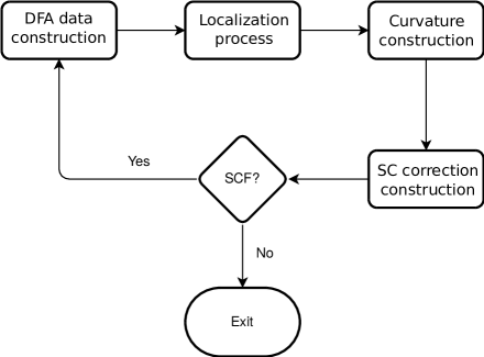
Figure 1: The flow chart of scaling correction methods.

For the development of LibSC, we focus on the implementation of GSC, LOSC1 and LOSC2 methods at the present stage. Making this choice is for three reasons: (1) these methods have been shown with much numerical success; (2) applying calculations from these three methods only requires a very low computational overhead on top of regular DFT calculations; (3) these three methods share a similar theoretical framework and analytical expressions, making their implementations easy and compact.

To illustrate the design of LibSC, we begin with the clarification for the relations and differences of these three methods in terms of implementation. First, recall the working flow of the LOSC calculations as shown in Figure 1. A general procedure for the LOSC calculation in a single self-consistent field (SCF) cycle includes three steps: (1) conducting the localization; (2) constructing the curvature matrix; (3) evaluating the corrections to the total energy and the generalized KS Hamiltonian. The way of conducting steps (1) and (2), namely, the way of generating orbitalets and constructing the curvature matrix, differentiates the different versions of the LOSC. So far, two versions of LOSC, LOSC1 ⁴³ and LOSC2 ⁴⁴, distinguish both in the localization procedure and the curvature definition. From LOSC1 to LOSC2, both the localization and the curvature matrices are improved to achieve better performance in preserving the orbitalet symmetry and degeneracy. Accordingly, the localization and curvature used in LOSC1 are called localization1 and curvature1. Similar names localization2 and curvature2 are applied to LOSC2. Second, we clarify the connections between the LOSC and the GSC. To be clear, the GSC ⁴¹ is a special case in the framework of LOSC (for both LOSC1 and LOSC2), in which the localization does not take place, yielding orbitalets that are just canonical orbitals and the curvature matrix is equivalent to the one defined in Eq. 5. Therefore, the general implementation of LOSC would cover the GSC method with the localization turned off. To make a clear illustration, we show the relations and comparisons between GSC, LOSC1 and LOSC2 in Table 1. Only bolded methods in the table are supported in LibSC.

Table 1: Options in the GSC, LOSC1, LOSC2 method and the support from LibSC.

	curvature0	curvature1	curvature2
no localization	GSC (v0)41	GSC (v1)	GSC (v2)
localization1	N/A	L1C1 (LOSC1) 43	N/A
localization2	N/A	L2C1	L2C2 (LOSC2)44
*The bolded methods are supported in LibSC.

Based on the workflow of LOSC and GSC calculations shown in Figure 1, we designed LibSC as a collection of three modules, namely, the localization module, the curvature matrix module and the correction construction module, to provide the essential functionalities for LOSC and GSC calculations. As the LOSC is a generalized case that covers the case of the GSC, the implementation of LibSC is based on the expressions from the LOSC. For the localization module, LibSC currently supports only the localization2 ⁴⁴. The Jacob-Sweep algorithm ⁵⁸ was implemented to perform the optimization problem for the localization (see the Supporting Information for details). For the curvature module, LibSC supports three versions, curvature0 ⁴¹, curvature1 ⁴³ and curvature2 ⁴⁴. curvature0 is a special case of curvature1 and can be called in LibSC by setting the curvature version to 1 and changing the default parameter $\tau$ to 1.00. Density fitting ^{59, 60} is used to evaluate the Coulomb interaction contribution in the curvature matrix for better efficiency (see the first term in Eq. 10 for example). For the correction construction module, the implementation is straightforward and based on the analytical expressions (see Eq. 9).

For the details of implementation, we summarize the design choices in the following:

• Languages: LibSC supports three programing languages, namely C++, C and Python. The core of LibSC that provides all the key functionalities of LOSC and GSC methods is implemented with morden C++11 for the consideration of computational efficiency. The C++ core of the library is bridged with C and Python programing languages to provide corresponding interfaces and avoid code duplications.

• Style: The object-oriented programming (OOP) technique is used to in the localization module and curvature module to deal with different versions and avoid code duplications. The functional programming is used in the correction module and the C code.

• Data Structure: The main data structure in the library is the matrix object, which is represented by the MatrixXd class provided by the Eigen3 library ⁶¹ in low level C++ code. The Eigen3 library is highly optimized for the linear algebra manipulations, and heavily used in the SC library to achieve the best efficiency. The MatrixXd class is mapped to the Numpy ^{62, 63} array object in Python code and raw C array in C code.

• Interface Bridging: Bridging C++ library core to the C code is natural, because these two languages are compatible. Bridging C++ library core to the Python code is through the pybind11 library ⁶⁴, which provides the supports of binding the data structure and data types in C++, like the class, function and Eigen3 to Python environment. Within the library, most data are stored in the C++ library core in memory, and shared between interfaces to avoid unnecessary data copies. Manipulating the data from the C or Python interface is efficiently achieved by directly modifying the corresponding memory blocks through the pointers or references, which is taken care by the bridging process.

• User Interface: The interfaces for all the functions and classes in LibSC have simple and consistent designs for all the supported programming languages. The principle is that it mostly takes matrix objects, rather than complicated and customized class types, as the main input.

With the development of LibSC, we can easily implement GSC and LOSC methods in a quantum chemistry package. Along with LibSC, we integrate the library with two popular open-source packages, the Psi4 package ⁵³ and the PySCF package ⁵⁴. Considering that both packages use the Python environment for users to conduct calculations, we used the Python interface of LibSC and provided the implementation of LOSC and GSC methods as Python plugins to both packages, which are the psi4_losc plugin for Psi4 and the pyscf_losc plugin for PySCF. Note that LibSC does not support calculations with symmetry at the current stage. Therefore, it requires that the symmetry option be turned off in both Psi4 and PySCF packages to be able to use psi4_losc and pyscf_losc plugins.

For the Psi4 package, the Wavefunction is the main object that stores all the data from a regular SCF calculation. Therefore, psi4_losc communicates with the Psi4 package mainly through the Wavefunction object. Implementing the post-SCF LOSC calculation within the plugin psi4_losc is straightforward with assembling the three steps in a LOSC calculation according to the flowchart in Figure 1. Implementing the SCF-LOSC ⁴⁵ calculation involves updating the Hamiltonian matrix (or called Fock matrix in the general SCF cycle within Psi4 source code). This is achieved by overwriting two key functions within Psi4 package: (1) the member function Wavefunction.form_F() that constructs the Fock matrix is updated to involve the LOSC effective Hamiltonian ⁴⁵; (2) the driver function psi4.proc.scf_wavefunction_factory() that constructs the Wavefunction object for the SCF calculation is updated to be compatible with the LOSC case. For the density fitting calculation of curvature matrix in plugin psi4_losc, the 3-center integral is constructed block-wise with respect to the fitting basis index in order to reduce the memory cost.

Listing 1: Demonstration of using psi4_losc plugin within Psi4 package.

⬇

import psi4 # import the psi4 package

import psi4_losc # import the psi4_losc plugin for LOSC calculations

# Set up a molecule.

# Note the symmetry is turned off in Psi4 with setting C1 symmetry.

mol = psi4.geometry("""

0 1

H 0.0 0.0 -0.5

H 0.0 0.0 0.5

symmetry c1

""")

# Conduct the DFA SCF calculation from Psi4.

E_dfa, dfa_wfn = psi4.energy('BLYP', return_wfn=True)

# Configure LOSC calculation settings.

psi4_losc.options.set_param('localizer', 'max_iter', 1000)

# To turn off localization and do GSC, set to be 0.

# Conduct the post-SCF LOSC calculation

E_losc, Orb_losc = psi4_losc.post_scf_losc(

psi4_losc.BLYP, # DFA information

dfa_wfn, # Psi4 wavefunction object

window=[-30, 10] # energy window (optional)

)

# Conduct the SCF-LOSC calculation

losc_wfn = psi4_losc.scf_losc(

psi4_losc.BLYP, # DFA information

dfa_wfn, # Psi4 wavefunction object

window=[-30, 10] # energy window (optional)

)

Listing 1 demonstrates the way of using psi4_losc plugin within Psi4. As shown in Listing 1, both the post-SCF and SCF calculations of LOSC is based on a Psi4 Wavefunction object, dfa_wfn, which can be requested as the returned value from the Psi4 SCF driver function psi4.energy(). The post-SCF LOSC calculation is conducted by calling the function psi4_losc.post_scf_losc() provided from the plugin, and the returned values are the corrected total energy and orbital energies. The SCF-LOSC calculation is conducted by calling the function psi4_losc.scf_losc() provided by the plugin, and the returned value is a Psi4 Wavefunction object, losc_wfn, which can be used for further calculations for property analysis in Psi4.

The implementation of pyscf_losc is similar to that of psi4_losc, with only a few changes to accommodate to features of PySCF. For the PySCF package, data for a restricted Kohn-Sham (RKS) or a unrestricted Kohn-Sham (UKS) calculation is stored in a pyscf.dft.rks.RKS or a pyscf.dft.uks.UKS object respectively. Take the UKS calculation as an example. All the matrices that are needed for LOSC calculations can be directly accessed from attributes of the pyscf.dft.uks.UKS object or be constructed by the corresponding built-in PySCF functions. For the density fitting calculation of the curvature matrix, an auxiliary molecule is constructed by the PySCF function pyscf.df.addons.make_auxmol(), and the 3-center integrals and the 2-center integrals are calculated directly by using the PySCF built-in functions that interface with its internal Libcint package⁶⁵. The implementation of post-SCF LOSC within pyscf_losc plugin follows the flowchart as shown in Figure 1, which is similar to the case of the psi4_losc plugin. The implementation of SCF-LOSC provided in the pyscf_losc plugin is achieved by overwriting two member functions, get_fock() and energy_tot() of the PySCF.dft.usk.UKS object, to update the Hamiltonian matrix and include LOSC contributions within each SCF cycles.

Listing 2: Demonstration of using pyscf_losc plugin in PySCF package.

⬇

import pyscf # import the pyscf package

import pyscf_losc # import pyscf_losc plugin for LOSC calculations

# Initialize a molecule in PySCF

mol = pyscf.gto.Mole()

mol.atom = """

H 0.0 0.0 -0.5

H 0.0 0.0 0.5

"""

mol.symmetry = False # turn off symmetry in PySCF

mol.build()

# Conduct the DFA SCF calculation from PySCF.

mf = pyscf.scf.UKS(mol)

mf.xc = "BLYP"

mf.kernel()

# Configure LOSC calculation settings.

pyscf_losc.options.set_param('localizer', 'max_iter', 1000)

# To turn off localization and do GSC, set to be 0.

# Conduct the post-SCF LOSC calculation

Elosc, Orblosc = pyscf_losc.post_scf_losc(

pyscf_losc.BLYP, # DFA information

mf, # PySCF DFT object

window=[-30, 10] # energy window (optional)

)

# Conduct the SCF-LOSC calculation

loscmf = pyscf_losc.scf_losc(

pyscf_losc.BLYP, # DFA information

mf, # PySCF DFT object

window=[-30, 10] # energy window (optional)

)

Listing 2 demonstrates the way of using the pyscf_losc plugin within PySCF. The usage of the pyscf_losc plugin is the same as the psi4_losc plugin. The only difference is changing the Wavefunction object used in psi4_losc to be the pyscf.dft.uks.UKS object used in pyscf_losc.

The source code and documentations for the LibSC library and psi4_losc and pyscf_losc plugins are hosted on Github ⁶⁶.

4 Applications and Results

4.1 Computational Details

The performance of LibSC was first tested by reproducing a series of calculations that have been done with QM4D⁵². For more information about molecular structures and reference values, refer to previous works on the LOSC.^{67 6844} For G2-1 atomization energy (AE) test set, Hydrocarbon AE test set, NonHydrocarbon AE test set, SubHydrocarbon AE test set, Radical AE test set, IP test set, EA test set, HTBH38 reaction barrier (RB) test set, and NHTBH38 RB test set, both B3LYP and BLYP calculations were done using 6-311++G(3df, 3pd) basis set with Psi4. Quasiparticle energies (QE) of a series of systems were calculated using B3LYP functional and cc-pVTZ basis set with Psi4. To compare the results from psi4_losc and from pyscf_losc, both B3LYP/cc-pVTZ and BLYP/cc-pVTZ calculations of IP values for polyacetylene (PA) molecules with 1 to 10 units were done with both Psi4 and PySCF. Photoemission spectra of maleic anhydride were calculated using B3LYP/cc-pVTZ with QM4D, Psi4, and PySCF. To test the stablity of the localization procedure, post-LOSC2 calculations of the 4-unit polyacene molecule were performed starting from random initial $U$ matrices with QM4D based on B3LYP/cc-pVTZ calculations. The aug-cc-pVTZ-RIFIT basis set is used as the density fitting basis for the construction of curvature matrices for all calculations. Detailed results are documented in the Supporting Information.

4.2 Numerical Results

Table 2: IP values (in eV) of polyacetylene with different unit numbers calculated from B3LYP and compared with the first IP from RASPT2. The localization procedure was carried out with the energy window of [$-$30, 10].

units	Ref	B3LYP			post-LOSC2			SCF-LOSC2
		Psi4	QM4D	PySCF	Psi4	QM4D	PySCF	Psi4	QM4D	PySCF
1	10.48	7.62	7.62	7.62	10.59	10.59	10.59	10.59	10.59	10.59
2	9.18	6.58	6.58	6.58	9.37	9.37	9.37	9.37	9.37	9.37
3	8.18	6.04	6.03	6.04	8.20	8.18	8.20	8.19	8.17	8.19
4	7.69	5.70	5.70	5.70	7.95	7.94	7.96	7.92	7.91	7.92
5	7.33	5.47	5.47	5.47	7.68	7.77	7.68	7.63	7.76	7.63
6	7.04	5.31	5.31	5.31	7.58	7.58	7.58	7.57	7.56	7.56
7	6.85	5.18	5.18	5.18	7.44	7.37	7.44	7.44	7.38	7.42
8	6.66	5.08	5.08	5.08	7.21	7.13	7.21	7.22	7.31	7.19
9	6.56	5.00	5.00	5.00	7.08	7.07	7.08	7.11	7.08	7.07
10	6.41	4.93	4.93	4.93	7.00	7.03	7.00	7.04	7.04	6.99
	MAE	1.95	1.95	1.95	0.37	0.36	0.37	0.37	0.38	0.36

Table 3: MAEs of AE, RB, IP, EA, and QE test sets. Results of AE and RB test sets are in kcal/mol. Results of IP, EA and QE test sets are in eV.

Test set	Psi4			QM4D 52
	B3LYP	post-LOSC2	SCF-LOSC2	B3LYP	post-LOSC2	SCF-LOSC2
AE
G2-1	3.80	3.80	3.80	2.45	2.45	2.45
NonHydrocarbon	6.99	6.99	6.99	7.64	7.65	7.65
Hydrocarbon	3.51	3.52	3.51	3.47	3.48	3.48
SubHydrocarbon	2.24	2.24	2.24	2.52	2.53	2.52
Radical	2.31	2.30	2.30	2.26	2.26	2.26
RB
HTBH38	4.35	4.35	4.35	4.35	4.35	4.35
NHTBH38	7.17	7.17	7.17	6.38	6.38	6.38
IP	4.52	0.63	0.64	3.19	0.35	0.35
EA	3.47	0.48	0.47	2.57	0.44	0.44

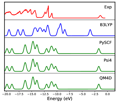
(a) GSC

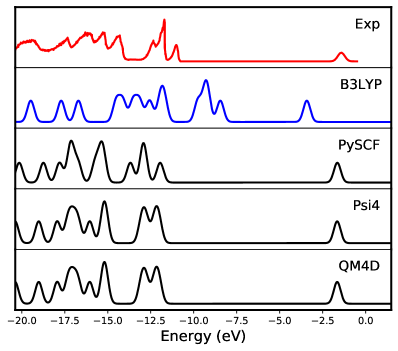
(b) post-LOSC2

Figure 2: Photoemission spectrum of maleic anhydride calculated from B3LYP, GSC, and post-LOSC2, compared with the experimental result⁶⁹.

To test the implementation of psi4_losc and pyscf_losc, IP values of polyacetylene (PA) molecules with 1 to 10 units were calculated with both Psi4 and PySCF and compared with the results from QM4D as shown in Table 2. These three software packages give mostly the same results for parent DFA calculations. The mean absolute errors (MAEs) differ by 0.01 eV for post-LOSC2 results and 0.02 eV for SCF-LOSC2 results. This shows that the integration of LibSC with both Psi4 and PySCF is correct.

MAEs for the same test sets calculated with Psi4 and QM4D are listed in Table 3. The difference between the numbers is due to the fact that the MAE values are not calculated with exactly the same systems for each set. We could only get the results for a subset of the systems because of the SCF convergence issue of DFT. Detailed results are documented in the Supporting Information.

The photoemission spectrum of maleic anhydride is calculated from B3LYP, GSC, and post-LOSC2 with all the three software packages. The results are plotted and compared with both experimental⁶⁹ and B3LYP spectra in Figure 2. For the B3LYP spectrum, only QM4D result is shown because the three software packages produce the same result. These spectra show that both GSC and post-LOSC2 greatly correct the behavior of the parent DFA. On the experimental curve, the peak with the highest energy represents the LUMO energy, which is about $-$1.3 eV. The second peak from the right represents the HOMO energy, which should be about $-$11 eV. The HOMO-LUMO gap is about 10 eV. However, B3LYP gives a HOMO of about $-$8.5 eV and a LUMO of about $-$3.5 eV, and the HOMO-LUMO gap is about 5 eV, which is about 5 eV smaller than the experimental one. Both GSC and post-LOSC2 give nearly the same LUMO energy as the experimental one. The GSC HOMO is about 1 eV higher than the experimental HOMO energy, which gives a HOMO-LUMO gap about 1 eV smaller than the experimental gap. The post-LOSC2 HOMO energy is about 1 eV lower than the experimental value, and the HOMO-LUMO gap is about 1 eV wider than the experimental gap. Compared with the B3LYP spectrum, GSC and post-LOSC2 spectra can describe the energy structure of this system better.

4.3 Multi-minimum Problem with the Localization Procedure

The spectra shown in Figure 2 also indicate that the minimization of the cost function can have different local solutions. For GSC calculations, the localization process in Figure 1 is skipped, and the SC correction only comes from the curvature. As shown in Figure 2(a), without the localization process, the GSC spectra have no noticeable difference. On the other hand, for the post-LOSC2 calculations, the SC correction comes from both localization contribution and curvature contribution. With the contribution from the localization process included, as shown in Figure 2(b), difference between post-LOSC2 spectra shows up. There is one peak at around 13 eV in the PySCF spectrum which does not exist in other two spectra, and the peak at around 15.7 eV which appears in the Psi4 curve and the QM4D curve is missing from the PySCF curve. These differences, especially the differences between the PySCF spectrum and the Psi4 spectrum, which were calculated using the same C++ core code, indicate that the localization process happened differently for this system.

The problem is not with the implementation of LibSC. Repeating the same calculation with QM4D but starting the localization process from different initial guesses can also result in different solutions. Table 4 shows the results of 9 tests, for which the localization procedure started with 9 random $U$ matrices. Seven of the nine tests gave similar HOMO energies which are around $-$7.19 eV, while the other two HOMO energies are about $-$6.67 eV. The HOMO energy difference between these two groups is about 0.5 eV, which is close to the MAE of post-LOSC2 for the IP test set as shown in Table 3. In principle, the global minimum of the localization cost function, Eq. 6 , should be the unique answer. However, as shown in the fifth column of the table, the cost function can have different values. For a given system, $\langle r^{2}\rangle$ is a constant, and can be subtracted from the the cost function. Column 6 lists the relative cost function values of each test with respect to that of the first test. Tests 7 and 8 have the closest values of the cost function, but the HOMO energies differ by about 0.5 eV. On the other hand, the multi-minimum issue does not have significant influence on the total energy. When the HOMO energy is about $-$6.67 eV, the total energy is a little lower, but the maximum difference is less than 0.0001 Hartree. Although tests 8 and 9 give lower total energies, it is not evident that they offer better solutions. The cost function but not the total energy is the target function of the localization procedure. Unfortunately, the values of the cost function differ by about 0.5 a.u.² for tests 8 and 9, which means that they give very different local solutions.

Table 4: HOMO energies (in eV), LUMO energies (in eV), HOMO-LUMO gap (in eV), cost function ($F^{\sigma}-\langle r^{2}\rangle$) values (in a.u.²), relative cost function values (in a.u.), and total energies (in a.u.²) from post-LOSC2 calculations with default $\gamma$ (0.707) for the 4-unit polyacene molecule starting from random initial guesses. The calculations were done with QM4D. The localization procedure was done with the energy window of [$-$30, 10].

test	$\varepsilon_{\text{HOMO}}$	$\varepsilon_{\text{LUMO}}$	gap	$F^{\alpha}-\langle r^{2}\rangle$	$\Delta F^{\alpha}$	$E_{\text{total}}$
1	$-$7.18545464	$-$0.76867342	6.41678122	1106.627980	0	$-$693.4080891
2	$-$7.18574992	$-$0.77368498	6.41206494	1105.017501	$-$1.610479	$-$693.4080853
3	$-$7.18638324	$-$0.77317354	6.41320970	1106.165982	$-$0.461998	$-$693.4080848
4	$-$7.18543475	$-$0.76846903	6.41696572	1106.060276	$-$0.567704	$-$693.4080890
5	$-$7.18543353	$-$0.76846797	6.41696556	1104.974744	$-$1.653236	$-$693.4080884
6	$-$7.18575067	$-$0.77368597	6.41206470	1104.560970	$-$2.067010	$-$693.4080853
7	$-$7.18543678	$-$0.76847004	6.41696674	1104.501397	$-$2.126583	$-$693.4080884
8	$-$6.67494957	$-$0.77259372	5.90235585	1104.459009	$-$2.168971	$-$693.4081312
9	$-$6.67494986	$-$0.77259475	5.90235511	1106.001484	$-$0.626496	$-$693.4081104

To further investigate the multi-minimum problem, additional post-LOSC2 calculations were performed, with the energy component of the cost function ignored by setting the value of $\gamma$ in Eq. 6 to 0. The results are shown in Table 5. With only the spacial component included in the cost function, the absolute $\Delta F^{\alpha}$ values are smaller than those in Table 4. This suggests that including the energy component in the cost function can cause the surface of the cost function to be more rugged. The total energies agree to 0.001 a.u.. This is another evidence that the localization procedure does not affect the total energy by much.

Table 5: HOMO energies (in eV), LUMO energies (in eV), HOMO-LUMO gap (in eV), cost function ($F^{\sigma}-\langle r^{2}\rangle$) values (in a.u.²), relative cost function values (in a.u.²), and total energies (in a.u.) from post-LOSC2 calculations with $\gamma=0.00$ for the 4-unit polyacene molecule starting from random initial guesses. The calculations were done with QM4D. Energy window: [$-$30, 10].

test	$\varepsilon_{\text{HOMO}}$	$\varepsilon_{\text{LUMO}}$	gap	$F^{\alpha}-\langle r^{2}\rangle$	$\Delta F^{\alpha}$	$E_{\text{total}}$
1	$-$8.14696460	0.72329534	8.87025994	1570.28672	0	$-$693.3591227
2	$-$8.14507486	0.71698648	8.86206134	1570.75105	0.46433	$-$693.3583495
3	$-$8.14299246	0.71400910	8.85700156	1570.53514	0.24843	$-$693.3591227
4	$-$8.16482969	0.73987472	8.90470441	1570.33667	0.04995	$-$693.3595938
5	$-$8.16672873	0.74241664	8.90914537	1570.54338	0.25666	$-$693.3590521
6	$-$8.17631887	0.75790963	8.93422850	1569.94037	$-$0.34635	$-$693.3573091
7	$-$8.14824556	0.72607677	8.87432233	1570.34364	0.05693	$-$693.3575385
8	$-$8.14695585	0.72331595	8.87027180	1570.28789	0.00117	$-$693.3576098
9	$-$8.14590040	0.71864483	8.86454523	1570.72905	0.44234	$-$693.3585760

Data in Tables 4 and 5 show that the energy component can cause the cost function surface to be more rugged. To study the effect of including virtual orbitals, a new set of tests were done with only all the occupied orbitals included in the localization procedure. The results are shown in Table 6. With $\gamma$ set to zero and no virtual orbital included, the localization procedure becomes the original Foster-Boys localization⁷⁰. The value of the cost function is very stable. There is no noticeable difference between the cost function values of these tests, and the HOMO energies agree to the fifth digits after the decimal point. Thus, only one solution was found for the Foster-Boys localization. Compared with Table. 5, this suggests that including virtual orbitals in the localization procedure causes the smooth surface of the original Foster-Boys target function to become more rugged.

We conclude that the localization procedure is very sensitive to the starting point. Both including the virtual orbitals in the localization process and adding the energy component in the cost function contribute to the roughness of the cost function landscape. While multiple patterns of localization were observed, the total energy is not significantly affected, and the HOMO energy difference is about the same magnitude of the MAE of post-LOSC2 for the IP test set. Differences between post-LOSC2 spectra shown in Figure 2 can be attributed to the slight differences between the converged DFT results from the three software packages. Currently, it remains a challenge to overcome this multi-minimum problem.

Fortunately, the multi-minimum problem may not be a serious issue in practical calculations. Using a random $U$ matrix as the starting point of the localization is just for a testing purpose. In practical calculations, the initial $U$ matrix is usually an identity matrix, meaning the use of CO as the initial guess. Ten tests, for which the localization procedure started from an identity $U$ matrix, were performed on each of three different computers. Detailed data from these tests are documented in the Supporting Information. The behavior of the localization procedure is very stable. Results calculated by the same computers including frontier orbital energies, cost function values, and total energies are completely identical. The difference between data calculated by different computers is negligible. The difference between HOMO energies is about $2\times 10^{-5}$ eV. Although currently there is no effective way to make sure that the global minimum of the cost function is obtained, the same local minimum can be obtained by keep using the identity matrix as the initial $U$ matrix. This can also be verified by the fact that the Psi4 results agree with the QM4D results.

Table 6: HOMO energies (in eV), cost function ($F^{\alpha}-\langle r^{2}\rangle$) values (in a.u.²), relative cost function values (in a.u.²), and total energies (in a.u.) from post-LOSC2 calculations with $\gamma=0.00$ for the 4-unit polyacene molecule starting from random initial guesses of the $U$ matrix. The calculations were done with QM4D. Only occupied orbitals were included in the localization procedure.

test	$\varepsilon_{\text{HOMO}}$	$F^{\alpha}-\langle r^{2}\rangle$	$\Delta F^{\alpha}$	$E_{\text{total}}$
1	$-$9.08660137	289.22246	0	$-$693.4083449
2	$-$9.08660080	289.22246	0	$-$693.4083449
3	$-$9.08660401	289.22246	0	$-$693.4083449
4	$-$9.08660259	289.22246	0	$-$693.4083449
5	$-$9.08660203	289.22246	0	$-$693.4083449
6	$-$9.08660303	289.22246	0	$-$693.4083449
7	$-$9.08660383	289.22246	0	$-$693.4083449
8	$-$9.08660194	289.22246	0	$-$693.4083449
9	$-$9.08660198	289.22246	0	$-$693.4083449

5 Conclusion

In summary, we developed a reliable, flexible and open-source library LibSC for the scaling correction methods, which supports the GSC and LOSC methods at the present stage. The consistent and simple interfaces to multiple programming languages, including C, C++ and Python, are carefully designed to be user-friendly. We also applied LibSC in two open-source quantum chemistry packages, Psi4 and PySCF. With the distribution of LibSC and its implementation, the scaling correction methods should be available for broader applications. Y. M, J.Y. and Z.C. acknowledge the support from the National Institute of General Medical Sciences of the National Institutes of Health under award number R01-GM061870. W.Y. acknowledges the support from the National Science Foundation (grant no. CHE-1900338). Y. M. was also supported by the Shaffer-Hunnicutt Fellowship and Z.C. by the Kathleen Zielik Fellowship from Duke University. N.Q.S. acknowledges the support from the National Natural Science Foundation of China (grant no. 22073049), Supporting Information Available: computational details and numerical results.

Figure 3: For Table of Contents Only

References

- Hohenberg and Kohn 1964 Hohenberg, P.; Kohn, W. Inhomogeneous Electron Gas. Phys. Rev. 1964, 136, B864–B871
- Kohn and Sham 1965 Kohn, W.; Sham, L. J. Self-Consistent Equations Including Exchange and Correlation Effects. Phys. Rev. 1965, 140, A1133–A1138
- Parr and Yang 1989 Parr, R. G.; Yang, W. Density-Functional Theory of Atoms and Molecules; International Series of Monographs on Chemistry; Oxford University Press: Oxford, New York, 1989
- Vosko et al. 1980 Vosko, S. H.; Wilk, L.; Nusair, M. Accurate Spin-Dependent Electron Liquid Correlation Energies for Local Spin Density Calculations: A Critical Analysis. Can. J. Phys. 1980, 58, 1200–1211
- Perdew and Wang 1992 Perdew, J. P.; Wang, Y. Accurate and Simple Analytic Representation of the Electron-Gas Correlation Energy. Phys. Rev. B 1992, 45, 13244–13249
- Becke 1988 Becke, A. D. Density-Functional Exchange-Energy Approximation with Correct Asymptotic Behavior. Phys. Rev. A 1988, 38, 3098–3100
- Lee et al. 1988 Lee, C.; Yang, W.; Parr, R. G. Development of the Colle-Salvetti Correlation-Energy Formula into a Functional of the Electron Density. Phys. Rev. B 1988, 37, 785–789
- Perdew et al. 1996 Perdew, J. P.; Burke, K.; Ernzerhof, M. Generalized Gradient Approximation Made Simple. Phys. Rev. Lett. 1996, 77, 3865–3868
- Becke 1993 Becke, A. D. A new mixing of Hartree–Fock and local density-functional theories. The Journal of chemical physics 1993, 98, 1372–1377
- Stephens et al. 1994 Stephens, P. J.; Devlin, F. J.; Chabalowski, C. F.; Frisch, M. J. Ab Initio Calculation of Vibrational Absorption and Circular Dichroism Spectra Using Density Functional Force Fields. J. Phys. Chem. 1994, 98, 11623–11627
- Adamo and Barone 1999 Adamo, C.; Barone, V. Toward Reliable Density Functional Methods without Adjustable Parameters: The PBE0 Model. J. Chem. Phys. 1999, 110, 6158–6170
- Ernzerhof and Scuseria 1999 Ernzerhof, M.; Scuseria, G. E. Assessment of the Perdew–Burke–Ernzerhof Exchange-Correlation Functional. J. Chem. Phys. 1999, 110, 5029–5036
- Mori-Sánchez et al. 2008 Mori-Sánchez, P.; Cohen, A. J.; Yang, W. Localization and Delocalization Errors in Density Functional Theory and Implications for Band-Gap Prediction. Phys. Rev. Lett. 2008, 100, 146401
- Cohen et al. 2008 Cohen, A. J.; Mori-Sánchez, P.; Yang, W. Fractional Charge Perspective on the Band Gap in Density-Functional Theory. Phys. Rev. B 2008, 77, 115123
- Cohen et al. 2008 Cohen, A. J.; Mori-Sánchez, P.; Yang, W. Insights into Current Limitations of Density Functional Theory. Science 2008, 321, 792–794
- Cohen et al. 2012 Cohen, A. J.; Mori-Sánchez, P.; Yang, W. Challenges for Density Functional Theory. Chem. Rev. 2012, 112, 289–320
- Zhang and Yang 1998 Zhang, Y.; Yang, W. A Challenge for Density Functionals: Self-Interaction Error Increases for Systems with a Noninteger Number of Electrons. J. Chem. Phys. 1998, 109, 2604–2608
- Dutoi and Head-Gordon 2006 Dutoi, A. D.; Head-Gordon, M. Self-Interaction Error of Local Density Functionals for Alkali–Halide Dissociation. Chem. Phys. Lett. 2006, 422, 230–233
- Mori-Sánchez et al. 2006 Mori-Sánchez, P.; Cohen, A. J.; Yang, W. Many-Electron Self-Interaction Error in Approximate Density Functionals. J. Chem. Phys. 2006, 125, 201102
- Ruzsinszky et al. 2006 Ruzsinszky, A.; Perdew, J. P.; Csonka, G. I.; Vydrov, O. A.; Scuseria, G. E. Spurious Fractional Charge on Dissociated Atoms: Pervasive and Resilient Self-Interaction Error of Common Density Functionals. J. Chem. Phys. 2006, 125, 194112
- Vydrov et al. 2007 Vydrov, O. A.; Scuseria, G. E.; Perdew, J. P. Tests of Functionals for Systems with Fractional Electron Number. J. Chem. Phys. 2007, 126, 154109
- Zheng et al. 2012 Zheng, X.; Liu, M.; Johnson, E. R.; Contreras-García, J.; Yang, W. Delocalization Error of Density-Functional Approximations: A Distinct Manifestation in Hydrogen Molecular Chains. J. Chem. Phys. 2012, 137, 214106
- Savin and Flad 1995 Savin, A.; Flad, H.-J. Density Functionals for the Yukawa Electron-Electron Interaction. Int. J. Quantum Chem. 1995, 56, 327–332
- Savin 1996 Savin, A. In Theoretical and Computational Chemistry; Seminario, J. M., Ed.; Recent Developments and Applications of Modern Density Functional Theory; Elsevier, 1996; Vol. 4; pp 327–357
- Iikura et al. 2001 Iikura, H.; Tsuneda, T.; Yanai, T.; Hirao, K. A Long-Range Correction Scheme for Generalized-Gradient-Approximation Exchange Functionals. J. Chem. Phys. 2001, 115, 3540–3544
- Yanai et al. 2004 Yanai, T.; Tew, D. P.; Handy, N. C. A New Hybrid Exchange–Correlation Functional Using the Coulomb-Attenuating Method (CAM-B3LYP). Chem. Phys. Lett. 2004, 393, 51–57
- Vydrov and Scuseria 2006 Vydrov, O. A.; Scuseria, G. E. Assessment of a Long-Range Corrected Hybrid Functional. J. Chem. Phys. 2006, 125, 234109
- Chai and Head-Gordon 2008 Chai, J.-D.; Head-Gordon, M. Long-Range Corrected Hybrid Density Functionals with Damped Atom–Atom Dispersion Corrections. Phys. Chem. Chem. Phys. 2008, 10, 6615–6620
- Baer et al. 2010 Baer, R.; Livshits, E.; Salzner, U. Tuned range-separated hybrids in density functional theory. Annual review of physical chemistry 2010, 61, 85–109
- Perdew and Zunger 1981 Perdew, J. P.; Zunger, A. Self-Interaction Correction to Density-Functional Approximations for Many-Electron Systems. Phys. Rev. B 1981, 23, 5048–5079
- Mori-Sánchez et al. 2006 Mori-Sánchez, P.; Cohen, A. J.; Yang, W. Self-Interaction-Free Exchange-Correlation Functional for Thermochemistry and Kinetics. J. Chem. Phys. 2006, 124, 091102
- Perdew et al. 2008 Perdew, J. P.; Staroverov, V. N.; Tao, J.; Scuseria, G. E. Density Functional with Full Exact Exchange, Balanced Nonlocality of Correlation, and Constraint Satisfaction. Phys. Rev. A 2008, 78, 052513
- Schmidt et al. 2014 Schmidt, T.; Kraisler, E.; Kronik, L.; Kümmel, S. One-Electron Self-Interaction and the Asymptotics of the Kohn–Sham Potential: An Impaired Relation. Phys. Chem. Chem. Phys. 2014, 16, 14357–14367
- Pederson et al. 2014 Pederson, M. R.; Ruzsinszky, A.; Perdew, J. P. Communication: Self-Interaction Correction with Unitary Invariance in Density Functional Theory. J. Chem. Phys. 2014, 140, 121103
- Schmidt and Kümmel 2016 Schmidt, T.; Kümmel, S. One- and Many-Electron Self-Interaction Error in Local and Global Hybrid Functionals. Phys. Rev. B 2016, 93, 165120
- Yang et al. 2017 Yang, Z.-h.; Pederson, M. R.; Perdew, J. P. Full Self-Consistency in the Fermi-Orbital Self-Interaction Correction. Phys. Rev. A 2017, 95, 052505
- Borghi et al. 2014 Borghi, G.; Ferretti, A.; Nguyen, N. L.; Dabo, I.; Marzari, N. Koopmans-Compliant Functionals and Their Performance against Reference Molecular Data. Phys. Rev. B 2014, 90, 075135
- Colonna et al. 2019 Colonna, N.; Nguyen, N. L.; Ferretti, A.; Marzari, N. Koopmans-Compliant Functionals and Potentials and Their Application to the GW100 Test Set. J. Chem. Theory Comput. 2019, 15, 1905–1914
- Anisimov and Kozhevnikov 2005 Anisimov, V. I.; Kozhevnikov, A. V. Transition State Method and Wannier Functions. Phys. Rev. B 2005, 72, 075125
- Ma and Wang 2016 Ma, J.; Wang, L.-W. Using Wannier functions to improve solid band gap predictions in density functional theory. Scientific reports 2016, 6, 1–8
- Zheng et al. 2011 Zheng, X.; Cohen, A. J.; Mori-Sánchez, P.; Hu, X.; Yang, W. Improving Band Gap Prediction in Density Functional Theory from Molecules to Solids. Phys. Rev. Lett. 2011, 107, 026403
- Li et al. 2015 Li, C.; Zheng, X.; Cohen, A. J.; Mori-Sánchez, P.; Yang, W. Local Scaling Correction for Reducing Delocalization Error in Density Functional Approximations. Phys. Rev. Lett. 2015, 114, 053001
- Li et al. 2018 Li, C.; Zheng, X.; Su, N. Q.; Yang, W. Localized Orbital Scaling Correction for Systematic Elimination of Delocalization Error in Density Functional Approximations. Natl. Sci. Rev. 2018, 5, 203–215
- Su et al. 2020 Su, N. Q.; Mahler, A.; Yang, W. Preserving Symmetry and Degeneracy in the Localized Orbital Scaling Correction Approach. J. Phys. Chem. Lett. 2020, 11, 1528–1535
- Mei et al. 2020 Mei, Y.; Chen, Z.; Yang, W. Self-Consistent Calculation of the Localized Orbital Scaling Correction for Correct Electron Densities and Energy-Level Alignments in Density Functional Theory. J. Phys. Chem. Lett. 2020, 11, 10269–10277
- Mei et al. 2021 Mei, Y.; Chen, Z.; Yang, W. Exact Second-Order Corrections and Accurate Quasiparticle Energy Calculations in Density Functional Theory. J. Phys. Chem. Lett. 2021, 7236–7244
- Mei et al. 2019 Mei, Y.; Li, C.; Su, N. Q.; Yang, W. Approximating Quasiparticle and Excitation Energies from Ground State Generalized Kohn–Sham Calculations. J. Phys. Chem. A 2019, 123, 666–673
- Mei and Yang 2019 Mei, Y.; Yang, W. Charge Transfer Excitation Energies from Ground State Density Functional Theory Calculations. J. Chem. Phys. 2019, 150, 144109
- Mei and Yang 2019 Mei, Y.; Yang, W. Excited-State Potential Energy Surfaces, Conical Intersections, and Analytical Gradients from Ground-State Density Functional Theory. J. Phys. Chem. Lett. 2019, 10, 2538–2545
- Yang et al. 2020 Yang, X.; Zheng, X.; Yang, W. Density Functional Prediction of Quasiparticle, Excitation, and Resonance Energies of Molecules With a Global Scaling Correction Approach. Front. Chem. 2020, 8
- Mei et al. 2021 Mei, Y.; Yang, N.; Yang, W. Describing Polymer Polarizability with Localized Orbital Scaling Correction in Density Functional Theory. J. Chem. Phys. 2021, 154, 054302
- qm 4 An in-house program for QM/MM simulations; available from https://qm4d.org/
- Smith et al. 2020 Smith, D. G. A.; Burns, L. A.; Simmonett, A. C.; Parrish, R. M.; Schieber, M. C.; Galvelis, R.; Kraus, P.; Kruse, H.; Di Remigio, R.; Alenaizan, A. et al. PSI4 1.4: Open-Source Software for High-Throughput Quantum Chemistry. J. Chem. Phys. 2020, 152, 184108
- Sun et al. 2018 Sun, Q.; Berkelbach, T. C.; Blunt, N. S.; Booth, G. H.; Guo, S.; Li, Z.; Liu, J.; McClain, J. D.; Sayfutyarova, E. R.; Sharma, S. et al. PySCF: The Python-Based Simulations of Chemistry Framework. Wiley Interdiscip. Rev. Comput. Mol. Sci. 2018, 8, e1340
- Perdew et al. 1982 Perdew, J. P.; Parr, R. G.; Levy, M.; Balduz, J. L. Density-Functional Theory for Fractional Particle Number: Derivative Discontinuities of the Energy. Phys. Rev. Lett. 1982, 49, 1691–1694
- Yang et al. 2000 Yang, W.; Zhang, Y.; Ayers, P. W. Degenerate Ground States and a Fractional Number of Electrons in Density and Reduced Density Matrix Functional Theory. Phys. Rev. Lett. 2000, 84, 5172–5175
- Zhang and Yang 2001 Zhang, Y.; Yang, W. In Theoretical Chemistry Accounts: New Century Issue; Cramer, C. J., Truhlar, D. G., Eds.; Springer: Berlin, Heidelberg, 2001; pp 346–348
- Edmiston and Ruedenberg 1963 Edmiston, C.; Ruedenberg, K. Localized Atomic and Molecular Orbitals. Rev. Mod. Phys. 1963, 35, 457–464
- Vahtras et al. 1993 Vahtras, O.; Almlöf, J.; Feyereisen, M. W. Integral Approximations for LCAO-SCF Calculations. Chemical Physics Letters 1993, 213, 514–518
- Früchtl et al. 1997 Früchtl, H. A.; Kendall, R. A.; Harrison, R. J.; Dyall, K. G. An Implementation of RI–SCF on Parallel Computers. Int. J. Quantum Chem. 1997, 64, 63–69
- 61 Guennebaud, G.; Jacob, B. Eigen v3. Available: http://eigen.tuxfamily.org, 2010
- van der Walt et al. 2011 van der Walt, S.; Colbert, S. C.; Varoquaux, G. The NumPy Array: A Structure for Efficient Numerical Computation. Computing in Science & Engineering 2011, 13, 22–30
- Harris et al. 2020 Harris, C. R.; Millman, K. J.; van der Walt, S. J.; Gommers, R.; Virtanen, P.; Cournapeau, D.; Wieser, E.; Taylor, J.; Berg, S.; Smith, N. J. et al. Array Programming with NumPy. Nature 2020, 585, 357–362
- 64 Jakob, W.; Rhinelander, J.; Moldovan, D. pybind11 - Seamless operability between C++11 and Python. Available: https://github.com/pybind/pybind11, 2016
- Sun 2015 Sun, Q. Libcint: An efficient general integral library for G aussian basis functions. Journal of computational chemistry 2015, 36, 1664–1671
- 66 Source code and documentions are available at Github: https://github.com/Yang-Laboratory/losc, 2021
- Mei et al. 2020 Mei, Y.; Chen, Z.; Yang, W. Self-Consistent Calculation of the Localized Orbital Scaling Correction for Correct Electron Densities and Energy-Level Alignments in Density Functional Theory. J. Phys. Chem. Lett. 2020, 11, 10269–10277
- Mei et al. 2019 Mei, Y.; Li, C.; Su, N. Q.; Yang, W. Approximating Quasiparticle and Excitation Energies from Ground State Generalized Kohn-Sham Calculations. 2019,
- Knight et al. 2016 Knight, J. W.; Wang, X.; Gallandi, L.; Dolgounitcheva, O.; Ren, X.; Ortiz, J. V.; Rinke, P.; Körzdörfer, T.; Marom, N. Accurate ionization potentials and electron affinities of acceptor molecules III: a benchmark of GW methods. Journal of chemical theory and computation 2016, 12, 615–626
- Boys 1960 Boys, S. F. Construction of some molecular orbitals to be approximately invariant for changes from one molecule to another. Reviews of Modern Physics 1960, 32, 296