Film Trailer Generation via Task Decomposition

Abstract

Movie trailers perform multiple functions: they introduce viewers to the story, convey the mood and artistic style of the film, and encourage audiences to see the movie. These diverse functions make automatic trailer generation a challenging endeavor. We decompose it into two subtasks: narrative structure identification and sentiment prediction. We model movies as graphs, where nodes are shots and edges denote semantic relations between them. We learn these relations using joint contrastive training which leverages privileged textual information (e.g., characters, actions, situations) from screenplays. An unsupervised algorithm then traverses the graph and generates trailers that human judges prefer to ones generated by competitive supervised approaches.

1 Introduction

Trailers are short videos used for promoting movies and are often critical to commercial success. While their core function is to market the film to a range of audiences, trailers are also a form of persuasive art and promotional narrative, designed to make viewers want to see the movie. Even though the making of trailers is considered an artistic endeavor, the film industry has developed strategies guiding trailer construction. According to one school of thought, trailers must exhibit a narrative structure, consisting of three acts. The first act establishes the characters and setup of the story, the second act introduces the main conflict, and the third act raises the stakes and provides teasers from the ending. Another school of thought is more concerned with the mood of the trailer as defined by the ups and downs of the story. According to this approach, trailers should have medium intensity at first in order to captivate viewers, followed by low intensity for delivering key information about the story, and then progressively increasing intensity until reaching a climax at the end of the trailer.

To create trailers automatically, we need to perform low-level tasks such as person identification, action recognition, and sentiment prediction, but also more high-level ones such as understanding connections between events and their causality, as well as drawing inferences about the characters and their actions. Given the complexity of the task, directly learning all this knowledge from movie-trailer pairs would require many thousands of examples, whose processing and annotation would be a challenge. It is thus not surprising that previous approaches to automatic trailer generation [24, 46, 53] have solely focused on audiovisual features.

Inspired by the creative process of human editors, we adopt a bottom-up approach to trailer generation, which we decompose into two orthogonal, simpler and well-defined subtasks. The first is the identification of narrative structure, i.e., retrieving the most important events of the movie. A commonly adopted theory in screenwriting [13, 22, 51] suggests that there are five types of key events in a movie’s plot, known as turning points (TPs; see their definitions in Figure 1). The second subtask is sentiment prediction, which we view as an approximation of flow of intensity between shots and the emotions evoked.

1. Opportunity	Introductory event that occurs after presentation of setting and background of main characters.
2. Change of Plans	Main goal of story is defined; action begins to increase.
3. Point of No Return	Event that pushes the characters to fully commit to their goal.
4. Major Setback	Event where everything falls apart, temporarily or permanently.
5. Climax	Final event of the main story, moment of resolution.

Figure 1: Turning points and their definitions.

We generate proposal trailers following an unsupervised graph-based approach. We model movies as graphs whose nodes are shots and whose edges denote important semantic connections between shots (see Figure 3). In addition, nodes bear labels denoting whether they are key events (i.e., TPs) and scores signaling sentiment intensity (positive or negative). Our algorithm traverses this movie graph to create trailer sequences. These could be used as proposals to be reviewed and modified by a human editor.

Both the tasks of TP identification and sentiment prediction stand to benefit from a lower-level understanding of movie content. Indeed, we could employ off-the-shelf modules for identifying characters and places, recognizing actions, and localizing semantic units. However, such approaches substantially increase pre-processing time and memory requirements during training and inference and suffer from error propagation. Instead, we propose a contrastive learning regime, where we take advantage of screenplays as privileged information, i.e., information available at training time only. Screenplays reveal how the movie is segmented into scenes, who the characters are, when and who they are speaking to, where they are and what they are doing (i.e., “scene headings” explain where the action takes place while “action lines” describe what the camera sees). Specifically, we build two individual networks, a textual network based on screenplays and a multimodal one based on video, and train them jointly using auxiliary contrastive losses. The textual network can additionally be pretrained on large collections of screenplays via self-supervised learning, without having to collect and process the corresponding movies. Experimental results show that this contrastive training approach is beneficial, leading to trailers which are judged favorably by humans in terms of their content and attractiveness.

2 Related Work

Previous approaches to movie understanding have mainly focused on isolated video clips, and tasks such as the alignment between movie scenes and book chapters [49], question answering [50], video captioning for movie shots [44], and text-to-video retrieval [5]. Recent work [41, 40, 42] attempts to identify high-level narrative structure and summarize entire TV episodes and movies focusing exclusively on the textual modality (i.e., screenplays).

Existing approaches to trailer generation exploit superficial audiovisual features, such as background music or visual changes between sequential shots [24, 46]. Other work creates “attractive” trailers with a graph-based model for shot selection [57] or uses a human in the loop in conjunction with a model trained on horror movies via audiovisual sentiment analysis [47]. The Trailer Moment Detection Dataset [53] consists of full-length movies paired with official trailers and annotations for key moments, but it is not publicly available and does not include screenplays.

Knowledge distillation [3, 23] was originally proposed for distilling information from a larger teacher model to a smaller student one. Generalized distillation [30] provides a framework for using privileged information, i.e., information which is available at training time only. Most related to our work is the use of different modalities or views of the same content [34, 33], e.g., transcribed narrations to learn visual representations in instructional videos. We leverage screenplays as a source of privileged information and distill knowledge about events, characters, and scenes in a film, which we subsequently exploit for identifying trailer-worthy shots in video.

3 Problem Formulation

Trailer generation requires the selection of $L$ shots from a full-length movie of $M$ shots ($L\ll M$). Movies present complex stories that may contain distinct subplots or events that unfold non-linearly, while redundant events, called “fillers” enrich the main story. Hence, we cannot assume that consecutive shots are necessarily semantically related. To better explore relations between events, we represent movies as graphs [42]. Let $\mathcal{G}=(\mathcal{V},\mathcal{E})$ denote a graph where vertices $\mathcal{V}$ are shots and edges $\mathcal{E}$ represent their semantic similarity. We further consider the original temporal order of shots in $\mathcal{G}$ by only allowing directed edges from previous to future shots. $\mathcal{G}$ is described by an upper-triangular transition matrix $\mathcal{T}$, which records the probability of transitioning from shot $i$ to every future shot $j$.

Within $\mathcal{G}$, we assume that some shots describe key events in the movie (thick circles in Figure 3) while all shots have a sentiment (positive or negative), whose intensity is denoted by a score (shades of green/red in Figure 3). We propose an algorithm for traversing $\mathcal{G}$ and selecting sequences of trailer shots. In the following, we first describe this algorithm (Section 3.1) and then discuss how the graph $\mathcal{G}$ is learned and key events are detected via TP identification [41] (Section 3.2). Finally, we also explain how shot-based sentiment scores are predicted (Section 3.5).

3.1 Movie Graph Traversal

Algorithm 1 Graph traversal: Retrieve trailer path

Input: shot-level graph $\mathcal{G}$, sets of TP shots, sentiment scores for all shots
Output: proposal trailer path (Path)

1:procedure GraphTrailer

2:    Path $\leftarrow\emptyset$, budget $\leftarrow L$, TPs_id $\leftarrow 0$, flow $\leftarrow\emptyset$

3:    events $\leftarrow$ $[\mathcal{TP}_{1},\mathcal{TP}_{2},\mathcal{TP}_{3},\mathcal{TP}_{4},\mathcal{TP}_{5}]$

4:    i $\leftarrow$ sample($\mathcal{TP}_{1}$)

5:    add i to Path

6:    next_TP $\leftarrow$ events[TPs_id]

7:    while budget $>0$ $\And$ TPs_id $<5$ do

8:         next_node $\vcentcolon=\operatornamewithlimits{argmax}\limits_{j\in\mathbb{N}_{i}}(s_{ij})$ $\triangleright$ Eq. 2

9:         add next_node to Path

10:         add sentiment(next_node) to flow

11:         i $\leftarrow$ next_node

12:         budget++

13:         if i $\in$ next_TP $\cup$ $\mathcal{N}_{next\_TP}$ then

14:             TPs_id++,   next_TP $\leftarrow$ events[TPs_id]              return Path

Algorithm 1 retrieves trailer sequences by performing random walks in graph $\mathcal{G}$. We start by selecting a node identified as the first TP (i.e., Opportunity, see Figure 1). Note that TPs extend over $C$ shots and as a result, our algorithm can produce $C$ different paths as proposal trailers (see line 4 in Algorithm 1). Given node $i$, we decide where to go next by considering its $K$ immediate neighbors $\mathcal{N}_{i}$. We select node $j$ from $\mathcal{N}_{i}$ as the $k^{\mathit{th}}$ shot $n_{k}$ to add to the path based on the following criteria: (1) normalized probability of transition $e_{ij}$ from $i$ to $j$ based on matrix $\mathcal{T}$ (i.e., semantic similarity between shots), (2) normalized distance $t_{ij}$ between shots $i$ and $j$ in the movie (i.e., temporal proximity), (3) normalized shortest path from node $j$ to next major event $d_{i,\mathcal{TP}}$ (i.e., relevance to the storyline), and (4) sentiment difference $p_{ij}$ from $i$ to $j$ based on the desired sentiment flow $f_{k}$ at the $k^{\mathit{th}}$ step in the path (see Section 3 and Appendix):

$$n_{k}=\operatornamewithlimits{argmax}\limits_{j\in\mathcal{N}_{i}}s_{ij}$$ (1)

$$s_{ij}=\lambda_{1}e_{ij}-\lambda_{2}t_{ij}-\lambda_{3}d_{i,\mathcal{TP}}-\lambda_{4}|p_{ij}-f_{k}|$$ (2)

where $\lambda_{1},\lambda_{2},\lambda_{3},\lambda_{4}$ are hyperparameters used to combine the different criteria (tuned on the development set based on ground-truth trailers). Note that these criteria are interpretable and can be easily altered by a user (e.g., add/delete a criterion, define a different flow $f$). Our approach could therefore be used for interactive trailer generation (which we do not pursue here, but see Appendix for an illustration).

We select $L$ shots in total (depending on a target trailer length) and retrieve a proposal trailer sequence as depicted in Figure 3 (bold line). At each step, we keep track of the sentiment flow created and the TPs identified thus far (lines 10 and 13–14 in Algorithm 1, respectively). A TP event has been selected for presentation in the trailer if a shot or its immediate neighbors have been added to the path.

3.2 TP Identification

Video-based Network

Let $\mathcal{F}$ denote a movie consisting of $M$ shots $\mathcal{F}=\{h_{1},h_{2},\dots,h_{M}\}$. A neural network model computes the probability $p(y_{it}|h_{i},\mathcal{F},\theta_{1})$, where $y_{it}$ is a binary label denoting whether shot $h_{i}$ represents TP $t\in[1,T]$ and $\theta_{1}$ are network parameters. Following screenwriting conventions [22], we assume there are five TPs ($T=5$) in a movie (see Figure 1).

We learn to identify TPs and the graph $\mathcal{G}$ that serves as input to our trailer generation algorithm in tandem. We hypothesize that the training signal provided by TP labels (i.e., the narrative structure) also encourages exploring meaningful semantic connections between shots via the graph that is learnt [42]. Each shot $i$ is represented by $h_{i}$, a nonlinear combination of textual, visual, and acoustic modalities $h_{i}=f([t_{i}^{\prime};v_{i}^{\prime};a_{i}^{\prime}])$, where $f(\cdot)$ is a fully-connected layer followed by the ReLU non-linearity. We compute textual representation $t_{i}^{\prime}$ via the bi-directional attention flow [45, 27] between subtitles $t_{i}$ and two other modalities, namely audio $a_{i}$ and video frames $v_{i}$:

$$S_{t_{i},a_{i}}=a_{i}^{T}t_{i},\quad S_{t_{i},v_{i}}=v_{i}^{T}t_{i}$$ (3)

$$a_{i,att}=\operatorname{r}(S_{t_{i},a_{i}})a_{i},\quad v_{i,att}=\operatorname{r}(S_{t_{i},v_{i}})v_{i}$$ (4)

$$t_{i}^{\prime}=a_{i,att}+v_{i,att}+t_{i}$$ (5)

where $\operatorname{r}$ is the softmax function. The final audio $a_{i}^{\prime}$ and visual $v_{i}^{\prime}$ representations are obtained analogously. Before fusion, the modalities are projected to a lower dimension via a fully-connected linear layer and L2 normalization.

We initially construct a fully-connected graph by computing the pairwise similarity between all multimodal shot vectors $h_{1},h_{2},\dots,h_{M}$. In order to avoid dense connections in the graph, which lead to worse contextualization and computational overhead, we select a small but variable-length neighborhood per shot and we sparsify the graph accordingly. During sparsification, we also constrain the adjacency matrix of the graph to be upper triangular (i.e., allowing only future connections between shots). For more details about the graph sparsification, see [42] and the Appendix. We also contextualize all shots with respect to the whole movie using a transformer encoder [52] and additionally encode each shot via a one-layer Graph Convolution Network (GCN; [15, 26, 28]). Finally, we combine the global (transformer-based) and local (graph-based) representations for each shot in order to compute the probability $p(y_{it}|h_{i},\mathcal{F},\theta_{1})$. The network is trained by minimizing the binary cross-entropy loss. After training, we use the learned sparse graph $\mathcal{G}$ as input to Algorithm 1.

Figure 2: GraphTrailer: a movie is a graph whose nodes are shots and edges denote relations between them. Each shot is characterized by a sentiment score (green/red shades for positive/negative values) and labels describing important events (thick circles). Our algorithm performs walks in the graph (bold line) to generate proposal trailer sequences.

Figure 3: Two networks process different views of the movie with different degrees of granularity. The video-based network takes as input multimodal fine-grained shot representations based on the movie’s video stream. The screenplay-based network processes textual scene representations which are coarse-grained and based on the movie’s screenplay. The networks are trained jointly on TP identification with losses enforcing prediction and representation consistency between them.

Screenplay-based Network

We also use a screenplay-based network that has similar architecture to the video-based network described in the previous section, but it considers textual information only and produces scene-level TP predictions (see Figure 3). Let $\mathcal{D}=\{s_{1},s_{2},\dots,s_{N}\}$ denote a screenplay with a sequence of $N$ scenes. The screenplay-based network estimates scene-level probabilities $q(y_{it}|s_{i},\mathcal{D},\theta_{2})$, quantifying the extent to which scene $s_{i}$ corresponds to the $t^{\mathit{th}}$ TP. We represent scenes with a small transformer encoder which operates over sequences of sentence vectors. As with our video-based network, we compute contextualized scene representations; a transformer encoder over the entire screenplay yields global representations, while local ones are obtained with a one-layer GCN over a sparse scene-level graph.

The video-based model assumes access to shot-level TP labels. However, the only dataset for TP identification we are aware of is TRIPOD [41], which contains scene-level labels based on screenplays. To obtain more fine-grained labels, we project scene-based annotations to shots following a simple one-to-many mapping (see Section 4 for details). Since our training signal is unavoidably noisy, we hypothesize that access to screenplays would encourage the video-based model to select shots which are more representative for each TP. In other words, screenplays represent privileged knowledge and an implicit supervision signal, while alleviating the need for additional pre-processing during inference. Moreover, screenplays provide a wealth of additional information, e.g., about characters and their roles in a scene, or their actions and emotions (conveyed by lines describing what the camera sees). This information might otherwise be difficult to accurately localize in video. Also, unlabeled text corpora of screenplays are relatively easy to obtain and can be used to pre-train our network.

3.3 Knowledge Distillation

We now describe our joint training regime for the two networks which encapsulate different views of the movie in terms of data streams (multimodal vs. text-only) and their segmentation into semantic units (shots vs. scenes).

Prediction Consistency Loss

We aim to enforce some degree of agreement between the TP predictions of the two networks. For this reason, we train them jointly and introduce additional constraints in the loss objective. Similarly to knowledge distillation settings [3, 23], we utilize the KL divergence loss between the screenplay-based posterior distributions $q(y_{t}|\mathcal{D})$ and the video-based ones $p(y_{t}|\mathcal{F})$.

While in standard knowledge distillation settings both networks produce probabilities over the same units, in our case, one network predicts TPs for shots and the other one for scenes. We obtain scene-level probabilities $\overline{p(y_{t}|\mathcal{F})}$ by aggregating shot-level ones via max pooling and re-normalization. We then calculate the prediction consistency loss between the two networks as:

$$\mathcal{P}=\frac{1}{T}\sum_{t=1}^{T}\mathcal{D}_{KL}\left(\overline{p(y_{t}|\mathcal{F})}\,\,\middle\|\,q(y_{t}|\mathcal{D})\right)$$ (6)

Representation Consistency Loss

We propose using a second regularization loss between the two networks in order to also enforce consistency between the two graph-based representations (i.e., over video shots and screenplay scenes). The purpose of this loss is twofold: to improve TP predictions for the two networks, as shown in previous work on contrastive representation learning [38, 48, 39], and also to help learn more accurate connections between shots (recall that the shot-based graph serves as input to our trailer generation algorithm; Section 3.1). In comparison with screenplay scenes, which describe self-contained events in a movie, video shots are only a few seconds long and rely on surrounding context for their meaning. We hypothesize that by enforcing the graph neighborhood for a shot to preserve semantics similar to the corresponding screenplay scene, we will encourage the selection of appropriate neighbors in the shot-based graph.

We again first address the problem of varying granularity in the representations of the two networks. We compute an aggregated scene-level representation $\overline{h_{j}}$ based on shots $h_{i},\dots,h_{i+k}$ via mean pooling and calculate the noise contrastive estimation (NCE; [21, 55]) loss for the $j^{\mathit{th}}$ scene:

$$\mathcal{R}=-\frac{1}{N}\sum_{j=1}^{N}\log\frac{e^{s(\overline{h_{j}},s_{j})/\tau}}{e^{s(\overline{h_{j}},s_{j})/\tau}+\sum_{\begin{subarray}{c}k=1\\ k\neq j\end{subarray}}^{N}e^{s(\overline{h_{j}},s_{k})/\tau}}$$ (7)

where $s_{j}$ is the scene representation calculated by the GCN in the screenplay-based network, $\overline{h_{j}}$ is scene representation calculated by the GCN in the video-based network, $s(\cdot)$ is a similarity function (we use the scaled dot product between two vectors), and $\tau$ is a temperature hyperparameter.

Joint Training

Our final joint training objective takes into account the individual losses $\mathcal{S}$ and $\mathcal{V}$ of the screenplay- and video-based networks (see Appendix for details), and the two consistency losses $\mathcal{P}$ (for prediction) and $\mathcal{R}$ (for representation):

$$\mathcal{L}_{TP}=\mathcal{S}+\mathcal{V}+a\mathcal{P}+b\mathcal{R}$$ (8)

where $a,b$ are hyperparameters modulating the importance of prediction vs. representation consistency. Figure 3 provides a high-level illustration of our training regime.

3.4 Self-supervised Pretraining

Pretraining aims to learn better scene representations from screenplays which are more accessible than movie videos (e.g., fewer copyright issues and less computational overhead) in the hope that this knowledge will transfer to the video-based network via our consistency losses.

Pretraining takes place on Scriptbase [19], a dataset which consists of $\sim$1,100 full-length screenplays (approx. 140K scenes). We adapt, a self-supervised task, namely Contrastive Predictive Coding (CPC; [38]) to our setting: given a (contextualized) scene representation, we learn to predict a future representation in the movie. We consider a context window of several future scenes, rather than just one. This is an attempt to account for non-linearities in the movie, which can occur because of unrelated intervening events and subplots. Given the representation of an anchor scene $g_{i}$, a positive future representation $c_{i}^{+}$ and a set of negative examples $\{c_{i1}^{-},\dots,c_{i(N-1)}^{-}\}$, we compute the InfoNCE [38] loss:

$$\mathcal{L}_{\mathit{self}}=-\frac{1}{N}\sum_{j=1}^{N}\log\frac{e^{s(g_{i},c_{i}^{+})/\tau}}{e^{s(g_{i},c_{i}^{+})/\tau}+\sum_{k=1}^{N-1}e^{s(g_{i},c_{ik}^{-})/\tau}}$$ (9)

We obtain scene representations $g_{i}$ based on $s_{i}$ provided by the one-layer GCN. Starting from the current scene, we perform a random walk of $k$ steps and compute $g_{i}$ from the retrieved path $p_{i}$ in the graph via mean pooling (more details can be found in the Appendix).

3.5 Sentiment Prediction

Finally, our model takes into account how sentiment flows from one shot to the next. We predict sentiment scores per shot with the same joint architecture (Section 3.3) and training regime we use for TP identification. The video-based network is trained on shots with sentiment labels (i.e., positive, negative, neutral), while the screenplay-based network is trained on scenes with sentiment labels (Section 4 explains how the labels are obtained). After training, we predict a probability distribution over sentiment labels per shot to capture sentiment flow and discriminate between high- and low-intensity shots (see Appendix for details).

4 Experimental Setup

Datasets

Our model was trained on TRIPOD$\bigoplus$, an expanded version of the TRIPOD dataset [41, 42] which contains 122 screenplays with silver-standard TP annotations (scene-level) and the corresponding videos. For each movie, we further collected as many trailers as possible from YouTube, including official and (serious) fan-based ones, or modern trailers for older movies. To evaluate the trailers produced by our algorithm, we also collected a new held-out set of 41 movies. These movies were selected from the Moviescope dataset [11], which contains official movie trailers. The held-out set does not contain any additional information, such as screenplays or TP annotations. The statistics of TRIPOD$\bigoplus$ is presented in Table 1.

TRIPOD$\bigoplus$	Train	Dev+Test	Held-out
No. movies	84	38	41
No. scenes	11,320	5,830	—
No. video shots	81,400	34,100	48,600
No. trailers	277	155	41
Avg. movie duration	6.9k (0.6)	6.9k (1.3)	7.8k (2.3)
Avg. scenes per movie	133 (61)	153 (54)	—
Avg. shots per movie	968 (441)	898 (339)	1,186 (509)
duration	6.9 (15.1)	7.1 (13.6)	6.6 (16.6)
Avg. valid shots per movie	400 (131)	375 (109)	447 (111)
duration	13.5 (19.0)	13.9 (18.1)	13.3 (19.6)
Avg. trailers per movie	3.3 (1.0)	4.1 (1.0)	1.0 (0.0)
duration	137 (42)	168 (462)	148 (20)
Avg. shots per trailer	44 (27)	43 (27)	57 (28)
duration	3.1 (5.8)	3.9 (14.0)	2.6 (4.0)

Table 1: Statistics of TRIPOD$\bigoplus$ dataset (for movies, screenplays, trailers); standard deviation within brackets, duration in seconds.

Movie and Trailer Processing

The modeling approach put forward in previous sections assumes that we know the correspondence between screenplay scenes and movie shots. We obtain this mapping by automatically aligning the dialogue in screenplays with subtitles using Dynamic Time Warping (DTW; [36, 42]). We first segment the video into scenes based on this mapping, and then segment each scene into shots using PySceneDetect. Shots with less than 100 frames in total are too short for both processing and displaying as part of the trailer and are therefore discarded.

Moreover, for each shot we extract visual and audio features. We consider three different types of visual features: (1) We sample one key frame per shot and extract features using ResNeXt-101 [56] pre-trained for object recognition on ImageNet [14]. (2) We sample frames with a frequency of 1 out of every 10 frames (we increase this time interval for shots with larger duration since we face memory issues) and extract motion features using the two-stream I3D network pre-trained on Kinetics [10]. (3) We use Faster-RCNN [18] implemented in Detectron2 [54] to detect person instances in every key frame and keep the top four bounding boxes per shot which have the highest confidence alongside with the respective regional representations. We first project all individual representations to the same lower dimension and perform L2-normalization. Next, we consider the visual shot representation as the sum of the individual vectors. For the audio modality, we use YAMNet pre-trained on the AudioSet-YouTube corpus [16] for classifying audio segments into 521 audio classes (e.g., tools, music, explosion); for each audio segment contained in the scene, we extract features from the penultimate layer. Finally, we extract textual features [42] from subtitles and screenplay scenes using the Universal Sentence Encoder (USE; [12]).

For evaluation purposes, we need to know which shots in the movie are trailer-worthy or not. We do this by segmenting the corresponding trailer into shots and computing for each shot its visual similarity with all shots in the movie. Shots with highest similarity values receive positive labels (i.e., they should be in the trailer). However, since trailers also contain shots that are not in the movie (e.g., black screens with text, or simply material that did not make it in the final movie), we also set a threshold below which we do not map trailer shots to movie shots. In this way, we create silver-standard binary labels for movie shots.

Sentiment Labels

Since TRIPOD does not contain sentiment annotations, we instead obtain silver-standard labels via COSMIC [17], a commonsense-guided framework with state-of-the-art performance for sentiment and emotion classification in natural language conversations. Specifically, we train COSMIC on MELD [43], which contains dialogues from episodes of the TV series Friends and is more suited to our domain than other sentiment classification datasets (e.g., [9, 29]). After training, we use COSMIC to produce sentence-level sentiment predictions for the TRIPOD screenplays. The sentiment of a scene corresponds to the majority sentiment of its sentences. We project scene-based sentiment labels onto shots using the same one-to-many mapping employed for TPs.

5 Results and Analysis

Usefulness of Knowledge Distillation

We first investigate whether we improve TP identification, as it is critical to the trailer generation task. We split the set of movies with ground-truth scene-level TP labels into development and test set and select the top 5 (@5) and top 10 (@10) shots per TP in a movie. As evaluation metric, we consider Partial Agreement (PA; [41]), which measures the percentage of TPs for which a model correctly identifies at least one ground-truth shot from the 5 or 10 shots selected from the movie (see Appendix for details).

	PA@5$\uparrow$	PA@10$\uparrow$
Random (evenly distributed)	21.67	33.44
Theory position	10.00	12.22
Distribution position	12.22	15.56
GraphTP [42]	10.00	12.22
Transformer	22.22	33.33
GraphTrailer	27.78	35.56
+ Screenplay, Asynchronous ($\mathcal{P}$)	28.89	41.11
+ Screenplay, Asynchronous ($\mathcal{P}+\mathcal{R}$)	21.11	35.56
+ Screenplay, Contrastive Joint ($\mathcal{P}+\mathcal{R}$)	33.33	47.78
+ pre-training	34.44	50.00

Table 2: Model performance on TP identification (test set). GraphTrailer shown with different training regimes. Evaluation metric: Partial Agreement (PA) against top 5 (@5) and top 10 (@10) selected shots per TP and movie.

Table 2 summarizes our results on the test set. We consider the following comparison systems: Random selects shots from evenly distributed sections (average of 10 runs); Theory assigns TP to shots according to screenwriting theory (e.g., “Opportunity” occurs at 10% of the movie, “Change of plans” at 25%, etc.); Distribution selects shots based on their expected position in the training data; GraphTP is the original model of [42] trained on screenplays (we project scene-level TP predictions to shots); Transformer is a base model without graph-related information. We use our own model, GraphTrailer, in several variants for TP identification: without and with access to screenplays, trained only with the prediction consistency loss ($\mathcal{P}$), both prediction and representation losses ($\mathcal{P}+\mathcal{R}$), and our contrastive joint training regime.

We observe that GraphTrailer outperforms all baselines, as well the Transformer model. Although the latter encodes long-range dependencies between shots, GraphTrailer additionally benefits from directly encoding sparse connections learnt in the graph. Moreover, asynchronous knowledge distillation via the prediction consistency loss ($\mathcal{P}$) further improves performance, suggesting that knowledge contained in screenplays is complementary to what can be extracted from video. Notice that when we add the representation consistency loss ($\mathcal{P}+\mathcal{R}$), performance deteriorates by a large margin, whereas the proposed training approach (contrastive joint) performs best. Finally, pretraining offers further gains, albeit small, which underlines the benefits of the screenplay-based network.

	Dev$\uparrow$	Test$\uparrow$
Random selection w/o TPs	14.47	5.61
Random selection with TPs	20.00	9.27
TextRank [35]	10.26	3.66
GraphTrailer w/o TPs	23.58	11.53
GraphTrailer with TPs	26.95	16.44
CCANet [53]	31.05	15.12
Transformer	32.63	17.32
Supervised GraphTrailer	33.42	17.80
Upper bound	86.41	—

Table 3: Performance of unsupervised (upper part) and weakly supervised (lower part) models on trailer generation: accuracy of correctly identified trailer shots. All systems have the same shot budget for trailer creation.

Trailer Quality

We now evaluate the trailer generation algorithm of GraphTrailer on the held-out set of 41 movies (see Table 1). As evaluation metric, we use accuracy, i.e., the percentage of correctly identified trailer shots and we consider a total budget of 10 shots for the trailers in order to achieve the desired length ($\sim$2 minutes).

We compare GraphTrailer against several unsupervised approaches (first block in Table 3) including: Random selection among all shots and among TPs identified by GraphTrailer; we also implement two graph-based systems based on a fully-connected graph, where nodes are shots and edges denote the degree of similarity between them. This graph has no knowledge of TPs, it is constructed by calculating the similarity between generic multimodal representations. TextRank [35] operates over this graph to select shots based on their centrality, while GraphTrailer without TPs traverses the graph with TP and sentiment criteria removed (Equation 2). For the unsupervised systems which include stochasticity and produce proposals (Random, GraphTrailer), we consider the best proposal trailer. The second block of Table 3 presents supervised approaches which use noisy trailer labels for training. These include CCANet [53], which only considers visual information and computes the cross-attention between movie and trailer shots, and a vanilla Transformer trained for the binary task of identifying whether a shot should be in the trailer without considering screenplays, sentiment or TPs. Supervised GraphTrailer consists of our video-based network trained on the same data as the Transformer.

GraphTrailer performs best among unsupervised methods. Interestingly, TextRank is worse than random, illustrating that tasks like trailer generation cannot be viewed as standard summarization problems. GraphTrailer without TPs still performs better than TextRank and random TP selection. With regard to supervised approaches, we find that using all modalities with a standard architecture (Transformer) leads to better performance than sophisticated models using visual similarity (CCANet). By adding graph-related information (Supervised GraphTrailer), we obtain further improvements.

	Accuracy $\uparrow$
GraphTrailer	22.63
+ Auxiliary, Asynchronous ($\mathcal{P}$)	21.87
+ Auxiliary, Asynchronous ($\mathcal{P}+\mathcal{R}$)	22.11
+ Auxiliary, Contrast Joint ($\mathcal{P}+\mathcal{R}$)	25.44
+ pre-training	25.79

Table 4: Different training regimes for GraphTrailer: accuracy (%) of correctly identified trailer shots. For direct comparison GraphTrailer here only uses the narrative structure criterion, no information about sentiment intensity is considered.

	Accuracy $\uparrow$
Similarity	24.28
Similarity + TPs	25.79
Similarity + sentiment	23.97
Similarity + TPs + sentiment	26.95

Table 5: GraphTrailer with different criteria for performing random walks in the movie graph (Algorithm 1, Equation (2)).

We perform two ablation studies on the development set for GraphTrailer. The first study aims to assess how the different training regimes of the dual network influence downstream trailer generation performance. We observe in Table 4 that asynchronous training does not offer any discernible improvement over the base model. However, when we jointly train the two networks (video- and screenplay-based) using prediction and representation consistency losses, performance increases by nearly 3%. A further small increase is observed when the screenplay-based network is pre-trained on more data.

The second ablation study concerns the criteria used for performing random walks on the graph $\mathcal{G}$. As shown in Table 5, when we enforce the nodes in the selected path to be close to key events (similarity + TPs) performance improves. When we rely solely on sentiment (similarity + sentiment), performance drops slightly. This suggests that in contrast to previous approaches which mostly focus on superficial visual attractiveness [57, 53] or audiovisual sentiment analysis [47], sentiment information on its own is not sufficient and may promote outliers that do not fit well in a trailer. On the other hand, when sentiment information is combined with knowledge about narrative structure (similarity + TPs + sentiment), we observe the highest accuracy. This further validates our hypothesis that the two theories about creating trailers (i.e., based on narrative structure and emotions) are complementary and can be combined.

Finally, since we have multiple trailers per movie (for the dev set), we can measure the overlap between their shots (Upper bound). The average overlap is 86.14%, demonstrating good agreement between trailer makers and a big gap between human performance and automatic models.

	Q1	Q2	Best	Worst	BWS
Random selection w/o TPs	38.2	45.6	19.1	25.9	-1.26
GraphTrailer w/o TPs	37.2	44.5	24.4	25.9	-0.84
GraphTrailer w/ TPs	41.4	48.2	20.8	11.6	1.40
CCANet	37.7	46.6	14.3	15.2	-0.14
Superv. GraphTrailer	37.7	47.1	21.4	21.4	0.84

Table 6: Human evaluation on held-out set. Percentage of Yes answers for: Does the trailer contain sufficient information (Q1) and is it attractive (Q2). Percentage of times each system was selected as Best or Worst, and standardized best-worst scaling score.

Human Evaluation

We also conducted a human evaluation study to assess the quality of the generated trailers. For human evaluation, we include Random selection without TPs as a lower bound, the two best performing unsupervised models (i.e., GraphTrailer with and without TPs), and two supervised models: CCANet, which is the previous state of the art for trailer generation, and the supervised version of our model, which is the best performing model according to automatic metrics. We generated trailers for all movies in the held-out set. We then asked Amazon Mechanical Turk (AMT) crowd workers to watch all trailers for a movie, answer questions relating to the information provided (Q1) and the attractiveness (Q2) of the trailer, and select the best and worst trailer. We collected assessments from five different judges per movie.

Table 6 shows that GraphTrailer with TPs provides on average more informative (Q1) and attractive (Q2) trailers than all other systems. Although GraphTrailer without TPs and Supervised GraphTrailer are more often selected as best, they are also chosen equally often as worst. When we compute standardized scores (z-scores) using best-worst scaling [31], GraphTrailer with TPs achieves the best performance (note that is also rarely selected as worst) followed by Supervised GraphTrailer. Interestingly, GraphTrailer without TPs is most often selected as best (24.40%), which suggests that the overall approach of modeling movies as graphs and performing random walks instead of individually selecting shots helps create coherent trailers. However, the same model is also most often selected as worst, which shows that this naive approach on its own cannot guarantee good-quality trailers.

We include video examples of generated trailers based on our approach in the Supplementary Material. Moreover, we provide a step-by-step graphical example of our graph traversal algorithm in the Appendix.

Spoiler Alert!

Our model does not explicitly avoid spoilers in the generated trailers. We experimented with a spoiler-related criterion when traversing the movie graph in Algorithm 1. Specifically, we added a penalty when selecting shots that are in “spoiler-sensitive” graph neighborhoods. We identified such neighborhoods by measuring the shortest path from the last two TPs, which are by definition the biggest spoilers in a movie. However, this variant of our algorithm resulted in inferior performance and we thus did not pursue it further. We believe that such a criterion is not beneficial for proposing trailer sequences, since it discourages the model from selecting exciting shots from the latest parts of the movie. These high-tension shots are important for creating interesting trailers and are indeed included in real-life trailers. More than a third of professional trailers in our dataset contain shots from the last two TPs (“Major setback”, “Climax”). We discuss this further in the Appendix.

We also manually inspected the generated trailers and found that spoilers are not very common (i.e., we identified one major spoiler shot in a random sample of 12 trailers from the test set), possibly because the probability of selecting a major spoiler is generally low. And even if a spoiler-sensitive shot is included, when taken out of context it might not be enough to unveil the ending of a movie. However, we leave it to future work to investigate more elaborate spoiler identification techniques, which can easily be integrated to our algorithm as extra criteria.

6 Conclusions

In this work, we proposed a trailer generation approach which adopts a graph-based representation of movies and uses interpretable criteria for selecting shots. We also show how privileged information from screenplays can be leveraged via contrastive learning, resulting in a model that can be used for turning point identification and trailer generation. Trailers generated by our model were judged favorably in terms of their content and attractiveness.

In the future we would like to focus on methods for predicting fine-grained emotions (e.g., grief, loathing, terror, joy) in movies. In this work, we consider positive/negative sentiment as a stand-in for emotions, due to the absence of in-domain labeled datasets. Previous efforts have focused on tweets [1], Youtube opinion videos [4], talkshows [20], and recordings of human interactions [8]. Preliminary experiments revealed that transferring fine-grained emotion knowledge from other domains to ours leads to unreliable predictions compared to sentiment which is more stable and improves trailer generation performance. Avenues for future work include new emotion datasets for movies, as well as emotion detection models based on textual and audiovisual cues.

Appendix A Model Details

In this section we provide details about the various modeling components of our approach. We begin by providing details of the GraphTrailer architecture (Section A.1), then move to discuss how the TP identification network is trained (Section A.2), and finally give technical details about pre-training on screenplays (A.3), and the sentiment flow used for graph traversal (A.4).

A.1 GraphTrailer

As mentioned in the main paper, we assume a multimodal representation $h_{i}$ per shot based on movie subtitles, audio, and video frames. We then construct matrix $E$ by computing the pairwise similarity between all pairs of shots $h_{i},h_{j}$ in a movie:

$$e_{ij}=\tanh(W_{i}h_{i}+b_{i})\tanh(W_{j}h_{j}+b_{j})+b_{ij}$$ (10)

Similarities are normalized using the softmax function (row-wise normalization in matrix $E$). We thus obtain a fully-connected directed graph where edge $e^{\prime}_{ij}$ records the probability that $h_{i}$ is connected with $h_{j}$ in the graph. Next, we remove all edges from the graph which represent connections from future to past shots (i.e., we render adjacency matrix $E^{\prime}$ upper triangular by masking the positions below the diagonal). Finally, we sparsify the graph by selecting a top-$k$ neighborhood $\mathcal{P}_{i}$ per shot $h_{i}$: $\mathcal{P}_{i}=\operatorname{argmax}\limits_{j\in[1,M],|\mathcal{P}_{i}|=k}e^{\prime}_{ij}$. Instead of deciding on a fixed number of $k$ neighbors for all shots and movies, we determine a predefined set of options for $k$ (e.g., integer numbers contained in a set $O$) and learn to select the appropriate $k$ per shot via a parametrized function: $z_{i}=W_{n}e^{\prime}_{i}+b_{n}$, where $z_{i}$ is a probability distribution over the neighborhood size options for shot $h_{i}$. Hence, the final neighborhood size for shot $h_{i}$ is: $k_{i}=\operatorname{argmax}_{t\in O}z_{it}$.

We address discontinuities in our model (i.e., top-$k$ sampling, neighborhood size selection) by utilising the Straight-Through Estimator [7]. During the backward pass we compute the gradients with the Gumbel-softmax reparametrization trick [32, 25]. The same procedure is followed for constructing and sparsifying scene-level graphs in the auxiliary screenplay-based network.

A.2 Training on TP Identification

Section 3 presents our training regime for the video- and screenplay-based model assuming TP labels for scenes are available (i.e., binary labels indicating whether a scene acts as a TP in a movie). Given such labels, our model is trained with a binary cross-entropy loss (BCE) objective between the few-hot gold labels and the network’s TP predictions.

However, in practice, our training set contains silver-standard labels for scenes. The latter are released together with the TRIPOD [41] dataset and were created automatically. Specifically, TRIPOD provides gold-standard TP annotations for synopses (not screenplays), under the assumption that synopsis sentences are representative of TPs. And sentence-level annotations are projected to scenes with a matching model trained with teacher forcing [41] to create silver-standard labels.

In this work, we consider the probability distribution over screenplay scenes as produced by the teacher model for each TP and compute the KL divergence loss between the teacher posterior distributions $q(y_{t})$ and the ones computed by our model $p(y_{t})$:

$$\mathcal{O}_{t}=\mathcal{D}_{KL}\left(p(y_{t})\middle\|q(y_{t})\right),t\in[1,T]$$ (11)

where $T$ is the number of TPs. Hence, the loss $\mathcal{S}$ (Equation (8), Section 3.3) used for the auxiliary screenplay network is: $\mathcal{S}=\sum_{t=1}^{T}\mathcal{O}_{t}$ . Accordingly, for the video-based network which operates over shots, we first aggregate shot probabilities to scene-level ones (see Sections 3.3 and 4) and then compute the KL divergence between the aggregated probabilities and the teacher distribution (loss $\mathcal{V}$ in Equation (8), Section 3.3), in the same fashion as in Equation (11).

A.3 Self-supervised Pre-training

In Section 3.4, we describe a modified approach to Contrastive Predictive Coding (CPC; [38]) for pre-training the screenplay-based network on a larger corpus of screenplays (i.e., Scriptbase [19]). The training objective is InfoNCE (see Equation (9)) and considers structure-aware representations for each scene $s_{i}$ in the screenplay.

Here, we explain in more detail how these representations are computed. Given scene $s_{i}$, we select the next node in the path based on the edge weights connecting it to its neighbors $s_{t}=\operatorname{argmax}\limits_{j\in\mathcal{P}_{i}}e^{\prime}_{ij}$ where $\mathcal{P}_{i}$ is the sparsified immediate neighborhood for $s_{i}$. We perform $k$ such steps and create path $p_{i}$ which contains (graph-based) representations (via one-layer GCN) for the selected nodes. Finally, representation $g_{i}$ for scene $s_{i}$ is computed from this path $p_{i}$ via mean-pooling.

Notice that we compute structure-aware scene representations $g_{i}$ via random walks rather than stacking multiple GCN layers. We could in theory stack two or three GCN layers and thus consider many more representations (e.g., 100 or 1,000) for contextualizing $g_{i}$. However, this would result to over-smoothed representations, that converge to the same vector [37]. Moreover, when trying to contextualize such large neighborhoods in a graph, the bottleneck phenomenon prevents the effective propagation of long-range information [2] which is our main goal. Finally, in ”small world” networks with a few hops, neighborhoods could end up containing the majority of the nodes in the graph [6], which again hinders meaningful exploration of long-range dependencies. Based on these limitations of GCNs, we perform random walks, which allow us to consider a small number of representations when contextualizing a scene, while also exploring long-range dependencies.

A.4 Sentiment Flow in GraphTrailer

One of the criteria for selecting the next shot in our graph traversal algorithm (Section 3.1) is the sentiment flow of the trailer generated so far. Specifically, we adopt the hypothesis that trailers are segmented into three sections based on sentiment intensity. The first section has medium intensity for attracting viewers, the second section has low intensity for delivering key information about the movie and finally the third section displays progressively higher intensity for creating cliffhangers and excitement for the movie.

Accordingly, given a budget of $L$ trailer shots, we expect the first $L/3$ ones to have medium intensity without large variations within the section (e.g., we want shots with average absolute intensity close to 0.7, where all scores are normalized to a range from -1 to 1). In the second part of the trailer (i.e., the next $L/3$ shots) we expect a sharp drop in intensity and shots within this section to maintain more or less neutral sentiment (i.e., 0 intensity). Finally, for the third section (i.e., the final $L/3$ shots) we expect intensity to steadily increase. In practice, we expect the intensity of the first shot to be 0.7 (i.e., medium intensity), increasing by 0.1 with each subsequent shot until we reach a peak at the final shot.

Appendix B Implementation Details

Evaluation Metrics

Previous work [41] evaluates the performance of TP identification models in terms of three metrics: Total Agreement (TA), i.e., the percentage of TP scenes that are correctly identified, Partial Agreement (PA), i.e., the percentage of TP events for which at least one gold-standard scene is identified, and Distance (D), i.e., the minimum distance in number of scenes between the predicted and gold-standard set of scenes for a given TP, normalized by the screenplay length. We report results with the partial agreement metric. We can no longer use total agreement, since we evaluate against silver standard (rather than gold) labels for shots (rather than scenes) and as a result consider all shots within a scene equally important. We do not use the distance metric either since it yields very similar outcomes and does not help discriminate among model variants.

Hyperparameters

Following previous work [42], we project all types of features (i.e., textual, visual, and audio) to the same lower dimension of 128. We find that larger dimensions increase the number of parameters considerably and yield inferior results possibly due to small dataset size.

We contextualize scenes (with respect to the screenplay) and shots (with respect to the video) using transformer encoders. We experimented with 2, 3, 4, 5, and 6 layers in the encoder and obtained best results with 3 layers. For the feed forward (FF) dimension, we experimented with both a standard size of 2,048 and a smaller size of 1,024 and found the former works better. We use another transformer encoder to compute the representation of a scene from a sequence of input sentence representations. This encoder has 4 layers and 1,024 FF dimension. Both encoders, employ 8 attention heads and 0.3 dropout.

During graph sparsification (i.e., selection of top-$k$ neighbors), we consider different neighborhood options for the scene- and shot-based networks due to their different granularity and size. Following [42], we consider [1–6] neighbors for the scene network and we increase the neighborhood size to [6–12] for the shot network.

For training our dual network on TP identification, we use the $\mathcal{L}_{TP}$ objective described in Equation (8) (Section 3.3). We set hyperparameters $a$ and $b$ that determine the importance of the prediction and representation consistency losses in $\mathcal{L}_{TP}$ to 10 and 0.03, respectively. Moreover, while pre-training the screenplay-based network on the Scriptbase corpus [19] we select as future context window 10% of the screenplay. As explained in Sections 3.4 and A.3, we compute structure-aware scene representations by performing random walks of $k$ steps in the graph starting from an anchor scene. We empirically choose 3 steps.

Finally, as described in Section 3.1, GraphTrailer uses a combination of multiple criteria for selecting the next node to be included in the trailer path. The criteria are combined using hyperparameters which are tuned on the development set. The search space for each hyperparameter $\lambda$ (Equation (2), Section 3.1) is [0, 1, 5, 10, 15, 20, 25, 30] and we find that the best combination for $\lambda_{1}$ (semantic similarity), $\lambda_{2}$ (time proximity), $\lambda_{3}$ (narrative structure), and $\lambda_{4}$ (sentiment intensity) is [1, 5, 10, 10], respectively.

Appendix C Results: Ablation Studies

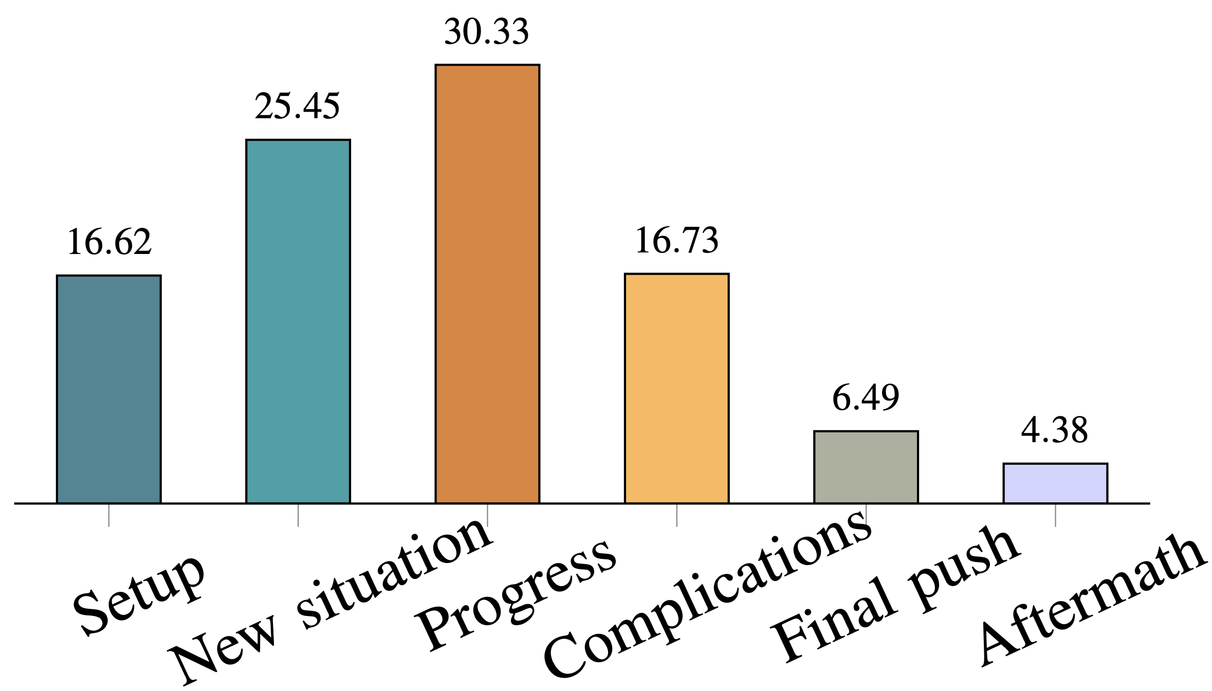
Figure 4: Distribution of trailer shots corresponding to different sections of a movie (development set) as determined by TPs. Trailer shots come from all parts of the movie, even from the end, although the majority are from the beginning and middle.

Opportunity	52.63
Change of plans	55.26
Point of no return	47.37
Major setback	34.21
Climax	34.21

Table 7: Percentage (%) of trailers that include at least one shot labeled as a specific type of TP on the development set. The first two TPs (that present an introduction to the story) appear more frequently in trailers, especially in comparison with the last two, which often contain major spoilers.

	Sentiment intensity
First part	11.50
Second part	9.35
Third part	14.75

Table 8: Average absolute sentiment intensity per trailer section, when we divide the trailers into three even parts (development set).

Step 1 - Initialize path: sample shot from TP1 predictions	Step 2: Select next shot from immediate neighborhood
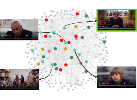
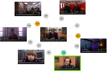
Step 3: Select next shot from immediate neighborhood	Step 4: Select next shot from immediate neighborhood

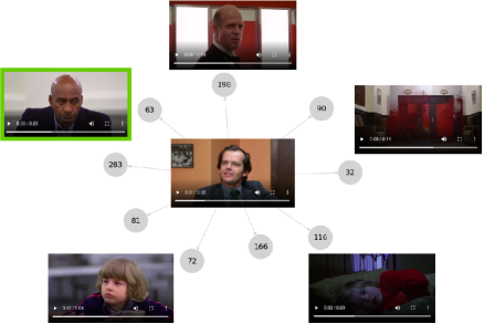
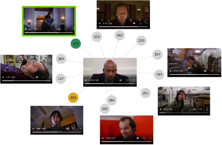
Figure 5: Run of GraphTrailer algorithm for the movie ”The Shining”. Step 1 illustrates the shot-level graph (pruned for better visualization) with colored nodes representing the different types of TPs predicted in the movie (i.e., TP1, TP2, TP3, TP4, TP5). Our algorithm starts by sampling a shot identified as TP1 by VideoGraph (Step 1). For each next step, we only consider the immediate neighborhood of the current shot (i.e., 6–12 neighbors) and select the next shot based on the following criteria: (1) semantic similarity, (2) time proximity, (3) narrative structure, and (4) sentiment intensity (Steps 2-4). Our algorithm continues in Figure 6.

Step 5: Select next shot from immediate neighborhood	Step 6: Select next shot from immediate neighborhood
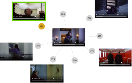
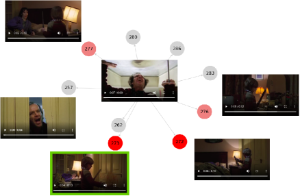
Step 7: Select next shot from immediate neighborhood	Step 8: Create trailer based on retrieved sequence of shots

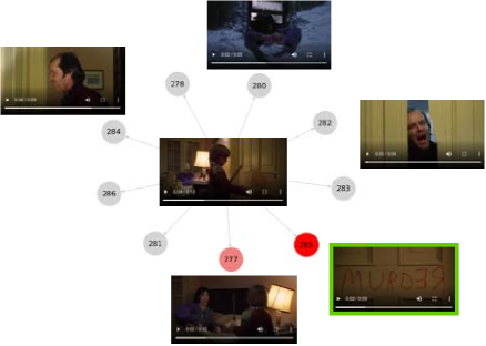
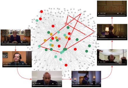
Figure 6: We continue to build the trailer path by selecting the next shot from the immediate neighborhood based on interpretable criteria (Steps 5–7). Finally, we assemble the proposal trailer by concatenating the shots in the path. Our algorithm allows users to review candidate shots at each step and manually select the best one while taking into account our criteria. GraphTrailer allows users to create trailers by only reviewing around 10% of the movie based on recommendations which are interpretable (e.g., coherence with previous shot, relevance to story or intensity).

Appendix D Task Decomposition Analysis

How Narrative Structure Connects with Trailers

According to screenwriting theory [22], the five TPs segment movies into six thematic units, namely, ”Setup”, ”New Situation”, ”Progress”, ”Complications and Higher Stakes”, ”Final Push”, and ”Aftermath”. To examine which parts of the movie are most prevalent in a trailer, we compute the distribution of shots per thematic unit in gold trailers (using the extended development set of TRIPOD). As shown in Figure 4, trailers on average contain shots from all sections of a movie, even from the last two, which might reveal the ending. Moreover, most trailer shots (30.33%) are selected from the middle of the movie (i.e., Progress) as well as from the beginning (i.e., 16.62% and 25.45% for “Setup” and “New Situation”, respectively). These empirical observations corroborate industry principles for trailer creation.

Next, we find how often the trailers include the different types of key events denoted by TPs. We present the percentage of trailers (on the development set) that include at least one shot per TP in Table 7. As can be seen, more than half of the trailers (i.e., 52.63% and 55.26%) include shots related to the first two TPs, whereas only 34.21% of trailers have any information about the two final ones. This is expected, since the first TPs are introductory to the story and hence more important for making trailers, whereas the last two may contain spoilers and are often avoided.

How Sentiment Connects with Trailers

Empirical rules for trailer making suggest that a trailer should start with shots of medium intensity to captivate the viewers, then decrease the sentiment intensity in order to deliver key information about the movie, and finally build up the tension until it reaches a climax.

Here, we analyze the sentiment flow in real trailers from our development set based on predicted sentiment scores (see Sections 3.5 and 4). Specifically, we compute the absolute sentiment intensity (i.e., regardless of positive/negative polarity) per shot in the (true) trailers. In accordance with our experimental setup, we again map trailer shots to movie shots based on visual similarity and consider the corresponding sentiment scores predicted by our network. We then segment the trailer into three equal sections and compute the average absolute sentiment intensity per section. In Table 8 presents the results. As expected, on average, the second part is the least intense, whereas the third has the highest sentiment intensity. Finally, when we again segment each trailer into three equal sections and measure the sentiment flow from one section to the next, we find that 46.67% of the trailers follow a ”V” shape, similar to our sentiment condition for generating proposal trailers with GraphTrailer.

Examples of Walks in GraphTrailer

We present in Figures 5 and 6 a real example of how GraphTrailer operates over a sparse (shot) graph for the movie ”The Shining”. Here, we show the algorithm’s inner workings on a further pruned graph for better visualization (Step 1; Figure 5), while in reality we use the full graph as input to GraphTrailer.

We begin with shots that have been identified as TP1 (i.e., ”Opportunity”; introductory event for the story). We sample a shot (i.e., bright green nodes in graph) and initialize our path. For the next steps (2–7; in reality, we execute up to 10 steps, but we excluded a few for brevity), we only examine the immediate neighborhood of the current node and select the next shot to be included in the path based on the following criteria: (1) semantic coherence, (2) time proximity, (3) narrative structure, and (4) sentiment intensity. We give more details about how we formalize and combine these criteria in Section 3.1.

We observe that our algorithm manages to stay close to important events (colored nodes) while creating the path, which means that we reduce the probability of selecting random shots that are irrelevant to the main story. Finally, in Step 8, Figure 6, we assemble the proposal trailer by concatenating all shots in the retrieved path. We also illustrate the path in the graph (i.e., red line).

An advantage of our approach is that it is interpretable and can be easily used as a tool with a human in the loop. Specifically, given the immediate neighborhood at each step, one could select shots based on different automatic criteria or even manually. Our approach drastically reduces the amount of shots that need to be reviewed to create trailer sequences to 10% of the movie. Moreover, our criteria allow users to explore different sections of the movie, and create diverse trailers.

References

- [1] Muhammad Abdul-Mageed and Lyle Ungar. EmoNet: Fine-grained emotion detection with gated recurrent neural networks. In Proceedings of the 55th Annual Meeting of the Association for Computational Linguistics (Volume 1: Long Papers), pages 718–728, Vancouver, Canada, July 2017. Association for Computational Linguistics.
- [2] Uri Alon and Eran Yahav. On the bottleneck of graph neural networks and its practical implications. In International Conference on Learning Representations, 2020.
- [3] Jimmy Ba and Rich Caruana. Do deep nets really need to be deep? In Proceedings of the Advances in Neural Information Processing Systems, pages 2654–2662, Montreal, Quebec, Canada, 2014.
- [4] AmirAli Bagher Zadeh, Paul Pu Liang, Soujanya Poria, Erik Cambria, and Louis-Philippe Morency. Multimodal language analysis in the wild: CMU-MOSEI dataset and interpretable dynamic fusion graph. In Proceedings of the 56th Annual Meeting of the Association for Computational Linguistics (Volume 1: Long Papers), pages 2236–2246, Melbourne, Australia, July 2018. Association for Computational Linguistics.
- [5] Max Bain, Arsha Nagrani, Andrew Brown, and Andrew Zisserman. Condensed movies: Story based retrieval with contextual embeddings. In Proceedings of the Asian Conference on Computer Vision, 2020.
- [6] Pablo Barceló, Egor V Kostylev, Mikael Monet, Jorge Pérez, Juan Reutter, and Juan Pablo Silva. The logical expressiveness of graph neural networks. In International Conference on Learning Representations, 2019.
- [7] Yoshua Bengio, Nicholas Léonard, and Aaron Courville. Estimating or propagating gradients through stochastic neurons for conditional computation. arXiv preprint arXiv:1308.3432, 2013.
- [8] Sanjay Bilakhia, Stavros Petridis, Anton Nijholt, and Maja Pantic. The MAHNOB mimicry database: A database of naturalistic human interactions. Pattern Recognition Letters, 66:52–61, 2015. Pattern Recognition in Human Computer Interaction.
- [9] Carlos Busso, Murtaza Bulut, Chi-Chun Lee, Abe Kazemzadeh, Emily Mower, Samuel Kim, Jeannette N Chang, Sungbok Lee, and Shrikanth S Narayanan. Iemocap: Interactive emotional dyadic motion capture database. Language resources and evaluation, 42(4):335, 2008.
- [10] Joao Carreira and Andrew Zisserman. Quo vadis, action recognition? a new model and the kinetics dataset. In 2017 IEEE Conference on Computer Vision and Pattern Recognition (CVPR), pages 4724–4733. IEEE Computer Society, 2017.
- [11] Paola Cascante-Bonilla, Kalpathy Sitaraman, Mengjia Luo, and Vicente Ordonez. Moviescope: Large-scale analysis of movies using multiple modalities. arXiv preprint arXiv:1908.03180, 2019.
- [12] Daniel Cer, Yinfei Yang, Sheng-yi Kong, Nan Hua, Nicole Limtiaco, Rhomni St John, Noah Constant, Mario Guajardo-Cespedes, Steve Yuan, Chris Tar, et al. Universal sentence encoder. arXiv preprint arXiv:1803.11175, 2018.
- [13] James E Cutting. Narrative theory and the dynamics of popular movies. Psychonomic Bulletin and review, 23(6):1713–1743, 2016.
- [14] Jia Deng, Wei Dong, Richard Socher, Li-Jia Li, Kai Li, and Li Fei-Fei. Imagenet: A large-scale hierarchical image database. In 2009 IEEE conference on computer vision and pattern recognition, pages 248–255. Ieee, 2009.
- [15] David K Duvenaud, Dougal Maclaurin, Jorge Iparraguirre, Rafael Bombarell, Timothy Hirzel, Alan Aspuru-Guzik, and Ryan P Adams. Convolutional networks on graphs for learning molecular fingerprints. Advances in Neural Information Processing Systems, 28:2224–2232, 2015.
- [16] Jort F Gemmeke, Daniel PW Ellis, Dylan Freedman, Aren Jansen, Wade Lawrence, R Channing Moore, Manoj Plakal, and Marvin Ritter. Audio set: An ontology and human-labeled dataset for audio events. In 2017 IEEE International Conference on Acoustics, Speech and Signal Processing (ICASSP), pages 776–780. IEEE, 2017.
- [17] Deepanway Ghosal, Navonil Majumder, Alexander Gelbukh, Rada Mihalcea, and Soujanya Poria. Cosmic: Commonsense knowledge for emotion identification in conversations. In Proceedings of the 2020 Conference on Empirical Methods in Natural Language Processing: Findings, pages 2470–2481, 2020.
- [18] Ross Girshick. Fast r-cnn. In Proceedings of the IEEE international conference on computer vision, pages 1440–1448, 2015.
- [19] Philip John Gorinski and Mirella Lapata. Movie script summarization as graph-based scene extraction. In Proceedings of the 2015 Conference of the North American Chapter of the Association for Computational Linguistics: Human Language Technologies, pages 1066–1076, Denver, Colorado, May–June 2015. Association for Computational Linguistics.
- [20] Michael Grimm, Kristian Kroschel, and Shrikanth Narayanan. The Vera am Mittag German audio-visual emotional speech database. In ICME, pages 865–868. IEEE, 2008.
- [21] Michael Gutmann and Aapo Hyvärinen. Noise-contrastive estimation: A new estimation principle for unnormalized statistical models. In Proceedings of the Thirteenth International Conference on Artificial Intelligence and Statistics, pages 297–304, 2010.
- [22] Michael Hauge. Storytelling Made Easy: Persuade and Transform Your Audiences, Buyers, and Clients – Simply, Quickly, and Profitably. Indie Books International, 2017.
- [23] Geoffrey Hinton, Oriol Vinyals, and Jeff Dean. Distilling the knowledge in a neural network. arXiv preprint arXiv:1503.02531, 2015.
- [24] Go Irie, Takashi Satou, Akira Kojima, Toshihiko Yamasaki, and Kiyoharu Aizawa. Automatic trailer generation. In Proceedings of the 18th ACM international conference on Multimedia, pages 839–842, 2010.
- [25] Eric Jang, Shixiang Gu, and Ben Poole. Categorical reparametrization with gumble-softmax. In International Conference on Learning Representations (ICLR 2017), 2017.
- [26] Steven Kearnes, Kevin McCloskey, Marc Berndl, Vijay Pande, and Patrick Riley. Molecular graph convolutions: moving beyond fingerprints. Journal of computer-aided molecular design, 30(8):595–608, 2016.
- [27] Hyounghun Kim, Zineng Tang, and Mohit Bansal. Dense-caption matching and frame-selection gating for temporal localization in videoqa. In Proceedings of the 58th Annual Meeting of the Association for Computational Linguistics, pages 4812–4822, 2020.
- [28] Thomas N. Kipf and Max Welling. Semi-supervised classification with graph convolutional networks. In International Conference on Learning Representations (ICLR), 2017.
- [29] Yanran Li, Hui Su, Xiaoyu Shen, Wenjie Li, Ziqiang Cao, and Shuzi Niu. Dailydialog: A manually labelled multi-turn dialogue dataset. In Proceedings of the Eighth International Joint Conference on Natural Language Processing (Volume 1: Long Papers), pages 986–995, 2017.
- [30] David Lopez-Paz, Léon Bottou, Bernhard Schölkopf, and Vladimir Vapnik. Unifying distillation and privileged information. arXiv preprint arXiv:1511.03643, 2015.
- [31] Jordan Louviere, T.N. Flynn, and A. A. J. Marley. Best-worst scaling: Theory, methods and applications. 01 2015.
- [32] Chris J. Maddison, Andriy Mnih, and Yee Whye Teh. The concrete distribution: A continuous relaxation of discrete random variables. In 5th International Conference on Learning Representations, ICLR 2017, Toulon, France, April 24-26, 2017, Conference Track Proceedings, 2017.
- [33] Antoine Miech, Jean-Baptiste Alayrac, Lucas Smaira, Ivan Laptev, Josef Sivic, and Andrew Zisserman. End-to-end learning of visual representations from uncurated instructional videos. In Proceedings of the IEEE/CVF Conference on Computer Vision and Pattern Recognition, pages 9879–9889, 2020.
- [34] Antoine Miech, Dimitri Zhukov, Jean-Baptiste Alayrac, Makarand Tapaswi, Ivan Laptev, and Josef Sivic. Howto100m: Learning a text-video embedding by watching hundred million narrated video clips. In Proceedings of the IEEE/CVF International Conference on Computer Vision, pages 2630–2640, 2019.
- [35] Rada Mihalcea and Paul Tarau. Textrank: Bringing order into text. In Proceedings of the 2004 conference on empirical methods in natural language processing, pages 404–411, 2004.
- [36] Cory S Myers and Lawrence R Rabiner. A comparative study of several dynamic time-warping algorithms for connected-word recognition. Bell System Technical Journal, 60(7):1389–1409, 1981.
- [37] Kenta Oono and Taiji Suzuki. Graph neural networks exponentially lose expressive power for node classification. In International Conference on Learning Representations, 2019.
- [38] Aaron van den Oord, Yazhe Li, and Oriol Vinyals. Representation learning with contrastive predictive coding. arXiv preprint arXiv:1807.03748, 2018.
- [39] Boxiao Pan, Haoye Cai, De-An Huang, Kuan-Hui Lee, Adrien Gaidon, Ehsan Adeli, and Juan Carlos Niebles. Spatio-temporal graph for video captioning with knowledge distillation. In Proceedings of the IEEE/CVF Conference on Computer Vision and Pattern Recognition, pages 10870–10879, 2020.
- [40] Pinelopi Papalampidi, Frank Keller, Lea Frermann, and Mirella Lapata. Screenplay summarization using latent narrative structure. In Proceedings of the 58th Annual Meeting of the Association for Computational Linguistics, pages 1920–1933, 2020.
- [41] Pinelopi Papalampidi, Frank Keller, and Mirella Lapata. Movie plot analysis via turning point identification. In Proceedings of the 2019 Conference on Empirical Methods in Natural Language Processing and the 9th International Joint Conference on Natural Language Processing (EMNLP-IJCNLP), pages 1707–1717, 2019.
- [42] Pinelopi Papalampidi, Frank Keller, and Mirella Lapata. Movie summarization via sparse graph construction. In Thirty-Fifth AAAI Conference on Artificial Intelligence, 2021.
- [43] Soujanya Poria, Devamanyu Hazarika, Navonil Majumder, Gautam Naik, Erik Cambria, and Rada Mihalcea. Meld: A multimodal multi-party dataset for emotion recognition in conversations. In Proceedings of the 57th Annual Meeting of the Association for Computational Linguistics, pages 527–536, 2019.
- [44] Anna Rohrbach, Marcus Rohrbach, Niket Tandon, and Bernt Schiele. A dataset for movie description. In Proceedings of the IEEE conference on computer vision and pattern recognition, pages 3202–3212, 2015.
- [45] Minjoon Seo, Aniruddha Kembhavi, Ali Farhadi, and Hannaneh Hajishirzi. Bidirectional attention flow for machine comprehension. In International Conference on Learning Representations, 2017.
- [46] Alan F Smeaton, Bart Lehane, Noel E O’Connor, Conor Brady, and Gary Craig. Automatically selecting shots for action movie trailers. In Proceedings of the 8th ACM international workshop on Multimedia information retrieval, pages 231–238, 2006.
- [47] John R Smith, Dhiraj Joshi, Benoit Huet, Winston Hsu, and Jozef Cota. Harnessing ai for augmenting creativity: Application to movie trailer creation. In Proceedings of the 25th ACM international conference on Multimedia, pages 1799–1808, 2017.
- [48] Siqi Sun, Zhe Gan, Yuwei Fang, Yu Cheng, Shuohang Wang, and Jingjing Liu. Contrastive distillation on intermediate representations for language model compression. In Proceedings of the 2020 Conference on Empirical Methods in Natural Language Processing (EMNLP), pages 498–508, 2020.
- [49] Makarand Tapaswi, Martin Bauml, and Rainer Stiefelhagen. Book2movie: Aligning video scenes with book chapters. In Proceedings of the IEEE Conference on Computer Vision and Pattern Recognition, pages 1827–1835, 2015.
- [50] Makarand Tapaswi, Yukun Zhu, Rainer Stiefelhagen, Antonio Torralba, Raquel Urtasun, and Sanja Fidler. Movieqa: Understanding stories in movies through question-answering. In Proceedings of the IEEE conference on computer vision and pattern recognition, pages 4631–4640, 2016.
- [51] Kristin Thompson. Storytelling in the new Hollywood: Understanding classical narrative technique. Harvard University Press, 1999.
- [52] Ashish Vaswani, Noam Shazeer, Niki Parmar, Jakob Uszkoreit, Llion Jones, Aidan N Gomez, Łukasz Kaiser, and Illia Polosukhin. Attention is all you need. In Advances in neural information processing systems, pages 5998–6008, 2017.
- [53] Lezi Wang, Dong Liu, Rohit Puri, and Dimitris N Metaxas. Learning trailer moments in full-length movies with co-contrastive attention. In European Conference on Computer Vision, pages 300–316. Springer, 2020.
- [54] Yuxin Wu, Alexander Kirillov, Francisco Massa, Wan-Yen Lo, and Ross Girshick. Detectron2. https://github.com/facebookresearch/detectron2, 2019.
- [55] Zhirong Wu, Yuanjun Xiong, Stella X Yu, and Dahua Lin. Unsupervised feature learning via non-parametric instance discrimination. In Proceedings of the IEEE Conference on Computer Vision and Pattern Recognition, pages 3733–3742, 2018.
- [56] Saining Xie, Ross Girshick, Piotr Dollár, Zhuowen Tu, and Kaiming He. Aggregated residual transformations for deep neural networks. In Proceedings of the IEEE conference on computer vision and pattern recognition, pages 1492–1500, 2017.
- [57] Hongteng Xu, Yi Zhen, and Hongyuan Zha. Trailer generation via a point process-based visual attractiveness model. In Proceedings of the 24th International Conference on Artificial Intelligence, pages 2198–2204, 2015.