Stronger Generalization Guarantees for Robot Learning by
Combining Generative Models and Real-World Data

Abstract

We are motivated by the problem of learning policies for robotic systems with rich sensory inputs (e.g., vision) in a manner that allows us to guarantee generalization to environments unseen during training. We provide a framework for providing such generalization guarantees by leveraging a finite dataset of real-world environments in combination with a (potentially inaccurate) generative model of environments. The key idea behind our approach is to utilize the generative model in order to implicitly specify a prior over policies. This prior is updated using the real-world dataset of environments by minimizing an upper bound on the expected cost across novel environments derived via Probably Approximately Correct (PAC)-Bayes generalization theory. We demonstrate our approach on two simulated systems with nonlinear/hybrid dynamics and rich sensing modalities: (i) quadrotor navigation with an onboard vision sensor, and (ii) grasping objects using a depth sensor. Comparisons with prior work demonstrate the ability of our approach to obtain stronger generalization guarantees by utilizing generative models. We also present hardware experiments for validating our bounds for the grasping task.

I Introduction

The ability of modern deep learning techniques to process high-dimensional sensory inputs (e.g., vision or depth) provides a promising avenue for training autonomous robotic systems such as drones, robotic manipulators, or autonomous vehicles to operate in complex and real-world environments. However, one of the fundamental challenges with current learning-based approaches for controlling robots is their limited ability to generalize beyond the specific set of environments they are trained on [1]. This lack of generalization is a particularly pressing problem for safety- or performance-critical systems for which one would ideally like to provide formal guarantees on generalization to novel environments.

A primary contributing factor to this challenge is the fact that real-world datasets for training robotic systems are often limited in size (e.g., in comparison to large-scale datasets available for training visual recognition models via supervised learning). Such datasets often have to be carefully and painstakingly curated, e.g., by scanning indoor environments using 3D cameras for creating a dataset for visual navigation tasks [2, 3, 4], or scanning objects and characterizing their physical properties (e.g., inertia, friction, and mass) for creating a dataset for robotic manipulation [5, 6, 7]. One way to address this challenge of scarce real-world data is to leverage data from a generative model of environments. As an example, consider the problem of manipulating mugs (Fig. 1); one could hand-craft a generative model that produces shapes that are similar to mugs (e.g., hollow cylinders; Fig. 1) or potentially train a generative model over shapes using a dataset of different objects (e.g., bowls).

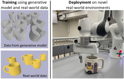
Figure 1: A schematic of our overall approach. We provide a framework for providing generalization guarantees on novel environments by combining a (potentially inaccurate) generative model of environments (e.g., a distribution that generates hollow cylinders) with a finite dataset of real-world environments (e.g., a datset of mugs). We validate our approach on hardware using the Franka Panda arm, and through multiple simulation experiments.

The two sources of data outlined above have complementary features: real-world data is scarce but representative, while data from a generative model is plentiful but potentially different from environments the robot will encounter when deployed. Thus, relying entirely on the small real-world dataset can pose the risk of overfitting, while relying entirely on the generative model may cause the robot to overfit to the specific features of this model and prevent generalization to real-world environments. How can we effectively combine these two sources in order to guarantee that the robot will generalize to novel real-world environments?

Statement of contributions: We provide a framework for providing formal guarantees on generalization to novel environments for robotic systems with rich sensory inputs by leveraging a combination of finite real-world data and a (potentially inaccurate) generative model of environments. To our knowledge, the approach presented here is the first to leverage these two sources of data while providing generalization guarantees for robotic systems. The key technical insight behind our approach is to utilize the generative model for specifying a prior over control policies. In order to achieve this, we develop a technique for implicitly parameterizing policies via datasets of environments. We then train a posterior distribution over policies using the real-world dataset; this posterior is trained to minimize an upper bound on the expected cost across novel environments derived via Probably Approximately Correct (PAC)-Bayes generalization theory. Minimizing the PAC-Bayes bound allows us to automatically trade-off reliance on the real-world dataset and the generative model, while resulting in policies with a guaranteed bound on expected performance in novel environments. We demonstrate our approach on two examples which use vision inputs: (i) navigation of an unmanned aerial vehicle (UAV) through obstacle fields, and (ii) grasping of mugs by a robotic manipulator. For both examples, we obtain PAC-Bayes bounds that guarantee successful completion of the task in 80–95% of novel environments. Comparisons with prior work demonstrate the ability of our approach to obtain stronger generalization guarantees by utilizing generative models. We also present hardware experiments for validating our bounds on the grasping task.

I-A Related Work

Domain randomization and data augmentation. Domain randomization (DR) is a popular technique for improving the generalization of policies learned via reinforcement learning (RL). DR generates new training environments by randomizing specified dynamics and environmental parameters, e.g., object textures, friction properties, and lighting conditions [8, 9, 10, 11, 12], or generating new objects for manipulation by combining different shape primitives [13]. Similarly, data augmentation techniques such as random cutout and cropping [14, 15] seek to improve generalization for vision-based RL tasks by performing transformations on the observation space. While these techniques have been empirically shown to improve generalization, they do not provide any guarantees on generalization (which is the focus of our work).

Generative modeling of environments. Domain randomization techniques do not necessarily generate realistic environments for training. Consequently, another line of work seeks to address this challenge by generating environments with more realistic structure, e.g., via scene grammars and variational inference [16, 17, 18], procedural generation [19], or evolutionary algorithms [20]. Adversarial techniques have also been developed for generating challenging environments [21, 22]. Prior work has also explored augmenting real-world training with large amounts of procedurally generated environments via domain adaptation techniques [23], transfer learning [24], or fine-tuning [25]. We highlight that none of the methods above provide guarantees on generalization to real-world environments. In this work, we provide a framework based on PAC-Bayes generalization theory in order to combine environments from a generative model with real-world environments and provide generalization guarantees for the resulting policies. Our work is thus complementary to the above techniques and could potentially leverage advances in generative modeling.

Generalization theory. Generalization theory provides a framework for learning hypotheses (in supervised learning) with guaranteed bounds on the true expected loss on new examples drawn from the underlying (but unknown) data-generating distribution, given only a finite number of training examples. Early frameworks include Vapnik-Chervonenkis (VC) theory [26] and Rademacher complexity [27]. However, these methods often provide vacuous generalization bounds for high-dimensional hypothesis spaces (e.g., neural networks). Bounds based on PAC-Bayes generalization theory [28, 29, 30] have recently been shown to provide strong generalization guarantees for neural networks in a variety of supervised learning settings [31, 32, 33, 34, 35, 36], and have been significantly extended and improved [37, 38, 39, 40, 41, 42]. PAC-Bayes has also recently been extended to learn policies for robots with guarantees on generalization to novel environments [43, 44, 45, 46]. In this paper, we build on this work and provide a framework for leveraging generative models as a form of prior knowledge within PAC-Bayes. Comparisons with the approaches presented in [44, 45] demonstrate that this leads to stronger generalization guarantees and empirical performance (see Section V for numerical results).

II Problem Formulation

Dynamics, environments, and sensing. Consider a robotic system with discrete-time dynamics given by:

$$x_{t+1}=f_{E}(x_{t},u_{t}),$$ (1)

where $x_{t}\in$ $\mathcal{X}\subseteq\mathbb{R}^{n_{x}}$ is the state of the robot at time-step $t$, $u_{t}\in\mathcal{U}\subseteq\mathbb{R}^{n_{u}}$ is the control input, and $E\in\mathcal{E}$ is the environment that the robot is operating in. The term “environment” is used broadly to represent all external factors which influence the evolution of the state of the robot, e.g., an obstacle field that a UAV has to avoid, external disturbances such as wind gusts, or an object that a robotic manipulator is grasping. The dynamics of the robot may be nonlinear/hybrid. Let $\mathcal{O}\subseteq\mathbb{R}^{n_{o}}$ denote the space corresponding to the robot’s sensor observations (e.g., the space of images for a camera).

Policies and cost functions. Let $\pi:\mathcal{O}\rightarrow\mathcal{U}$ be a policy that maps observations (or potentially a history of observations) to actions, and let $\Pi$ denote the space of policies (e.g., neural networks with a certain architecture). The robot’s task is specified via a cost function; we let $C_{E}(\pi)$ denote the cost incurred by policy $\pi$ when deployed in environment $E$ over a time horizon $T$. As an example in the context of UAV navigation, the cost function can assign 1 if the UAV collides with an obstacle, or 0 if it successfully reaches its goal. We assume that the cost is bounded, and without further loss of generality assume that $C_{E}(\pi)\in[0,1]$. Importantly, we make no further assumptions on the cost function (e.g., we do not assume continuity or Lipschitzness).

Dataset of real-world environments. We assume that there is an underlying distribution $\mathcal{D}$ from which real-world environments that the robot operates in are drawn (e.g., an underlying distribution over obstacle environments for UAV navigation, or objects for grasping). Importantly, we do not assume that we have explicit knowledge of $\mathcal{D}$ or the space $\mathcal{E}$ of real-world environments. Instead, we assume access to a finite dataset $S:=\{E_{1},E_{2},...,E_{N}\}$ of $N$ real-world environments drawn independently from $\mathcal{D}$.

Generative model. In addition to the (potentially small) dataset of real-world environments, we assume access to a generative model over environments. This generative model takes the form of a distribution $\mathcal{D}_{\text{gen}}$ over a space $\mathcal{E}_{\text{gen}}$ of environments. Importantly, $\mathcal{D}_{\text{gen}}\neq\mathcal{D}$ and $\mathcal{E}_{\text{gen}}\neq\mathcal{E}$ in general. Indeed, the space $\mathcal{E}_{\text{gen}}$ will typically be significantly simpler than the space $\mathcal{E}$ of real-world environments. For example, in the context of manipulation (Fig. 1), $\mathcal{E}$ may correspond to the space of all mugs while $\mathcal{E}_{\text{gen}}$ may correspond to the space of hollow cylinders (described by a small number of geometric and physical parameters).

Goal. Our goal is to learn a policy that provably generalizes to novel real-world environments drawn from $\mathcal{D}$. In this paper, we will employ a slightly more general formulation where we choose a distribution $P$ over policies (instead of choosing a single policy). This allows for the use of PAC-Bayes generalization theory. Our goal is then to tackle the following optimization problem:

$$\min_{P\in\mathcal{P}}\ C_{\mathcal{D}}(P),\ \text{where}\ C_{\mathcal{D}}(P):=\mathop{\mathbb{E}}_{E\sim\mathcal{D}}\mathop{\mathbb{E}}_{\pi\sim P}[C(\pi;E)].$$ (2)

The primary challenge in tackling this problem is that the distribution $\mathcal{D}$ is unknown to us. Instead, we have access to a finite number of real-world environments and a (potentially inaccurate) generative model. In the next section, we describe how to leverage these two sources of data in order to learn a distribution $P$ over policies with a guaranteed bound on the expected cost $C_{\mathcal{D}}(P)$, i.e., a provable guarantee on generalization to novel environments drawn from $\mathcal{D}$.

III Generalization Guarantees with
Generative Models

In this section, we describe how to combine generative models with a finite amount of real data in order to produce strong generalization guarantees via PAC-Bayes theory.

III-A PAC-Bayes Control

Our objective is to solve the optimization problem (2). However, the lack of an explicit characterization of $\mathcal{D}$ prohibits us from directly minimizing $C_{\mathcal{D}}(P)$. PAC-Bayes generalization bounds [29] provide a high-confidence upper bound on $C_{\mathcal{D}}(P)$ in terms of the empirical cost on the training environments $S$ that are drawn from $\mathcal{D}$ and a regularizer. As both these terms can be computed, we minimize the PAC-Bayes upper bound in order to indirectly minimize $C_{\mathcal{D}}(P)$. Additionally, the PAC-Bayes bound serves as a certificate of generalization to novel environments drawn from $\mathcal{D}$.

Let $\Pi:=\{\pi_{\theta}\leavevmode\nobreak\ |\leavevmode\nobreak\ \theta\in\Theta\subseteq\mathbb{R}^{n_{\theta}}\}$ denote the space of policies parameterized by the vector $\theta$; as an example, $\theta$ could be the weights and biases of a neural network. For a “posterior” policy distribution $P$ on $\Pi$ and a real-world dataset $S\coloneqq\{E_{1},E_{2},\cdots,E_{N}\}$ of $N$ environments drawn i.i.d from $\mathcal{D}$, we define the empirical cost as the expected cost across the environments in $S$:

$$C_{S}(P)\coloneqq\frac{1}{N}\sum_{E\in S}\mathop{\mathbb{E}}_{\theta\sim P}[C(\pi_{\theta},E)].$$ (3)

Let $P_{0}$ be a “prior” distribution over $\Pi$ which is specified before the training dataset $S$ is observed. The PAC-Bayes theorem below then provides an upper bound on the true expected cost $C_{\mathcal{D}}(P)$ which holds with high probability.

Theorem 1 (adapted from [44]).

For any $\delta\in(0,1)$ and posterior $P$, with probability at least $1-\delta$ over sampled environments $S\sim\mathcal{D}^{N}$, the following inequality holds:

$$\leavevmode\nobreak\ C_{\mathcal{D}}(P) \leq C_{PAC}(P,P_{0})$$

$$:=\big{(}\sqrt{C_{S}(P)+R(P,P_{0})}+\sqrt{R(P,P_{0})}\big{)}^{2},$$ (4)

where $R(P,P_{0})$ is a regularization term defined as:

$$R(P,P_{0}):=\frac{\textrm{KL}(P||P_{0})+\log\big{(}\frac{2\sqrt{N}}{\delta}\big{)}}{2N}\enspace.$$ (5)

It is challenging to specify good priors $P_{0}$ on the policy space $\Pi$ in general (e.g., specifying a prior on neural network weights); our previous approaches resorted to techniques such as data splitting [44] and imitation learning [45] to obtain priors. On the other hand, generative models offer an intuitive approach for embedding prior domain knowledge in learning [1, 16, 17, 18, 19]. Motivated by this, we will leverage generative models (based on inductive bias or other data) as priors for the PAC-Bayes theorem.

III-B Policy Parameterization With Datasets

The posterior $P$ and the prior $P_{0}$ distributions in Theorem 1 are on the space $\Pi$ of policies. Our key idea for leveraging generative models to provide generalization guarantees is to provide an approach for implicitly parameterizing policies $\pi_{\theta}$ via synthetic datasets drawn from the generative model. This parameterization is then used in Theorem 1 such that the PAC-Bayes bound is specified in terms of the posterior $Q$ and the prior $Q_{0}$ on the space $\mathcal{E}_{\text{gen}}$ of synthetic environments. Let $\hat{S}$ be a synthetic (i.e., generated) dataset of cardinality $l$ and let $L:\Pi\times\mathcal{E}_{\text{gen}}^{l}\to[0,\infty)$ be a loss function; e.g., $L$ can be the average cost of deploying a policy $\pi_{\theta}$ in environments in $\hat{S}$. Then, let $A:\mathcal{E}_{\text{gen}}^{l}\to\Theta$ be an arbitrary deterministic algorithm for (approximately) solving the optimization problem:

$$\arg\inf_{\theta\in\Theta}L(\pi_{\theta},\hat{S})\enspace.$$ (6)

Any such algorithm then provides a way to parameterize policies $\pi_{A(\hat{S})}$ implicitly via datasets $\hat{S}$. We note that we do not impose any additional conditions on $A$ (e.g., $A$ need not solve (6) to global/local optimality). Moreover, although we require $A$ to be deterministic, we can use stochastic optimization approaches — such as stochastic gradient descent — by fixing a random seed (this ensures deterministic outputs for a given input). The algorithm $A$ gives rise to a push-forward measure for distributions from the synthetic environment space $\mathcal{E}_{\text{gen}}$ to the policy space $\Pi$. We overload the notation to express the push-forward distribution on the policy space as $A(Q)$.

III-C PAC-Bayes Bounds With Generative Models

In order to provide PAC-Bayes bounds using generative models, we encode the posterior $P$ and the prior $P_{0}$ on the policy space via posterior $Q$ and prior $Q_{0}$ generative models as follows: $P=A(Q)$, and $P_{0}=A(Q_{0})$. We are now ready to present the PAC-Bayes bound with generative models.

Theorem 2.

Let $A$ be a deterministic algorithm as defined above. For any $\delta\in(0,1)$ and posterior generative model $Q$ on $\mathcal{E}_{\text{gen}}$, with probability at least $1-\delta$ over sampled real-world environments $S\sim\mathcal{D}^{N}$, the following holds:

$$\leavevmode\nobreak\ C_{\mathcal{D}}(A(Q)) \leq C_{PAC}(Q,Q_{0})$$

$$:=\big{(}\sqrt{C_{S}(A(Q))+R(Q,Q_{0})}+\sqrt{R(Q,Q_{0})}\big{)}^{2},$$ (7)

where

$$C_{S}(A(Q)):=\frac{1}{N}\sum_{E\in S}\mathop{\mathbb{E}}_{\hat{S}\sim Q}[C(\pi_{A(\hat{S})},E)]$$ (8)

and $R(Q,Q_{0})$ is the same as (5).

Proof.

The proof follows by choosing $A(Q)$ as the posterior policy distribution $P$ and $A(Q_{0})$ as the prior policy distribution $P_{0}$ in (4), giving us the following bound:

$$C_{\mathcal{D}}(A(Q)) \leq\big{(}\sqrt{C_{S}(A(Q))+R(A(Q),A(Q_{0}))}$$ (9)

$$\phantom{\leq}+\sqrt{R(A(Q),A(Q_{0}))}\big{)}^{2},$$ (10)

The empirical cost can be expressed as:

$$C_{S}(A(Q))=\frac{1}{N}\sum_{E\in S}\mathop{\mathbb{E}}_{\theta\sim A(Q)}[C(\pi_{\theta},E)].$$ (11)

Sampling $\theta$ from the push-forward measure $A(Q)$ is equivalent to sampling $\hat{S}$ from $Q$ and then computing $A(\hat{S})$. Therefore, the empirical cost can be expressed as (8).

Using the data processing inequality [47] we have $KL(A(Q)||A(Q_{0}))\leq KL(Q||Q_{0})$, which further results in $R(A(Q),A(Q_{0}))\leq R(Q,Q_{0})$. Using this in (10) completes the proof. ∎

Minimizing $C_{PAC}$ provides us a policy distribution $A(Q)$ with a guaranteed bound on the expected cost $C_{\mathcal{D}}$ on novel environments, thereby tackling the optimization problem (2).

IV Training

In this section, we present our training pipeline for combining a generative model with real-world data in order to provide strong generalization guarantees. First, we describe the algorithm $A$ used for parameterizing policies through datasets (Sec. III-B). Then we provide the algorithm for minimizing the PAC-Bayes upper bound in Theorem 2.

IV-A Policy Parameterization With Datasets

As discussed in Sec. III-B, we require a deterministic algorithm $A$ (that attempts to minimize a loss $L$) in order to implicitly parameterize policies $\pi_{A(\hat{S})}$ via datasets $\hat{S}$. For the results in this paper, we use $L$ as the average cost of deploying a policy $\pi_{\theta}$ in environments contained in $\hat{S}$:

$$L(\pi_{\theta},\hat{S}):=\frac{1}{l}\sum_{E_{\text{gen}}\in\hat{S}}C(\pi_{\theta},E_{\text{gen}}).$$ (12)

To minimize $L$, we choose the algorithm $A$ to be Evolutionary Strategies (ES) [48] with an a priori fixed random seed; fixing the random seed ensures that the algorithm is deterministic. ES belongs to a family of black-box optimizers which train a distribution on the policy space. The choice of ES is driven by our use of black-box simulators through which the gradient of the loss cannot be backpropagated (e.g., due to the loss being non-differentiable or due to the dynamics of the robot being hybrid). Additionally, ES permits a high degree of parallelization, thereby allowing us to effectively exploit clouding computing resources. In the interest of space, further details on our implementation of ES are not provided here and can be found in [44, Sec. 4.1].

IV-B Training a PAC-Bayes Generative Model

We assume availability of a generative model expressed by a distribution $\mathcal{D}_{\text{gen}}$ on $\mathcal{E}_{\text{gen}}$ (ref. Sec. II); this model could be hand-specified based on prior knowledge or constructed using other data. Leveraging $\mathcal{D}_{\text{gen}}$ we first construct a prior generative model and then train a posterior generative model by minimizing the PAC-Bayes bound in Theorem 2.

As has been shown in [44] and [46], PAC-Bayes minimization takes the form of an efficiently-solvable convex program for discrete probability distributions. To exploit this convex formulation (which allows one to optimize the PAC-Bayes bound in a computationally efficient manner), we construct a prior generative model $q_{0}$ which approximates $\mathcal{D}_{\text{gen}}$ as a discrete probability distribution as follows:
Let $\mathcal{D}_{\text{gen}}$ be a generative model which takes the form of a distribution on the synthetic environment space $\mathcal{E}_{\text{gen}}$, as discussed in Sec. II. Sample $m$ datasets of cardinality $l$ each from $\mathcal{D}_{\text{gen}}$ to construct the set of datasets $\tilde{S}:=\{\hat{S}_{1},\cdots,\hat{S}_{m}\leavevmode\nobreak\ |\leavevmode\nobreak\ \hat{S}_{i}\sim\mathcal{D}_{\text{gen}}^{l}\}$. The prior generative model $q_{0}$ is then defined as the uniform distribution on $\hat{S}$.

To train a posterior generative model $q$ (which is a discrete probability distribution on the set $\tilde{S}$ of synthetic datasets), we minimize the PAC-Bayes upper bound in Theorem 2. To transform this minimization into a convex program, we first compute a cost vector $C\in\mathbb{R}^{m}$. Each entry $C_{i}$ of this vector corresponds to the expected cost of deploying the policy $\pi_{A(\hat{S}_{i})}$, parameterized by the synthetic dataset $\hat{S}_{i}$, in the real-world training dataset $S$. Therefore, the empirical cost $C_{S}(A(Q))$ can be expressed as $Cq$ (which is linear in the generative model posterior $q$). Leveraging this, we can express the PAC-Bayes bound minimization as follows:

$$\min_{q\in\mathbb{R}^{m}}\quad \big{(}\sqrt{Cq+R(q,q_{0})}+\sqrt{R(q,q_{0})}\big{)}^{2}$$ (13)

s.t. $$\sum_{i=1}^{m}q_{i}=1,0\leq q_{i}\leq 1.$$

Using the epigraph trick, as detailed in [44], (13) can be further transformed to a convex program. In the interest of space, we direct the reader to [44, Sec. 4.2] for complete details of the algorithm to solve (13). We provide a sketch of our entire training pipeline in Alg. 1.

Algorithm 1 Training Pipeline

1:Input: Generative model: $\mathcal{D}_{\text{gen}}$; real-world dataset: $S\sim\mathcal{D}^{N}$

2:Input: Number of synthetic datasets: $m$

3:Input: Cardinality of each synthetic dataset: $l$

4:Input: Deterministic algorithm for (6): $A$

5:Sample $\hat{S}_{1},\cdots,\hat{S}_{m}\sim\mathcal{D}_{\text{gen}}^{l}$

6:$q_{0}\leftarrow[1/m,\cdots,1/m]$

7:$q\leftarrow\text{PAC-Bayes}(S,A,q_{0},\{\hat{S}_{i}\}_{i=1}^{m})$ by solving (13)

8:return $q$

V Examples

We demonstrate the ability of our framework to provide strong generalization guarantees for two robotic systems with nonlinear/hybrid dynamics and rich sensory inputs: a drone navigating obstacle fields using onboard vision, and a manipulator grasping mugs using an external depth camera. All training is conducted on a Lambda Blade server with 2x Intel Xeon Gold 5220R (96 threads), 760 GB of RAM, and 8 NVIDIA GeForce RTX 2080, each with 12 GB memory. We compare our bounds against those in previous works with similar examples.

V-A Vision-based obstacle avoidance with a drone

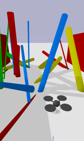
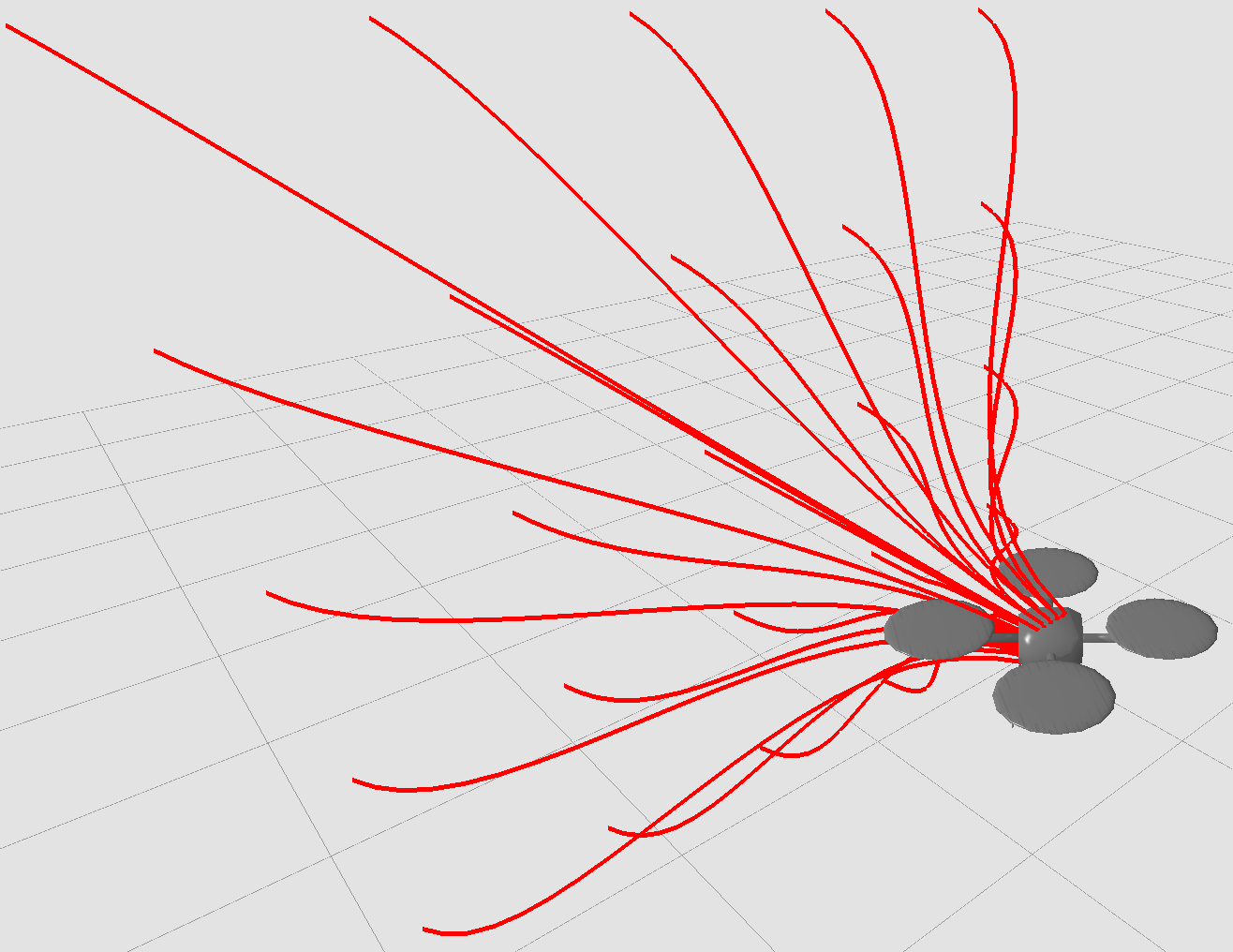
Figure 2: Vision-based navigation with a UAV. (a) Environment with randomly generated obstacles. (b) Primitive library for the UAV.

Overview. In this example, we train a quadrotor equipped with an onboard depth camera to navigate across obstacle fields. The obstacle course is a tunnel populated by cylindrical obstacles as shown in Fig. 2. The dynamics and sensor are simulated using PyBullet [49].

Environments. The distribution $\mathcal{D}$ over environments samples the radii, locations, and orientations of 23 obstacles in order to generate an environment; the radii are drawn from a uniform distribution over [5cm, 30cm], the locations of the center of the cylinders are drawn from [-5m, 5m]$\times$[0m, 14m], and the orientations are quaternion vectors drawn from a normal distribution.

Generative model. The generative model $\mathcal{D_{\rm gen}}$ samples radii, locations, and orientations of obstacles from the same distributions as $\mathcal{D}$. However, the number of obstacles in each environment drawn from $\mathcal{D_{\rm gen}}$ is different from the number of obstacles in environments drawn from $\mathcal{D}$. In our experiments, we will study the effects of degrading the quality of the generative model by varying this parameter.

Motion primitives and planning policy. We pre-compute a library of 25 motion primitives (Fig. 2), each of which is generated by connecting the initial position of the robot to a desired final position by a smooth sigmoidal trajectory. The robot’s policy takes a $50\times 50$ depth image from the onboard camera as input and selects a motion primitive to execute. This policy is applied in a receding-horizon manner (i.e., the robot selects a primitive, executes it, selects another primitive, etc.). The policy is parameterized using a deep neural network ($\sim$14K parameters) and is based on the policy architecture presented in [44, Sec. 5.1].

Training. We choose the cost $1-\frac{k}{K}$ where $k$ is the number of motion primitives successfully executed before colliding with an obstacle and $K$ is the total possible primitive executions; in our example $K=12$. We train policies via the pipeline described in Section IV. We choose $m=50$ datasets in $\tilde{S}$, and each dataset $\hat{S}_{i}\in\tilde{S}$ has cardinality $l=50$. With 6 GPUs and 48 CPUs, it takes $\sim$ 6-8 hours to train the priors and $\sim$ 200-1000 seconds to train the posterior (depending on the number of real environments used).

Results. We consider different generative models $\mathcal{D}_{\text{gen}}$ by varying the number of obstacles $N_{\text{O}}$ sampled in any generated environment; we vary this parameter in the set $\{10,15,20,23,25,30\}$. Generalization guarantees are obtained using each variation of the generative model. We set $\delta=0.01$ to have bounds that hold with probability 0.99.

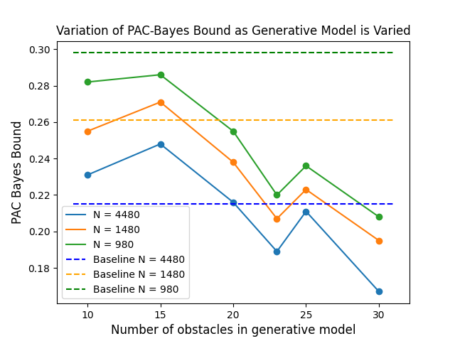
Figure 3: PAC-Bayes bounds for different choices of the generative model (obtained by varying the number $N_{\text{O}}$ of obstacles sampled in each environment). Bounds generally become stronger as we increase $N_{\text{O}}$. Comparisons with [44] (dotted lines) demonstrate the benefits of our approach, particularly for smaller values of $N$ (the number of available real-world environments).

Envs (N) Using generative model (ours) Approach from [44] PAC Bound True Cost (Estimate) PAC Bound True Cost (Estimate) 980 20.92 % 13.81 % 29.82 % 19.7 % 1480 19.60 % 13.81 % 26.02 % 18.34 % 4480 16.76 % 13.86 % 21.52 % 18.43 %

Table I: Comparison of PAC-Bayes bounds with true expected cost on novel environments (estimated via exhaustive sampling). The framework presented here provides both stronger guarantees and empirical performance on novel environments as compared to [44].

Figure 3 plots the PAC-Bayes bounds on the expected cost for different choices of $N_{\text{O}}$. For example, when $N_{\text{O}}=30$ and $N=4480$, the PAC-Bayes bound using our approach is $0.1676$. Thus, we can guarantee that on average the quadrotor will successfully navigate through at least 83.24% ($100\%-16.76\%$) of novel real-world environments. We also compare these bounds with those provided by the method in [44] (plotted with dotted lines), which splits a given dataset of $N$ real-world environments into two portions; the first portion is used to train a prior over policies and the second portion is used to obtain a posterior distribution over policies by minimizing the PAC-Bayes bound in Theorem 1. We provide our approach with the same number of real-world environments (i.e., $N$) as used in [44] in order to ensure a fair comparison. For each $N$, the bounds generally become stronger as we increase the number of obstacles $N_{\text{O}}$ sampled by the generative model.

Figure 3 demonstrates that the approach presented here is able to produce stronger bounds than the ones provided by [44], with significant differences when $N_{\text{O}}=30$. Interestingly, the benefits of our approach become more apparent when the number $N$ of available real-world environments is small. For example, when $N=980$, the bounds provided by our approach are stronger for all choices of $N_{\text{O}}$. When $N$ is small, the prior information provided by the generative model becomes important (as one would intuitively expect).

Table I compares the theoretical generalization bounds obtained for the case when $N_{\text{O}}=30$ with the true expected cost on novel environments (estimated via exhaustive sampling of novel environments). Results are presented for different numbers $N$ of real-world environments for both our method and the one from [44]. As the table illustrates, our approach results in significantly improved performance on novel environments for all values of $N$.

V-B Grasping a diverse set of mugs

Overview. This example aims to train a Franka Panda arm to grasp and lift a mug (Fig. 1). The arm has an overhead camera which provides a 128 $\times$ 128 depth image. The simulation environment for this system is implemented using PyBullet [49], and we also present hardware results on the Franka arm shown in Fig. 1 (right).

Environments. The real-world environments used for training are drawn from a set of mugs with diverse shapes and sizes collected from the ShapeNet dataset [7]. The initial x-y position of these mugs is sampled from the uniform distribution over $[0.45\leavevmode\nobreak\ \text{cm},\leavevmode\nobreak\ 0.55\leavevmode\nobreak\ \text{cm}]\times[-0.05\leavevmode\nobreak\ \text{cm},\leavevmode\nobreak\ 0.05\leavevmode\nobreak\ \text{cm}]$, and yaw orientations are sampled from the uniform distribution over $[-\pi\leavevmode\nobreak\ \text{rad},\pi\leavevmode\nobreak\ \text{rad}]$. All mugs are placed upright.

Generative model. The generative model $\mathcal{D_{\rm gen}}$ comprises of hollow cylinders which are generated using trimesh [50]. The inner radii, outer radii, and height of the cylinders are sampled from uniform distributions. The ratio of the maximum possible outer radius to inner radius is 2, and the height ranges from twice the maximum inner radius to twice the maximum outer radius. The initial location and yaw are sampled from the same distributions as $\mathcal{D}$.

Policy. The robot’s policy is parameterized using a deep neural network (DNN) which takes a depth map of an object and a latent state $z\in\mathbb{R}^{10}$ sampled from a Gaussian distribution as input and outputs a grasp location and orientation. We keep the weights of the DNN fixed and update the distribution on the latent space. Effectively, the latent space acts as the space of policy parameters $\Theta$ and the Gaussian distribution on it is the policy distribution $P$; further details of the policy’s architecture can be found in [45].

Training. If the arm is able to grasp and lift a mug by 10 cm, we consider the rollout to be successful and assign a cost of 0, otherwise we assign a cost of 1. We follow the pipeline in Alg. 1 for training. We choose m = 50 datasets in $\tilde{S}$, with each dataset $\tilde{S}_{i}$ $\in$ $\tilde{S}$ having cardinality l = 50. With 80 CPUs, the priors train in $\sim$ 3 hours, and the posterior takes $\sim$ 900 seconds.

Simulation results. We obtain theoretical generalization guarantees using the generative model described above and compare it with the theoretical guarantees obtained in [45]. We use the same set of 500 mugs from ShapeNet used by [45] as our real dataset in order to train the posterior and obtain the PAC-Bayes bound. Our resulting PAC-Bayes bound (with $\delta=0.99$) is 0.054. Thus, our policy is guaranteed to have a success rate of at least 94.6 %, which is higher than the 93 % guaranteed success rate in [45] (despite using the same real-world dataset of mugs for training).

Hardware results. The posterior policy distribution trained in simulation is deployed on the hardware setup shown in Fig. 1 without additional training (i.e., zero-shot sim-to-real transfer). 10 mugs with diverse shapes are used (Fig. 4). Among three sets of experiments with different seeds (for sampling the latent $z$), the success rates are 100% (10/10), 100% (10/10), and 90% (9/10). The overall success rate is 96.67% (29/30) and thus validates the PAC-Bayes bound of $94.6\%$ trained in simulation.

Figure 4: Mugs used for hardware validation of the grasping policy.

VI Conclusions and Future Work

We have presented an approach for learning policies for robotic systems with guarantees on generalization to novel environments by leveraging a finite dataset of real-world environments in combination with a (potentially inaccurate) generative model of environments. The key idea behind our approach is to use the generative model in order to implicitly specify a prior over policies, which is then updated using the real-world environments by optimizing generalization bounds derived via PAC-Bayes theory. Our simulation and hardware results demonstrate the ability of our approach to provide strong generalization guarantees for systems with nonlinear/hybrid dynamics and rich sensing modalities, and obtain stronger guarantees and empirical performance than prior methods that do not leverage generative models.

Exciting directions for future work include (i) obtaining stronger guarantees by going beyond the hand-crafted generative models used here and using state-of-the-art techniques for generative modeling, (ii) directly optimizing a posterior generative model $Q$ in Theorem 2 (without performing the finite sampling described in Section IV), and (iii) implementing the UAV navigation example on a hardware platform.

References

- [1] N. Sünderhauf, O. Brock, W. Scheirer, R. Hadsell, D. Fox, J. Leitner, B. Upcroft, P. Abbeel, W. Burgard, M. Milford, and P. Corke, “The limits and potentials of deep learning for robotics,” The International Journal of Robotics Research (IJRR), vol. 37, no. 4-5, pp. 405–420, 2018.
- [2] I. Armeni, O. Sener, A. R. Zamir, H. Jiang, I. Brilakis, M. Fischer, and S. Savarese, “3D semantic parsing of large-scale indoor spaces,” in Proceedings of the IEEE International Conference on Computer Vision and Pattern Recognition, 2016.
- [3] J. Straub, T. Whelan, L. Ma, Y. Chen, E. Wijmans, S. Green, J. J. Engel, R. Mur-Artal, C. Ren, S. Verma, A. Clarkson, M. Yan, B. Budge, Y. Yan, X. Pan, J. Yon, Y. Zou, K. Leon, N. Carter, J. Briales, T. Gillingham, E. Mueggler, L. Pesqueira, M. Savva, D. Batra, H. M. Strasdat, R. D. Nardi, M. Goesele, S. Lovegrove, and R. Newcombe, “The Replica dataset: A digital replica of indoor spaces,” arXiv preprint arXiv:1906.05797, 2019.
- [4] F. Xia, W. B. Shen, C. Li, P. Kasimbeg, M. E. Tchapmi, A. Toshev, R. Martín-Martín, and S. Savarese, “Interactive gibson benchmark: A benchmark for interactive navigation in cluttered environments,” IEEE Robotics and Automation Letters, vol. 5, no. 2, pp. 713–720, 2020.
- [5] J. Mahler, J. Liang, S. Niyaz, M. Laskey, R. Doan, X. Liu, J. A. Ojea, and K. Goldberg, “Dex-Net 2.0: Deep learning to plan robust grasps with synthetic point clouds and analytic grasp metrics,” 2017.
- [6] B. Calli, A. Singh, J. Bruce, A. Walsman, K. Konolige, S. Srinivasa, P. Abbeel, and A. M. Dollar, “Yale-CMU-Berkeley dataset for robotic manipulation research,” The International Journal of Robotics Research, vol. 36, no. 3, pp. 261–268, 2017.
- [7] A. X. Chang, T. Funkhouser, L. Guibas, P. Hanrahan, Q. Huang, Z. Li, S. Savarese, M. Savva, S. Song, H. Su, et al., “Shapenet: An information-rich 3D model repository,” arXiv preprint arXiv:1512.03012, 2015.
- [8] J. Tobin, R. Fong, A. Ray, J. Schneider, W. Zaremba, and P. Abbeel, “Domain randomization for transferring deep neural networks from simulation to the real world,” in Proceedings of the IEEE/RSJ International Conference on Intelligent Robots and Systems (IROS), 2017, pp. 23–30.
- [9] X. B. Peng, M. Andrychowicz, W. Zaremba, and P. Abbeel, “Sim-to-real transfer of robotic control with dynamics randomization,” in Proceedings of the IEEE International Conference on Robotics and Automation (ICRA). IEEE, 2018, pp. 3803–3810.
- [10] J. Tan, T. Zhang, E. Coumans, A. Iscen, Y. Bai, D. Hafner, S. Bohez, and V. Vanhoucke, “Sim-to-Real: Learning agile locomotion for quadruped robots,” arXiv preprint arXiv:1804.10332, 2018.
- [11] I. Akkaya, M. Andrychowicz, M. Chociej, M. Litwin, B. McGrew, A. Petron, A. Paino, M. Plappert, G. Powell, R. Ribas, et al., “Solving rubik’s cube with a robot hand,” arXiv preprint arXiv:1910.07113, 2019.
- [12] B. Mehta, M. Diaz, F. Golemo, C. J. Pal, and L. Paull, “Active domain randomization,” in Proceedings of the Conference on Robot Learning (CoRL), 2020, pp. 1162–1176.
- [13] J. Tobin, L. Biewald, R. Duan, M. Andrychowicz, A. Handa, V. Kumar, B. McGrew, A. Ray, J. Schneider, P. Welinder, et al., “Domain randomization and generative models for robotic grasping,” in Proceedings of the IEEE/RSJ International Conference on Intelligent Robots and Systems (IROS), 2018, pp. 3482–3489.
- [14] D. Yarats, I. Kostrikov, and R. Fergus, “Image augmentation is all you need: Regularizing deep reinforcement learning from pixels,” in Proceedings of the International Conference on Learning Representations (ICLR), 2021.
- [15] M. Laskin, K. Lee, A. Stooke, L. Pinto, P. Abbeel, and A. Srinivas, “Reinforcement learning with augmented data,” in Proceedings of the Advances in Neural Information Processing Systems (NeurIPS), vol. 33, 2020, pp. 19 884–19 895.
- [16] G. Izatt and R. Tedrake, “Generative modeling of environments with scene grammars and variational inference,” in Proceedings of the IEEE International Conference on Robotics and Automation (ICRA). IEEE, 2020, pp. 6891–6897.
- [17] S. Qi, Y. Zhu, S. Huang, C. Jiang, and S.-C. Zhu, “Human-centric indoor scene synthesis using stochastic grammar,” in Proceedings of the IEEE Conference on Computer Vision and Pattern Recognition, 2018, pp. 5899–5908.
- [18] A. Kar, A. Prakash, M.-Y. Liu, E. Cameracci, J. Yuan, M. Rusiniak, D. Acuna, A. Torralba, and S. Fidler, “Meta-sim: Learning to generate synthetic datasets,” in Proceedings of the IEEE/CVF International Conference on Computer Vision, 2019, pp. 4551–4560.
- [19] K. Cobbe, C. Hesse, J. Hilton, and J. Schulman, “Leveraging procedural generation to benchmark reinforcement learning,” in Proceedings of the International Conference on Machine Learning. PMLR, 2020, pp. 2048–2056.
- [20] D. Morrison, P. Corke, and J. Leitner, “Egad! an evolved grasping analysis dataset for diversity and reproducibility in robotic manipulation,” IEEE Robotics and Automation Letters, vol. 5, no. 3, pp. 4368–4375, 2020.
- [21] D. Wang, D. Tseng, P. Li, Y. Jiang, M. Guo, M. Danielczuk, J. Mahler, J. Ichnowski, and K. Goldberg, “Adversarial grasp objects,” in Proceedings of the IEEE International Conference on Automation Science and Engineering (CASE), 2019, pp. 241–248.
- [22] A. Z. Ren and A. Majumdar, “Distributionally robust policy learning via adversarial environment generation,” arXiv preprint arXiv:2107.06353, 2021.
- [23] K. Bousmalis, A. Irpan, P. Wohlhart, Y. Bai, M. Kelcey, M. Kalakrishnan, L. Downs, J. Ibarz, P. Pastor, K. Konolige, et al., “Using simulation and domain adaptation to improve efficiency of deep robotic grasping,” in Proceedings of the IEEE International Conference on Robotics and Automation (ICRA). IEEE, 2018, pp. 4243–4250.
- [24] K. Kang, S. Belkhale, G. Kahn, P. Abbeel, and S. Levine, “Generalization through simulation: Integrating simulated and real data into deep reinforcement learning for vision-based autonomous flight,” in Proceedings of the IEEE International Conference on Robotics and Automation (ICRA). IEEE, 2019, pp. 6008–6014.
- [25] J. Kulhánek, E. Derner, and R. Babuška, “Visual navigation in real-world indoor environments using end-to-end deep reinforcement learning,” IEEE Robotics and Automation Letters, vol. 6, no. 3, pp. 4345–4352, 2021.
- [26] V. N. Vapnik and A. Y. Chervonenkis, “On the Uniform Convergence of Relative Frequencies of Events to Their Probabilities,” Dokl. Akad. Nauk, vol. 181, no. 4, 1968.
- [27] S. Shalev-Shwartz and S. Ben-David, Understanding Machine Learning: From Theory to Algorithms. Cambridge University Press, 2014.
- [28] J. Shawe-Taylor and R. C. Williamson, “A PAC Analysis of a Bayesian Estimator,” in Proceesings of the Conference on Computational Learning Theory, 1997.
- [29] D. A. McAllester, “Some PAC-Bayesian theorems,” Machine Learning, vol. 37, no. 3, pp. 355–363, 1999.
- [30] M. Seeger, “PAC-Bayesian Generalisation Error Bounds for Gaussian Process Classification,” Journal of Machine Learning Research, vol. 3, no. Oct, pp. 233–269, 2002.
- [31] G. K. Dziugaite and D. M. Roy, “Computing Nonvacuous Generalization Bounds for Deep (Stochastic) Neural Networks with Many More Parameters than Training Data,” in Proceedings of the Conference on Uncertainty in Artificial Intelligence, 2017.
- [32] J. Langford and J. Shawe-Taylor, “PAC-Bayes & margins,” in Advances in Neural Information Processing Systems, 2003.
- [33] P. Germain, A. Lacasse, F. Laviolette, and M. Marchand, “PAC-Bayesian Learning of Linear Classifiers,” in Proceedings of the International Conference on Machine Learning, 2009, pp. 353–360.
- [34] P. L. Bartlett, D. J. Foster, and M. J. Telgarsky, “Spectrally-Normalized Margin Bounds for Neural Networks,” in Advances in Neural Information Processing Systems, 2017, pp. 6240–6249.
- [35] Y. Jiang, B. Neyshabur, H. Mobahi, D. Krishnan, and S. Bengio, “Fantastic Generalization Measures and Where to Find Them,” Proceedings of the International Conference on Learning Representations, 2020.
- [36] M. Pérez-Ortiz, O. Rivasplata, J. Shawe-Taylor, and C. Szepesvári, “Tighter Risk Certificates for Neural Networks,” arXiv preprint arXiv:2007.12911, 2020.
- [37] O. Catoni, Statistical Learning Theory and Stochastic Optimization, ser. École d’Été de Probabilités de Saint-Flour 2001. Springer, 2004.
- [38] ——, PAC-Bayesian Supervised Classification: The Thermodynamics of Statistical Learning, ser. Lecture notes - Monograph Series. Institute of Mathematical Statistics, 2007, vol. 56.
- [39] D. McAllester, “A PAC-Bayesian Tutorial with A Dropout Bound,” arXiv preprint arXiv:1307.2118, 2013.
- [40] O. Rivasplata, V. M. Tankasali, and C. Szepesvari, “PAC-Bayes with Backprop,” arXiv preprint arXiv:1908.07380, 2019.
- [41] N. Thiemann, C. Igel, O. Wintenberger, and Y. Seldin, “A Strongly Quasiconvex PAC-Bayesian Bound,” Machine Learning Research, vol. 76, pp. 1–26, 2017.
- [42] G. K. Dziugaite and D. M. Roy, “Data-dependent PAC-Bayes priors via differential privacy,” in Advances in Neural Information Processing Systems, 2018.
- [43] A. Majumdar and M. Goldstein, “PAC-Bayes Control: Synthesizing Controllers that Provably Generalize to Novel Environments,” in Proceedings of the Conference on Robot Learning, vol. 87, 2018, pp. 293–305.
- [44] S. Veer and A. Majumdar, “Probably Approximately Correct Vision-Based Planning using Motion Primitives,” in Proceedings of the Conference on Robot Learning, 2020.
- [45] A. Z. Ren, S. Veer, and A. Majumdar, “Generalization Guarantees for Imitation Learning,” in Proceedings of the Conference on Robot Learning, 2020.
- [46] A. Majumdar, A. Farid, and A. Sonar, “PAC-Bayes control: learning policies that provably generalize to novel environments,” The International Journal of Robotics Research, vol. 40, pp. 574–593, 2021.
- [47] T. M. Cover, Elements of Information Theory. John Wiley & Sons, 1999.
- [48] D. Wierstra, T. Schaul, T. Glasmachers, Y. Sun, J. Peters, and J. Schmidhuber, “Natural evolution strategies,” The Journal of Machine Learning Research, vol. 15, no. 27, pp. 949–980, 2014.
- [49] E. Coumans and Y. Bai, “Pybullet, a python module for physics simulation for games, robotics and machine learning,” http://pybullet.org, 2016–2019.
- [50] Dawson-Haggerty et al., “trimesh.” [Online]. Available: https://trimesh.org/