Unsupervised Learning of Symmetry Protected Topological Phase Transitions
Abstract
Symmetry-protected topological (SPT) phases are short-range entangled phases of matter with a non-local order parameter which are preserved under a local symmetry group. Here, by using unsupervised learning algorithm, namely the diffusion maps, we demonstrate that can differentiate between symmetry broken phases and topologically ordered phases, and between non-trivial topological phases in different classes. In particular, we show that the phase transitions associated with these phases can be detected in different bosonic and fermionic models in one dimension. This includes the interacting SSH model, the AKLT model and its variants, and weakly interacting fermionic models. Our approach serves as an inexpensive computational method for detecting topological phases transitions associated with SPT systems which can be also applied to experimental data obtained from quantum simulators.
Introduction.— In the last two decades, theoretical prediction and experimental observation of topological phases of matter Wen (2017) have been one of the most remarkable advancements in the field of condensed matter physics. In topological quantum phases of matter, although, the energy spectrum is gapped, a Landau-Ginzburg framework based on existence of local order parameters, cannot explain some of the most important features of these system such as the existence of symmetry protected edge states Wen and Niu (1990). While initially most efforts were mostly focused on non-interacting topological insulators, Kane and Mele (2005); Bernevig et al. (2006); Moore and Balents (2007); Fu et al. (2007); König et al. (2007); Hsi (2008); Hasan and Moore (2011) in recent years, attention has turned into interacting topological phases of matter.
Classifying topological insulators and superconductors which are described by non-interacting fermionic Hamiltonians is less challenging than characterizing interacting topological phases of matter. In particular since the spectrum of non-interacting models are often exactly solvable, classifying them can be done rigorously via several methods including the classification of random matrices Altland and Zirnbauer (1997), Dirac operators Schnyder et al. (2008) or more abstractly via K-theory Kitaev (2009). Nevertheless, for interacting topological systems, more refined methods such as group cohomology methods have been proposed Chen et al. (2012); Barkeshli et al. (2019). Correspondingly, for the former systems, using the wave functions of the Hamiltonian or the Green’s functions in the momentum space one can define their corresponding topological invariants, while for the latter, one needs to define non-local order parameters in the real space Pollmann and Turner (2012); Haegeman et al. (2012); Shiozaki and Ryu (2017); Dehghani et al. (2021) which is both computationally and experimentally costly to probe Elben et al. (2020); Cian et al. (2021). Therefore, identification of topological properties in a given interacting topological systems, is computationally more involved and designing efficient computational methods to detect possible topological phase transitions is an indispensable task for studying these phases.
On the other hand over the past few years machine learning (ML) has emerged as a powerful tool to assist physicists to study a plethora of different problems in condensed matter and quantum sciences. A non-exhaustive list of notable examples include classifying phases of matter Carrasquilla and Melko (2017); Wetzel (2017); Van Nieuwenburg et al. (2017); Kuo et al. (2021), studying non-equilibrium dynamics of physical systems van Nieuwenburg et al. (2018); Schindler et al. (2017); Seif et al. (2021), simulating dynamics of quantum systems Carleo and Troyer (2017); Torlai et al. (2018); Carrasquilla et al. (2019), and augmenting capabilities of quantum devices Seif et al. (2018); Torlai et al. (2019). In particular in classifying applications, most of such techniques rely on supervised ML techniques where the ML algorithms after being trained with labeled systems learns to classify systems with new parameters Carrasquilla and Melko (2017); Deng et al. (2017); Venderley et al. (2018); Zhang et al. (2018); Seif et al. (2021); Ni et al. (2019); Huang et al. (2021). However, more interestingly in unsupervised machine no prior knowledge of the phase of the systems is provided and the algorithm by detecting the hidden structure of the input data learns to cluster wave functions or Hamiltonians in different phases Wang (2016); Hu et al. (2017); Wetzel (2017).
Goal.— In this work, we use unsupervised learning model (ULM), namely the diffusion maps algorithm (DMA), to detect different topological phase transition associated with symmetry protected interacting topological phases with short-range entanglement also known as symmetry-protected topological (SPT) systems (Chen et al., 2012). The diffusion map algorithm which can capture the hidden geometrical and topological structure of data sets Coifman et al. (2005), recently, has been used to classify phases of matter in the local order of the Ising model Lidiak and Gong (2020), thermal topological vortex structures and temperature driven phase transitions Rodriguez-Nieva and Scheurer (2019), and band topology Scheurer and Slager (2020).
Here, by applying this algorithm to different bosonic and fermionic systems in one dimension which host SPT phase, we demonstrate that this technique can approximately identify topological phase transitions and reproduce the phase diagram of models which in addition to symmetry broken phases can host one or several interacting SPT phases. Hence, in systems where based on physical symmetry arguments, it is known that there are finite possibilities for formation of symmetry broken phases, detection of additional phases via our method is an evidence that the system can host non-trivial SPT phases. We should highlight that since we only need snapshots of the ground state wave functions of the system, unlike other methods which to detect topological phases rely on non-local (string-like) operators den Nijs and Rommelse (1989); Oshikawa (1992); Kennedy and Tasaki (1992a); Levin and Wen (2006); Pollmann and Turner (2012), or nonlinear functions of the wave functions such as entanglement entropy and entanglement spectrum of the wave function Kitaev and Preskill (2006); Li and Haldane (2008); Calabrese and Lefevre (2008), our approach is computationally more convenient. We also note that since we use ground states directly, this approach is also suitable for experimental data obtained from quantum simulators de Léséleuc et al. (2018) and noisy intermediate-scale quantum (NISQ) devices Preskill (2018).
I Diffusion Map
The DMA is based upon the classical idea of integration that the global structure of a manifold can be determined by traversing it provided that local transition rules to move from one point to another is at hand. To do so, we create a Markov matrix of transitions for the points in the input data set, which guides a random walker to traverse the data set through a diffusion process which results in gaining information about the global geometrical properties of the input data. However, in order to probe the structure of the input data at different scales, a family of transition matrices are employed, and hence the name diffusion “maps”.
More concretely, suppose we have input data, each represented by a -dimensional vector in where Greek letters denote the sample indices. For every two sampled vectors , we use the Euclidean metric to define their distance. To set the local rules of transition between two point we start by defining a symmetric positivity preserving function which for most applications could be a Gaussian kernel:
| (1) |
where is the scaling hyperparameter of the DMA which determines the speed of the diffusion process of the corresponding random walker and correspondingly the number of clusters. We also define the diffusion matrix which is a version of the graph Laplacian matrix with components To interpret this matrix as a probability distribution we need to normalize it by the diagonal matrix whose components are given by where and plays the role of the local degree of the graph. Then, the normalized Laplacian matrix is defined by
| (2) |
Physically, the matrix denotes the transition probabilities between different samples such that the probability of transition from sample to in time steps is given by the th power of this matrix i.e. . We also notice that is a stochastic matrix De la Porte et al. (2008) with positive entries where each column sums to and hence, the largest eigenvalue is .
Next, we compute the diagonal representation of . As in principal component analysis (PCA) where we only keep the largest eigenvalues to determine the number of clusters Jolliffe and Cadima (2016), here, we also keep the largest eigenvalues in the diagonal representation of . We note that due to the spectral decay of the eigenvalues only a finite number of terms are necessary to achieve a given relative accuracy in reproducing via its diagonal representation. Therefore, to reach an accuracy labeled by , we only need to keep the eigenvalues larger than in the spectrum. Since is arbitrary, we can fix it, and then study how the number of relevant clusters vary with the scale parameter to probe the underlying geometric structure of the at different scales. We note that the main advantage of this method over more conventional ULMs such as PCA is that while maintaining the local structures of the data sets, it can also recognize their underlying nonlinear manifolds due to its nonlinear kernel which makes it advantageous compared to other unsupervised learning methods sup .
Hamiltonian parameters Type of phase Topological/Trivial H, Dimer, FM, spin polarized, SB, H
II Model introduction and results
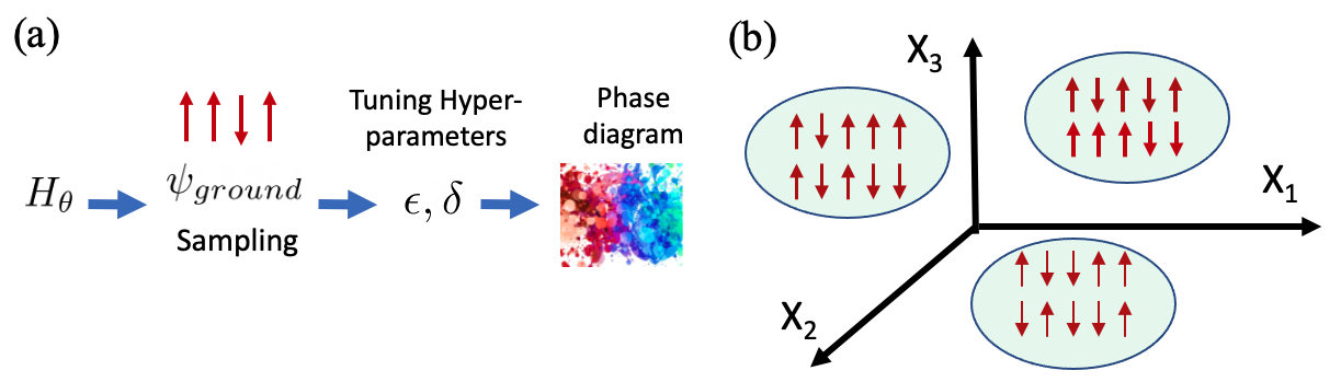
Let us now apply the DMA explained above to our quantum many-body problem. We imagine we are given a Hamiltonian with a set of unknown parameters We assume that we have direct access to the ground state of a -particle many-body Hamiltonian and we can sample from its many-body wave function in the configuration space. In particular, in this study, for spin- chains our sampled wave function determines the configuration of the spins in the real space, and therefore, the components of the ’th input vector are . For our fermionic and hard-core bosonic Hamiltonians, the measured wave function is represented in the Fock space, and therefore, . In this setting, the schematic flowchart of our classification approach is illustrated in Fig.1, where denotes the ground state wave functions. In general, this state is a superposition of different product states. In the next step, the sampling is performed in the space of these product states resulting in the vectors by which we can produce the corresponding Laplacian matrix . Since, across quantum phase transitions usually a change in the relevant degrees of freedom that describe the system occurs, we expect that for a given accuracy , once the scale is chosen properly, the number of clusters obtained from should reveal the underlying phase diagram of the system.
To determine the proper regime for as the parameter that describes the dynamics of the diffusion process Coifman and Lafon (2006), we use the approximate analysis of the spectrum of proposed in Rodriguez-Nieva and Scheurer (2019); Lidiak and Gong (2020). Assuming clusters of samples with particles in different configuration states, the diffusion matrix will acquire a block-diagonal form with each block corresponding to a single such clusters. In this representation, diagonal elements are close to the identity while off-diagonal components are bounded by . Denoting the number of such clusters with , after diagonalizing , we will approximately have eigenvalues larger than and therefore the accuracy can be approximated by . Thus by choosing , we can find the number of clusters of a particular size . Consequently, since the number of particles in the clusters can change between to , we need to span the corresponding range of , to obtain the best value of empirically where changes in show a conspicuous change for different values of . Therefore, sharp changes in as a function of can be presumed to trace the topological phase transitions.
In what follows we employ the procedure above, and consider some of the most well-known models which describe SPT phases and we demonstrate that we can reproduce their phase diagram with an acceptable precision. We summarize our models in table 1 where for all models we have ) and we use periodic boundary conditions.
Model 1: Nontrivial SPT/Symmetry-protected trivial.— In this section, we ask whether we can distinguish between ground states with a trivial phase and a non trivial SPT phase (de Léséleuc et al., 2018). As one of the simplest models, we start with the interacting version of the SSH model which has been recently realized via Rydberg atoms and describes a topological phase transition between a SPT non-trivial and trivial phase. This model can be described by hard-core bosons . We consider two alternating coupling constants denoted by and between adjacent sites , where the former couples sites with odd , and the latter couples sites with even ,
| (3) |
As shown in de Léséleuc et al. (2018) this model is mapped to the fermionic SHH model whose energy spectrum consists of two bands separated by a spectral gap . Most importantly, this model for is a topologically trivial phase while for it becomes a topological SPT phase which with open boundary conditions hosts delocalized zero-energy edge modes. In this case, the symmetry group based on group cohomology classification only has one non-trivial topological phase since Using Jordan-Wigner transformation, the original representation of this model transforms into a spin chain Hamiltonian de Léséleuc et al. (2018):
| (4) |
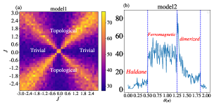
We use the natural spin basis as our sampling result. We can see in Fig. 2(a) that our method reproduces the phase diagram obtained in de Léséleuc et al. (2018).
Model 2: .— Here, compared to model 1, as a more challenging situation, we ask whether our approach can detect SPT phases with more involved symmetries where symmetry broken phases may exist, too. The Haldane phase of antiferromagnetic spin chains is a well-known example of such SPT phases with a symmetry group whose parent Hamiltonian can host several symmetry broken phases. An example of states in the Haldane phase which can be written in a closed form, is the AKLT state Affleck et al. (2004). This state is a special case of the ground state of the following bilinear-biquadratic spin- Hamiltonian ( are spin-1 operators) when ,
| (5) |
However, by varying this model describes two topological and non-topological phase transitions.
We can apply the DMA to this model with and plot the resulting phase diagram Fig. 2(b) which is akin to the results in Gils et al. (2013). Here, we again see another successful detection of an SPT phase where two additional symmetry broken phases may compete with each other.
Model 3: Variants of .— As an another more complicated model, we study a variant of the model where in addition to symmetry borken and topological phases we also have a time reversal invariant (TRI) phase with the same symmetries as the Haldane phase Gu and Wen (2009),
| (6) |
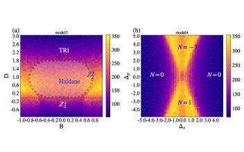
This Hamiltonian is invariant under translational symmetry, time reversal symmetry and parity symmetry. The complete description of the phase diagram is found in Gu and Wen (2009) which contains a time reversal invariant (TRI) phase with , and two symmetry broken phases, , and the Haldane phase. Our results for this model is depicted in Fig. 3(a). In this figure by comparing our phase diagram with those obtained in Gu and Wen (2009), we can see a noticeable transition between the , TRI and the Haldane phase. However, the distinction between the and the Haldane phase is less pronounced and we only see a partial change of color between these two regions.
Model 4.— In models based on group cohomology arguments the topological classification of the phases is described by the group, and there is only one topologically non-trivial phase. Here, in addition to spin- chains, we consider a weakly interacting fermionic spin- Hamiltonian which can host more than one non-trivial SPT phase whose topological classification is described by the group. This model respects both time reversal symmetry and spin-rotation symmetries. Hence, in the absence of interactions, based on the -fold classification, its topological phases are described by the group. Nevertheless, by adding interactions to this Hamiltonian, the resulting topological classes of this system will reduce to the group. The BdG form of this Hamiltonian is given by, (Tang and Wen, 2012):
| (7) |
where the last term is an unconventional pairing between electrons on adjacent sites. This model, can host three phases labeled by , which represents the states with distinct zero modes 111As demonstrated in Tang and Wen (2012) by stacking two chains with , we get another non-trivial phase with two zero modes. In the presence of strong interactions the phase with and are identified and hence the classification is .. We simulate this model with , and plot the resulting phase diagram in Fig. 3(b).
As we can in this figure, our approach can regenerate the phase diagram of this model as obtained in Tang and Wen (2012) with a high accuracy. To be more specific, we see sharp transitions between the topologically non-trivial phases with and trivial phases labeled by . While in principle, from this plot we cannot distinguish the phases from each other, from the fact that we see a conspicuous change in the number of eigenvalues at their intersection at we may speculate that the two regions correspond to distinct phases. This indicates that DMA not only can differentiate between topologically trivial phases and topologically non-trivial phases, but also can provide evidence for differentiating between different topological phases with similar properties.
Discussion and Outlook.—
In this work, we have used an unsupervised learning algorithm called diffusion maps to detect topological phase transitions between different symmetry broken phases and different SPT phases. Our results demonstrate that using diffusion maps as a computationally inexpensive method, can provide helpful evidence for the presence of SPT phase transitions and SPT phases. Since previously this algorithm has been used for detecting other symmetry broken phase transitions in one dimension Lidiak and Gong (2020), and due to the lack of intrinsic topological order in one dimension, our results demonstrate that the DMA can detect all different types of equilibrium phase transitions in one dimension.
From a conceptual viewpoint, the reason behind the efficacy of the DMA in detecting SPT phases is thought-provoking. One possible explanation is that the DMA in the continuum limit approximates the differential heat equation. On the other hand, the spectrum of elliptic differential operators such as the heat kernel appearing in the heat equation, can include important information about topological invariants Atiyah et al. (1975a, b). Based on our results, we speculate that these conceptual relations between the spectrum of differential operators and SPT invariants have practical application for computational and experimental purposes.
An immediate question to be pursued in future is the detection of SPT phases in higher dimensions via the DMA. Another intriguing question to investigate, is the detection of long-range topological order in symmetry enriched topological phases Mesaros and Ran (2013) which can be realized in two and higher dimensions without using thermal sampling Scheurer and Slager (2020). Also, detection of topological phases in non-equilibrium phases of matter especially Floquet systems is left for future studies.
Acknowledgements.
We are grateful to useful discussions with Mohammad Hafezi, Victor Albert, and Alireza Seif for helpful discussions. We acknowledge funding from MURI-AFOSR FA95501610323 and MURI-ARO W911NF-15-1-0397.References
- Wen (2017) Xiao-Gang Wen, “Colloquium: Zoo of quantum-topological phases of matter,” Reviews of Modern Physics 89, 041004 (2017).
- Wen and Niu (1990) Xiao-Gang Wen and Qian Niu, “Ground-state degeneracy of the fractional quantum hall states in the presence of a random potential and on high-genus riemann surfaces,” Physical Review B 41, 9377 (1990).
- Kane and Mele (2005) C. L. Kane and E. J. Mele, “ topological order and the quantum spin hall effect,” Phys. Rev. Lett. 95, 146802 (2005).
- Bernevig et al. (2006) B. Andrei Bernevig, Taylor L. Hughes, and Shou-Cheng Zhang, “Quantum spin hall effect and topological phase transition in hgte quantum wells,” Science 314, 1757–1761 (2006).
- Moore and Balents (2007) J. E. Moore and L. Balents, “Topological invariants of time-reversal-invariant band structures,” Phys. Rev. B 75, 121306 (2007).
- Fu et al. (2007) Liang Fu, C. L. Kane, and E. J. Mele, “Topological insulators in three dimensions,” Phys. Rev. Lett. 98, 106803 (2007).
- König et al. (2007) Markus König, Steffen Wiedmann, Christoph Brüne, Andreas Roth, Hartmut Buhmann, Laurens W. Molenkamp, Xiao-Liang Qi, and Shou-Cheng Zhang, “Quantum spin hall insulator state in hgte quantum wells,” Science 318, 766–770 (2007), https://science.sciencemag.org/content/318/5851/766.full.pdf .
- Hsi (2008) “A topological dirac insulator in a quantum spin hall phase,” Nature 452, 970–974 (2008).
- Hasan and Moore (2011) M. Zahid Hasan and Joel E. Moore, “Three-dimensional topological insulators,” Annual Review of Condensed Matter Physics 2, 55–78 (2011), https://doi.org/10.1146/annurev-conmatphys-062910-140432 .
- Altland and Zirnbauer (1997) Alexander Altland and Martin R. Zirnbauer, “Nonstandard symmetry classes in mesoscopic normal-superconducting hybrid structures,” Phys. Rev. B 55, 1142–1161 (1997).
- Schnyder et al. (2008) Andreas P. Schnyder, Shinsei Ryu, Akira Furusaki, and Andreas W. W. Ludwig, “Classification of topological insulators and superconductors in three spatial dimensions,” Phys. Rev. B 78, 195125 (2008).
- Kitaev (2009) Alexei Kitaev, “Periodic table for topological insulators and superconductors,” in AIP conference proceedings, Vol. 1134 (American Institute of Physics, 2009) pp. 22–30.
- Chen et al. (2012) Xie Chen, Zheng-Cheng Gu, Zheng-Xin Liu, and Xiao-Gang Wen, “Symmetry-protected topological orders in interacting bosonic systems,” Science 338, 1604–1606 (2012).
- Barkeshli et al. (2019) Maissam Barkeshli, Parsa Bonderson, Meng Cheng, and Zhenghan Wang, “Symmetry fractionalization, defects, and gauging of topological phases,” Phys. Rev. B 100, 115147 (2019).
- Pollmann and Turner (2012) Frank Pollmann and Ari M. Turner, “Detection of symmetry-protected topological phases in one dimension,” Phys. Rev. B 86, 125441 (2012).
- Haegeman et al. (2012) Jutho Haegeman, David Pérez-García, Ignacio Cirac, and Norbert Schuch, “Order parameter for symmetry-protected phases in one dimension,” Phys. Rev. Lett. 109, 050402 (2012).
- Shiozaki and Ryu (2017) Ken Shiozaki and Shinsei Ryu, “Matrix product states and equivariant topological field theories for bosonic symmetry-protected topological phases in (1+1) dimensions,” Journal of High Energy Physics 2017, 100 (2017).
- Dehghani et al. (2021) Hossein Dehghani, Ze-Pei Cian, Mohammad Hafezi, and Maissam Barkeshli, “Extraction of the many-body chern number from a single wave function,” Phys. Rev. B 103, 075102 (2021).
- Elben et al. (2020) Andreas Elben, Jinlong Yu, Guanyu Zhu, Mohammad Hafezi, Frank Pollmann, Peter Zoller, and Benoît Vermersch, “Many-body topological invariants from randomized measurements in synthetic quantum matter,” Science Advances 6 (2020), 10.1126/sciadv.aaz3666, https://advances.sciencemag.org/content/6/15/eaaz3666.full.pdf .
- Cian et al. (2021) Ze-Pei Cian, Hossein Dehghani, Andreas Elben, Benoît Vermersch, Guanyu Zhu, Maissam Barkeshli, Peter Zoller, and Mohammad Hafezi, “Many-body chern number from statistical correlations of randomized measurements,” Phys. Rev. Lett. 126, 050501 (2021).
- Carrasquilla and Melko (2017) Juan Carrasquilla and Roger G Melko, “Machine learning phases of matter,” Nature Physics 13, 431 (2017).
- Wetzel (2017) Sebastian J Wetzel, “Unsupervised learning of phase transitions: From principal component analysis to variational autoencoders,” Physical Review E 96, 022140 (2017).
- Van Nieuwenburg et al. (2017) Evert PL Van Nieuwenburg, Ye-Hua Liu, and Sebastian D Huber, “Learning phase transitions by confusion,” Nature Physics 13, 435 (2017).
- Kuo et al. (2021) En-Jui Kuo, Alireza Seif, Rex Lundgren, Seth Whitsitt, and Mohammad Hafezi, “Decoding conformal field theories: from supervised to unsupervised learning,” arXiv preprint arXiv:2106.13485 (2021).
- van Nieuwenburg et al. (2018) Evert van Nieuwenburg, Eyal Bairey, and Gil Refael, “Learning phase transitions from dynamics,” Physical Review B 98, 060301 (2018).
- Schindler et al. (2017) Frank Schindler, Nicolas Regnault, and Titus Neupert, “Probing many-body localization with neural networks,” Physical Review B 95, 245134 (2017).
- Seif et al. (2021) Alireza Seif, Mohammad Hafezi, and Christopher Jarzynski, “Machine learning the thermodynamic arrow of time,” Nature Physics 17, 105–113 (2021).
- Carleo and Troyer (2017) Giuseppe Carleo and Matthias Troyer, “Solving the quantum many-body problem with artificial neural networks,” Science 355, 602–606 (2017).
- Torlai et al. (2018) Giacomo Torlai, Guglielmo Mazzola, Juan Carrasquilla, Matthias Troyer, Roger Melko, and Giuseppe Carleo, “Neural-network quantum state tomography,” Nature Physics 14, 447 (2018).
- Carrasquilla et al. (2019) Juan Carrasquilla, Giacomo Torlai, Roger G Melko, and Leandro Aolita, “Reconstructing quantum states with generative models,” Nature Machine Intelligence 1, 155 (2019).
- Seif et al. (2018) Alireza Seif, Kevin A Landsman, Norbert M Linke, Caroline Figgatt, C Monroe, and Mohammad Hafezi, “Machine learning assisted readout of trapped-ion qubits,” Journal of Physics B: Atomic, Molecular and Optical Physics 51, 174006 (2018).
- Torlai et al. (2019) Giacomo Torlai, Brian Timar, Evert PL van Nieuwenburg, Harry Levine, Ahmed Omran, Alexander Keesling, Hannes Bernien, Markus Greiner, Vladan Vuletić, Mikhail D Lukin, et al., “Integrating neural networks with a quantum simulator for state reconstruction,” arXiv preprint arXiv:1904.08441 (2019).
- Deng et al. (2017) Dong-Ling Deng, Xiaopeng Li, and S. Das Sarma, “Machine learning topological states,” Phys. Rev. B 96, 195145 (2017).
- Venderley et al. (2018) Jordan Venderley, Vedika Khemani, and Eun-Ah Kim, “Machine learning out-of-equilibrium phases of matter,” Phys. Rev. Lett. 120, 257204 (2018).
- Zhang et al. (2018) Pengfei Zhang, Huitao Shen, and Hui Zhai, “Machine learning topological invariants with neural networks,” Phys. Rev. Lett. 120, 066401 (2018).
- Ni et al. (2019) Qi Ni, Ming Tang, Ying Liu, and Ying-Cheng Lai, “Machine learning dynamical phase transitions in complex networks,” Phys. Rev. E 100, 052312 (2019).
- Huang et al. (2021) Hsin-Yuan Huang, Richard Kueng, and John Preskill, “Information-theoretic bounds on quantum advantage in machine learning,” Phys. Rev. Lett. 126, 190505 (2021).
- Wang (2016) Lei Wang, “Discovering phase transitions with unsupervised learning,” Phys. Rev. B 94, 195105 (2016).
- Hu et al. (2017) Wenjian Hu, Rajiv R. P. Singh, and Richard T. Scalettar, “Discovering phases, phase transitions, and crossovers through unsupervised machine learning: A critical examination,” Phys. Rev. E 95, 062122 (2017).
- Coifman et al. (2005) Ronald R Coifman, Stephane Lafon, Ann B Lee, Mauro Maggioni, Boaz Nadler, Frederick Warner, and Steven W Zucker, “Geometric diffusions as a tool for harmonic analysis and structure definition of data: Diffusion maps,” Proceedings of the national academy of sciences 102, 7426–7431 (2005).
- Lidiak and Gong (2020) Alexander Lidiak and Zhexuan Gong, “Unsupervised machine learning of quantum phase transitions using diffusion maps,” arXiv preprint arXiv:2003.07399 (2020).
- Rodriguez-Nieva and Scheurer (2019) Joaquin F Rodriguez-Nieva and Mathias S Scheurer, “Identifying topological order through unsupervised machine learning,” Nature Physics 15, 790–795 (2019).
- Scheurer and Slager (2020) Mathias S Scheurer and Robert-Jan Slager, “Unsupervised machine learning and band topology,” Physical Review Letters 124, 226401 (2020).
- den Nijs and Rommelse (1989) Marcel den Nijs and Koos Rommelse, “Preroughening transitions in crystal surfaces and valence-bond phases in quantum spin chains,” Phys. Rev. B 40, 4709–4734 (1989).
- Oshikawa (1992) M Oshikawa, “Hidden symmetry in quantum spin chains with arbitrary integer spin,” Journal of Physics: Condensed Matter 4, 7469–7488 (1992).
- Kennedy and Tasaki (1992a) Tom Kennedy and Hal Tasaki, “Hidden × symmetry breaking in haldane-gap antiferromagnets,” Phys. Rev. B 45, 304–307 (1992a).
- Levin and Wen (2006) Michael Levin and Xiao-Gang Wen, “Detecting topological order in a ground state wave function,” Phys. Rev. Lett. 96, 110405 (2006).
- Kitaev and Preskill (2006) Alexei Kitaev and John Preskill, “Topological entanglement entropy,” Phys. Rev. Lett. 96, 110404 (2006).
- Li and Haldane (2008) Hui Li and F. D. M. Haldane, “Entanglement spectrum as a generalization of entanglement entropy: Identification of topological order in non-abelian fractional quantum hall effect states,” Phys. Rev. Lett. 101, 010504 (2008).
- Calabrese and Lefevre (2008) Pasquale Calabrese and Alexandre Lefevre, “Entanglement spectrum in one-dimensional systems,” Phys. Rev. A 78, 032329 (2008).
- de Léséleuc et al. (2018) Sylvain de Léséleuc, Vincent Lienhard, Pascal Scholl, Daniel Barredo, Sebastian Weber, Nicolai Lang, Hans Peter Büchler, Thierry Lahaye, and Antoine Browaeys, “Experimental realization of a symmetry protected topological phase of interacting bosons with rydberg atoms,” arXiv preprint arXiv:1810.13286 (2018).
- Preskill (2018) John Preskill, “Quantum computing in the nisq era and beyond,” Quantum 2, 79 (2018).
- De la Porte et al. (2008) J De la Porte, BM Herbst, W Hereman, and SJ Van Der Walt, “An introduction to diffusion maps,” in Proceedings of the 19th Symposium of the Pattern Recognition Association of South Africa (PRASA 2008), Cape Town, South Africa (2008) pp. 15–25.
- Jolliffe and Cadima (2016) Ian T Jolliffe and Jorge Cadima, “Principal component analysis: a review and recent developments,” Philosophical Transactions of the Royal Society A: Mathematical, Physical and Engineering Sciences 374, 20150202 (2016).
- (55) see Supplemental Material .
- Coifman and Lafon (2006) Ronald R Coifman and Stéphane Lafon, “Diffusion maps,” Applied and computational harmonic analysis 21, 5–30 (2006).
- Affleck et al. (2004) Ian Affleck, Tom Kennedy, Elliott H Lieb, and Hal Tasaki, “Rigorous results on valence-bond ground states in antiferromagnets,” in Condensed Matter Physics and Exactly Soluble Models (Springer, 2004) pp. 249–252.
- Gils et al. (2013) Charlotte Gils, Eddy Ardonne, Simon Trebst, David A Huse, Andreas WW Ludwig, Matthias Troyer, and Zhenghan Wang, “Anyonic quantum spin chains: Spin-1 generalizations and topological stability,” Physical Review B 87, 235120 (2013).
- Gu and Wen (2009) Zheng-Cheng Gu and Xiao-Gang Wen, “Tensor-entanglement-filtering renormalization approach and symmetry-protected topological order,” Physical Review B 80, 155131 (2009).
- Tang and Wen (2012) Evelyn Tang and Xiao-Gang Wen, “Interacting one-dimensional fermionic symmetry-protected topological phases,” Phys. Rev. Lett. 109, 096403 (2012).
- Note (1) As demonstrated in Tang and Wen (2012) by stacking two chains with , we get another non-trivial phase with two zero modes. In the presence of strong interactions the phase with and are identified and hence the classification is .
- Atiyah et al. (1975a) M. F. Atiyah, V. K. Patodi, and I. M. Singer, “Spectral asymmetry and riemannian geometry. i,” Mathematical Proceedings of the Cambridge Philosophical Society 77, 43–69 (1975a).
- Atiyah et al. (1975b) M. F. Atiyah, V. K. Patodi, and I. M. Singer, “Spectral asymmetry and riemannian geometry. ii,” Mathematical Proceedings of the Cambridge Philosophical Society 78, 405–432 (1975b).
- Mesaros and Ran (2013) Andrej Mesaros and Ying Ran, “Classification of symmetry enriched topological phases with exactly solvable models,” Phys. Rev. B 87, 155115 (2013).
- Kennedy and Tasaki (1992b) Tom Kennedy and Hal Tasaki, “Hidden symmetry breaking and the haldane phase in s= 1 quantum spin chains,” Communications in mathematical physics 147, 431–484 (1992b).
SUPPLEMENTAL MATERIAL
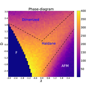
In this supplemental, we consider two additional spin chain models which can host SPT phases. We consider the following Hamiltonian with periodic boundary condition as considered for other models in the main text, (Kennedy and Tasaki, 1992b):
| (8) |
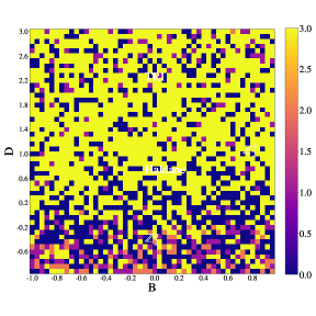
We can use the same techniques and with and samples to implement the diffusion map algorithm (DMA). We plot the phase diagram via the DMA. The phase diagram Fig. 4 matches with the predictions in (Kennedy and Tasaki, 1992b) to a great extent. In particular the distinction between the antiferromagnetic phase (AFM), Haldane and the ferromagnetic phases are completely distinguishable, however, we observe a less evident transition between the Haldane and the dimerized phases. We also notice that we have not detected the phase whose presence is still undetermined via exact methods (Kennedy and Tasaki, 1992b).
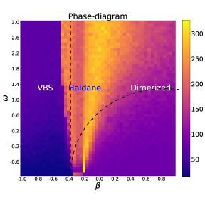
The second model that we consider here is the following spin Hamiltonian with periodic boundary condition (Kennedy and Tasaki, 1992b):
| (9) |
for even, for is odd. We can see our method Fig. 5 matches qualitatively with (Kennedy and Tasaki, 1992b) and we can see a sharp transition between the topological Haldane phase and two symmetry broken phases i.e. valence bond state (VBS) and dimerized phases. We can also predict (Kennedy and Tasaki, 1992b) for the transition from VBS to Haldane phase.
III PCA and k-means algorithm
To compare the performance of the diffusion maps algorithm and other unsupervised methods, here, we try one of the most standard unsupervised algorithm called PCA (principle component analysis) on our sampling and compute the mean of components. After doing this, we choose the number of clusters and use the standard means algorithm. It should be highlighted that we do not have to pick the number of clusters in the diffusion map algorithm. We choose model 3 Gu and Wen (2009) in our main text.
| (10) |
Here, we find that this method fails to identify the phase transition in fig 6 completely. This superior performance of the diffusion maps in comparison to other unsupervised learning methods, is due to the fact that in this approach we use non-linear kernel functions which allow us to detect complicated non-linear structures in data sets.