Ocean Mover’s Distance: Using Optimal Transport for Analyzing Oceanographic Data

Abstract

Remote sensing observations from satellites and global biogeochemical models have combined to revolutionize the study of ocean biogeochemical cycling, but comparing the two data streams to each other and across time remains challenging due to the strong spatial-temporal structuring of the ocean. Here, we show that the Wasserstein distance provides a powerful metric for harnessing these structured datasets for better marine ecosystem and climate predictions. Wasserstein distance complements commonly used point-wise difference methods such as the root mean squared error, by quantifying differences in terms of spatial displacement in addition to magnitude. As a test case we consider Chlorophyll (a key indicator of phytoplankton biomass) in the North-East Pacific Ocean, obtained from model simulations, in situ measurements, and satellite observations. We focus on two main applications: 1) Comparing model predictions with satellite observations, and 2) temporal evolution of Chlorophyll both seasonally and over longer time frames. Wasserstein distance successfully isolates temporal and depth variability and quantifies shifts in biogeochemical province boundaries. It also exposes relevant temporal trends in satellite Chlorophyll consistent with climate change predictions. Our study shows that optimal transport vectors underlying Wasserstein distance provide a novel visualization tool for testing models and better understanding temporal dynamics in the ocean.

Subjects: Climatology, Oceanography

Keywords: Wasserstein distance, Earth mover’s distance, Data-model comparison, Optimal Transport, Chlorophyll, Remote Sensing

1. Introduction

Understanding the differences between large spatiotemporal datasets is a common task in oceanography. Whether quantifying the agreement between the output of an ocean simulation model Dutkiewicz et al. (2015); Forget et al. (2015a) and in situ measurement Moore et al. (2009); Jackson et al. (2017) or monitoring the changes in the ocean across time Dutkiewicz et al. (2019), one needs a meaningful notion of “distance” between scalar fields defined across the ocean. We focus on the case in which the scalar field of interest represents the density or concentration of a quantity over space. It is most common to compare images or data distributions using a “pixel-by-pixel” or pointwise difference Seegers et al. (2018); Forget et al. (2015a); Forget and Ponte (2015); Forget et al. (2015b); popular examples of such distances include root-mean-squared error (RMSE) and mean absolute error. However, although easy to compute, pixel-wise comparisons may not fully account for the spatiotemporal nature of ocean data, which can exhibit complicated patterns composed of both global and local underlying trends linked to shifting and evolving water mass bodies.

These issues are well known and have led to the development of various normalized differences or “cost functions” which differentially weight differences arising from deviations in quantity, location or from unresolved scales (e.g. Forget and Wunsch (2007); Forget et al. (2015a); Forget and Ponte (2015)). Focusing on the probability distribution over predefined regions (e.g., marine provinces, or water masses) is one way to account for spatial errors. This method has been used to examine, for example: the volumetric census of water masses Forget (2010); Speer and Forget (2013); relationships between primary production and export Cael et al. (2018); and the effects of mesoscale eddies Ashkezari et al. (2016). Power-spectra further provide a useful basis for comparison as a function of space and/or time scale (e.g. Forget and Ponte (2015), McCaffrey et al. (2015)). Despite these advances there remains a need for metrics which take into account pattern differences in a clear and interpretable way. This is especially true when evaluating the skill (or error) of ocean biogeochemical model simulations compared to other data sources such as satellite-derived measurements. Indeed, a recent summary paper ioc (2020) reports the need for a better measure of ocean Chlorophyll difference that goes beyond pixel-wise differences. The reasons are many. Computer simulations may not be finely resolved enough to capture meso-scale Chlorophyll patterns (e.g. eddies) in time and space. However, such features will be captured in situ and using satellites. Further, small spatial mismatches can result in large pixel-wise differences – see Section 5.3.2 of ioc (2020) – which penalize models that are mechanistically correct for stochastic fluctuations. What we need is a metric which is easy to interpret, like RMSE, but for pattern differences.

In this paper, we explore the use of the Wasserstein distance Villani (2021), which sometimes goes by the name earth mover’s distance Rubner et al. (2000). As that name suggests, Wasserstein distance measures the total amount of ”dirt”-moving that would be required to transform one mound of dirt (representing a probability distribution) to make it equivalent to another mound (a second probability distribution). The probability distributions in our context are normalized versions of the scalar fields. Unlike pixel-by-pixel distances, the Wasserstein distance incorporates the spatial structure of discrepancies, making it particularly well-suited for the comparison of ocean datasets. Wasserstein distance has been used in several other areas of geosciences. To list a few, it has been used to analyze particle distributions in the ocean Nooteboom et al. (2020), for measuring error in temperature, precipitation, and sea ice projections Vissio et al. (2020), for ocean data assimilation Tamang et al. (2020); Le et al. (2021), for analyzing sea height imagesPapadakis (2015), for ocean Synthetic Aperture Radar (SAR) segmentation Colin et al. (2021), and for studying sea ice imagery Parno et al. (2019). However, ioc (2020) makes clear that Wasserstein distance has not been thoroughly applied to the fundamental problem of model-to-data comparison and model-skill evaluation particularly in the context of ocean biogeochemical models and the representation of marine ecosystem structure and function. The goal of this paper is to carefully highlight the usefulness of Wasserstein distance in this context, as well as to show its usefulness in exploring time series of satellite maps. We focus on high-coverage Chlorophyll observations in the North Pacific Subtropical Gyre Jackson et al. (2017), and demonstrate how discrepancies between model predictions and observed Chlorophyll can be interpreted in terms of a transport field that when integrated over space yields a measure of distance in spatial units. We do this for the comparison of surface maps (see Section 3(a)) and of depth profiles (see Section 3(b)), which reveals long-term temporal trend and seasonality of satellite and model Chlorophyll maps in Section 3(a)(ii).

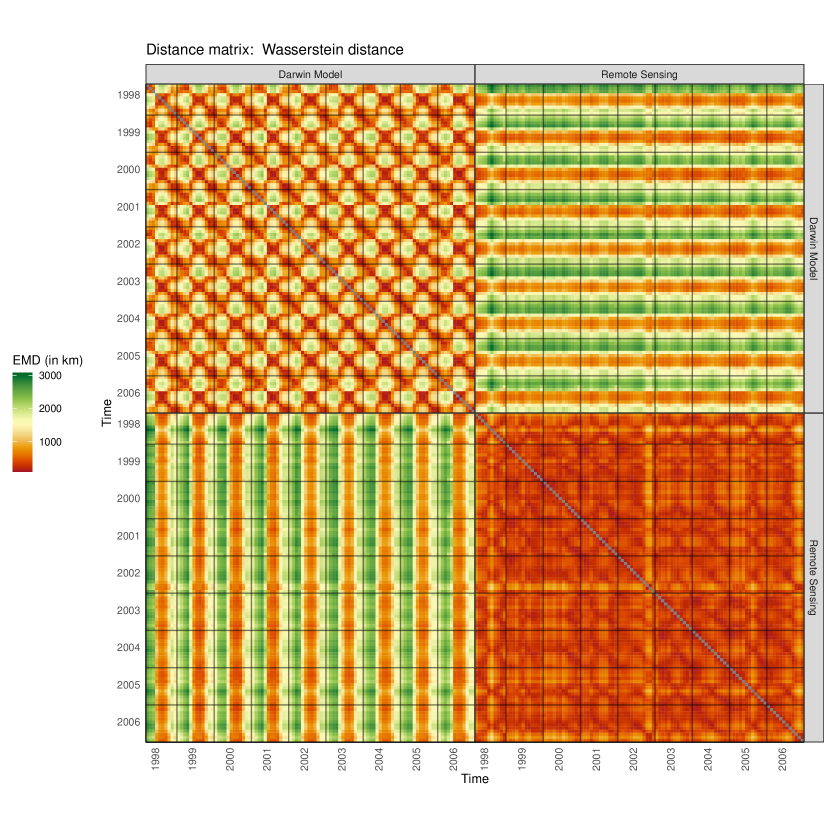
Figure 1: All pairwise Wasserstein distances from all monthly maps between 1998 and 2006, from the two data sources (Darwin and remote-sensing), as a $24\times 24$ distance matrix. Figure S4 shows a classical MDS performed on this data.

To convey the intuitive appeal of the Wasserstein distance over pixel-wise distance measures, consider the toy example in Figure 1, in which we imagine two surface maps that are identical except for the location of an artificially inserted patch of Chlorophyll south of the Equator. Physical processes like, for example, Rossby waves can generate such propagating patches. The right panel shows how RMSE and Wasserstein distance quantify the difference between the two surface maps as spatial shift of the patch increases. RMSE quickly saturates: once the two patches have no spatial overlap, there is no further change in the RMSE metric. By contrast, the Wasserstein distance increases in an approximately linear fashion. Indeed, the Wasserstein distance has units of distance and is directly related to the distance that the patch has moved.

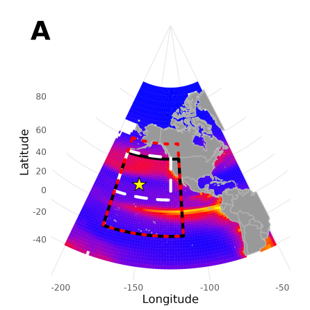
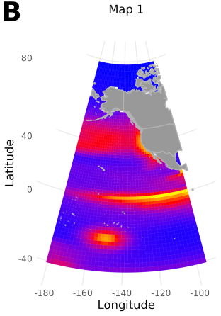
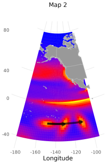
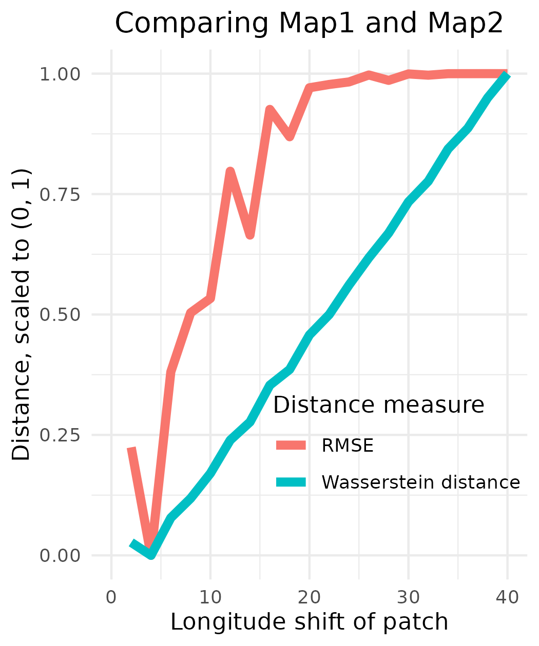
Figure 1: The left-most panel A shows a map of the study regions that are used for data analysis in this paper (solid lines for Section 3(a)(i), dotted lines for 3(a)(ii), and dashed lines for Section 3(a)(iii)); the star marker denotes the location of station ALOHA near Hawaii from which we obtain depth profiles of Chlorophyll to analyze in Section 3(b). In panel B, the first two figures show a toy example of two Chlorophyll maps both formed using simulated climatology data in January (from the ocean coupled physical-biogeochemical-optical model Dutkiewicz et al. (2015); Forget et al. (2015a)). One map was formed by adding an artificial patch of Chlorophyll to a longitude of –150. The other map was formed by shifting this patch to the east by up to 40 degrees longitude (while also rotating it). The right-most graph shows two different distance measures—root-mean-squared error (RMSE) and Wasserstein distance—between the two plots, while varying the amount of longitude shift of the patch. RSME plateaus after a shift of 20 degrees, while the Wasserstein distance is proportional to the amount of shift.

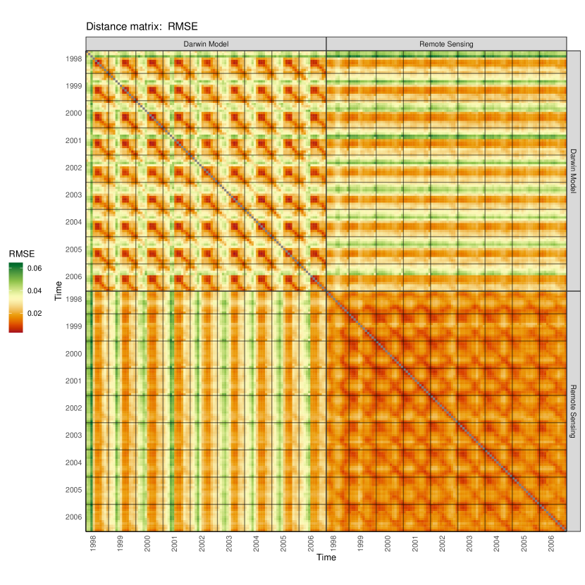
Figure 2: Showing RMSE distance matrix (analogous to Figure S1).

In addition to its merit as a scalar distance, the Wasserstein distance also enables the visualization of the transport that would most efficiently (from the perspective of a person moving the dirt) transform the first ocean map into the second. For example, the rightmost panel of Figure 2A shows the optimal transport pattern between the two maps on the left (see Section 3(a)(i)). These optimal transport patterns are not to be interpreted as “physical” transport of the underlying quantity. Still, these optimal transport patterns are useful for understanding how the data differ. In this work, we consider two primary types of comparison: (1) comparing two different data sources measuring the same signal on a spatiotemporal region or gridpoints; and (2) comparing the same data source at different times. In both cases, visualizing the optimal transport can provide a scenario to elucidate the nature of the difference. This can be particularly useful when spatiotemporal differences are related to shifts in patterns that may not be well captured by pixel-wise comparisons.

With this paper, we aim to highlight the usefulness of studying ocean data using Wasserstein distance, which we show is particularly well-suited for evaluation of ocean biogeochemical models, among many other applications. We compare satellite Chlorophyll observations from the Eastern North Pacific Ocean and depth profiles from the North Pacific Subtropical Gyre (NPSG) with their counterparts from a biogeochemical model coupled to a state estimate of the ocean currents, temperature, and salinity Forget et al. (2015a). We show that the Wasserstein distance for Chlorophyll between model and satellite data is large compared to the Wasserstein distance over the seasonal cycle from satellite data or the model. We further show how Wasserstein distance can be used to track changes in the transitional boundaries between marine provinces over time Follett et al. (2021). When reduced to this “feature comparison” we find that the model and satellite observations are in relatively close agreement. Furthermore, applying a similar analysis to the Chlorophyll depth profiles at Station ALOHA Karl and Lukas (1996); Karl and Church (2014), discrepancy between model outputs and in situ data is framed in terms of Chlorophyll shifts along the depth dimension. Our numerical experiments allowed us to investigate whether the Wasserstein distance can effectively capture deviations in the “Deep Chlorophyll Maximum” between two Chlorophyll depth profiles Venrick et al. (1973); Cullen (1982); Huisman et al. (2006). These results provide a path and justification for using Wasserstein distance to analyze deviations in terms of pattern displacements, and provide complementary information on magnitude differences.

2. Material and Methods

(a) Wasserstein Distance

Consider two discrete probability distributions $P=(P_{i})_{i=1}^{m},Q=(Q_{j})_{j=1}^{n},$ such that $P_{i}\geq 0$ for all $i$, $Q_{j}\geq 0$ for all $j$, and $\sum_{i}P_{i}=\sum_{j}Q_{j}=1$. In our context, $i=1,\ldots,m$ indexes a spatial partition of the region of ocean being studied into $m$ cells (and likewise for $j=1,\ldots,n$) and $P_{i}$ gives the proportion of the Chlorophyll (or any other positive quantity the scalar field is representing) in the region that is in cell $i$. In the special case that $i$ and $j$ index the same set of cells (such as $m=n$ pixels), one can define pixel-wise distances such as the root-mean-squared error, $\mathrm{RMSE}(P,Q)=\left(\frac{1}{n}\sum_{i}(P_{i}-Q_{i})^{2}\right)^{1/2}$. If $P$ and $Q$ do not exist on the same coordinates, they need to be reconciled (processed) to exist on the exact same cells in order to calculate RMSE. This requirement is not shared by Wasserstein distance, which we describe next.

Wasserstein distance, which is also sometimes called earth mover’s distance Rubner et al. (2000), as discussed in the introduction can be thought of as the total amount of “dirt”-moving required to transform a mound shaped like $P$ to a mound shaped like $Q$ when one performs optimal transport Monge (1781); Kantorovitch (1958); Villani (2021), i.e. when one does this earth moving in the most efficient fashion possible. More precisely, the optimal transport between $P$ and $Q$ can be expressed as solving the following linear program:

$$\hat{f}=\mathop{\mathrm{argmin}}_{f}{\sum_{i=1}^{m}\sum_{j=1}^{n}f_{i,j}d_{i,j}^{2}},\text{ subject to }\begin{cases}\forall i,j:f_{i,j}\geq 0\\ \forall i:\sum_{j}f_{i,j}=P_{i}\\ \forall j:\sum_{i}f_{i,j}=Q_{j},\\ \end{cases}$$ (1)

where $d_{i,j}$ is the base distance between cell $i$ in $P$ and cell $j$ in $Q$. The optimization variable $f_{i,j}$ describes the amount of probability mass being transported from $i$ to $j$. The constraints encode that no mass is created or destroyed and that the net effect of the transport is to take $P$ to $Q$. The objective function is a weighted sum of squared distances (the square used in this paper makes this the ”2-Wasserstein” distance), where the weights are given by the amount of probability mass being transported across all pairs of cells, $i$ and $j$. The optimum $\hat{f}$ is the optimal transport between $P$ and $Q$, and the Wasserstein distance is defined to be the square root of the optimal value of this optimization problem: $\mathrm{W_{2}}(P,Q)=\left(\sum_{i=1}^{m}\sum_{j=1}^{n}\hat{f}_{i,j}d_{i,j}^{2}\right)^{1/2}$.

Throughout, we use the transport R package Schuhmacher et al. (2020), which implements the algorithm in Bonneel et al. (2011) in which each discrete probability distribution first undergoes a multiscale transformation and is decomposed into a weighted sum of Gaussian bases; then the optimal transport problem is solved using a network simplex algorithm. This has $O(nm)$ computational complexity. Solving the optimal transport problem with a full dense $d_{i,j}$ (base distance matrix as in equation (1)) is prohibitively slow at moderate problem sizes like $n=m=10,000$. One interesting and straightforward future improvement is to reduce the number of transports needed by setting $d_{i,j}=\infty$ if $|i-j|>c$ for some threshold $c$. Generally, there is a large literature on algorithms to calculate optimal transport, of which we cite only a recent few. Among popular cutting-edge algorithms are fast approximations in the Fourier space Auricchio et al. (2020) and in the wavelet space Shirdhonkar and Jacobs (2008). Also popular is entropic regularization Cuturi (2013), which is known as Sinkhorn distance. The most analogous pre-existing application of Wasserstein distance is to digital image data, and has gained popularity in recent years in the neural network literature Rubner et al. (2000).

A distinctive feature of ocean applications (as opposed to, for example, digital image applications), is that the base distance $d_{i,j}$ cannot be taken to be Euclidean distance, especially when the coordinates of the cells $i$ and $j$ are far apart. Instead, we take the base distance to be the great circle distance between the (longitude, latitude) coordinates, which we compute using the geodist package in R Padgham and Sumner (2021). Our work also offers fully reproducible code, via an R package named omd (https://github.com/sangwon-hyun/omd), which could be used for other ocean studies.

(b) Multidimensional Scaling

In our analysis, multidimensional scaling plots will be used to help us interpret distance matrices, often highlighting seasonality and other relationships across time. Using Wasserstein distance as described in Section 2(a), we can take a collection of maps and form a distance matrix $D\in\mathbb{R}^{N\times N}$, where $D_{ab}$ is the Wasserstein distance between normalized Chlorophyll maps $a$ and $b$. To help interpret the resulting distance matrix, we visualize the maps’ relationship to each other using classical multidimensional scaling (classical MDS) Borg and Groenen (2005); Gower (1966). This popular data analysis technique seeks a configuration of points in the two-dimensional plane whose Euclidean distances are close to those in an inputted distance matrix. That is, after computing the Wasserstein distance between all pairs of $N$ maps, the goal is to find a low-dimensional embedding, $z_{1},\cdots,z_{N}\in\mathbb{R}^{2}$, for which $\|z_{a}-z_{b}\|_{2}\approx D_{ab}$ for all maps $1\leq a<b\leq N$. An approximate closed-form solution can be calculated using an eigen-decomposition of the doubly centered matrix of squared distances. The details are provided in Supplement Section S1(a).

(c) Data

The analysis is based on monthly Chlorophyll data from three different data sources: derived from ocean-color remote sensing observations, the output from a global biogeochemical circulation model, and integrated in situ observations. We use a subdomain of the model and remote sensing datasets focused on a latitude-longitude rectangle in the Pacific Ocean directly above—and including—Hawaii. The region is centered around about 20 degrees latitude and $-155$ degrees longitude and captures interesting geographic variability in the ocean. To the south of this region is the North Pacific Subtropical Gyre (low latitude, dominated by warm, more saline water) and to the north is the Subpolar Gyre (high latitude, low-temperature, low-salinity, nutrient-rich water). The region between these two gyres is the North-Pacific Transition Zone (NPTZ) with a strong gradient in Chlorophyll, as can be seen in the remote sensing observations and in the model output (Figure 2A, left panels). We also focus on data directly from a fixed location near the south of this region, Station ALOHA ($22.75$ degrees latitude and $-158$ degrees longitude) HOT (2021). Throughout, we exclude Chlorophyll data near the coastline where both satellite measurements and numerical models have known irregularities. Each dataset is described in some detail next.

(i) CBIOMES-global Model Output

Model data is based on output from a coupled physical-biogeochemical-optical model, modified for the Simons Collaboration on Computational Biogeochemical Modeling of Marine Ecosystems (CBIOMES) project. The CBIOMES-global model simulates the period from 1992-2011 Forget (2018).

The model’s physical component is derived from the Estimating the Circulation and Climate of the Ocean project (ECCO), version 4 (ECCOv4) Forget et al. (2015a, b); Forget and Ponte (2015). ECCOv4 uses a “least-squares with Lagrangian multipliers” method to get internal model parameters, initial, and boundary conditions that minimize the discrepancy between global observational data streams of satellite and in situ data. The end product is a global three-dimensional configuration state estimate, at a horizontal resolution of 1 degree and with depth ranging from 10 m at the surface to 500 m at depth (see Forget et al. (2015a) for details).

The biogeochemical/ecosystem component is from the MIT Darwin Project and follows that of Dutkiewicz et al. (2021). The model data we use in this paper is the aggregated Chlorophyll-a across all phytoplankton groups simulated from this ecosystem model, made into monthly averages. The amount of Chlorophyll in each of the $35$ phytoplankton types varies based on light, nutrients and temperature Geider et al. (1998). The $35$ phytoplankton types are from from several biogeochemical functional groups such as pico-phytoplankton, silicifying Diatoms, calcifying coccolithophores, mixotrophs that photosynthesize and graze, and nitrogen fixing diazotrophs, with sizes that span from 0.6 to 228 $\mu$m equivalent spherical diameter (ESD). The model incorporates various interactions with chemical factors (e.g. carbon, phosphorus, nitrogen, silica, iron, oxygen) and with other species (e.g. grazing by zooplankton). See Dutkiewicz et al. (2021) for full details. Hereon, we will simply refer to this data as model data.

(ii) Remote Sensing Data

Remote sensing (or satellite-derived) data is based on version 3.0 of the European Space Agency Ocean Colour Climate Change Initiative (OC-CCI) Mélin et al. (2017); Sathyendranath et al. (2019, 2020), a blended Level 4 Chlorophyll product with a spatial resolution of 4 km. The OC–CCI V5.0 combines data from five independent ocean-colour sensors to produce merged, climate-quality observations of Chlorophyll concentration. The sensors include the Sea-viewing Wide-Field-of-view Sensor (SeaWiFS), the Aqua MOderate-resolution Imaging Spectroradiometer (MODIS-Aqua), the MEdium spectralResolution Imaging Spectrometer (MERIS), the Suomo-NPP Visible InfraredImaging Radiometer Suite (NPP-VIIRS), and the Sentinel 3A Ocean and Land Colour Instrument (OLCI). These data sources are algorithmically merged and processed (see more details of this processing in Jackson et al. (2017); Sathyendranath et al. (2019)), then downscaled to the same spatial grid as model data at the monthly time resolution.

(iii) In-Situ Data from Station ALOHA

We additionally consider shipboard measured Chlorophyll-a from Station ALOHA (22°45’N, 158°00’W). The dataset (obtained from the Simons Collaborative Marine Atlas Project (CMAP), originally sourced from https://hahana.soest.hawaii.edu/hot/dataaccess.html) contains concentrations of Chlorophyll collected using a CTD fluorescence sensor. There are $28,583$ observations measured between 1988-10-3 to 2016-11-27, in the depth range between 0 and 200 meters. This data was downloaded directly from Hyun et al. (2019), an R package for accessing the CMAP database.

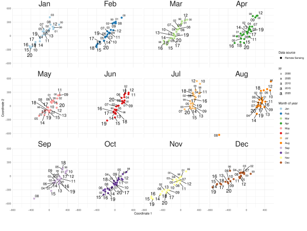
Figure 6: MDS of the interannualtime-resolved monthly remote sensing data in 1998-2020; this shows a long-term change of each calendar month. The labels show the last two digits of the four-digit year number. In many calendar months, the bottom-left of the points show later years (larger text). This shows additional evidence of a long-term change over time that was observed in Figure S5.

In Section 3(b), we compare depth profiles (measurements over depth) of in situ data and model data using Wasserstein distance. In situ data is sampled irregularly in time, while Darwin data is complete in space and time. In order to compile the two datasets at matching locations in space and time, we colocalize the model data, by taking averages of the Chlorophyll measurements in a certain space-time vicinity ($\pm 2$ days and $\pm 5$ meters) of each time point of the in situ data. Panel B of Figure 6 shows the Chlorophyll data from the two sources. Each depth profile is normalized by dividing by the total so that the sum is 1 prior to calculating Wasserstein distance, as done for the maps.

3. Results

(a) Geographical and Temporal Analysis of Chlorophyll Data

In this section, we show several different data applications of Wasserstein distance to the ocean setting, each highlighting a different aspect of ocean data comparisons. First, in Section 3(a)(i) we consider the climatological seasonal changes in Chlorophyll patterns in both satellite and model, and we also perform direct model-satellite comparisons. Here, ”climatological” refers to being based on the twelve average monthly Chlorophyll levels (averaging from 1998 to 2006). Next, in Section (ii) we consider the full time series of monthly averages from 1998 to 2006 and focus on using Wasserstein distance to explore change in Chlorophyll patterns over that time period. Finally, in Section (iii) we use a smaller longitude-latitude rectangle in the North Pacific Transition Zone, and base comparisons on estimated boundaries between regions instead of on the original Chlorophyll concentrations.

(i) Climatology Chlorophyll Data

Our first comparison is between the two climatology data sources—remote sensing and model data. The third panel in Figure 2A shows the pixel-wise difference, and portrays both large positive deviations in the northern region and smaller ones in a wider region near the equator. The rightmost panel shows an example of the optimal transport pattern from comparing climatology remote sensing data and model data in April. Optimal transport is visualized as blue transparent arrows, and those corresponding to the top $10\%$ are highlighted in bold red. Both plots indicate that the model and remote sensing data differ the most in the northern region, while optimal transport additionally shows a southbound shift in patterns across the whole domain.

Next, we form a $24$-by-$24$ distance matrix $D=(D_{a,b})_{a,b}$, shown in Panel B of Figure 2, from the ${24\choose 2}$ unique pairwise Wasserstein distances between Chlorophyll maps $a$ and $b$ (ranging over all 12 months and both data sources). This shows interesting seasonal changes in Chlorophyll patterns within each of the data sources. For instance, the Wasserstein distances in a given row (or column) in the top left panel (model) or bottom right panel (satellite) form a unimodal curve when plotted as a 1-dimensional time series. Also, the Wasserstein distances between monthly remote sensing data in the top-left quadrant have much larger values than the Wasserstein distances between monthly model data in the bottom-right quadrant, meaning that patterns of Chlorophyll shift geographically more in the Darwin model compared to the remote sensing data. The twelve Wasserstein distances between the two sources in each calendar month are shown in the diagonal values of the upper-right and lower-left quadrants and have large values compared to (i) the distances between any two months and (ii) the distances between adjacent months in either data source.

We further summarize the distance matrix $D$ with a classical MDS plot (Panel C of Figure 2), projecting the $24$ Chlorophyll maps onto a 2-dimensional plot. This MDS plot again shows that model data has higher variability than the remote sensing data. It also shows a clear separation between the two data sources. The line connecting the data sources shows a closed loop within each source, which shows seasonality according to time of year. A careful look reveals that the seasonality pattern is different for the two data sources—the distance between the three months (August through October) and (December through January) is smaller in model data than in the remote sensing data.

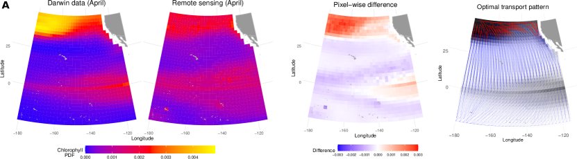
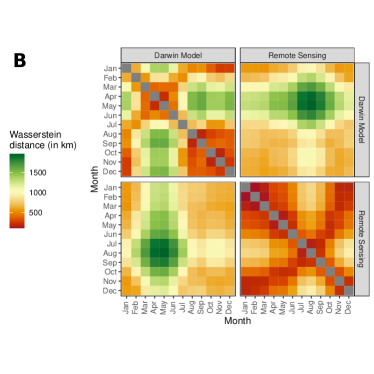
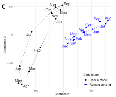
Figure 2: Geographical analysis of Chlorophyll data. Panel A shows a comparison of April’s climatology Chlorophyll maps from two data sources (two left maps) using optimal transport. The first two maps are measurements on a two-dimensional grid in which each grid cell measurement can be thought of as a pixel intensity in a digital image. The values have been normalized to sum to 1 in each map. The third map in Panel A shows the pixel-wise difference (which is the basis for root-mean-squared error—RMSE) of the two left maps. The rightmost map shows the estimated optimal transports (which is the basis for Wasserstein distance), with transparent blue arrows and opaque red lines showing the bottom 90% and top 10% of all the masses, respectively. This mass transfer plot shows that the major shift of Chlorophyll probability mass from the concentrated upper left corner is dispersed in a south- and east-bound direction with a particular trend. Panel B shows a summary of all pairwise Wasserstein distances from the $24$ maps—twelve months of climatology Chlorophyll maps, from the two data sources (model and remote sensing), as a $24\times 24$ distance matrix. Panel C shows a classical multidimensional scaling (MDS) performed on this data. Three notable observations can be made: (1) model data is more variable than remote sensing data, (2) there is a clear separation between model and remote sensing data, and (3) the connecting dashed line between adjacent months in each data source shows an annual seasonality. This is further explored in 3 and Figures S4 and by analyzing data from each year.

(ii) Interannual Variability and Long-term Trends

We expand the analysis by using time-resolved data based on monthly averages of model and remote sensing data in all months available from 1998 to 2006. An MDS analysis leads to similar conclusions as those from the climatology data (see Supplemental Section S1(b) for a detailed analysis). Next, Figure 3 plots the Wasserstein distance between pairs of maps from within a single source (model or remote sensing) as a function of the number of months they are apart. The blue line shows a regression mean that explicitly models annual seasonality, and the red line is the linear trend without the seasonality. The regression model predicts $\sqrt{D_{ab}}$ between year-month $a$ and $b$, using two types of predictors: (i) the number of months apart $|\mathrm{ym}(a)-\mathrm{ym}(b)|$ that includes year information and the (ii) number of calendar months apart if one ignores the years, i.e. $|\mathrm{m}(a)-\mathrm{m}(b)|\in\{0,\ldots,6\}$. The predictor in (ii) is an explicit accounting for differences in the time of year. In particular, the fitted model for $\sqrt{D_{ab}}$ shown by the blue line is given by

$$\hat{\beta}_{0}+\hat{\beta}_{1}\cdot|\mathrm{ym}(a)-\mathrm{ym}(b)|+\sum_{k=0}^{6}\hat{\beta}_{2,k}\mathds{1}(|\mathrm{m}(a)-\mathrm{m}(b)|=k),$$ (2)

where $\sum_{k=0}^{6}\hat{\beta}_{2,k}=0$. The red line is simply the first two terms of the above expression. The undulating blue line indicates the larger seasonal variability in Chlorophyll patterns in the model relative to remote sensing data noted in Section 3(a)(i). The slope of the red line, $\hat{\beta}_{1}$, is positive for remote sensing and 8.5 times that of the model data. Indeed, the upward trend of the red line for the remote sensing data is visibly much more apparent than that for the model data. This suggests that the Chlorophyll maps in the remote sensing data are getting increasingly more different from each other (i.e. there is a trend in the Chlorophyll patterns) in a way that is not reflected in the model. This is further supported by Figure S5 that shows a sustained trend in the remote sensing data over a longer time period (1996-2020), as well as by the MDS plots in Figure S6. Using RMSE instead of Wasserstein distance in Figure S7, the increasing trend is weaker but still present, and about 2 times larger in remote sensing data than in model data.

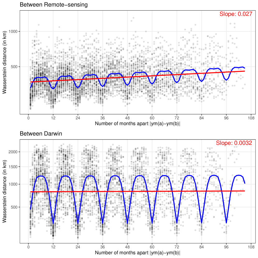
Figure 3: Wasserstein distance between time-resolved Chlorophyll data from different months (between March 1998 to December 2006) for the remote sensing (Panel A) and model (Panel B) data, arranged so that the $x$-axis shows how many months apart the two Chlorophyll maps are, and the $y$-axis is the Wasserstein distance (which uses square-root scaling). The blue line is fitted using a regression model that assumes a linear trend together with a regular seasonal pattern, and the red line shows the linear trend excluding the seasonal component. The slope of the red line for the remote sensing data is roughly $8.4$ times larger than for the model data – both slope values are shown in the top-right of each panel. Note, the red line is linear in $\sqrt{D_{ab}}$, and only appears linear here because the slope coefficient is very small in size.

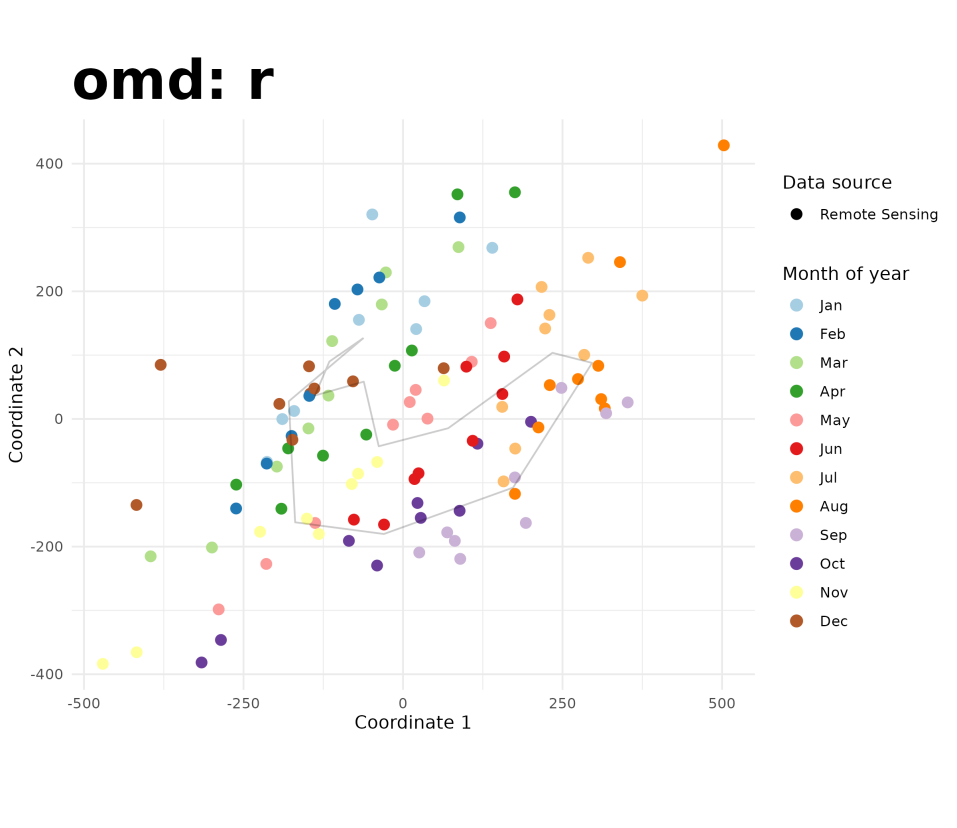
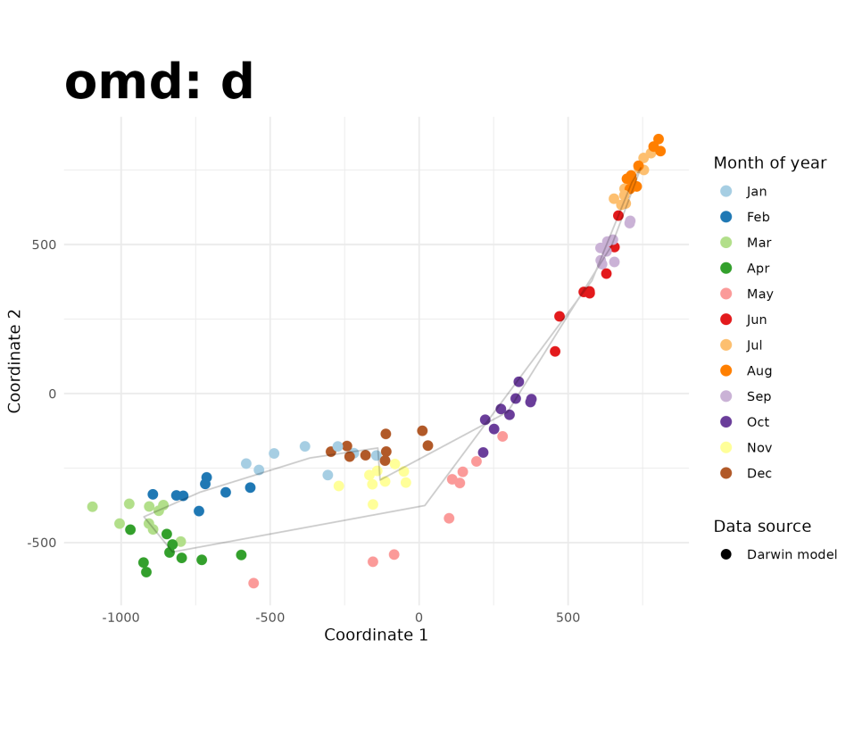
Figure 4: Separate MDS plots created from the two data sources. (Figure  shows the MDS plot created from both sources together.) The top panel uses remote sensing, and the bottom panel uses Darwin data.

Lastly, Figure 4 highlights a stark contrast between Wasserstein distance and RMSE. The lines plotted in Panel A show the distance from model data in January 1998 to all other months of model data in our date range, measured in two ways (Wasserstein distance and RMSE). Both have regular seasonality, but the Wasserstein distance curve peaks in the summer (around August) of each year, while the RMSE curve peaks in the early Spring (around April). We focus on three months—shown as January 1998 (I), April 2002 (II), and August 2002 (III) in Panel A—and note that the domain of calculations have been extended further northward as compared with Figure 2.

In Panel B comparing (I) and (II), we see that the RMSE is relatively high due to a few large mismatches in the coastal region, while the Wasserstein distance in this comparison is relatively small because only local shifts exist in the North. On the other hand, Panel C comparing (I) and (II) shows that Wasserstein distance is appropriately large; the rightmost figure shows how optimal transport captures many global south-bound shifts in probability mass to the equatorial region. Pixel-wise difference (third figure from the left) fails to capture this visibly large pattern difference, and RMSE is measured to be smaller than from the comparison in Panel B. This demonstrates how Wasserstein distance can be an improvement over RMSE in quantifying such differences between maps.

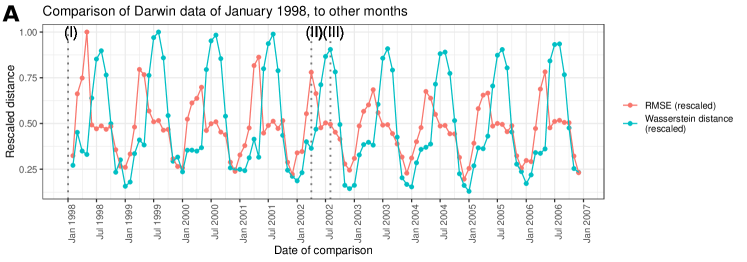
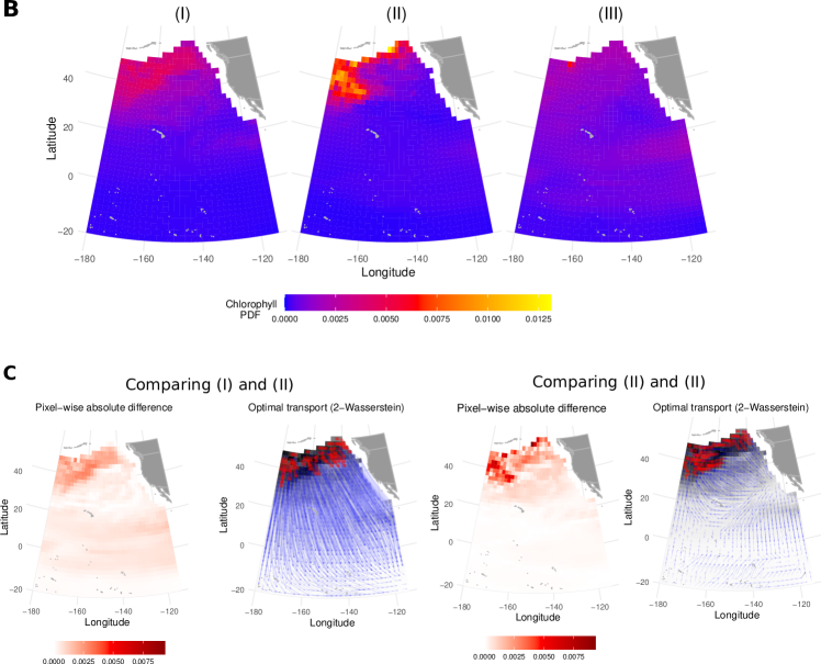
Figure 4: Comparison between the interpretation of time series data using Wasserstein distance and root-mean-squared error (RMSE). Panel A shows the distance between January 1998 model data (I) to other months’ model data, measured by Wasserstein distance and RMSE, with distances normalized to range from 0 to 1. Panel B shows the three maps. Noticing that the seasonal cycle and annual peak of Wasserstein distance is different in the two sources, we focused on two months—April 2002 (II) when RMSE peaks and Aug 2002 (III) when Wasserstein distance peaks. (Grey vertical dotted lines are drawn at dates (I), (II), and (III) for emphasis.) RMSE measures January to be more different from April than it is from August, while Wasserstein distance measured the opposite. In panel C, the optimal transport between (I) and (II) is mostly short shifts locally in the north, while the pixel-wise difference is overly pronounced due to a few large differences in the northern coastal region. On the other hand, the optimal transport between (I) and (III) includes two types of shifts—those that are local to the northern region, and sizeable equator-bound shifts. The pixel-wise difference does not capture the latter. Note, only half of the arrows are shown in the optimal transport plots for visual clarity. The year of $2002$ was chosen randomly, and the same analysis using another comparison year shows similar conclusions.

(iii) Comparing Ocean Provinces

Sometimes, rather than comparing the scalar fields directly, we may be more interested in comparing a scientifically relevant derived feature of the fields. For example, one may algorithmically segment the ocean into cohesive regions—”provinces”—based on underlying differences in one or more fields (e.g. Kavanaugh et al. (2014); Oliver and Irwin (2008); Sonnewald et al. (2020); Wüst et al. (2020).

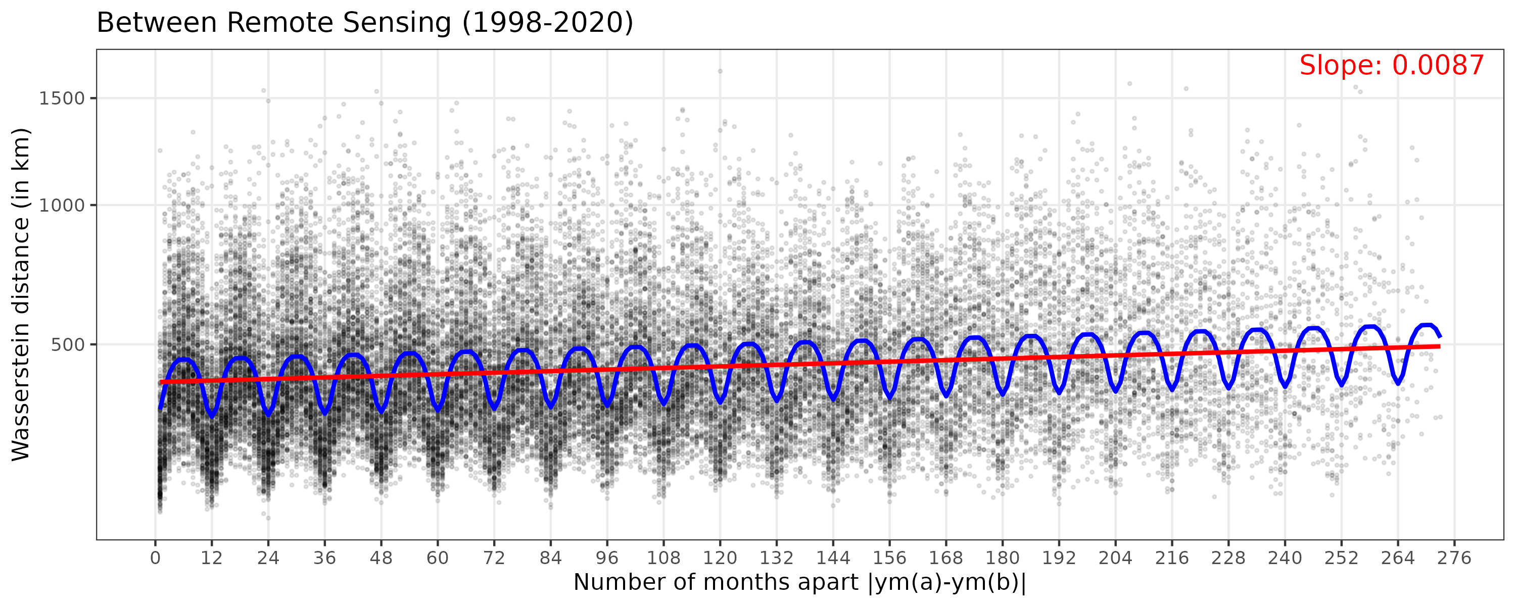
Figure 5: In the same style as Figure 3, we show the Wasserstein distance between Chlorophyll data from different months in a longer time range than before—between March 1998 to December 2020. This plot is arranged so that the $x$-axis shows how many months apart the two Chlorophyll maps are, and the $y$-axis is the Wasserstein distance (logarithmically spaced). In an estimated regression model (2), the blue line shows an estimate as a function of time apart, and the red line shows an increasing linear trend. This additionally supports the conclusion from 3 that the further away the two months are, the larger the OMD between their Chlorophyll maps is. The slope of the red line is $0.0087$, which is about $3.7$ times larger than the slope from Darwin simulation data.

We show here how Wasserstein distance can be used to evaluate how different the boundaries are of such provinces when determined from different datasets or algorithms. Here, we apply a clustering algorithm (K-means clustering) to two Chlorophyll maps—one from remote sensing and the other from the model—to estimate two different spatial provinces of Chlorophyll. In our study region, this province boundary occurs in the North Pacific Transition Zone and is often referred to as the Transition Zone Chlorophyll Front (TZCF) Polovina et al. (2000); Follett et al. (2021). We demonstrate in this section how to use Wasserstein distance to flexibly measure the difference between ocean provinces, by measuring how much transport is needed to move the boundaries of one set of provinces (based on model data) to make them equivalent to that of an alternative definition of provinces (based on remote sensing data). Given a partition of the ocean, we can extract a binary scalar field that is 0 inside the provinces and equal to a nonzero constant along the discretized boundaries between regions. Given two such binary scalar fields, we can then apply Wasserstein distance. An example is shown in Panel A of Figure 5 for the March and August Chlorophyll climatologies, where the estimated boundary is shown as yellow (model) and blue (remote sensing) lines.

It is interesting to compare the distance matrices (Panels B) and the MDS plots (Panels C) in Figure 5 and Figure 2, which was formed by applying Wasserstein distance to the Chlorophyll field itself. When performing Wasserstein distance on the boundaries, the MDS plot in Figure 5 shows little between-source difference (compared to within-source seasonal variability), with the months from the two data sources lining up with each other. By contrast, the MDS plot of Figure 2 showed a larger degree of between-source variability. In other words, despite the relatively large between-source distance between Chlorophyll maps, we see that in terms of one important aspect—the estimated boundary between the regions—the two data sources agree rather well. Putting this in the context of data source comparison, boundary comparison show a much better connection between the model and remote sensing data than the Chlorophyll fields themselves, suggesting the model captures the overarching patterns and controls although not the exact locations and more detailed patterns.

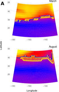
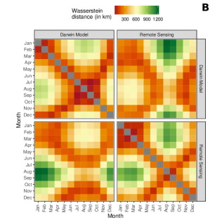
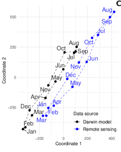
Figure 5: Comparison of ocean provinces using Wasserstein distance ($W_{2}$). Panel A shows an example of the application of Wasserstein distance on cluster boundaries for March and August based on Chlorophyll climatology data (the full set of plots from all months are provided in Figure S8). The plots show province boundaries estimated from remote sensing (blue line) and model (yellow line) data, overlaid on model Chlorophyll data shown as heatmaps. The next two panels show summaries of all pairwise Wasserstein distances from the $24$ maps of estimated cluster boundaries (for the twelve months of climatology Chlorophyll maps from the two sources) in the same style as Figure 2. Panel B shows a $24\times 24$ distance matrix, and Panel C shows a classical multidimensional scaling (MDS) performed on this data. The distance between the two data sources in the same month is small and the seasonal dynamic shown by the lines is similar in the two data sources. This shows that, despite the large between-source distance between Chlorophyll maps in 2, one important aspect—the estimated boundary between the two bodies of water (the North Pacific Transition Zone and the Subtropical Gyre)—is similar between the two data sources.

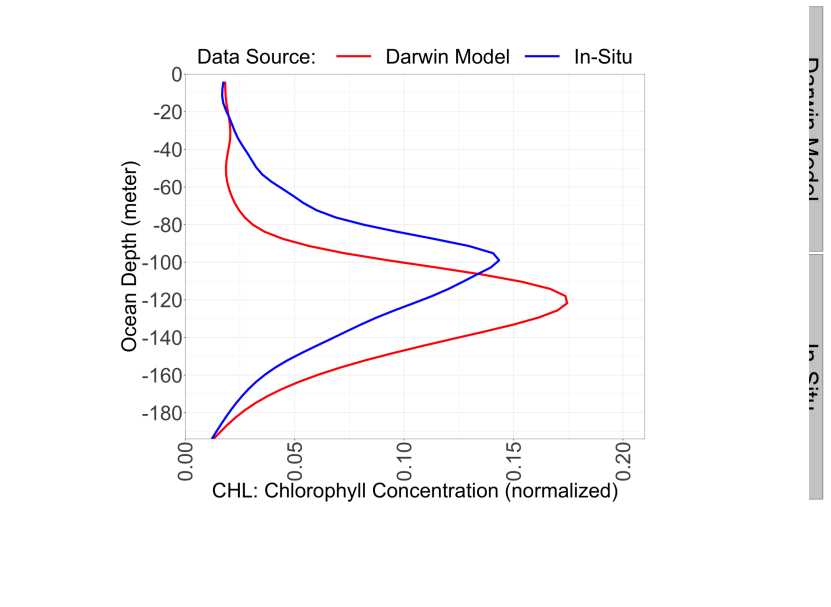
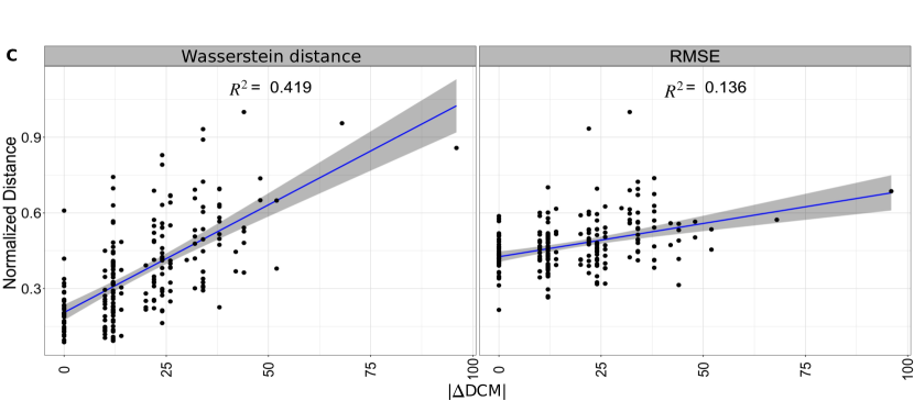
Figure 6: Comparing depth profiles of Chlorophyll from to data sources. Panel A and B show depth profiles of Chlorophyll from two data sources—model and in situ—with an example of a single depth profile for 2013-09-15 given in Panel A and all depth profiles between October 1988 and November 2016 (n = 226) given in Panel B. Each vertical slice (a single 1-dimensional histogram of Chlorophyll distribution from each data source) at overlapping time points can be compared using Wasserstein distance ($W_{2}$). Panel C shows the effectiveness of the two distance measures, root-mean-square error (RMSE) and Wasserstein distance ($y$-axis), in capturing the difference in the deep Chlorophyll maximum (DCM: $x$-axis) recorded from the model and at Station ALOHA (in situ) at shared dates. DCM refers to the region below the ocean surface where the maximum concentration of Chlorophyll is observed. The higher $R^{2}$ demonstrates that Wasserstein distance is better able to capture the variability in the difference in the DCM than RMSE.

(b) Comparing Depth Profiles of Chlorophyll

In this section, we use Wasserstein distance to compare Chlorophyll depth profiles at Station ALOHA using two different data sources (in situ and model). In the vertical profile of Chlorophyll, a Deep Chlorophyll Maximum (DCM) (sometimes also referred to as a Subsurface Chlorophyll Maximum, SCM Anderson (1969)) is observed as a pronounced peak at depth (generally below the first optical depth) (Figure 6). A DCM develops under stratified conditions Estrada et al. (1993) at the point of cross-over between two conditions that limit phytoplankton growth. Surface waters are light-rich and nutrient-limited, while at depth nutrient concentrations are high and photosynthesis is light-limited Dugdale (1967); Hodges and Rudnick (2004). At the depth of cross-over between these conditions a DCM can develop Steele and Yentsch (1960); Beckmann and Hense (2007); Cullen (2015) and the consumption of nutrients by phytoplankton acts to fix this DCM at a given depth.

Figure 6 shows Wasserstein distance and RMSE comparisons between Chlorophyll depth profiles from two data sources—in situ and model—at 226 shared dates between October 1988 and November 2016. Panel A shows an example of a single Chlorophyll depth profile for the two data sources (for 2014-09-15), while all 226 depth profiles for each data source are shown in Panel B. For each comparison (i.e. each common date), we also record an estimate of the DCM, measured by the depth at which the maximum concentration of Chlorophyll occurs. Panel C shows linear regressions of Wasserstein distance and RMSE on the estimated difference in DCM between the two data sources. The higher $R^{2}$ of the left panel of Figure 6C suggests that Wasserstein distance is more effective than RMSE at capturing the observed difference in DCM. Additionally, Figure S9 shows that the most prominent movement across depth—pooled across all comparisons made—is from approximately 96 meters in the in situ data, to 140 meters in model data. This indicates that in aggregate, there is a depth-wise mismatch in the DCM between the two data sources. Wasserstein distance uncovers the spatial mismatch without the additional step of isolating the DCM.

4. Conclusion

We have demonstrated through a series of examples how Wasserstein distance can be a useful tool for oceanographers performing the common task of comparing scalar fields in the ocean. Our analyses focused on two time-varying Chlorophyll datasets in the Pacific Ocean—a map defined over a longitude-latitude box in the North Pacific and a depth profile at Station ALOHA. In several examples, we found that Wasserstein distance was able to capture differences in seasonality, distribution shifts, and other scientifically-relevant factors in ways that a pixel-wise difference could not. For example, in the depth profile analysis, Wasserstein distance could more closely track the changes in the deep Chlorophyll maximum than RMSE. A further advantage over RMSE that we did not demonstrate in our examples is that Wasserstein distance does not require the two sources to be defined on identical sets of spatial cells.

Our Wasserstein distance-based analysis also suggested that the differences in Chlorophyll data from the model and remote sensing observations can sometimes be larger than the within-source seasonal variability. The optimal transport maps that are generated in the computation of Wasserstein distance allowed us to understand that this difference was driven by a seasonally varying set of global-scale probability mass shifts. We also found that a key feature of these two data sources—the estimated boundary between the subpolar zone and the subtropical gyre—are much more similar in this region than the original Chlorophyll maps. Analysis of Wasserstein distance on remote sensing data (further analyzed with a linear regression with customized covariates) also helped reveal a long-term change from 1998 to 2006 that is not present in the model data. This suggests the usefulness of Wasserstein distance for examining spatial data over time within a single source. Current studies often establish long-term trend terms of changes in magnitude; Wasserstein distance detects changes in patterns, which may help detect long-term trends efficiently and with less uncertainty.

The demonstrations within this paper are just a starting point for the potential uses of the Wasserstein distance. We envisage this metric being used by many oceanographic data scientists for a variety of comparisons, across a range of dimensions and variables. One particular future development of interest would build on our application of Wasserstein distance to province boundaries with exploration of this technique for more complex applications than the single horizontal TZCF boundary demonstrated here. Defining and testing provinces (“biomes”) in the ocean is an active area of research Wüst et al. (2020); Sonnewald et al. (2020), and we believe that Wasserstein distances can provide a flexible tool to compare competing definitions of biomes.

As demonstrated in our examples, Wasserstein distance is particularly useful for model-data comparison because models can struggle to get the physical location of some key features in the ocean, such as the Gulf Stream. A pixel-wise comparison will measure the magnitude of difference at rigid locations, while Wasserstein distance will focus on the pattern change and appropriately measure this discrepancy in the longitude-latitude space.

Further, the regression analysis in Section 3a(ii) suggests Wasserstein distance as a powerful tool to examine temporal trends in patterns rather than in magnitudes. This shows Wasserstein distance goes far beyond simple model-data comparison, and can be useful for analyzing spatial fields of ocean physical, biogeochemical as well as optical quantities over time.

Developing computational improvements will be important to allow for full global ocean comparisons. One simple extension is to only allow local transports, by directly modifying the base distances. Handling this sparser structured base distance effectively—by building specialized software—may be an important practicality. Faster approximations to optimal transport are popular in computer science and machine learning applications, and can also be adopted when analyzing ocean data.

Another methodological extension is to consider optimal transport with unequal masses Chizat et al. (2016), a natural scenario when dealing with physical quantities in the ocean. Normalizing such data prior to analysis discards a potentially important piece of information, which is the total amount of mass prior to normalization. When the data in a few bins are very large, the normalization can unduly flatten the probability mass in other bins. An interesting future direction is to allow optimal transport to borrow from physical transport to become more physically realistic. Optimal transport is not to be confused with physical transport of the underlying quantity in the ocean. Instead, optimal transport can be thought of as an alternative measure of distance that measures pattern shifts in the space of the data. Nonetheless, making the optimal transport more physically constrained could be a beneficial future direction. To do so, one could adjust the base distance $d_{ij}$ to account for factors such as natural boundaries in the ocean (e.g. two clear bodies of water that do not mix) or ocean currents that prevent or promote movement in certain directions. For example, by simulating Lagrangian drifts of particles under known currents one might be able to form a more oceanographically relevant base distance that is then inputted into the Wasserstein distance calculation.

Data and code. Available in https://github.com/sangwon-hyun/omd.

Author contributions. BJ and GF contributed to data curation. SH, AM, CLF, and JB contributed to formal analysis. CM and JB contributed to funding acquisition. SH, AM, CLF, CM, and JB contributed to investigation and methodology. SH, CLF, and JB contributed to project administration. SH, AM, and BJ contributed to software. JB and CM contributed to supervision. SH, AM, and GF contributed to validation and visualization. All authors contributed to writing (both original draft, review and editing)

Competing interests. We have no competing interests.

Funding. This work was supported by grants by the Simons Collaboration on Computational Biogeochemical Modeling of Marine Ecosystems/CBIOMES (Grant ID: 549939 to JB; 827829 and 553242 to CLF; 549931 to MF;// ). Dr. Jacob Bien was also supported in part by NIH Grant R01GM123993 and NSF CAREER Award DMS-1653017. Thomas Jackson was also supported by the National Centre for Earth Observations of the UK. M-F Racault was also partially funded by the “Frontiers of instability in marine ecosystems and carbon export (Marine Frontiers) [NE/V011103/1]”.

Acknowledgements. The authors acknowledge the Center for Advanced Research Computing (CARC) at the University of Southern California for providing computing resources that have contributed to the research results reported within this publication. URL: https://carc.usc.edu.

S1. Supplement

S1(a) Classical Multidimensional Scaling (MDS) Derivation

The classical MDS solution $\hat{Z}$ is obtained by the following steps:

1. Calculate the matrix of squared distances, $D_{2}$, as $(D_{2})_{ij}=D_{i,j}^{2}$.

2. Take the eigen-decomposition of the doubly centered Gram matrix $B=-\frac{1}{2}CD_{2}C=V\Lambda V^{T}$, where $C=I_{N}-N^{-1}1_{N}1_{N}^{T}$ is the centering matrix ($I_{N}$ is an $N\times N$ identity matrix and $1_{N}$ is a vector of ones).

3. Take $\Lambda_{1:2}$, the $2\times 2$ diagonal matrix of the first two positive eigenvalues of $B$. (Note, classical MDS is only possible when at least two positive eigenvalues exist). Take $V_{1:2}$ to be the two-column matrix of the corresponding two eigenvectors of $B$.

Then, the solution is $\hat{Z}=D_{1:2}\Lambda_{1:2}^{1/2}V_{1:2}^{T}$ is a $2$-column matrix whose rows are the desired $2$-dimensional coordinates.

S1(b) Distance Matrix and MDS of All Monthly Data (1998-2006)

Distance matrix.

Continuing from Section 3(a)(ii), the entire Wasserstein pairwise distance matrix in all months in 1998 through 2020 from two sources (remote sensing and Darwin) are shown in Figure S1. The counterpart RMSE distance matrix is in Figure S2.

MDS results.

In the MDS plots in Figure S3 and S4, we can see clear seasonality within each source by following the two closed loops of the grey lines that connect the average coordinates of each month from each source. Furthermore, we observe that the same months from the different years cluster together—the same color points with the same shape cluster together. As with climatology data, Darwin data has a higher variance than remote sensing data. The distance between the two point types (circle and triangle) that are in the same month (same color) is far greater than the distance within each type, supporting the same conclusion as before with the climatology data—that the between-source variability is larger than the within-source variability.

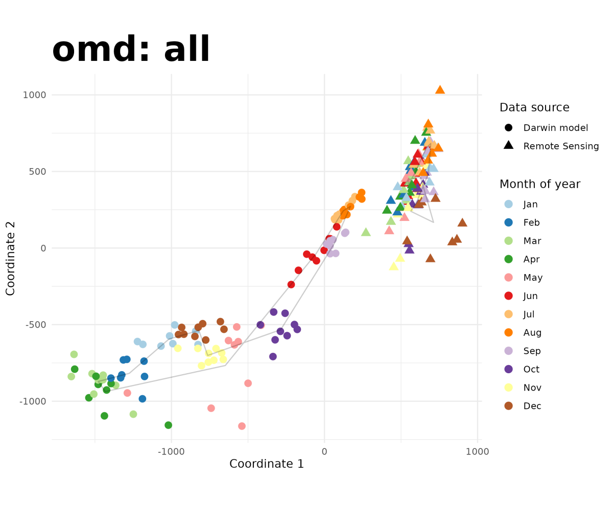
Figure 3: Classical multi-dimensional scaling (MDS) performed using the distance matrix from Figure S1, where each month from each data source is plotted with two shapes—triangles for remote sensing and dots for Darwin model data—and colored by month of year. One plot for each year in 1998-2002. The same months (points with the same color) are clustered, which demonstrates the similarity of Chlorophyll maps from particular month and data source. For each data source, the grey line connects the average coordinate of all years within a month, and form two loops, which shows the seasonality in the two data sources. Figure 4 shows MDS plots produced separately from the two sources.

S1(c) Long-term Change of Chlorophyll Maps

We find a long term temporal trend of Remote sensing Chlorophyll data in two ways—using a specific regression model of the Wasserstein distances (Figure S5, analyzed using the regression model in (2)), and also using a classical MDS of remote sensing Chlorophyll data (Figure S6). The latter analysis is done by examining the MDS of the monthly remote sensing data in 1998-2020 by plotting each month as separate panels. We can see a general drift over the years in the following way. In each panel, each point represents a unique month in this time period, and the point labels are the last two digits of the four-digit year number. The size of the label is smaller for earlier years and larger for later years. We can see that in most years, there is an overall increase along the diagonal direction, from top-right to bottom-left.

S1(d) RMSE Instead of Wasserstein distance in Trend Plot

Figure S7 shows the same method used in Figure 3 but measured using RMSE.

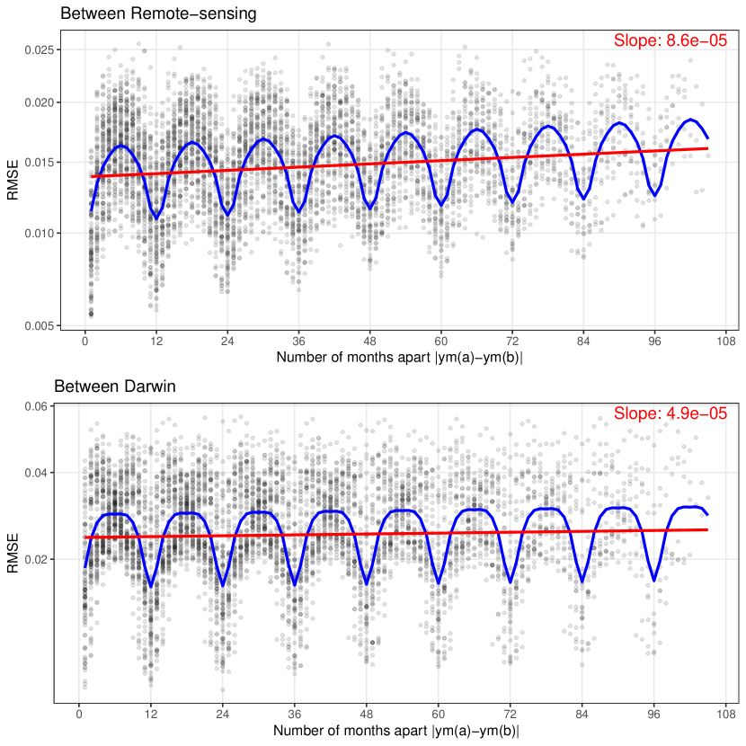
Figure 7: Continuing from Figure 3 (which shows Wasserstein distance), this shows RMSE between Chlorophyll data from all months between March 1998 to December 2006 (for the remote sensing (top panel) and model (bottom panel) data), arranged so that the $x$-axis shows how many months apart the two Chlorophyll maps are, and the $y$-axis is the Wasserstein distance (logarithmically spaced). The blue line is a regression estimate that explicitly accounts for seasonality (in the number of calendar months apart), and the red line is the long-term trend line excluding this seasonality. The slope for remote sensing data is positive and about 2 times larger than for Darwin data.

S1(e) All Boundary Estimates

Figure S8 shows all the boundary estimates in all months of climatology data from the two sources (Darwin and remote sensing), of which a subset was shown in Section 3(a)(iii).

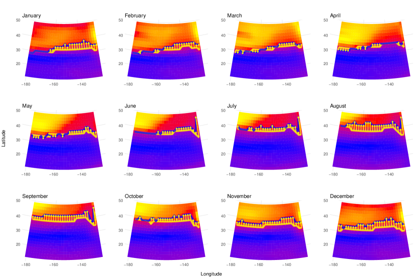
Figure 8: In each of the twelve months of climatology data, the twelve panels show province boundaries estimated from Chlorophyll maps from two sources (remote sensing and Darwin), shown as yellow (Darwin) and blue (remote sensing) lines overlaid on Darwin Chlorophyll data shown as heatmaps. The province boundaries were estimated using a 2-cluster K-means clustering algorithm applied to vertical slices of each dataset. Then, optimal transports between two province boundary maps—with constant mass placed on the boundaries, and zero otherwise—are calculated.

S1(f) Additional Depth Analysis

Additional depth analysis of Chlorophyll is shown in Figure  S9.

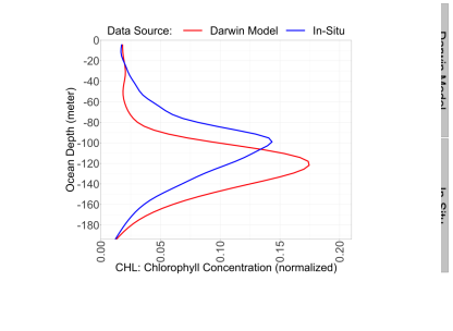
Figure 9: This plot reports the aggregated probability mass transferred from depth profiles in the Darwin model data to the remote sensing data using optimal transport, from all comparisons on all shared dates. See Figure 6 for full analysis.

References

- Dutkiewicz et al. [2015] S Dutkiewicz, A E Hickman, O Jahn, W W Gregg, C B Mouw, and M J Follows. Capturing optically important constituents and properties in a marine biogeochemical and ecosystem model. Biogeosciences, 12(14):4447–4481, 2015. ISSN 17264189. doi: 10.5194/bg-12-4447-2015. URL www.biogeosciences.net/12/4447/2015/.
- Forget et al. [2015a] G. Forget, J.-M. Campin, P. Heimbach, C. N. Hill, R. M. Ponte, and C. Wunsch. Ecco version 4: an integrated framework for non-linear inverse modeling and global ocean state estimation. Geoscientific Model Development, 8(10):3071–3104, 2015a. doi: 10.5194/gmd-8-3071-2015.
- Moore et al. [2009] Timothy S. Moore, Janet W. Campbell, and Mark D. Dowell. A class-based approach to characterizing and mapping the uncertainty of the MODIS ocean chlorophyll product. Remote Sensing of Environment, 113(11):2424–2430, November 2009. doi: 10.1016/j.rse.2009.07.016. URL https://doi.org/10.1016/j.rse.2009.07.016.
- Jackson et al. [2017] Thomas Jackson, Shubha Sathyendranath, and Frédéric Mélin. An improved optical classification scheme for the ocean colour essential climate variable and its applications. Remote Sensing of Environment, 203:152–161, December 2017. doi: 10.1016/j.rse.2017.03.036. URL https://doi.org/10.1016/j.rse.2017.03.036.
- Dutkiewicz et al. [2019] Stephanie Dutkiewicz, Anna E. Hickman, Oliver Jahn, Stephanie Henson, Claudie Beaulieu, and Erwan Monier. Ocean colour signature of climate change. Nature Communications, 10(1), 2019. ISSN 20411723. doi: 10.1038/s41467-019-08457-x. URL https://www.nature.com/articles/s41467-019-08457-x.
- Seegers et al. [2018] Bridget N Seegers, Richard P Stumpf, Blake A Schaeffer, Keith A Loftin, and P Jeremy Werdell. Performance metrics for the assessment of satellite data products: an ocean color case study. Optics express, 26(6):7404–7422, 2018.
- Forget and Ponte [2015] Gaël Forget and Rui M. Ponte. The partition of regional sea level variability. Progress in Oceanography, 137:173–195, 2015. ISSN 0079-6611. doi: 10.1016/j.pocean.2015.06.002.
- Forget et al. [2015b] G. Forget, D. Ferreira, and X. Liang. On the observability of turbulent transport rates by argo: supporting evidence from an inversion experiment. Ocean Science, 11(5):839–853, 2015b. doi: 10.5194/os-11-839-2015. URL https://os.copernicus.org/articles/11/839/2015/.
- Forget and Wunsch [2007] Gaël Forget and Carl Wunsch. Estimated global hydrographic variability. Journal of Physical Oceanography, 37(8):1997–2008, August 2007. doi: 10.1175/jpo3072.1. URL https://doi.org/10.1175/jpo3072.1.
- Forget [2010] Gaël Forget. Mapping ocean observations in a dynamical framework: A 2004–06 ocean atlas. Journal of Physical Oceanography, 40(6):1201–1221, June 2010. doi: 10.1175/2009jpo4043.1. URL https://doi.org/10.1175/2009jpo4043.1.
- Speer and Forget [2013] Kevin Speer and Gael Forget. Chapter 9 - global distribution and formation of mode waters. In Gerold Siedler, Stephen M. Griffies, John Gould, and John A. Church, editors, Ocean Circulation and Climate, volume 103 of International Geophysics, pages 211–226. Academic Press, 2013. doi: https://doi.org/10.1016/B978-0-12-391851-2.00009-X. URL https://www.sciencedirect.com/science/article/pii/B978012391851200009X.
- Cael et al. [2018] BB Cael, Kelsey Bisson, and Christopher L Follett. Can rates of ocean primary production and biological carbon export be related through their probability distributions? Global biogeochemical cycles, 32(6):954–970, 2018.
- Ashkezari et al. [2016] Mohammad D. Ashkezari, Christopher N. Hill, Christopher N. Follett, Gaël Forget, and Michael J. Follows. Oceanic eddy detection and lifetime forecast using machine learning methods. Geophysical Research Letters, 43(23):12,234–12,241, 2016. doi: https://doi.org/10.1002/2016GL071269. URL https://agupubs.onlinelibrary.wiley.com/doi/abs/10.1002/2016GL071269.
- McCaffrey et al. [2015] Katherine McCaffrey, Baylor Fox-Kemper, and Gael Forget. Estimates of ocean macroturbulence: Structure function and spectral slope from argo profiling floats. Journal of Physical Oceanography, 45(7):1773–1793, July 2015. doi: 10.1175/jpo-d-14-0023.1. URL https://doi.org/10.1175/jpo-d-14-0023.1.
- ioc [2020] Synergy between ocean colour and biogeochemical/ecosystem models, 2020.
- Villani [2021] C. Villani. Topics in Optimal Transportation. Graduate Studies in Mathematics. American Mathematical Soc., 2021. ISBN 9781470467265. URL https://books.google.com/books?id=NElDEAAAQBAJ.
- Rubner et al. [2000] Yossi Rubner, Carlo Tomasi, and Leonidas J. Guibas. The earth mover’s distance as a metric for image retrieval. International Journal of Computer Vision, 40(2):99–121, 2000. URL https://doi.org/10.1023/A:1026543900054.
- Nooteboom et al. [2020] Peter D. Nooteboom, Philippe Delandmeter, Erik van Sebille, Peter K. Bijl, Henk A. Dijkstra, and Anna S. von der Heydt. Resolution dependency of sinking lagrangian particles in ocean general circulation models. PLOS ONE, 15(9):e0238650, September 2020. doi: 10.1371/journal.pone.0238650. URL https://doi.org/10.1371/journal.pone.0238650.
- Vissio et al. [2020] Gabriele Vissio, Valerio Lembo, Valerio Lucarini, and Michael Ghil. Evaluating the performance of climate models based on wasserstein distance. Geophysical Research Letters, 47(21), October 2020. doi: 10.1029/2020gl089385. URL https://doi.org/10.1029/2020gl089385.
- Tamang et al. [2020] Sagar K. Tamang, Ardeshir Ebtehaj, Dongmian Zou, and Gilad Lerman. Regularized variational data assimilation for bias treatment using the wasserstein metric. Quarterly Journal of the Royal Meteorological Society, 146(730):2332–2346, April 2020. doi: 10.1002/qj.3794. URL https://doi.org/10.1002/qj.3794.
- Le et al. [2021] Phong V. V. Le, Clément Guilloteau, Antonios Mamalakis, and Efi Foufoula-Georgiou. Underestimated MJO variability in CMIP6 models. Geophysical Research Letters, 48(12), June 2021. doi: 10.1029/2020gl092244. URL https://doi.org/10.1029/2020gl092244.
- Papadakis [2015] Nicolas Papadakis. Optimal transport for image processing. signal and image processing. Habilitation thesis, 2015.
- Colin et al. [2021] Aurelien Colin, Charles Peureux, Romain Husson, Nicolas Longepe, Regis Rauzy, Ronan Fablet, Pierre Tandeo, Samir Saoudi, Alexis Mouche, and Gerald Dibarboure. Segmentation of sentinel-1 SAR images over the ocean, preliminary methods and assessments. In 2021 IEEE International Geoscience and Remote Sensing Symposium IGARSS. IEEE, July 2021. doi: 10.1109/igarss47720.2021.9553429. URL https://doi.org/10.1109/igarss47720.2021.9553429.
- Parno et al. [2019] M. D. Parno, B. A. West, A. J. Song, T. S. Hodgdon, and D. T. O'Connor. Remote measurement of sea ice dynamics with regularized optimal transport. Geophysical Research Letters, 46(10):5341–5350, May 2019. doi: 10.1029/2019gl083037. URL https://doi.org/10.1029/2019gl083037.
- Follett et al. [2021] Christopher L. Follett, Stephanie Dutkiewicz, Gael Forget, B. B. Cael, and Michael J. Follows. Moving ecological and biogeochemical transitions across the North Pacific. Limnology and Oceanography, 9999:lno.11763, 5 2021. ISSN 0024-3590. doi: 10.1002/lno.11763. URL https://onlinelibrary.wiley.com/doi/10.1002/lno.11763.
- Karl and Lukas [1996] David M Karl and Roger Lukas. The hawaii ocean time-series (hot) program: Background, rationale and field implementation. Deep Sea Research Part II: Topical Studies in Oceanography, 43(2-3):129–156, 1996.
- Karl and Church [2014] David M Karl and Matthew J Church. Microbial oceanography and the hawaii ocean time-series programme. Nature Reviews Microbiology, 12(10):699–713, 2014.
- Venrick et al. [1973] EL Venrick, JA McGowan, and AW Mantyla. Deep maxima of photosynthetic chlorophyll in the pacific ocean. Fish. Bull, 71(1):41–52, 1973.
- Cullen [1982] John J Cullen. The deep chlorophyll maximum: comparing vertical profiles of chlorophyll a. Canadian Journal of Fisheries and Aquatic Sciences, 39(5):791–803, 1982.
- Huisman et al. [2006] Jef Huisman, Nga N Pham Thi, David M Karl, and Ben Sommeijer. Reduced mixing generates oscillations and chaos in the oceanic deep chlorophyll maximum. Nature, 439(7074):322–325, 2006.
- Monge [1781] Gaspard Monge. Mémoire sur la théorie des déblais et des remblais. De l’Imprimerie Royale, 1781.
- Kantorovitch [1958] L. Kantorovitch. On the translocation of masses. Management Science, 5(1):1–4, 1958.
- Schuhmacher et al. [2020] Dominic Schuhmacher, Björn Bähre, Carsten Gottschlich, Valentin Hartmann, Florian Heinemann, and Bernhard Schmitzer. transport: Computation of Optimal Transport Plans and Wasserstein Distances, 2020. URL https://cran.r-project.org/package=transport. R package version 0.12-2.
- Bonneel et al. [2011] Nicolas Bonneel, Michiel van de Panne, Sylvain Paris, and Wolfgang Heidrich. Displacement Interpolation Using Lagrangian Mass Transport. ACM Transactions on Graphics (SIGGRAPH ASIA 2011), 30(6), 2011.
- Auricchio et al. [2020] Gennaro Auricchio, Andrea Codegoni, Stefano Gualandi, Giuseppe Toscani, and Marco Veneroni. The equivalence of fourier-based and wasserstein metrics on imaging problems, 2020.
- Shirdhonkar and Jacobs [2008] Sameer Shirdhonkar and David W. Jacobs. Approximate earth mover’s distance in linear time. In 2008 IEEE Conference on Computer Vision and Pattern Recognition, pages 1–8, 2008. doi: 10.1109/CVPR.2008.4587662.
- Cuturi [2013] Marco Cuturi. Sinkhorn distances: Lightspeed computation of optimal transport. In C. J. C. Burges, L. Bottou, M. Welling, Z. Ghahramani, and K. Q. Weinberger, editors, Advances in Neural Information Processing Systems, volume 26. Curran Associates, Inc., 2013. URL https://proceedings.neurips.cc/paper/2013/file/af21d0c97db2e27e13572cbf59eb343d-Paper.pdf.
- Padgham and Sumner [2021] Mark Padgham and Michael D. Sumner. geodist: Fast, Dependency-Free Geodesic Distance Calculations, 2021. URL https://CRAN.R-project.org/package=geodist. R package version 0.0.7.
- Borg and Groenen [2005] I. Borg and P.J.F. Groenen. Modern Multidimensional Scaling: Theory and Applications. Springer, 2005.
- Gower [1966] J. C. Gower. Some distance properties of latent root and vector methods used in multivariate analysis. Biometrika, 53(3/4):325–338, 1966. ISSN 00063444. URL http://www.jstor.org/stable/2333639.
- HOT [2021] HOT. Hydrography https://hahana.soest.hawaii.edu/hot/methods/ctd.html, 2021. URL https://hahana.soest.hawaii.edu/hot/methods/ctd.html.
- Forget [2018] Gael Forget. gaelforget/CBIOMES: Initial, preliminary version of the CBIOMES-global model setup and documentation, August 2018. URL https://doi.org/10.5281/zenodo.1343303.
- Dutkiewicz et al. [2021] Stephanie Dutkiewicz, Philip W. Boyd, and Ulf Riebesell. Exploring biogeochemical and ecological redundancy in phytoplankton communities in the global ocean. Global Change Biology, 27(6):1196–1213, 3 2021. ISSN 13652486. doi: 10.1111/gcb.15493.
- Geider et al. [1998] Richard J. Geider, Hugh L. MacIntyre, and Todd M. Kana. A dynamic regulatory model of phytoplanktonic acclimation to light, nutrients, and temperature. Limnology and Oceanography, 43(4):679–694, 6 1998. ISSN 00243590. doi: 10.4319/lo.1998.43.4.0679. URL http://doi.wiley.com/10.4319/lo.1998.43.4.0679.
- Mélin et al. [2017] F. Mélin, V. Vantrepotte, A. Chuprin, M. Grant, T. Jackson, and S. Sathyendranath. Assessing the fitness-for-purpose of satellite multi-mission ocean color climate data records: A protocol applied to OC-CCI chlorophyll- a data. Remote Sensing of Environment, 203:139–151, December 2017. doi: 10.1016/j.rse.2017.03.039.
- Sathyendranath et al. [2019] Shubha Sathyendranath, Robert Brewin, Carsten Brockmann, Vanda Brotas, Ben Calton, Andrei Chuprin, Paolo Cipollini, André Couto, James Dingle, Roland Doerffer, Craig Donlon, Mark Dowell, Alex Farman, Mike Grant, Steve Groom, Andrew Horseman, Thomas Jackson, Hajo Krasemann, Samantha Lavender, Victor Martinez-Vicente, Constant Mazeran, Frédéric Mélin, Timothy Moore, Dagmar Müller, Peter Regner, Shovonlal Roy, Chris Steele, François Steinmetz, John Swinton, Malcolm Taberner, Adam Thompson, André Valente, Marco Zühlke, Vittorio Brando, Hui Feng, Gene Feldman, Bryan Franz, Robert Frouin, Richard Gould, Stanford Hooker, Mati Kahru, Susanne Kratzer, B. Mitchell, Frank Muller-Karger, Heidi Sosik, Kenneth Voss, Jeremy Werdell, and Trevor Platt. An ocean-colour time series for use in climate studies: The experience of the ocean-colour climate change initiative (OC-CCI). Sensors, 19(19):4285, October 2019. doi: 10.3390/s19194285.
- Sathyendranath et al. [2020] Shubha Sathyendranath, Thomas Jackson, Carsten Brockmann, Vanda Brotas, Ben Calton, Andrei Chuprin, Oliver Clements, Paolo Cipollini, Olaf Danne, James Dingle, Craig Donlon, Michael Grant, Stephen Groom, Hajo Krasemann, Sam Lavender, Constant Mazeran, Frédéric Mélin, Timothy S. Moore, Dagmar Müller, Peter Regner, François Steinmetz, Chris Steele, John Swinton, André Valente, Marco Zühlke, Gene Feldman, Bryan Franz, Robert Frouin, Jeremy Werdell, and Trevor Platt. Esa ocean colour climate change initiative (ocean_colour_cci): Version 4.2 data, 2020. URL https://catalogue.ceda.ac.uk/uuid/d62f7f801cb54c749d20e736d4a1039f.
- Hyun et al. [2019] Sangwon Hyun, Aditya Mishra, and Christian Müller Jacob Bien. Cmap for r users. https://github.com/simonscmap/cmap4r, 2019.
- Kavanaugh et al. [2014] Maria T. Kavanaugh, Burke Hales, Martin Saraceno, Yvette H. Spitz, Angelicque E. White, and Ricardo M. Letelier. Hierarchical and dynamic seascapes: A quantitative framework for scaling pelagic biogeochemistry and ecology. Progress in Oceanography, 120:291–304, January 2014. doi: 10.1016/j.pocean.2013.10.013. URL https://doi.org/10.1016/j.pocean.2013.10.013.
- Oliver and Irwin [2008] Matthew J. Oliver and Andrew J. Irwin. Objective global ocean biogeographic provinces. Geophysical Research Letters, 35(15), August 2008. doi: 10.1029/2008gl034238. URL https://doi.org/10.1029/2008gl034238.
- Sonnewald et al. [2020] Maike Sonnewald, Stephanie Dutkiewicz, Christopher Hill, and Gael Forget. Elucidating ecological complexity: Unsupervised learning determines global marine eco-provinces. Science Advances, 6(22):eaay4740, 2020. ISSN 23752548. doi: 10.1126/sciadv.aay4740. URL https://advances.sciencemag.org/content/6/22/eaay4740?utm_source=TrendMD&utm_medium=cpc&utm_campaign=TrendMD_1.
- Wüst et al. [2020] Eileen Wüst, Simone Zellner, Christian L. Müller, and Fabian Scheipl. Statistical work flows for Marine Data Analysis - Cluster analysis of large-scale ocean data. Statistical consulting report, Department of Statistics, LMU München, November 2020.
- Polovina et al. [2000] Jeffrey J. Polovina, Michael P. Seki, and Evan Howell. Sensors detect biological change in mid-latitude North Pacific. Eos, Transactions American Geophysical Union, 81(44):519, 10 2000. ISSN 0096-3941. doi: 10.1029/00eo00374. URL http://doi.wiley.com/10.1029/00EO00374.
- Anderson [1969] G. C. Anderson. SUBSURFACE CHLOROPHYLL MAXIMUM IN THE NORTHEAST PACIFIC OCEAN1. Limnology and Oceanography, 14(3):386–391, May 1969. doi: 10.4319/lo.1969.14.3.0386. URL https://doi.org/10.4319/lo.1969.14.3.0386.
- Estrada et al. [1993] Marta Estrada, Celia Marrasé, Mikel Latasa, Elisa Berdalet, Maximino Delgado, and Tecla Riera. Variability of deep chlorophyll maximum characteristics in the northwestern mediterranean. Marine Ecology Progress Series, 92(3):289–300, 1993. ISSN 01718630, 16161599. URL http://www.jstor.org/stable/24832534.
- Dugdale [1967] R. C. Dugdale. Nutrient limitation in the sea: Dynamics, identification, and significance1. Limnology and Oceanography, 12(4):685–695, 1967. doi: https://doi.org/10.4319/lo.1967.12.4.0685. URL https://aslopubs.onlinelibrary.wiley.com/doi/abs/10.4319/lo.1967.12.4.0685.
- Hodges and Rudnick [2004] Benjamin A Hodges and Daniel L Rudnick. Simple models of steady deep maxima in chlorophyll and biomass. Deep Sea Research Part I: Oceanographic Research Papers, 51(8):999–1015, 2004. ISSN 0967-0637. doi: https://doi.org/10.1016/j.dsr.2004.02.009. URL https://www.sciencedirect.com/science/article/pii/S0967063704000482.
- Steele and Yentsch [1960] J. H. Steele and C. S. Yentsch. The vertical distribution of chlorophyll. Journal of the Marine Biological Association of the United Kingdom, 39(2):217–226, 1960. doi: 10.1017/S0025315400013266.
- Beckmann and Hense [2007] Aike Beckmann and Inga Hense. Beneath the surface: Characteristics of oceanic ecosystems under weak mixing conditions – a theoretical investigation. Progress in Oceanography, 75(4):771–796, 2007. ISSN 0079-6611. doi: https://doi.org/10.1016/j.pocean.2007.09.002. URL https://www.sciencedirect.com/science/article/pii/S0079661107001826.
- Cullen [2015] John J. Cullen. Subsurface chlorophyll maximum layers: Enduring enigma or mystery solved? Annual Review of Marine Science, 7(1):207–239, 2015. doi: 10.1146/annurev-marine-010213-135111. URL https://doi.org/10.1146/annurev-marine-010213-135111. PMID: 25251268.
- Chizat et al. [2016] Lénaïc Chizat, Gabriel Peyré, Bernhard Schmitzer, and François-Xavier Vialard. An interpolating distance between optimal transport and fisher–rao metrics. Foundations of Computational Mathematics, 18(1):1–44, October 2016. doi: 10.1007/s10208-016-9331-y. URL https://doi.org/10.1007/s10208-016-9331-y.