Phonon-induced rotation of the electronic nematic director in superconducting Bi₂Se₃

Abstract

The doped topological insulator $A_{x}\mathrm{Bi_{2}Se_{3}}$, with $A=\{\mathrm{Cu},\mathrm{Sr},\mathrm{Nb}\}$, becomes a nematic superconductor below $T_{c}\sim 3-4\,\mathrm{K}$. The associated electronic nematic director is described by an angle $\alpha$ and is experimentally manifested in the elliptical shape of the in-plane critical magnetic field $H_{c2}$. Because of the threefold rotational symmetry of the lattice, $\alpha$ is expected to align with one of three high-symmetry directions corresponding to the in-plane nearest-neighbor bonds, consistent with a $Z_{3}$-Potts nematic transition. Here, we show that the nematic coupling to the acoustic phonons, which makes the nematic correlation length tend to diverge along certain directions only, can fundamentally alter this phenomenology in trigonal lattices. Compared to hexagonal lattices, the former possesses a sixth independent elastic constant $c_{14}$ due to the fact that the in-plane shear strain doublet $(\epsilon_{xx}-\epsilon_{yy},-2\epsilon_{xy})$ and the out-of-plane shear strain doublet $(2\epsilon_{yz},-2\epsilon_{xz})$ transform as the same irreducible representation. We find that, when $c_{14}$ overcomes a threshold value, which is expected to be the case in doped $\mathrm{Bi_{2}Se_{3}}$, the nematic director $\alpha$ unlocks from the high-symmetry directions due to the competition between the quadratic phonon-mediated interaction and the cubic nematic anharmonicity. This implies the breaking of the residual in-plane twofold rotational symmetry ($C_{2x}$), resulting in a triclinic phase. We discuss the implications of these findings to the structure of nematic domains, to the shape of the in-plane $H_{c2}$ in $A_{x}\mathrm{Bi_{2}Se_{3}}$, and to presence of nodes inside the superconducting state.

I Introduction

In nematic superconductors, the superconducting transition is accompanied by the breaking of a symmetry of the crystalline lattice. As a result, a nematic pairing state is manifested by substantial anisotropies in thermodynamic quantities such as the upper-critical field ($H_{c2}$), the penetration depth, and the thermal conductivity. Quite generally, a nematic superconducting state requires a multi-component complex order parameter $\boldsymbol{\Delta}=(\Delta_{1},\Delta_{2},\dots)^{T}$. In one scenario, which assumes some degree of fine tuning, the components transform as different one-dimensional irreducible representations (IR) of the point group that order at very close transition temperatures ($T_{c}$) (Chichinadze et al., 2020; Wang et al., 2021). This would be the case, for instance, of an $s+d_{x^{2}-y^{2}}$ state in a tetragonal lattice, which lowers the symmetry of the system to orthorhombic (Fernandes and Millis, 2013; Livanas et al., 2015; Soto-Garrido and Fradkin, 2014). Another scenario, which does not require fine tuning, corresponds to the case in which $\boldsymbol{\Delta}$ transforms as a multi-dimensional IR (Fu, 2014; Hecker and Schmalian, 2018). An example is the $d_{xy}+d_{x^{2}-y^{2}}$ state in a hexagonal lattice, which breaks the sixfold rotational symmetry of the crystal (Su and Lin, 2018; Venderbos and Fernandes, 2018; Kozii et al., 2019; Scheurer and Samajdar, 2020).

Several materials have been found to display signatures of nematic superconductivity, including the family of doped topological insulators $A_{x}\mathrm{Bi_{2}Se_{3}}$, with dopants $A=\{\mathrm{Cu},\mathrm{Sr},\mathrm{Nb}\}$ (Matano et al., 2016; Pan et al., 2016; Asaba et al., 2017); few-layer transition-metal dichalcogenide $\mathrm{Nb_{2}Se}$ (Hamill et al., 2021; Cho et al., 2020a); twisted bilayer graphene (Cao et al., 2021); and iron-pnictide superconductors (Li et al., 2017; Kushnirenko et al., 2020). In this paper, we focus on the $A_{x}\mathrm{Bi_{2}Se_{3}}$ compounds, which form a trigonal lattice with point group $\mathsf{D_{3d}}$. The fact that the superconducting state breaks the threefold rotational symmetry ($C_{3z}$) has been well-established by measurements of the upper critical field $H_{c2}$, the NMR Knight shift, the resistivity, the magnetic torque, the angle-resolved specific heat, the thermal expansion, and by scanning tunneling spectroscopy (Du et al., 2017; Yonezawa et al., 2017; Pan et al., 2016; Tao et al., 2018; Kuntsevich et al., 2018; Shen et al., 2017; Willa et al., 2018; Sun et al., 2019; Kostylev et al., 2020; Nikitin et al., 2016; Smylie et al., 2018, 2017; Asaba et al., 2017; Matano et al., 2016; Cho et al., 2020b; Kuntsevich et al., 2019; Mi et al., 2021; Kawai et al., 2020). The main candidate for this pairing state is the odd-parity “p-wave” $E_{u}$ state, parametrized here by the two-component order parameter $\boldsymbol{\Delta}=(\Delta_{1},\Delta_{2})^{T}$ (Fu, 2014; Das et al., 2020; Smylie et al., 2017; Kriener et al., 2011; Zyuzin et al., 2017; Kuntsevich et al., 2019). The nematic ground state corresponds to $\boldsymbol{\Delta}=\Delta_{0}(\cos\gamma,\,\sin\gamma)^{T}$ with the directions $\gamma\in[0,\pi)$ restricted to two sets of values, each with three possible directions (Venderbos et al., 2016a; Hecker and Schmalian, 2018; How and Yip, 2019). While one set, $\gamma=\frac{\pi}{6}\{0,2,4\}$, results in a fully gapped state, the other set, $\gamma=\frac{\pi}{6}\{1,3,5\}$, generates point nodes. Which of the two sets is realized is still subject of experimental studies that aim at identifying whether or not nodal quasiparticles are present (Das et al., 2020; Kriener et al., 2011; Smylie et al., 2018, 2017).

Using the product decomposition $E_{u}\otimes E_{u}=A_{1g}\oplus A_{2g}\oplus E_{g}$, one identifies two possible real-valued bilinear combinations of $\boldsymbol{\Delta}$ that transform non-trivially under the point-group $\mathsf{D_{3d}}$: the scalar $\Phi^{A_{2g}}=\boldsymbol{\Delta}^{\dagger}\tau^{y}\boldsymbol{\Delta}$, which breaks time-reversal symmetry and vanishes in the nematic ground state, and the two-component order parameter:

[][]

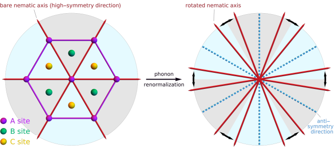
Figure 1: Schematic representation of the electronic nematic director in doped $\mathrm{Bi_{2}Se_{3}}$ compounds. The left panel shows the threefold degenerate nematic directors aligned with the high-symmetry directions of the crystal, superimposed with the unit cell of $\mathrm{Bi_{2}Se_{3}}$. The latter displays a characteristic A-B-C stacking pattern for which, along a particular path along the $z$-direction, the A, B, C lattice sites are either occupied by $\mathrm{Bi}$ or $\mathrm{Se}$ atoms, see e.g. Refs.(Matano et al., 2016; Hecker, 2020). When the coupling to acoustic phonons overcomes a threshold value, two effects occur (right panel): (i) a rotation of the nematic director away from the high-symmetry directions, and (ii) a splitting of the original director into two, which move towards six “anti-symmetry directions”. As a result, the number of non-identical directors doubles from three to six, and the system loses its residual in-plane twofold rotational symmetry $C_{2x}$ inside the nematic phase.

$$\boldsymbol{\Phi}^{E_{g}} =\left(\!\!\begin{array}[]{c}\boldsymbol{\Delta}^{\dagger}\tau^{z}\boldsymbol{\Delta}\\ -\boldsymbol{\Delta}^{\dagger}\tau^{x}\boldsymbol{\Delta}\end{array}\!\!\right)=\left(\!\!\begin{array}[]{c}\Phi^{E_{g},1}\\ \Phi^{E_{g},2}\end{array}\!\!\right)=|\boldsymbol{\Phi}^{E_{g}}|\left(\!\begin{array}[]{c}\cos\alpha\\ \sin\alpha\end{array}\!\right),$$ (7)

which breaks the $C_{3z}$ symmetry of the lattice and is non-zero inside the nematic ground state. Here, the nematic director $\alpha$ is related to $\gamma$ above via $\gamma=-\alpha/2$. Interestingly, fluctuations can cause this bilinear to undergo its own phase transition before the onset of superconductivity (Fernandes et al., 2019), resulting in a narrow sliver of vestigial nematicity above $T_{c}$, as observed experimentally in $A_{x}\mathrm{Bi_{2}Se_{3}}$ (Hecker and Schmalian, 2018; Cho et al., 2020b; Sun et al., 2019).

The bilinear $\boldsymbol{\Phi}^{E_{g}}$ is thus identified as a nematic order parameter, whose “orientation”—encoded in the nematic director $\alpha\in[0,2\pi)$—is directly manifested in properties such as the anisotropy of the in-plane $H_{c2}$ or the direction of elongation (or contraction) of the crystallographic unit cell inside the monoclinic phase. Importantly, the symmetries of the lattice render $\boldsymbol{\Phi}^{E_{g}}$ a $Z_{3}$ (i.e. $3$-state) Potts variable (Hecker and Schmalian, 2018; Xu et al., 2020; Fernandes and Venderbos, 2020; Jin et al., 2021). Consequently, in three dimensions, it is expected to undergo a first-order transition into a threefold degenerate ground state where the director $\alpha=\alpha_{s}$ is aligned with one of the high-symmetry directions of the lattice, $\alpha_{s}\in\{0,2,4\}\frac{\pi}{3}$ or $\alpha_{s}\in\{1,3,5\}\frac{\pi}{3}$, as illustrated in Fig. 1 (left panel). However, experiments have observed an apparent discrepancy between $\alpha$ and $\alpha_{s}$ (Du et al., 2017; Kuntsevich et al., 2018; Tao et al., 2018).

In this paper, we revisit the issue of the orientation of the electronic nematic director in trigonal lattices by considering the coupling to the elastic degrees of freedom. It is well known that when an order parameter couples bilinearly to strain, as it is always the case for nematic order, the low-energy elastic fluctuations (i.e. the acoustic phonons) mediate long-range order-parameter interactions (Cowley, 1976; Folk et al., 1976; Chou and Nelson, 1996). This results in the emergence of non-analytical terms in the susceptibility, implying that the order parameter fluctuations are only soft along certain momentum-space directions (Qi and Xu, 2009; Karahasanovic and Schmalian, 2016; Paul and Garst, 2017; de Carvalho and Fernandes, 2019; Fernandes and Venderbos, 2020). In the context of electronic nematic phases, this important effect has been studied in the cases of tetragonal and hexagonal lattices, where it was shown to promote mean-field behavior at finite temperatures and to suppress non-Fermi liquid behavior near the putative zero-temperature transition. We find that the case of trigonal lattices is qualitatively different, as the nemato-elastic coupling can unlock the nematic director from the high-symmetry directions, resulting in $\alpha\neq\alpha_{s}$ as illustrated in Fig. 1 (right panel). More specifically, the three possible nematic directors split into six, each associated with four momentum-space directions where the nematic fluctuations are the largest.

Formally, this result is a consequence of the competition between a phonon-mediated non-analytic quadratic term in the nematic free energy, which prefers to align $\alpha$ with the “anti-symmetry directions” $\alpha_{as}\in\{1,3,5,7,9,11\}\frac{\pi}{6}$ (i.e. the directions farthest away from the high-symmetry directions), and the intrinsic nematic anharmonic cubic term, which favors $\alpha$ parallel to $\alpha_{s}$. Crucially, the former appears in trigonal lattices, but is absent in hexagonal lattices, although both types of lattices have $C_{3z}$ symmetry. This is because only in trigonal lattices the in-plane shear-strain doublet $\boldsymbol{\epsilon}^{E_{g},1}=(\epsilon_{11}-\epsilon_{22},-2\epsilon_{12})^{T}$ and the out-of-plane shear-strain doublet $\boldsymbol{\epsilon}^{E_{g},2}=(2\epsilon_{23},-2\epsilon_{31})^{T}$ belong to the same IR of the point group, as manifested by the existence of an additional elastic constant $c_{14}$. Here, $\epsilon_{ij}$ denotes the strain tensor and the subscripts $\left(1,\,2,\,3\right)$ correspond to $\left(x,\,y,\,z\right)$. We find that when $c_{14}$ (or the nemato-elastic coupling) overcomes a threshold value, the unlocking of the nematic director from the high-symmetry directions occurs. This unlocking, which we expect to happen in $A_{x}\mathrm{Bi_{2}Se_{3}}$ compounds, results in the breaking of a residual in-plane twofold rotational symmetry of the lattice ($C_{2x}$) in the nematic phase, which can be experimentally detected in the shape of the in-plane $H_{c2}$ curve or in the emergence of a triclinic phase. Furthermore, the loss of the $C_{2x}$ symmetry lifts the possible point nodes that are otherwise allowed to exist inside the superconducting phase, such that the pairing state becomes fully gapped (Fu, 2014).

This paper is organized as follows. In Sec. II we formally derive the phonon-renormalized nematic action. In Sec. III, we minimize the effective action first numerically and then analytically in three limits: (i) $c_{14}=0$, (ii) $c_{14}=|c_{14}|_{\mathrm{max}}$ and (iii) an expansion for small $c_{14}$. In Sec. IV we discuss possible experimental implications that an unlocked director $\alpha\neq\alpha_{s}$ has on nematic superconductors. Sec. V contains our concluding remarks. In Appendix A, we show that the aforementioned strain doublet degeneracy only occurs in trigonal point groups. Appendices B, C and D contain mathematical details of calculations presented in section III. In Appendix E, we outline the derivation of the expression for the in-plane upper critical field $H_{c2}$. In Appendix F we present the model Hamiltonian used to determine the superconducting gap structure.

II acoustic-phonon renormalization of the nematic director

We employ a phenomenological field-theoretical approach to derive the effective nematic action renormalized by acoustic phonons. The derivation follows the same approach as in Refs. (Paul and Garst, 2017; Chou and Nelson, 1996; Karahasanovic and Schmalian, 2016; de Carvalho and Fernandes, 2019; Fernandes and Venderbos, 2020), the main difference being the trigonal symmetry of the underlying lattice. Due to its phenomenological nature, our analysis holds regardless of the microscopic origin of the nematic order parameter. We emphasize that, in the particular case of doped $\mathrm{Bi_{2}Se_{3}}$, the nematic order parameter $\boldsymbol{\Phi}^{E_{g}}$ is related to the underlying superconducting order parameter $\boldsymbol{\Delta}$ via Eq. (7). In the vicinity of the nematic phase transition, the behavior of the order parameter $\boldsymbol{\Phi}^{E_{g}}$, parametrized in terms of an amplitude and an angle in Eq. (7), is captured by the action (Hecker and Schmalian, 2018)

$$\mathcal{S}_{\mathrm{nem}}\! =\!\int_{x}\!\!\left\{\frac{r}{2}|\boldsymbol{\Phi}^{E_{g}}|^{2}\!+\!g|\boldsymbol{\Phi}^{E_{g}}|^{3}\cos(3\alpha)\!+\!u|\boldsymbol{\Phi}^{E_{g}}|^{4}\right\}\!\!,$$ (8)

where $x=(\boldsymbol{r},\tau)$ comprises space and imaginary time and $\int_{x}=\int_{0}^{1/T}d\tau\int d\boldsymbol{r}$, with $T$ denoting the temperature and $k_{B}=1$. The quadratic coefficient $r=a_{\mathsf{c}}(T-T_{\mathrm{nem}}^{0})$ with $a_{\mathsf{c}}>0$ determines the distance from the nematic reference temperature $T_{\mathrm{nem}}^{0}$. The quartic coefficient $u>0$ guarantees the stability of the functional, while the sign of the cubic parameter $g$ determines which set of threefold degenerate ground states is favored—either $\alpha_{s}\in\{0,2,4\}\frac{\pi}{3}$ or $\alpha_{s}\in\{1,3,5\}\frac{\pi}{3}$ for $g$ negative or positive, respectively. We denote these nematic director angles by $\alpha_{s}$, which correspond to the high-symmetry directions of the lattice, see Fig. 1. The form of the action (8) is equivalent to the $Z_{3}$-Potts model, which in three dimensions undergoes a mean-field first-order transition into a threefold degenerate ground state (Wu, 1982).

To incorporate the effect of the acoustic phonons, we include the coupling between the nematic order parameter and the elastic degrees of freedom:

$$\mathcal{S} =\mathcal{S}_{\mathrm{nem}}+\mathcal{S}_{\mathrm{el}}+\mathcal{S}_{\mathrm{el-nem}}.$$ (9)

Here, the elastic action is given via

$$\mathcal{S}_{\mathrm{el}} =\frac{1}{2}\int_{x}\left(\left(\partial_{\tau}\boldsymbol{u}\right)^{2}+\boldsymbol{\epsilon}^{T}\mathcal{C}\boldsymbol{\epsilon}\right),$$ (10)

with the lattice displacement field $\boldsymbol{u}$, and the strain tensor elements $\epsilon_{ij}=\frac{1}{2}(\partial_{i}u_{j}+\partial_{j}u_{i})$ where $i,j=\{1,2,3\}$. The directions $i=\{1,2,3\}$ correspond to the $\{x,y,z\}$-directions, respectively. We employ the Voigt notation $\boldsymbol{\epsilon}=\left(\epsilon_{11},\epsilon_{22},\epsilon_{33},2\epsilon_{23},2\epsilon_{31},2\epsilon_{12}\right)^{T}$ with the elastic stiffness tensor

$$\mathcal{C} =\left(\begin{smallmatrix}c_{11}&c_{12}&c_{13}&c_{14}&0&0\\ c_{12}&c_{11}&c_{13}&-c_{14}&0&0\\ c_{13}&c_{13}&c_{33}&0&0&0\\ c_{14}&-c_{14}&0&c_{44}&0&0\\ 0&0&0&0&c_{44}&c_{14}\\ 0&0&0&0&c_{14}&\frac{1}{2}(c_{11}-c_{12})\end{smallmatrix}\right),$$ (11)

containing six independent components in the $\mathsf{D_{3d}}$ point group. Note the existence of an additional elastic constant $c_{14}$, when compared to a standard hexagonal point group. The values that we use in this work—unless stated otherwise—are those reported in Ref. (Gao et al., 2016) for $\mathrm{Bi_{2}}\mathrm{Se}_{3}$ through first principle calculations. At ambient pressure, they are $c_{11}=103.2\,\mathrm{GPa}$, $c_{12}=27.9\,\mathrm{GPa}$, $c_{33}=78.9\,\mathrm{GPa}$, $c_{44}=37.7\,\mathrm{GPa}$, $c_{13}=35.4\,\mathrm{GPa}$, and $c_{14}=-26.5\,\mathrm{GPa}$. In the $\mathsf{D_{3d}}$ point group, the strain components can be combined into IRs as:

$$\epsilon^{A_{1g},1} =\epsilon_{11}+\epsilon_{22}, \epsilon^{A_{1g},2} =\epsilon_{33},$$ (12)

$$\boldsymbol{\epsilon}^{E_{g},1} =\left(\begin{array}[]{c}\epsilon_{11}-\epsilon_{22}\\ -2\epsilon_{12}\end{array}\right), \boldsymbol{\epsilon}^{E_{g},2} =\left(\begin{array}[]{c}2\epsilon_{23}\\ -2\epsilon_{31}\end{array}\right).$$ (17)

For later convenience, we also rewrite the elastic action (10) with respect to the basis $\boldsymbol{\epsilon}^{D_{3d}}=(\epsilon^{A_{1g},1},\epsilon^{A_{1g},2},(\boldsymbol{\epsilon}^{E_{g},1})^{T},(\boldsymbol{\epsilon}^{E_{g},2})^{T})$, for which the stiffness tensor becomes

$$\mathcal{C}^{\mathsf{D_{3d}}} =\left(\begin{smallmatrix}c_{A1}&\,c_{A3}&\boldsymbol{0}^{T}&\boldsymbol{0}^{T}\\ c_{A3}&\,c_{A2}&\boldsymbol{0}^{T}&\boldsymbol{0}^{T}\\ \boldsymbol{0}&\boldsymbol{0}&c_{E1}\,\mathbbm{1}_{\!2}&\;c_{E3}\,\mathbbm{1}_{\!2}\\ \boldsymbol{0}&\boldsymbol{0}&c_{E3}\,\mathbbm{1}_{\!2}&\;c_{E2}\,\mathbbm{1}_{\!2}\end{smallmatrix}\right),$$ (18)

with $\boldsymbol{0}=(0,0)^{T}$ and $\mathbbm{1}_{\!2}$, the $2\times 2$ identity matrix. The relationship to the original constants is

$$c_{A1} =\frac{1}{2}(c_{11}+c_{12}), c_{A2} =c_{33}, c_{A3} =c_{13},$$

$$c_{E1} =\frac{1}{2}(c_{11}-c_{12}), c_{E2} =c_{44}, c_{E3} =c_{14}.$$ (19)

The stability of the elastic action (10) requires the conditions (see also Ref. (Cowley, 1976))

$$\mathsf{d}_{A}\equiv c_{A1}c_{A2}-c_{A3}^{2} >0, \mathsf{d}_{E}\equiv c_{E1}c_{E2}-c_{E3}^{2} >0,$$ (20)

i.e. for $\mathsf{d}_{A}=0$ or $\mathsf{d}_{E}=0$ the system reaches a structural phase transition in the respective symmetry channel. Additionally, it holds that $c_{A1},c_{A2},c_{E1},c_{E2}>0$. Since the $E_{g}$-strain components (17) and the nematic order parameter (7) transform according to the same irreducible representation $E_{g}$, a linear coupling term is allowed:

$$\mathcal{S}_{\mathrm{el-nem}} =\int_{x}\left\{\boldsymbol{\Phi}^{E_{g}}\cdot\left(\kappa_{1}\boldsymbol{\epsilon}^{E_{g},1}+\kappa_{2}\boldsymbol{\epsilon}^{E_{g},2}\right)\right\}.$$ (21)

The nemato-elastic coupling coefficients are denoted by $\kappa_{1}$ and $\kappa_{2}$. This linear coupling is the origin for the monoclinic crystal distortion inside the nematic phase (Cho et al., 2020b). As mentioned above, the fact that the two in-plane and out-of-plane shear strain doublets in Eq. (17) transform as the same IR plays a crucial role in the unlocking of the nematic director from the high-symmetry directions. This is a defining property of trigonal point groups, which is absent in hexagonal point groups, as explained in detail in Appendix A. For our purposes, this property leads to two important consequences: a finite elastic constant $c_{E3}$ (recall that $c_{E3}=c_{14}$) and the presence of two nemato-elastic coupling constants, $\kappa_{1}$ and $\kappa_{2}$, in Eq. (21). This is to be contrasted with the case of the $\mathsf{D_{6}}$ point group analyzed in Ref. (Fernandes and Venderbos, 2020), where only one coupling constant is allowed.

Having set up all the action terms, the next step is to integrate out the fluctuating acoustic phonon modes (10). Then, the partition function $Z$ becomes

$$Z =\int D\boldsymbol{\Phi}^{E_{g}}\int D\boldsymbol{u}\,e^{-\mathcal{S}[\boldsymbol{\Phi}^{E_{g}},\boldsymbol{u}]}$$ (22)

$$=\int D\boldsymbol{\Phi}^{E_{g}}\,e^{-\mathcal{S}_{\mathrm{eff}}[\boldsymbol{\Phi}^{E_{g}}]}.$$ (23)

Our goal is then to determine the ground state of the effective nematic action $\mathcal{S}_{\mathrm{eff}}[\boldsymbol{\Phi}^{E_{g}}]$. To integrate out the elastic degrees of freedom, the elastic action (10) is first transformed into Fourier space, using $\boldsymbol{u}(x)=\sum_{q}e^{\mathsf{i}qx}\boldsymbol{u}_{q}$ with the notation $q=(\boldsymbol{q},\omega_{n})$ comprising the momentum $\boldsymbol{q}$ and the bosonic Matsubara frequency $\omega_{n}=2n\pi T$. The scalar product reads $qx=\boldsymbol{q}\cdot\boldsymbol{r}-\omega_{n}\tau$. The elastic action then becomes

$$\mathcal{S}_{\mathrm{el}} =\frac{V}{2T}\sum_{q}\boldsymbol{u}_{-q}^{T}\left[\omega_{n}^{2}\mathbbm{1}+D(\boldsymbol{q})\right]\boldsymbol{u}_{q},$$ (24)

where the dynamic matrix $D_{ij}(\boldsymbol{q})=\sum_{i^{\prime},j^{\prime}}\mathcal{C}_{ii^{\prime}jj^{\prime}}q_{i^{\prime}}q_{j^{\prime}}$ has been introduced. The matrix elements $D_{ij}(\boldsymbol{q})$ are given explicitly in Appendix B. It is convenient to diagonalize the dynamic matrix before proceeding. Thus, we introduce the orthogonal matrix $U_{\hat{\boldsymbol{q}}}=(\hat{\boldsymbol{e}}_{\hat{\boldsymbol{q}}}^{(1)},\hat{\boldsymbol{e}}_{\hat{\boldsymbol{q}}}^{(2)},\hat{\boldsymbol{e}}_{\hat{\boldsymbol{q}}}^{(3)})$ containing the eigenvectors $\hat{\boldsymbol{e}}_{\hat{\boldsymbol{q}}}^{(j)}$, with $\hat{\boldsymbol{e}}_{-\hat{\boldsymbol{q}}}^{(j)}=-\hat{\boldsymbol{e}}_{\hat{\boldsymbol{q}}}^{(j)}$, which correspond to the phonon polarization vectors. Given the definition of the dynamic matrix, it is clear that the eigenvectors depend only on the momentum directions $\hat{\boldsymbol{q}}=\boldsymbol{q}/|\boldsymbol{q}|$. The resulting diagonalized dynamic matrix reads

$$D^{\prime}(\boldsymbol{q}) =U_{\hat{\boldsymbol{q}}}^{-1}D(\boldsymbol{q})U_{\hat{\boldsymbol{q}}}=\text{diag}(\omega_{1,\boldsymbol{q}}^{2},\omega_{2,\boldsymbol{q}}^{2},\omega_{3,\boldsymbol{q}}^{2}),$$ (25)

with the three eigenvalues $\omega_{j,\boldsymbol{q}}^{2}$, corresponding to the squared acoustic phonon frequencies. They can be rewritten as $\omega_{j,\boldsymbol{q}}^{2}=|\boldsymbol{q}|^{2}\omega_{j,\hat{\boldsymbol{q}}}^{2}$, with $\omega_{j,-\boldsymbol{q}}^{2}=\omega_{j,\boldsymbol{q}}^{2}$. Finally, the elastic contribution becomes

$$\mathcal{S}_{\mathrm{el}} =\frac{V}{2T}\sum_{q}\tilde{\boldsymbol{u}}_{-q}^{T}\left[\omega_{n}^{2}\mathbbm{1}+D^{\prime}(\boldsymbol{q})\right]\tilde{\boldsymbol{u}}_{q},$$ (26)

with $\boldsymbol{u}_{\boldsymbol{q}}=\mathsf{i}U_{\hat{\boldsymbol{q}}}\tilde{\boldsymbol{u}}_{\boldsymbol{q}}=\mathsf{i}\sum_{j}\hat{\boldsymbol{e}}_{\hat{\boldsymbol{q}}}^{(j)}\tilde{u}_{j,\boldsymbol{q}}$. The imaginary $\mathsf{i}$ ensures that the new displacement field $\tilde{\boldsymbol{u}}_{\boldsymbol{q}}^{*}=\tilde{\boldsymbol{u}}_{-\boldsymbol{q}}$ is real. Transforming the elasto-nematic coupling term (21) into the same basis leads to the expression

$$\mathcal{S}_{\mathrm{el-nem}} =\mathsf{i}\frac{V}{T}\sum_{q}\left\{\Phi_{-q}^{E_{g},1}\boldsymbol{a}_{\boldsymbol{q}}^{(1)}+\Phi_{-q}^{E_{g},2}\boldsymbol{a}_{\boldsymbol{q}}^{(2)}\right\}\cdot\boldsymbol{u}_{\boldsymbol{q}},$$

$$=-\frac{V}{T}\sum_{q,j}\Big{\{}\sum_{l=1,2}\Phi_{-q}^{E_{g},l}\boldsymbol{a}_{\boldsymbol{q}}^{(l)}\cdot\hat{\boldsymbol{e}}_{\hat{\boldsymbol{q}}}^{(j)}\Big{\}}\tilde{u}_{j,\boldsymbol{q}},$$ (27)

with system volume $V$ and form factors defined as

$$\boldsymbol{a}_{\boldsymbol{q}}^{(1)} =\!\!\left(\!\!\!\begin{array}[]{c}\kappa_{1}q_{x}\\ -\kappa_{1}q_{y}+\kappa_{2}q_{z}\\ \kappa_{2}q_{y}\end{array}\!\!\!\right)\!, \boldsymbol{a}_{\boldsymbol{q}}^{(2)} =\!\!\left(\!\!\!\begin{array}[]{c}-\kappa_{1}q_{y}-\kappa_{2}q_{z}\\ -\kappa_{1}q_{x}\\ -\kappa_{2}q_{x}\end{array}\!\!\!\right)\!,$$ (34)

which satisfy $\boldsymbol{a}_{-\boldsymbol{q}}^{(l)}=-\boldsymbol{a}_{\boldsymbol{q}}^{(l)}$. In the next step, the lattice displacement fields are integrated out according to

$$\int D\tilde{\boldsymbol{u}}\,e^{-\frac{1}{2}\sum_{q}\tilde{\boldsymbol{u}}_{q}^{\dagger}A_{q}\tilde{\boldsymbol{u}}_{q}+\sum_{q}\tilde{\boldsymbol{u}}_{q}^{\dagger}\boldsymbol{J}_{q}} \sim e^{\frac{1}{2}\sum_{q}\boldsymbol{J}_{q}^{\dagger}A_{q}^{-1}\boldsymbol{J}_{q}},$$

with $A_{q}=\frac{V}{T}[\omega_{n}^{2}\mathbbm{1}+D^{\prime}(\boldsymbol{q})]$ and $J_{j,q}=\frac{V}{T}\!\sum_{l}\Phi_{q}^{E_{g},l}\boldsymbol{a}_{\boldsymbol{q}}^{(l)}\cdot\hat{\boldsymbol{e}}_{\hat{\boldsymbol{q}}}^{(j)}$, where $J_{j,-q}=J_{j,q}^{*}$. The integration leads to the effective action

$$\mathcal{S}_{\mathrm{eff}} =\mathcal{S}_{\mathrm{nem}}+\mathcal{S}^{\prime},$$ (35)

with the phonon-induced contribution

$$\mathcal{S}^{\prime} =-\frac{1}{2}\frac{V}{T}\sum_{q}\sum_{l,l^{\prime}=1,2}\Phi_{-q}^{E_{g},l}\,\Pi_{q}^{l,l^{\prime}}\,\Phi_{q}^{E_{g},l^{\prime}},$$ (36)

and the polarization function:

$$\Pi_{q}^{l,l^{\prime}} =\sum_{j}\frac{\big{(}\boldsymbol{a}_{\boldsymbol{q}}^{(l)}\cdot\hat{\boldsymbol{e}}_{\hat{\boldsymbol{q}}}^{(j)}\big{)}\big{(}\boldsymbol{a}_{\boldsymbol{q}}^{(l^{\prime})}\cdot\hat{\boldsymbol{e}}_{\hat{\boldsymbol{q}}}^{(j)}\big{)}}{\omega_{n}^{2}+\omega_{j,\boldsymbol{q}}^{2}}.$$ (37)

In agreement with previous works (Karahasanovic and Schmalian, 2016; Paul and Garst, 2017; Labat and Paul, 2017; de Carvalho and Fernandes, 2019; Fernandes and Venderbos, 2020), the incorporation of the acoustic phonons leads to a renormalization of the nematic susceptibility, which in our case becomes non-diagonal in the $E_{g}$ subspace of the nematic order parameter:

$$\chi_{\mathrm{nem}}^{l,l^{\prime}}(q) =(r-\Pi_{q})_{l,l^{\prime}}^{-1}.$$ (38)

The polarization function becomes non–analytic in the static limit $\omega_{n}=0$:

$$\Pi_{(\boldsymbol{q},0)}^{l,l^{\prime}} =\sum_{j}\frac{\big{(}\boldsymbol{a}_{\hat{\boldsymbol{q}}}^{(l)}\cdot\hat{\boldsymbol{e}}_{\hat{\boldsymbol{q}}}^{(j)}\big{)}\big{(}\boldsymbol{a}_{\hat{\boldsymbol{q}}}^{(l^{\prime})}\cdot\hat{\boldsymbol{e}}_{\hat{\boldsymbol{q}}}^{(j)}\big{)}}{\omega_{j,\hat{\boldsymbol{q}}}^{2}},$$ (39)

where we defined the quantities $\omega_{j,\hat{\boldsymbol{q}}}\equiv\omega_{j,\boldsymbol{q}}/|\boldsymbol{q}|$ (which correspond to the sound velocities) and $\boldsymbol{a}_{\hat{\boldsymbol{q}}}^{(l)}\equiv\boldsymbol{a}_{\boldsymbol{q}}^{(l)}/|\boldsymbol{q}|$ that depend only on the direction $\hat{\boldsymbol{q}}$. As a consequence, the nematic susceptibility (38) tends to diverge only along particular momentum directions $\hat{\boldsymbol{q}}$ as the system approaches the phase transition. As we will show later, in our problem, the nematic order parameter actually undergoes a first-order transition, such that the susceptibility gets enhanced along these directions but it does not diverge. The impact of such momentum-space restriction on the nematic phase has been previously investigated in Refs. (Paul and Garst, 2017; Fernandes and Venderbos, 2020) for the cases of tetragonal and hexagonal lattices. In those cases, this effect did not alter the allowed angles of the nematic director. As we will show here, the situation is qualitatively different in the case of a trigonal lattice.

The determination of the phase transition requires a free energy minimization. Before doing so, we rewrite the action contribution (36) in a symmetry-guided way. It is convenient to define the components of the polarization function

$$\Pi_{q}^{A_{1g}} =(\Pi_{q}^{1,1}+\Pi_{q}^{2,2})/2,$$ (40)

$$\boldsymbol{\Pi}_{q}^{E_{g}} =\left(\!\!\begin{array}[]{c}\Pi_{q}^{E_{g},1}\\ \Pi_{q}^{E_{g},2}\end{array}\!\!\right)=\frac{1}{2}\!\left(\!\!\begin{array}[]{c}\Pi_{q}^{1,1}-\Pi_{q}^{2,2}\\ -\Pi_{q}^{1,2}-\Pi_{q}^{2,1}\end{array}\!\!\right)\!.$$ (45)

Then, the action (36) can be rewritten conveniently as

$$\mathcal{S}^{\prime} =-\frac{V}{2T}\sum_{q}\!\boldsymbol{\Phi}_{-q}^{E_{g}}\big{\{}\tau^{A_{1g}}\Pi_{q}^{A_{1g}}+\boldsymbol{\tau}^{E_{g}}\cdot\boldsymbol{\Pi}_{q}^{E_{g}}\big{\}}\boldsymbol{\Phi}_{q}^{E_{g}},$$ (46)

in terms of the Pauli matrices $\tau^{A_{1g}}=\tau^{0}$ and $\boldsymbol{\tau}^{E_{g}}=(\tau^{z},-\tau^{x})$. The representation (46) demonstrates that for a two-component nematic order parameter, the mass renormalization does not only occur in the trivial $A_{1g}$, but also in the $E_{g}$ channel. More importantly, the $E_{g}$-channel contribution is sensitive on the nematic director angle $\alpha$.

[][]

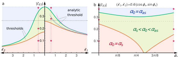
Figure 2: Phase diagram for the nematic director angle $\alpha_{0}$ with respect to the parameters $\left|\tilde{c}_{E3}\right|\propto\left|c_{14}\right|$ and $(\tilde{\kappa}_{1},\tilde{\kappa}_{2})=\tilde{\kappa}_{0}(\cos\phi_{\kappa},\sin\phi_{\kappa})$. In panel (a), the absolute value $\tilde{\kappa}_{0}$ changes for fixed $\phi_{k}=\pi/2$ (left horizontal axis) and $\phi_{k}=0$ (right horizontal axis). In panel (b), the absolute value is fixed at $\tilde{\kappa}_{0}=0.6$ and the relative angle $\phi_{\kappa}\in[0,\pi/2]$ is varied. There are three distinct regimes: (i) For small values of $|c_{E3}|$, and when $\kappa_{1}$ (or $\kappa_{2}$) is much larger than $\kappa_{2}$ (or $\kappa_{1}$), the nematic director is locked at the high-symmetry directions $\alpha_{s}$ (red region). (ii) For large values of $|c_{E3}|$, regardless of $\tilde{\kappa}_{i}$, the nematic director aligns with the “anti-symmetry directions” $\alpha_{as}$ (blue region). (iii) For intermediate values of $|c_{E3}|$, or when $\kappa_{1}$ and $\kappa_{2}$ are comparable, the nematic director evolves smoothly between $\alpha_{s}<\alpha_{0}<\alpha_{as}$ (green region). The full dependence of $\alpha_{0}$ and $\hat{\boldsymbol{q}}_{0}$ on $\left|\tilde{c}_{E3}\right|$, for a given maximum of $R(\hat{\boldsymbol{q}}_{0},\alpha_{0})$, is shown in Fig. 3 for the $(\tilde{\kappa}_{1},\tilde{\kappa}_{2})$ values corresponding to the two red dashed lines. For the six parameter values corresponding to the red stars, the function $R(\hat{\boldsymbol{q}}_{0},\alpha_{0}(\hat{\boldsymbol{q}}_{0}))$ is plotted in Fig. 4. The horizontal black dotted line denotes the expected value of $\tilde{c}_{E3}=-0.265$ for doped $\mathrm{Bi_{2}Se_{3}}$ (Gao et al., 2016). The topmost light-blue horizontal dashed line denotes the limit of structural stability as given by the condition $|c_{E3}|_{\mathrm{max}}=\sqrt{c_{E1}c_{E2}}$, see Eq. (20). The analytical thresholds stem from the calculations presented in Section III.2.4.

III Mean-field analysis of the effective nematic action

We now analyze the full effective action (35) that includes both the pure nematic action $\mathcal{S}_{\mathrm{nem}}$, Eq. (8), and the phonon-induced contribution $\mathcal{S}^{\prime}$, Eq. (46). Because the upper critical dimension of the three-state Potts model is below $3$, see Ref. (Wu, 1982), our model is expected to be well-described by mean-field theory in three dimensions. The mean-field nematic order parameter is given by $\boldsymbol{\Phi}_{q}^{E_{g}}=\delta_{\omega_{n},0}\delta_{q,0}\,|\boldsymbol{\Phi}_{0}^{E_{g}}|(\cos\alpha_{0},\sin\alpha_{0})^{T}$ with homogeneous field values $|\boldsymbol{\Phi}_{0}^{E_{g}}|$ and $\alpha_{0}$. The effective mean-field action $\mathcal{S}_{\mathrm{eff}}=\frac{V}{T}\int_{\hat{\boldsymbol{q}}}\mathcal{S}_{\mathrm{eff},\hat{\boldsymbol{q}}}$ becomes

$$\mathcal{S}_{\mathrm{eff},\hat{\boldsymbol{q}}} =\frac{r\!-\!M(\hat{\boldsymbol{q}},\alpha_{0})}{2}|\boldsymbol{\Phi}_{0}^{E_{g}}|^{2}+\!g|\boldsymbol{\Phi}_{0}^{E_{g}}|^{3}\!\cos(3\alpha_{0})\!+\!u|\boldsymbol{\Phi}_{0}^{E_{g}}|^{4},$$

$$=\frac{1}{2}|\boldsymbol{\Phi}_{0}^{E_{g}}|^{2}\left[r-\tilde{R}(\hat{\boldsymbol{q}},\alpha_{0},|\boldsymbol{\Phi}_{0}^{E_{g}}|)\right],$$ (47)

where we introduced the momentum-dependent nematic mass function

$$M(\hat{\boldsymbol{q}},\alpha_{0}) =\Pi_{(\boldsymbol{q},0)}^{A_{1g}}+\boldsymbol{\Pi}_{(\boldsymbol{q},0)}^{E_{g}}\cdot\left(\!\!\!\begin{array}[]{c}\cos(2\alpha_{0})\\ -\sin(2\alpha_{0})\end{array}\!\!\!\right)\!,$$ (50)

and the auxiliary function

$$\tilde{R}(\hat{\boldsymbol{q}},\alpha_{0},|\boldsymbol{\Phi}_{0}^{E_{g}}|) =M(\hat{\boldsymbol{q}},\alpha_{0})+\frac{g^{2}\cos^{2}(3\alpha_{0})}{2u}$$

$$\quad-\!2u\Big{[}|\boldsymbol{\Phi}_{0}^{E_{g}}|+\frac{g\cos(3\alpha_{0})}{2u}\Big{]}^{2}.$$ (51)

We highlight the key role played by the cubic nematic term in Eq. (47). In a harmonic approximation, where this term is absent, and in the special case where $c_{14}=0$, the nematic director angle $\alpha_{0}$ can assume any value and all in-plane directions in momentum space are equivalent. This is consistent with the fact that the pure transverse acoustic phonon dispersion is in-plane isotropic in this case (Kimura et al., 2021). However, the cubic term is relevant in the renormalization-group sense, and lowers the symmetry of $\boldsymbol{\Phi}^{E_{g}}$ from SO(2) to $Z_{3}$-Potts (Lou et al., 2007). Moreover, in three dimensions, it induces a first-order transition, in which case the cubic term is not necessarily subleading compared to the quadratic term. It is the competition between these two terms that restricts both the nematic director and the soft momentum-space directions. In a phonon description, this cubic term is equivalent to an anharmonic phonon term, which causes the phonon properties to no longer be isotropic in the plane (see, for instance, Ref. (Paulatto et al., 2013)).

The nematic phase transition occurs when $\mathcal{S}_{\mathrm{eff},\hat{\boldsymbol{q}}}=0$, which due to the cubic term happens when $|\boldsymbol{\Phi}_{0}^{E_{g}}|$ jumps to a non-zero value. Thus, the first-order transition temperature can be identified from the maximum of $\tilde{R}(\hat{\boldsymbol{q}},\alpha_{0},|\boldsymbol{\Phi}_{0}^{E_{g}}|)$. Maximizing Eq. (51) leads to the non-zero nematic value at the first-order transition

$$|\boldsymbol{\Phi}_{0}^{E_{g}}| =\frac{|g|}{2u}|\cos(3\alpha_{0})|,$$ (52)

and to the condition

$$\text{sign}\left(g\cos(3\alpha_{0})\right) <0.$$ (53)

Note that the case of a pure nematic order parameter, for which $\alpha_{0}=\{0,2,4\}\frac{\pi}{3}$ for $g<0$ and $\alpha_{0}=\{1,3,5\}\frac{\pi}{3}$ for $g>0$ satisfies this condition. Hence, the last line in (51) vanishes at the maximum, and the auxiliary function that remains to be maximized becomes:

$$R(\hat{\boldsymbol{q}},\alpha_{0}) =M(\hat{\boldsymbol{q}},\alpha_{0})+\frac{g^{2}\cos^{2}(3\alpha_{0})}{2u}.$$ (54)

Importantly, the maximization is with respect to the three variables $\{\hat{\boldsymbol{q}},\alpha_{0}\}$, corresponding to the two independent directions in momentum space and to the nematic director angle $\alpha_{0}$. Hereafter, we denote the momentum direction along which (54) is maximized by $\hat{\boldsymbol{q}}_{0}=(\cos\varphi_{0}\sin\theta_{0},\sin\varphi_{0}\sin\theta_{0},\cos\theta_{0})^{T}$. The nematic transition temperature is given by $T_{\mathrm{nem}}=T_{\mathrm{nem}}^{0}+r^{\mathrm{nem}}/a_{\mathsf{c}}$ with:

$$r^{\mathrm{nem}} =\max_{\hat{\boldsymbol{q}},\alpha_{0}}\left[R(\hat{\boldsymbol{q}},\alpha_{0})\right].$$ (55)

As demonstrated in Appendix C, the maxima of $R(\hat{\boldsymbol{q}},\alpha_{0})$ occur in multiples of $12$. Indeed, if $\{\hat{\boldsymbol{q}}_{0},\alpha_{0}\}$ is a maximum of $R$, symmetry enforces the following relationships:

$$R(-\hat{\boldsymbol{q}}_{0},\alpha_{0}) =R(\hat{\boldsymbol{q}}_{0},\alpha_{0}),$$ (56)

$$R\big{[}\mathcal{R}_{v}^{\pm}(C_{3z})\hat{\boldsymbol{q}}_{0},\alpha_{0}\mp\frac{2\pi}{3}\big{]} =R(\hat{\boldsymbol{q}}_{0},\alpha_{0}),$$ (57)

$$R\big{[}\mathcal{R}_{v}(IC_{2n_{s}})\hat{\boldsymbol{q}}_{0},\alpha_{s}-\delta\big{]} =R(\hat{\boldsymbol{q}}_{0},\alpha_{s}+\delta),$$ (58)

with the definitions of the symmetry elements and transformation matrices provided in the appendix. Importantly, the relationship (58) implies that a finite deviation $\delta\neq 0$ away from a high-symmetry direction $\alpha_{s}$ necessarily induces two maxima $\alpha_{0}=\alpha_{s}\pm\delta$, i.e. the nematic director splits into two, doubling the number of non-identical directors from $3$ to $6$, see Fig. 1. As we show in the following sections, each direction $\alpha_{0}$ is associated with $4$ soft momentum-space directions $\hat{\boldsymbol{q}}_{0}$. This implies that the function $R$ has either $12$ or $24$ degenerate maxima depending on whether $\alpha_{0}=\alpha_{s}$ or $\alpha_{0}\neq\alpha_{s}$, respectively.

[][]

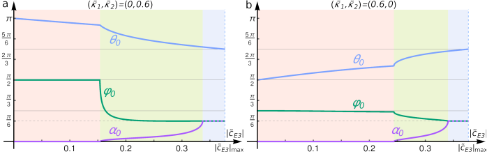
Figure 3: The soft momentum-space direction $\hat{\boldsymbol{q}}_{0}$ (parametrized by the polar angle $\theta_{0}$ and the azimuthal angle $\varphi_{0}$) and the nematic director angle $\alpha_{0}$ associated with a particular maximum of $R(\hat{\boldsymbol{q}}_{0},\alpha_{0})$ are plotted as a function of $\left|\tilde{c}_{E3}\right|$ for the two indicated $(\tilde{\kappa}_{1},\tilde{\kappa}_{2})$ values, which correspond to the red dashed lines in Fig. 2.

III.1 Numerical results

We proceed with a numerical investigation of the maxima of $R(\hat{\boldsymbol{q}},\alpha_{0})$. We consider three independent “tuning” parameters: the two effective nemato-elastic coupling constants $\tilde{\kappa}_{i}=\kappa_{i}\sqrt{u}/g$, with $i=\{1,2\}$, and the dimensionless $\tilde{c}_{E3}=c_{E3}/c_{0}$, with a reference elastic constant $c_{0}=100\,\mathrm{GPa}$. The other elastic constants are set to the values of $\mathrm{Bi_{2}}\mathrm{Se}_{3}$. In Fig. 2, we present the “phase diagram” for the nematic director in this parameter space. Parametrizing the two coupling constants as $(\tilde{\kappa}_{1},\tilde{\kappa}_{2})=\tilde{\kappa}_{0}(\cos\phi_{\kappa},\sin\phi_{\kappa})$, panel (a) shows the phase diagram when $\phi_{k}$ is fixed ($\phi_{k}=\pi/2$ on the left side and $\phi_{k}=0$ on the right side) whereas panel (b) presents the phase diagram for fixed $\tilde{\kappa}_{0}$. We identify three distinct phases: (i) the nematic director aligns with the high-symmetry directions, $\alpha_{0}=\alpha_{s}$ (red region), where $\alpha_{s}\in\{0,2,4\}\frac{\pi}{3}$ or $\alpha_{s}\in\{1,3,5\}\frac{\pi}{3}$; (ii) the nematic director evolves smoothly between the high-symmetry and the “anti-symmetry” directions (green region); (iii) the nematic director aligns with one of the “anti-symmetry” directions, $\alpha_{0}=\alpha_{as}$ (blue region), where $\alpha_{as}\in\{1,3,5,7,9,11\}\frac{\pi}{6}$. We conclude that for the nematic director to unlock from the high-symmetry directions, it requires a threshold value for $c_{E3}$ or the simultaneous presence of both $\tilde{\kappa}_{1}$ and $\tilde{\kappa}_{2}$. The horizontal black dotted line in both panels of Fig. 2 marks the value of $c_{E3}$ expected for $\mathrm{Bi_{2}Se_{3}}$. Therefore, regardless of the values of the coupling constants, the nematic director in doped $\mathrm{Bi_{2}Se_{3}}$ is expected to be unlocked from the high-symmetry directions. The light-blue dashed horizontal line (the top line) denotes the limit of structural stability, defined by $|c_{E3}|_{\mathrm{max}}=\sqrt{c_{E1}c_{E2}}$ [or $\mathsf{d}_{E}=0$, see Eq. (20)]. For this value of $c_{E3}$, the system would undergo a structural transition on its own, even without the coupling to nematic degrees of freedom. Upon approaching this boundary, the system tends to align the nematic director with the “anti-symmetry” directions.

The two vertical red dotted lines in Fig. 2 mark the $(\tilde{\kappa}_{1},\tilde{\kappa}_{2})$-values for which the complete $\alpha_{0}$ and $\hat{\boldsymbol{q}}_{0}=(\cos\varphi_{0}\sin\theta_{0},\sin\varphi_{0}\sin\theta_{0},\cos\theta_{0})^{T}$ evolutions as a function of $c_{E3}$ are shown in Fig. 3. Additionally, for the six $c_{E3}$ values indicated by the red stars, we present in Fig. 4 the $R(\hat{\boldsymbol{q}},\alpha_{0}(\hat{\boldsymbol{q}}))$ dependence on $\varphi$ and $\theta$. In all panels, there are clear maxima at well-defined $\left(\varphi_{0},\theta_{0}\right)$ points; the corresponding value for the nematic director angle $\alpha_{0}(\hat{\boldsymbol{q}}_{0})$ at these maxima is indicated in the figure. For clarity, we only show the nematic director $\alpha_{0}(\hat{\boldsymbol{q}})$ that falls within the interval $\alpha_{0}\in[-\frac{\pi}{3},\frac{\pi}{3}]$. The other symmetry-equivalent nematic directors can be obtained in a straightforward way from Eqs. (56)-(58). Panels (a) and (d) of Fig. 4 show the case in which the nematic director is locked at the high-symmetry directions $\alpha_{0}=\alpha_{s}$ (red region in the phase diagram of Fig. 2(a)). Each nematic director is associated with four distinct “soft” momentum directions $\left(\varphi_{0},\theta_{0}\right)$, two of which are in the interval $\varphi\in[0,\pi)$ (shown in the figure) and two of which are in the interval $\varphi\in[\pi,2\pi)$ (not shown in the figure). Panels (b) and (e) show the behavior of $R(\hat{\boldsymbol{q}},\alpha_{0}(\hat{\boldsymbol{q}}))$ in the green region of the phase diagram of Fig. 2(a), for which $\alpha_{s}<\alpha_{0}<\alpha_{as}$. We note that the number of maxima of $R(\hat{\boldsymbol{q}},\alpha_{0}(\hat{\boldsymbol{q}}))$ doubles as soon as the nematic director unlocks from $\alpha_{s}$. Even in this case, it still holds that every nematic director angle is associated with four soft directions $\hat{\boldsymbol{q}}_{0}$ in momentum space. In panels (c) and (f), we show how the function $R(\hat{\boldsymbol{q}},\alpha_{0}(\hat{\boldsymbol{q}}))$ looks like in the blue region of the phase diagram in Fig. 2(a), corresponding to $\alpha_{0}=\alpha_{as}$. In this case, the soft directions in momentum-space approach the value dictated by the structural instability, see section III.2.2. Note that the light-shaded regions in figures 4(c) and (f) far away from the maxima are an artifact of restricting $\alpha_{0}\in[-\frac{\pi}{3},\frac{\pi}{3}]$.

[][]

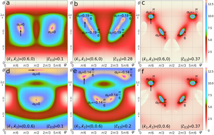
Figure 4: The function $R(\hat{\boldsymbol{q}},\alpha_{0}(\hat{\boldsymbol{q}}))$ is plotted as a function of the momentum-space polar angle $\theta$ and azimuthal angle $\varphi$. Because of the relationship in Eq. (56), we consider only the ranges $\varphi\in[0,\pi)$ and $\theta\in[0,\pi]$. The extremal director angle value $\alpha_{0}(\hat{\boldsymbol{q}})\in[-\frac{\pi}{3},\frac{\pi}{3}]$ is shown at every maxima; note that the other nematic director angles outside of this interval can be obtained from Eq. (57). The value of $\left|\tilde{c}_{E3}\right|$ increases upon moving from the left to the right panels, encompassing the three regions of the phase diagram of Fig. 2(a), as indicated by the red stars. The top (bottom) panels correspond to a non-zero $\kappa_{1}$ ($\kappa_{2}$). The black arrows indicate the maxima previously presented in Fig. 3.

III.2 Analytical approach

To gain further insight into the numerical results, we perform analytical approximations to study the maxima of the function $R(\hat{\boldsymbol{q}},\alpha_{0})$ defined in Eq. (54). We start by rewriting the momentum-dependent mass function (50) as

$$M(\hat{\boldsymbol{q}},\alpha_{0}) =\sum_{j=1}^{3}\frac{\sin^{2}\vartheta_{\hat{\boldsymbol{q}}}^{(j)}}{\tilde{\omega}_{j,\hat{\boldsymbol{q}}}^{2}}\Bigg{\{}\!\kappa_{1}\cos\!\big{(}\alpha_{0}\!+\!\varphi\!+\!\phi_{\hat{\boldsymbol{q}}}^{(j)}\big{)}$$

$$\!\!\!\!\!\!\!\!\!\!\!\!\!\!\!\!\!\!-\kappa_{2}\!\left[\cot\!\vartheta_{\hat{\boldsymbol{q}}}^{(j)}\sin\!\big{(}\alpha_{0}\!-\!\varphi\big{)}\!+\!\cot\!\theta\sin\!\big{(}\alpha_{0}\!-\!\phi_{\hat{\boldsymbol{q}}}^{(j)}\big{)}\!\right]\!\!\!\Bigg{\}}^{\!\!2}\!,$$ (59)

with $\tilde{\omega}_{j,\hat{\boldsymbol{q}}}\equiv\omega_{j,\hat{\boldsymbol{q}}}/\sin\theta$ and the eigenvector and momentum parametrizations

$$\hat{\boldsymbol{e}}_{\boldsymbol{q}}^{(j)} =\left(\cos\phi_{\hat{\boldsymbol{q}}}^{(j)}\sin\vartheta_{\hat{\boldsymbol{q}}}^{(j)},\sin\phi_{\hat{\boldsymbol{q}}}^{(j)}\sin\vartheta_{\hat{\boldsymbol{q}}}^{(j)},\cos\vartheta_{\hat{\boldsymbol{q}}}^{(j)}\right)^{T}\!\!,$$ (60)

$$\hat{\boldsymbol{q}} =\left(\cos\varphi\sin\theta,\sin\varphi\sin\theta,\cos\theta\right)^{T}.$$ (61)

While the analytical expressions for $\omega_{j,\hat{\boldsymbol{q}}}$ and $\hat{\boldsymbol{e}}_{\boldsymbol{q}}^{(j)}$ in terms of the elastic constants are given in Appendix B, we note that the eigenvalues depend on the momentum direction ($\varphi,\theta$) only through three distinct combinations that involve the elastic constant $c_{E3}=c_{14}$:

$$\tilde{\omega}_{j,\hat{\boldsymbol{q}}} =f\left(\cot^{2}\theta,c_{E3}\cot\theta\sin(3\varphi),c_{E3}^{2}\cos(6\varphi)\right).$$

Therefore, in what follows, we consider three different asymptotic limits of $c_{E3}$ that allow us to find simplified analytical expressions for the eigenvalues and eigenvectors of the dynamic matrix and, consequently, for the functions $M(\hat{\boldsymbol{q}},\alpha_{0})$ and $R(\hat{\boldsymbol{q}},\alpha_{0})$. Before delving into these calculations, it is instructive to consider the two different types of strain fluctuations that contribute to the effective mass (59).

III.2.1 Contributions from static and dynamic fluctuations

The elastic fluctuations $\epsilon_{ij}\left(\mathbf{q}\right)$ present in the system can be thought of as arising from two distinct contributions (see also Ref. (Paul and Garst, 2017)): one corresponding to uniform and static strain fluctuations, $\epsilon_{ij}\left(\mathbf{q}=0\right)$, and the other corresponding to dynamic fluctuations, $\epsilon_{ij}\left(\mathbf{q}\neq 0\right)$. The first one gives simply a trivial shift in the mass term, which is the same for all momentum-space directions. The second one is responsible for generating the non-trivial directional dependence of the mass term. Upon performing the partition function integration in Eq. (22) in terms of the lattice displacement fields $D\boldsymbol{u}$, both contributions are accounted for. To see this, and to disentangle these two contributions, it is convenient to consider the hypothetical limit in which only uniform and static strain fluctuations are allowed, which corresponds to computing the partition function integration only over the homogeneous strain field $D\boldsymbol{\epsilon}^{D_{3d}}$. Then, the integration over the static limit of the action (10) with the nemato-elastic coupling (21) leads to the following uniform renormalization of the nematic action:

$$\mathcal{S}_{\mathrm{stat}} =-\frac{1}{2}\frac{V}{T}M_{\mathrm{stat}}|\boldsymbol{\Phi}_{0}^{E_{g}}|^{2},$$ (62)

with the static mass

$$M_{\mathrm{stat}} =\frac{c_{E2}\kappa_{1}^{2}+c_{E1}\kappa_{2}^{2}-2c_{E3}\kappa_{1}\kappa_{2}}{\mathsf{d}_{E}}.$$ (63)

As expected, the mass renormalization is larger the closer the system is to a pure structural transition, corresponding to $\mathsf{d}_{E}\rightarrow 0$. The key point is that the static mass (63) corresponds to the maximum value that the renormalized mass $M(\hat{\boldsymbol{q}},\alpha_{0})$ can possibly attain – which only happens for specific momentum directions $\hat{\boldsymbol{q}}_{0}$ and nematic director angles $\alpha_{0}$. In more mathematical terms, the quadratic part of the effective action (47) can be rewritten as

$$\mathcal{S}_{\mathrm{eff},\hat{\boldsymbol{q}}}^{(2)} =\frac{1}{2}\big{[}r\!-M_{\mathrm{stat}}+\!\delta M(\hat{\boldsymbol{q}},\alpha_{0})\big{]}|\boldsymbol{\Phi}_{0}^{E_{g}}|^{2},$$ (64)

where $\delta M(\hat{\boldsymbol{q}},\alpha_{0})\equiv M_{\mathrm{stat}}-M(\hat{\boldsymbol{q}},\alpha_{0})\geq 0$ denotes the energy cost associated with the angle arrangements, and $\delta M(\hat{\boldsymbol{q}},\alpha_{0})=0$ can only be attained for specific directions. Since a rigorous analytic deduction of these directions is not feasible (except for the special case of $c_{E3}=0$ that we study below), we present the numerically evaluated ratio $M(\hat{\boldsymbol{q}},\alpha_{0})/M_{\mathrm{stat}}$ in momentum space in Fig. 5 where we have inserted the maximum angle $\alpha_{0}$ following from Eq. (50):

$$\tan(2\alpha_{0}) =-\Pi_{(\boldsymbol{q},0)}^{E_{g},2}/\Pi_{(\boldsymbol{q},0)}^{E_{g},1}.$$ (65)

As shown in Fig. 5, there are twelve distinct momentum directions for which $M(\hat{\boldsymbol{q}},\alpha_{0})$ acquires its maximum value, which is equal to $M_{\mathrm{stat}}$. We verified that the qualitative features of $M(\hat{\boldsymbol{q}},\alpha_{0})$ do not depend on the choices of $\left|\tilde{c}_{E3}\right|$, $\kappa_{1}$, and $\kappa_{2}$. Having identified all these maxima to be located at integer multiples of $\pi/6$ with respect to the azimuthal angle $\varphi$, we can analytically determine the twelve directions. We denote the six in-plane directions as $\hat{\boldsymbol{q}}_{1}$ and the six out-of-plane directions as $\hat{\boldsymbol{q}}_{2}$ which are defined through

[][]

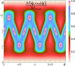
Figure 5: The renormalized mass (59) as a function of the momentum directions $\hat{\boldsymbol{q}}=\hat{\boldsymbol{q}}(\varphi,\theta)$ with the respective maximized director angle $\alpha_{0}(\hat{\boldsymbol{q}})$ inserted according to Eq. (65). The renormalized mass attains its maximum value $M[\hat{\boldsymbol{q}},\alpha_{0}(\hat{\boldsymbol{q}})]=M_{\mathrm{stat}}$ for the twelve directions $\hat{\boldsymbol{q}}_{1,2}$, see Eqs. (66)-(67), indicated by the black dots. The displayed features do not depend on the chosen parameters; for this plot, we set $(\tilde{\kappa}_{1},\tilde{\kappa}_{2})=(2.7,0.9)$ and used the elastic constant values for $\mathrm{Bi_{2}Se_{3}}$. The static mass $M_{\mathrm{stat}}$ is defined in Eq. (63).

$$\hat{\boldsymbol{q}}_{1} : \varphi_{1} =\!\frac{\pi}{6}n_{1}, \cot\theta_{1} =0,$$ (66)

$$\hat{\boldsymbol{q}}_{2} : \varphi_{2} =\!\frac{\pi}{6}n_{2}, \cot\theta_{2} =(\text{-}1)^{\frac{n_{2}+\!1}{2}}\frac{c_{E1}\kappa_{2}\!-\!c_{E3}\kappa_{1}}{c_{E2}\kappa_{1}\!-\!c_{E3}\kappa_{2}},$$ (67)

with $n_{1}\in\{0,2,4,6,8,10\}$ and $n_{2}\in\{1,3,5,7,9,11\}$. In the following, we demonstrate that along these momentum-directions—and for the appropriately chosen director angle—the renormalized mass indeed attains its maximum value $M_{\mathrm{stat}}$.

For the in-plane directions $\hat{\boldsymbol{q}}_{1}$, the eigenvalues $\tilde{\omega}_{j,\hat{\boldsymbol{q}}}\equiv\omega_{j,\hat{\boldsymbol{q}}}/\sin\theta$ simplify to

$$\tilde{\omega}_{1,\boldsymbol{q}_{1}}^{2} =c_{A1}\!+\!c_{E1},$$ (68)

$$\tilde{\omega}_{2,\boldsymbol{q}_{1}}^{2} =\frac{c_{E1}\!+\!c_{E2}}{2}\left[1\!-\!\sqrt{1\!-\!4\mathsf{d}_{E}/(c_{E1}\!+\!c_{E2})^{2}}\,\right],$$ (69)

$$\tilde{\omega}_{3,\boldsymbol{q}_{1}}^{2} =\frac{c_{E1}\!+\!c_{E2}}{2}\left[1\!+\!\sqrt{1\!-\!4\mathsf{d}_{E}/(c_{E1}\!+\!c_{E2})^{2}}\,\right],$$ (70)

whereas the eigenvectors (60) are parametrized by:

$$\phi_{\hat{\boldsymbol{q}}_{1}}^{(1)}\! =\varphi_{1}, \sin\vartheta_{\hat{\boldsymbol{q}}_{1}}^{(1)}\! =1, \cos\vartheta_{\hat{\boldsymbol{q}}_{1}}^{(1)}\! =0,$$

$$\phi_{\hat{\boldsymbol{q}}_{1}}^{(2)}\! =\pi\!+\!\frac{\pi}{2}\!\frac{c_{E3}}{|c_{E3}|}\!-\!2\varphi_{1}, \sin\vartheta_{\hat{\boldsymbol{q}}_{1}}^{(2)}\! =\gamma^{-}, \cos\vartheta_{\hat{\boldsymbol{q}}_{1}}^{(2)}\! =\gamma^{+},$$

$$\phi_{\hat{\boldsymbol{q}}_{1}}^{(3)}\! =\pi\!-\!\frac{\pi}{2}\!\frac{c_{E3}}{|c_{E3}|}\!-\!2\varphi_{1}, \sin\vartheta_{\hat{\boldsymbol{q}}_{1}}^{(3)}\! =\gamma^{+}, \cos\vartheta_{\hat{\boldsymbol{q}}_{1}}^{(3)}\! =\gamma^{-}.$$ (71)

In these expressions, we defined:

$$\gamma^{\pm} =\frac{1}{\sqrt{2}}\Big{(}1\pm\frac{c_{E1}\!-\!c_{E2}}{\sqrt{\big{(}c_{E1}\!+\!c_{E2}\big{)}^{2}\!-\!4\mathsf{d}_{E}}}\Big{)}^{\frac{1}{2}}.$$

The insertion into the renormalized mass (59) leads to

$$M(\hat{\boldsymbol{q}}_{1},\alpha_{0})= M_{1}\cos^{2}\left(\alpha_{0}\!+\!\frac{\pi}{3}n_{1}\right)+M_{\mathrm{stat}}\sin^{2}\left(\alpha_{0}\!+\!\frac{\pi}{3}n_{1}\right),$$ (72)

with $M_{1}=\kappa_{1}^{2}/(c_{A1}\!+\!c_{E1})<M_{\mathrm{stat}}$, see App. D.

Before we further analyze Eq. (72), we derive a similar expression for the out-of-plane directions $\hat{\boldsymbol{q}}_{2}$. To do this, we introduce the direction $\hat{\boldsymbol{q}}_{\bar{2}}=\hat{\boldsymbol{q}}_{\bar{2}}[\varphi_{2},\theta]$ which shares the same azimuthal angle with $\hat{\boldsymbol{q}}_{2}$ but keeps $\theta$ arbitrary, such that $\hat{\boldsymbol{q}}_{2}=\hat{\boldsymbol{q}}_{\bar{2}}[\varphi_{2},\theta_{2}]$. For the directions $\hat{\boldsymbol{q}}_{\bar{2}}$ the eigensystem can be derived as

$$\tilde{\omega}_{1,\hat{\boldsymbol{q}}_{\bar{2}}}^{2} =c_{E2}\!+\!c_{A2}\cot^{2}\!\theta+\frac{1}{2}\lambda_{1,\theta}+\!\frac{1}{2}\lambda_{0,\theta},$$ (73)

$$\tilde{\omega}_{2,\hat{\boldsymbol{q}}_{\bar{2}}}^{2} =c_{E1}+2c_{E3}(\text{-}1)^{\frac{n_{2}+1}{2}}\cot\theta+c_{E2}\cot^{2}\theta$$ (74)

$$\tilde{\omega}_{3,\hat{\boldsymbol{q}}_{\bar{2}}}^{2} =c_{E2}\!+\!c_{A2}\cot^{2}\!\theta+\frac{1}{2}\lambda_{1,\theta}-\!\frac{1}{2}\lambda_{0,\theta}\!,$$ (75)

with

$$\phi_{\hat{\boldsymbol{q}}_{\bar{2}}}^{(1)}\! =\!\varphi_{2}\!+\!\frac{\pi}{2}\!-\!\frac{\pi}{2}\!\frac{\lambda_{2,\theta}}{|\lambda_{2,\theta}|}, \sin\vartheta_{\hat{\boldsymbol{q}}_{\bar{2}}}^{(1)}\! =\!\beta_{\theta}^{+}, \cos\vartheta_{\hat{\boldsymbol{q}}_{\bar{2}}}^{(1)}\! =\!\beta_{\theta}^{-},$$

$$\phi_{\hat{\boldsymbol{q}}_{\bar{2}}}^{(2)}\! =\!\varphi_{2}-\frac{\pi}{2}, \sin\vartheta_{\hat{\boldsymbol{q}}_{\bar{2}}}^{(2)}\! =\!1, \cos\vartheta_{\hat{\boldsymbol{q}}_{\bar{2}}}^{(2)}\! =\!0,$$

$$\phi_{\hat{\boldsymbol{q}}_{\bar{2}}}^{(3)}\! =\!\varphi_{2}\!+\!\frac{3\pi}{2}\!-\!\frac{\pi}{2}\!\frac{\lambda_{2,\theta}}{|\lambda_{2,\theta}|}, \sin\vartheta_{\hat{\boldsymbol{q}}_{\bar{2}}}^{(3)}\! =\!\beta_{\theta}^{-}, \cos\vartheta_{\hat{\boldsymbol{q}}_{\bar{2}}}^{(3)}\! =\!\beta_{\theta}^{+},$$ (76)

and the following auxiliary functions:

$$\lambda_{0,\theta} =\sqrt{\lambda_{1,\theta}^{2}+\lambda_{2,\theta}^{2}},$$ (77)

$$\lambda_{1,\theta} =c_{A1}\!+\!c_{E1}\!-\!c_{E2}\!-\!2c_{E3}(\text{-}1)^{\frac{n_{2}+1}{2}}\cot\!\theta\!$$

$$\quad+\!(c_{E2}\!-\!c_{A2})\cot^{2}\!\theta,$$ (78)

$$\lambda_{2,\theta} =2(c_{A3}+c_{E2})\cot\theta-2c_{E3}(\text{-}1)^{\frac{n_{2}+1}{2}},$$ (79)

$$\beta_{\theta}^{\pm} =\frac{1}{\sqrt{2}}\sqrt{1\pm\frac{\lambda_{1,\theta}}{\lambda_{0,\theta}}}\,.$$ (80)

Again, we insert these expressions into the renormalized mass (59) to find

[][]

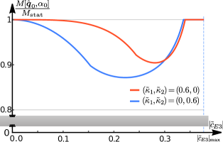
Figure 6: The ratio of the renormalized mass (59) and the static mass (63) as a function of $c_{E3}$ for the two maxima of the function $R(\hat{\boldsymbol{q}},\alpha_{0})$ presented in Fig. 3. The renormalized mass is maximum, i.e. $M[\hat{\boldsymbol{q}}_{0},\alpha_{0}]=M_{\mathrm{stat}}$, for $c_{E3}=0$, and above the upper threshold value beyond which the acoustic phonon contribution is dominant over the anharmonic contribution.

$$M(\hat{\boldsymbol{q}}_{\bar{2}},\alpha_{0})= M_{\theta}^{c}\cos^{2}\left(\alpha_{0}\!+\!\frac{\pi}{3}n_{1}\right)+M_{\theta}^{s}\sin^{2}\left(\alpha_{0}\!+\!\frac{\pi}{3}n_{1}\right),$$ (81)

with $M_{\theta}^{s}$, and $M_{\theta}^{c}$ defined in Appendix D. The maximum amplitude of Eq. (81) is $M_{\mathrm{stat}}$ and it is reached at the polar angle $\theta_{2}$ [Eq. (67)] for which it holds $M_{\theta_{2}}^{s}=M_{\mathrm{stat}}$.

Having derived the renormalized mass expressions for the twelve momentum-directions, $M(\hat{\boldsymbol{q}}_{1},\alpha_{0})$ in Eq. (72) and $M(\hat{\boldsymbol{q}}_{2},\alpha_{0})=M(\hat{\boldsymbol{q}}_{\bar{2}}[\varphi_{2},\theta_{2}],\alpha_{0})$ in Eq. (81), it is straight-forward to identify the corresponding nematic director angles $\alpha_{0}$ for which $M(\hat{\boldsymbol{q}}_{1,2},\alpha_{0})=M_{\mathrm{stat}}$. In both cases, the condition becomes

$$\alpha_{0}\!+\!\frac{\pi}{3}n_{1,2} =\frac{\pi}{2}\{\pm 1,\pm 3,\dots\}.$$ (82)

Equation (82) is only satisfied for director angles that align with the “anti-symmetry” directions $\alpha_{0}=\alpha_{as}\in\frac{\pi}{6}\{1,3,5,7,9,11\}$. Each of these nematic directors $\alpha_{0}=\alpha_{as}$ entails four soft directions in momentum space, two within the $\hat{\boldsymbol{q}}_{1}$ manifold and two within the $\hat{\boldsymbol{q}}_{2}$ manifold. For example, for $\alpha_{0}=\frac{\pi}{6}$, the four momentum directions that maximize the renormalized mass are parametrized by $n_{1}=\{4,10\}$ and $n_{2}=\{1,7\}$.

This analysis provides an interesting insight about the two contributions to the mass term $M(\hat{\boldsymbol{q}},\alpha_{0})$. While the uniform and static strain fluctuations enhance the tendency towards nematic order for all momentum directions ($M_{\mathrm{stat}}$), the dynamic fluctuations penalizes those directions that do not conform to the constraints imposed by the anisotropy of the phonon dispersions – i.e. those for which $\delta M(\hat{\boldsymbol{q}},\alpha_{0})>0$. As a result, only certain momentum directions become soft at the transition.

It is important to note that the total function $R(\hat{\boldsymbol{q}},\alpha_{0})$ in Eq. (54), which needs to be maximized to give the leading instability, also contains—besides the mass term $M(\hat{\boldsymbol{q}},\alpha_{0})$—the anharmonic contribution $\cos^{2}(3\alpha_{0})$:

$$R(\hat{\boldsymbol{q}},\alpha_{0})=M(\hat{\boldsymbol{q}},\alpha_{0})+\frac{g^{2}\cos^{2}(3\alpha_{0})}{2u}.$$ (83)

The last term favors the nematic director to align with the high-symmetry directions $\alpha_{s}\in\{0,1,2,3,4,5\}\frac{\pi}{3}$. It is the competition between these two terms that gives rise to the rich phase diagram obtained numerically in Fig. 2. Indeed, as shown in Fig. 6, the mass term $M(\hat{\boldsymbol{q}},\alpha_{0})$ computed at the maximum of $R(\hat{\boldsymbol{q}},\alpha_{0})$ can not overcome $M_{\mathrm{stat}}$. It reaches equality in the hexagonal limit where $|c_{E3}|=0$, and above the upper threshold value when the system approaches the pure structural phase transition $|c_{E3}|\rightarrow\sqrt{c_{E1}c_{E2}}$. In the remainder of this section, we analyze these two regimes asymptotically, as well as the intermediate regime perturbatively.

III.2.2 Limit $|c_{E3}|_{\mathrm{max}}=\sqrt{c_{E1}c_{E2}}$

In the limit $|c_{E3}|_{\mathrm{max}}=\sqrt{c_{E1}c_{E2}}$, corresponding to $\mathsf{d}_{E}=c_{E1}c_{E2}-c_{E3}^{2}=0$, the elastic action (10) becomes unstable, see Eq. (20). In other words, one of the sound velocities $\omega_{j,\hat{\boldsymbol{q}}}$ of the dynamic matrix vanishes, and the system undergoes a pure structural phase transition. In this limit, corresponding to the vicinity of the top dashed light-blue line in figure 2, the renormalized mass term (59) diverges along certain directions. These soft momentum directions are, of course, the $12$ directions $\hat{\boldsymbol{q}}_{1}$ and $\hat{\boldsymbol{q}}_{2}$ defined in Sec. III.2.1 along which the renormalized mass attains its maximum value $M_{\mathrm{stat}}$. The phonon mode that becomes soft corresponds to the eigenvalue $\omega_{2,\hat{\boldsymbol{q}}_{1}}$ in Eq. (69) and $\omega_{2,\hat{\boldsymbol{q}}_{2}}$ in Eq. (74). Indeed, in the limit $\mathsf{d}_{E}\rightarrow 0$, they simplify to:

$$\tilde{\omega}_{2,\boldsymbol{q}_{1}}^{2} \approx\frac{1}{c_{E1}\!+\!c_{E2}}\mathsf{d}_{E},$$ (84)

$$\tilde{\omega}_{2,\hat{\boldsymbol{q}}_{2}}^{2} =\frac{c_{E2}\kappa_{1}^{2}+c_{E1}\kappa_{2}^{2}-2c_{E3}\kappa_{1}\kappa_{2}}{\left(c_{E2}\kappa_{1}-c_{E3}\kappa_{2}\right)^{2}}\mathsf{d}_{E}.$$ (85)

Because $M_{\mathrm{stat}}\sim 1/\mathsf{d}_{E}$, the mass-term contribution to $R(\hat{\boldsymbol{q}},\alpha_{0})$ is much larger than the anharmonic contribution, which has coefficient $g^{2}/2u$. As a result, the maxima of $R(\hat{\boldsymbol{q}},\alpha_{0})$ coincide with the maxima of $M(\hat{\boldsymbol{q}},\alpha_{0})$ in the regime where $\mathsf{d}_{E}\rightarrow 0$. Hence, according to the condition (82), the nematic director angle aligns with the “anti-symmetry” directions $\alpha_{0}=\alpha_{as}\in\frac{\pi}{6}\{1,3,5,7,9,11\}$, in agreement with the findings depicted in Fig. 4(c,f). Interestingly, for the elastic constants values reported for $\mathrm{Bi_{2}Se_{3}}$, the soft polar angle (67) approaches

$$\cot\theta_{2} \rightarrow\pm\sqrt{\frac{c_{E1}}{c_{E2}}}=\pm\sqrt{\frac{753}{754}}\approx\pm 1,$$

at the pure structural instability. Therefore, the soft polar angle is very close to $\theta_{2}\approx\{\pi/4,\,3\pi/4\}$, as can be seen in Fig. 4(c,f) or Fig. 3.

It is important to note that when $\alpha_{0}=\alpha_{as}$, the cubic term of the action (47) vanishes and the nematic transition becomes second-order—at least within our mean-field approximation. This is reflected in our formalism by the fact that the jump of the nematic order parameter in Eq. (52) vanishes when $\alpha_{0}=\alpha_{as}$. Consequently, the condition (53) does not need to be satisfied in this case.

III.2.3 Limit $c_{E3}=0$

In this limit, the elastic properties become the same as that of a hexagonal lattice. The eigenvalues and eigenvectors are given by Eqs. (73)-(80) with $c_{E3}=0$ and $\varphi_{2}\rightarrow\varphi$. Inserting these expressions into the renormalized mass (59) gives:

$$M(\hat{\boldsymbol{q}},\alpha_{0}) =\kappa_{1}^{2}A_{\theta}^{-}\cos(2\alpha_{0}+\!4\varphi)\!+\!\kappa_{2}^{2}B_{\theta}^{-}\cos(2\alpha_{0}-\!2\varphi)$$

$$\!\!\!\!\!\!\!\!\!\!\!\!\!\!\!\!\!+\!\kappa_{1}^{2}A_{\theta}^{+}\!+\!\kappa_{2}^{2}B_{\theta}^{+}\!-\!2\kappa_{1}\kappa_{2}\!\left(C_{\theta}^{+}\!\sin(2\alpha_{0}+\varphi)\!-\!C_{\theta}^{-}\!\sin(3\varphi)\right)\!.$$ (86)

The functions $A_{\theta}^{\pm}$, $B_{\theta}^{\pm}$ and $C_{\theta}^{\pm}$ depend only on the polar angle $\theta$, and are given explicitly in Appendix D. Now, in the limit $c_{E3}=0$, for consistency one must also impose $\kappa_{2}=0$, since the symmetry that enforces a vanishing $c_{E3}$ also makes the out-of-plane and in-plane shear strain doublets in Eq. (17) belong to different irreducible representations. Then, the function $R(\hat{\boldsymbol{q}},\alpha_{0})$ in Eq. (51) becomes

$$R(\hat{\boldsymbol{q}},\alpha_{0}) =\kappa_{1}^{2}A_{\theta}^{+}+\kappa_{1}^{2}A_{\theta}^{-}\cos(2\alpha_{0}\!+\!4\varphi)+\frac{g^{2}\cos^{2}(3\alpha_{0})}{2u}.$$ (87)

As demonstrated in Appendix D, the function (87) is maximized with respect to $\theta$ at $\theta_{0}=\pi/2$, leading to

$$R(\varphi,\theta_{0},\alpha_{0}) =\kappa_{1}^{2}\frac{c_{E1}\!+\!c_{A1}\sin^{2}(\alpha_{0}\!+\!2\varphi)}{\left(c_{A1}\!+\!c_{E1}\right)c_{E1}}\!+\!\frac{g^{2}\cos^{2}(3\alpha_{0})}{2u}.$$ (88)

Note that the first term in the expression (88) is the mass term, whose maximum is given by $\kappa_{1}^{2}/c_{E1}$. This agrees with the expression for $M_{\mathrm{stat}}$ [Eq. (63)] in the limit $\kappa_{2}=0$, $c_{E3}=0$. Moreover, in contrast to the case where $c_{E3}\neq 0$, the values of $\varphi$ that maximize the mass term are not restricted to the discrete values given by Eqs. (66) and (67). On the contrary, maximization of the mass term alone only restricts the combination $\alpha_{0}+2\varphi=\frac{\pi}{2}n$, with $n=\{1,3,5,7\}$. This is also related to the fact that $\theta_{2}=\theta_{1}=\pi/2$ in Eq. (67).

Because of this peculiarity of the $c_{E3}=0$ term, the two terms that contribute to $R(\varphi,\theta_{0},\alpha_{0})$ in Eq. (88) can be simultaneously maximized with respect to $\varphi$ and $\alpha_{0}$. We obtain:

$$\alpha_{0} =\alpha_{s}, \varphi =\frac{\pi}{4}n-\frac{1}{2}\alpha_{0}.$$ (89)

Thus, the nematic director aligns with the high-symmetry directions, and it is associated with the four momentum directions that correspond to $n=\{1,3,5,7\}$. This result is in agreement with the findings of Ref. (Fernandes and Venderbos, 2020), where the case of the $\mathsf{D_{6}}$ point group was considered.

III.2.4 Expansion in $|c_{E3}|$

The fact that the two limiting cases $c_{E3}=0$ and $|c_{E3}|=\sqrt{c_{E1}c_{E2}}$ favor $\alpha_{0}=\alpha_{s}$ and $\alpha_{0}=\alpha_{as}$, respectively, suggests that the nematic director has to rotate as $|c_{E3}|$ is increased. We thus expand the renormalized mass in powers of small $|c_{E3}|$ to elucidate how the rotation actually occurs. Formally, we have:

$$M(\hat{\boldsymbol{q}},\alpha_{0}) =\!\kappa_{1}^{2}\Big{(}\!M_{\hat{\boldsymbol{q}},\alpha_{0}}^{(0)}\!+\!M_{\hat{\boldsymbol{q}},\alpha_{0}}^{(2)}c_{E3}^{2}\!+\!M_{\hat{\boldsymbol{q}},\alpha_{0}}^{(4)}c_{E3}^{4}+\dots\Big{)}.$$ (90)

To keep the analysis transparent, we set $\kappa_{2}=0$. Additionally, we expand the momentum directions according to

$$\varphi =\varphi^{(0)}+\varphi^{(1)}c_{E3}+\varphi^{(2)}c_{E3}^{2}+\varphi^{(3)}c_{E3}^{3}+\dots,$$ (91)

$$\cot\theta =\Theta^{(0)}+\Theta^{(1)}c_{E3}+\Theta^{(2)}c_{E3}^{2}+\Theta^{(3)}c_{E3}^{3}+\dots.$$ (92)

We are now in position to maximize the renormalized mass order by order in $c_{E3}$.

The zeroth order contribution to $M_{\hat{\boldsymbol{q}},\alpha_{0}}$ is given by Eq. (86) with $A_{\theta}^{\pm}$ defined in Appendix D. Also shown in the Appendix D is the analysis to determine the corresponding maxima at

$$\Theta^{(0)} =0, \varphi^{(0)} =\frac{\pi}{4}N_{0}-\frac{1}{2}\alpha_{0},$$ (93)

with $N_{0}=\{1,3,5,7\}$. This recovers the result that, for $c_{E3}=0$, the maxima reside on the equator, $\theta=\pi/2$ [see Fig. 3(b)]. Then, the zeroth order contribution to the mass becomes

$$M_{\hat{\boldsymbol{q}},\alpha_{0}}^{(0)} =\frac{1}{c_{E1}},$$ (94)

which is independent of $\alpha_{0}$.

To second order, the renormalized mass is given by

$$M_{\hat{\boldsymbol{q}},\alpha_{0}}^{(2)} =\frac{-4c_{A1}\left(\varphi^{(1)}\right)^{2}}{\left(c_{A1}\!+\!c_{E1}\right)c_{E1}}-\frac{c_{E2}}{c_{E1}^{2}}\!\left(\!\Theta^{(1)}\!-\!\Theta_{0}^{(1)}\!\right)^{2}\!\!+\!\frac{1}{c_{E2}c_{E1}^{2}},$$ (95)

which is maximized by

$$\varphi^{(1)} \!=\!0, \Theta^{(1)} \!=\Theta_{0}^{(1)}\!=\!\frac{1}{c_{E2}}\sin\!\Big{(}\frac{3\pi}{4}N_{0}-\frac{3\alpha_{0}}{2}\!\Big{)}.$$ (96)

Because Eq. (95) remains independent of the nematic director angle $\alpha_{0}$, the latter is still determined solely by the contribution arising from the bare nematic action, namely, the $\cos^{2}(3\alpha_{0})$ term in Eq. (54), which favors $\alpha_{0}=\alpha_{s}$. Therefore, to describe the unlocking of the nematic director from the high-symmetry directions, it is necessary to go to higher-order in $c_{E3}$.

The fourth-order contribution to the renormalized mass is given by:

$$M_{\hat{\boldsymbol{q}},\alpha_{0}}^{(4)} =-\frac{c_{E2}}{c_{E1}^{2}}\big{(}\Theta^{(2)}\big{)}^{2}-\frac{4c_{A1}\left(\varphi^{(2)}\!-\!\varphi_{0}^{(2)}\right)^{2}}{\left(c_{A1}\!+\!c_{E1}\right)c_{E1}}$$

$$\quad-R_{1}^{(4)}\cos^{2}(3\alpha_{0})+\frac{1}{c_{E2}^{2}c_{E1}^{3}}.$$ (97)

Maximization leads to the second-order corrections to the angles:

$$\Theta^{(2)} =0, \varphi^{(2)} \!=\varphi_{0}^{(2)}\!=\!(-1)^{\frac{1\!+\!N_{0}}{2}}\frac{c_{A3}\cos(3\alpha_{0})}{4c_{E2}^{2}c_{A1}}.$$ (98)

In these expressions, we defined

$$R_{1}^{(4)} =\frac{\mathsf{d}_{A}}{4c_{A1}c_{E2}^{4}c_{E1}^{2}}>0.$$

Importantly, the fourth-order contribution, Eq. (97), contains the same $\cos^{2}(3\alpha_{0})$ dependence as that arising from the bare nematic action in Eq. (54)—however, with an opposite sign as $R_{1}^{(4)}>0$ is positive by definition. Thus, while the bare nematic action favors the nematic director $\alpha_{0}=\alpha_{s}$ to be aligned with the high-symmetry direction, the fourth-order contribution in Eq. (97) favors a director $\alpha_{0}=\alpha_{as}\in\frac{\pi}{6}\{1,3,5,7,9,11\}$ that aligns with an “anti-symmetry” direction. This demonstrates the antagonistic contributions to the nematic director angle coming from the phonons and from the bare nematic action. Nonetheless, the contribution (97) is not sufficient to account for the smooth evolution of the nematic director angle, and higher-order corrections are required.

The sixth-order contribution to $M_{\hat{\boldsymbol{q}},\alpha_{0}}$ is given by

$$M_{\hat{\boldsymbol{q}},\alpha_{0}}^{(6)} =\frac{1}{c_{E2}^{3}c_{E1}^{4}}-\frac{4c_{A1}\left(\varphi^{(3)}\right)^{2}}{(c_{A1}\!+\!c_{E1})c_{E1}}-\frac{c_{E2}}{c_{E1}^{2}}\big{(}\!\Theta^{(3)}\!-\!\Theta_{0}^{(3)}\big{)}^{2}$$

$$-R_{1}^{(6)}\cos^{2}(3\alpha_{0}),$$ (99)

whose maximization enforces the third-order corrections

$$\varphi^{(3)} \!=0, \Theta^{(3)} \!=\Theta_{0}^{(3)},$$ (100)

with

$$\Theta_{0}^{(3)} =\!\Big{(}\frac{c_{A3}}{c_{A1}}\!-\!\frac{2\mathsf{d}_{A}}{c_{A1}c_{E2}}\Big{)}\frac{\cos(3\alpha_{0})}{4c_{E2}^{3}}\sin\!\Big{(}\frac{\pi}{4}N_{0}\!-\!\frac{3\alpha_{0}}{2}\!\Big{)},$$

$$R_{1}^{(6)} =\frac{\mathsf{d}_{A}}{4c_{A1}c_{E2}^{6}c_{E1}^{2}}\Big{(}\frac{c_{A3}}{c_{A1}}\!+\!\frac{2c_{E2}}{c_{E1}}\!-\!\frac{\mathsf{d}_{A}}{c_{A1}c_{E2}}\Big{)}>0.$$

Thus, like the fourth-order contribution, Eq. (97), the sixth-order term (99) only reduces the prefactor of the $\cos^{2}(3\alpha_{0})$ term in Eq. (54), which is again maximized by $\alpha_{0}=\alpha_{s}$.

Eventually, it is the eighth-order contribution to the renormalized mass that unlocks the director from the high-symmetry directions. We find:

[][]

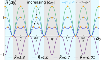
Figure 7: The analytical function $R(\alpha_{0})$, given by Eq. (104), for four distinct values of the parameter $\hat{R}=R_{1}/2R_{2}$. Due to the condition (53), relevant for $\hat{R}\geq 0$, the solution is restricted to either the blue or the gray regions. The evolution of the maximum is indicated by the black arrows as $\hat{R}$ is decreased—or, likewise, $|c_{E3}|$ is increased. The two threshold values are given by $\hat{R}=1$ and $\hat{R}=0$.

$$M_{\hat{\boldsymbol{q}},\alpha_{0}}^{(8)} =\frac{1}{c_{E2}^{4}c_{E1}^{5}}-\frac{c_{E2}}{c_{E1}^{2}}\big{(}\Theta^{(4)}\big{)}^{2}-\frac{4c_{A1}\left(\varphi^{(4)}\!-\!\varphi_{0}^{(4)}\right)^{2}}{\left(c_{A1}\!+\!c_{E1}\right)c_{E1}}$$

$$+R_{1}^{(8)}\cos^{2}(3\alpha_{0})-R_{2}^{(8)}\cos^{4}(3\alpha_{0}),$$ (101)

which enforces the fourth-order corrections

$$\Theta^{(4)} \!=0, \varphi^{(4)} \!=\varphi_{0}^{(4)},$$ (102)

with the definitions of $\varphi_{0}^{(4)}$, $R_{1}^{(8)}$ and $R_{2}^{(8)}$ shown in Appendix D. Crucially, the eighth-order expression (101) has an additional $-R_{2}^{(8)}\cos^{4}(3\alpha_{0})$ dependence on $\alpha_{0}$ that is different from the bare term $\cos^{2}(3\alpha_{0})$. The fact that $R_{2}^{(8)}>0$ is important as it allows for a smooth $\alpha_{0}$ evolution.

To see this, we insert the expressions above into the function $R$, Eq. (54), which then becomes

$$R(\alpha_{0}) =R_{0}+R_{1}\cos^{2}(3\alpha_{0})-R_{2}\cos^{4}(3\alpha_{0})$$ (103)

$$=R_{0}+\frac{R_{1}^{2}}{4R_{2}}-R_{2}\left[\cos^{2}(3\alpha_{0})-\frac{R_{1}}{2R_{2}}\right]^{2},$$ (104)

with:

$$R_{0} =\frac{1}{c_{E1}}\sum_{n=0}^{4}\frac{c_{E3}^{2n}}{c_{E2}^{n}c_{E1}^{n}},$$ (105)

$$R_{1} =\frac{1}{2\tilde{\kappa}_{1}^{2}}-R_{1}^{(4)}c_{E3}^{4}-R_{1}^{(6)}c_{E3}^{6}+R_{1}^{(8)}c_{E3}^{8},$$ (106)

$$R_{2} =R_{2}^{(8)}c_{E3}^{8}.$$ (107)

Note that a factor of $1/\kappa_{1}^{2}$ was absorbed into the function $R(\alpha_{0})$ for convenience. Maximization of Eq. (104) leads to three distinct regimes, depending on the value of the parameter $\hat{R}=\frac{R_{1}}{2R_{2}}$. We find

$$1 <\hat{R}, \rightarrow \cos(3\alpha_{0}) =\pm 1,$$ (108)

$$0\leq\hat{R} \leq 1, \rightarrow \cos(3\alpha_{0}) =\pm\sqrt{\hat{R}},$$ (109)

$$\hat{R} <0, \rightarrow \cos(3\alpha_{0}) =0.$$ (110)

The function $R(\alpha_{0})$, Eq. (104), is depicted in Fig. 7 for four values of $\hat{R}$. Because of the condition (53), valid solutions for the nematic director in the case $\hat{R}\geq 0$ lie either in the gray or in the blue shaded regions, depending on the sign of the cubic parameter $g$. As $\hat{R}$ is decreased—or $|c_{E3}|$ is increased—the number of maxima doubles once $\hat{R}$ falls below the threshold $\hat{R}=1$. We emphasize that the rotation can still happen within the perturbative regime of $|c_{E3}|$, as long as $\tilde{\kappa}_{1}^{-1}\sim|c_{E3}|^{2}\ll 1$. The evolution of the nematic director angle $\alpha_{0}$ with $\hat{R}$ is plotted in Fig. 8, with the three phases identified through the colored background. To make the comparison with the numerical solution more transparent, we added in Fig. 2(a) the curves $c_{E3}\left(\kappa_{1}\right)$ corresponding to the two threshold values, $\hat{R}=0$ and $\hat{R}=1$, which separate the three different regimes for the nematic director. Note that the analytic results quantitatively capture the numerical ones when the threshold value for $c_{E3}$ is small, which corresponds to larger $\tilde{\kappa}_{1}$. Moreover, in agreement with the numerical solution, each nematic director $\alpha_{0}$ is associated with four soft phonon directions given by $N_{0}=\{1,3,5,7\}$. The actual momentum directions $\hat{\boldsymbol{q}}_{0}$ can be computed in a straightforward way via Eqs. (93), (96), (98), (100) and (102).

[][]

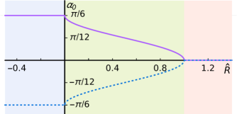
Figure 8: The nematic director $\alpha_{0}$ that maximizes Eq. (104) as a function of $\hat{R}=R_{1}/2R_{2}$. The trends displayed here coincide with those obtained from the numerical solutions depicted in Fig. 3.

[][]

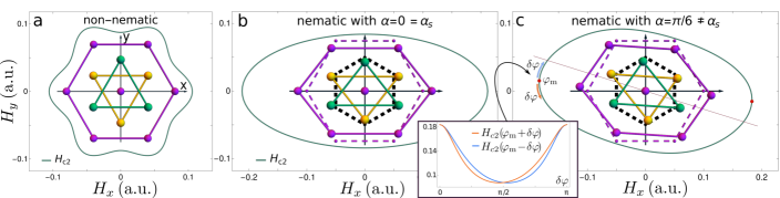
Figure 9: Shape of the in-plane upper critical field $H_{c2}$ superimposed to the schematic distortion of the unit cell. (a) Without nematic order, the upper critical field is sixfold symmetric and respects all of the trigonal point group symmetries. (b) With nematic order and $\alpha=\alpha_{s}$, the shape of $H_{c2}$ is a twofold symmetric ellipse, and the accompanying lattice distortion is monoclinic. (c) With a rotated nematic director ($\alpha\neq\alpha_{s}$), the residual in-plane twofold symmetry of $H_{c2}$ is lost, and the accompanying lattice distortion is triclinic. The main axis of $H_{c2}$ rotates by $\text{-}\alpha/2$ (red line), and the ellipse is deformed, as highlighted in the inset. The inset shows the behavior of the functions $H_{c2}(\varphi_{\mathrm{m}}\pm\delta\varphi)$, which correspond to a clockwise and a counterclockwise sweeping of the $H_{c2}$ curve starting from the angle $\varphi_{\mathrm{m}}$ where $H_{c2}$ is maximum. If a residual twofold symmetry was present, the two curves would overlap.

IV Experimental manifestations in doped $\mathrm{Bi}{}_{2}\mathrm{Se}{}_{3}$

Having established that nemato-elastic interactions in trigonal lattices tend to rotate the nematic director away from high-symmetry directions ($\alpha\neq\alpha_{s}$), we now discuss some of the experimentally observable consequences in the context of the topological superconductor $A\mathrm{{}_{x}Bi_{2}Se_{3}}$. As explained above, using the elastic constant values extracted from first-principles for $\mathrm{Bi_{2}Se_{3}}$ (Gao et al., 2016) (black dotted line in Fig. 2), we expect the nematic director to be rotated in this compound. The degree of rotation depends on the nemato-elastic coupling constants $\tilde{\kappa}_{i}$, whose values are currently not known.

The first consequence of a rotated director is the breaking of the residual $C_{2x}$ (twofold rotation with respect to an in-plane axis) symmetry of the point group $\mathsf{D_{3d}}$. While any non-zero $|\boldsymbol{\Phi}^{E_{g}}|$ breaks $C_{3z}$ (threefold rotation with respect to an out-of-plane axis), the $C_{2x}$ symmetry is only broken when $\alpha\neq\alpha_{s}$. To see this, we study the invariance of a generic nematic order parameter $\boldsymbol{\Phi}^{E_{g}}$ upon the transformation of the group elements $g\in\mathsf{D_{3d}}$,

$$\mathcal{R}_{E_{g}}(g)\,\boldsymbol{\Phi}^{E_{g}} =\boldsymbol{\Phi}^{E_{g}},$$ (111)

with the $E_{g}$-transformation matrices $\mathcal{R}_{E_{g}}(g)$. Depending on whether $\alpha$ aligns with a high-symmetry direction or not, the residual symmetry group $\mathcal{G}$ is different. In particular:

$$\mathcal{G}_{\alpha=\alpha_{s}} =\mathsf{C_{2h}}=\{E,I,C_{2x},IC_{2x}\},$$ (112)

$$\mathcal{G}_{\alpha\neq\alpha_{s}} =\mathsf{C_{I}}\;\;=\{E,I\}.$$ (113)

Here, $E$ denotes the identity and $I$, inversion. Thus, for a rotated director ($\alpha\neq\alpha_{s}$), as expected for doped $\mathrm{Bi_{2}Se_{3}}$, there is no residual twofold symmetry axis. The first consequence of this result is that the nematic transition triggers a triclinic lattice distortion, rather than a monoclinic distortion as in the case of $\alpha=\alpha_{s}$. While the lattice distortion may be very small, it would be interesting to perform high-resolution x-ray measurements to try to resolve between a monoclinic or a triclinic lattice structure. The breaking of the $C_{2x}$ symmetry should also be manifested in any physical quantity that depends on in-plane directions, such as the in-plane $H_{c2}$, the penetration depth, and the thermal conductivity. Perhaps the most accessible of these quantities is the in-plane upper critical field $H_{c2}$.

IV.1 Upper critical field

For a nematic director aligned along the high-symmetry directions, $\alpha=\alpha_{s}$, the azimuthal function $H_{c2}(\varphi_{B})$, where $\varphi_{B}$ is the in-plane angle with respect to the $x$-axis, has an elliptical shape with the major axis oriented along (or perpendicular to) $\text{-}\alpha/2$, see (Venderbos et al., 2016a; Hecker, 2020). However, once $\alpha\neq\alpha_{s}$, $H_{c2}(\varphi_{B})$ no longer has a twofold symmetry axis. To illustrate this behavior, we follow Refs. (Venderbos et al., 2016a; Hecker, 2020) and compute $H_{c2}$, with the detailed derivation shown in Appendix E. The results are shown in the three panels of Fig. 9. In the non-nematic phase [panel (a)], $H_{c2}(\varphi_{B})$ has a sixfold symmetric shape. In the nematic phase with $\alpha=\alpha_{s}$, shown in panel (b), $H_{c2}$ displays an approximately elliptical shape, being invariant upon an in-plane twofold rotation about a high-symmetry axis ($C_{2x}$). The orientation of the ellipse can be obtained from the approximated analytical expression

$$H_{c2} \approx\frac{H_{c2}^{0}}{1+\frac{1}{2}\hat{\mathsf{d}}_{1}\cos(\alpha+2\varphi_{B})},$$ (114)

with the details provided in the Appendix E. In Eq. (114) the contributions associated with the threefold rotational symmetry are neglected. Lastly, when the nematic director unlocks from the high-symmetry directions ($\alpha\neq\alpha_{s}$), as depicted in panel (c) and its inset, the elliptical shape of $H_{c2}$ is distorted and no longer symmetric under any in-plane twofold rotation. The shape of $H_{c2}$ in panel (c) can be understood as a superposition of a rotated ellipse [see Eq. (114)] and the underlying sixfold symmetric pattern illustrated in panel (a). While the lack of $C_{2x}$ symmetry is a robust prediction of the model, the degree in which the ellipse of panel (b) is distorted when $\alpha\neq\alpha_{s}$ can be rather small. For instance, in panel (c), the nematic director was chosen to be aligned with an “anti-symmetry” direction, where the effect is the strongest. The absence of any twofold symmetry in the $H_{c2}$ curve is emphasized in the inset of panel (c), where the two curves $H_{c2}(\varphi_{\mathrm{m}}\pm\delta\varphi)$ are plotted as functions of $\delta\varphi$, with $\varphi_{\mathrm{m}}$ denoting the angle where $H_{c2}$ is maximal. Since the “clockwise” and “counterclockwise” curves do not overlap, $H_{c2}$ lacks twofold symmetry with respect to any in-plane axes. In all three panels, we also show schematically the symmetry of the unit cell in each case, corresponding to trigonal [non-nematic, panel (a)], monoclinic [nematic with $\alpha=\alpha_{s}$, panel (b)], and triclinic [nematic with $\alpha\neq\alpha_{s}$, panel (c)].

[][]

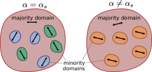
Figure 10: In the case $\alpha=\alpha_{s}$, the system is expected to form one majority nematic domain, e.g. $\alpha=0$ that is accompanied by minority domains randomly composed of the remaing two states, $\alpha\in\{\frac{2\pi}{3},\frac{4\pi}{3}\}$. In the case $\alpha\neq\alpha_{s}$, there are six non-equivalent nematic directors. The system establishes one majority domain, e.g. $\alpha=\delta$ with $0<\delta<\pi/3$. Then, the surface energy $\sigma(\delta,-\delta)$ between adjacent domains, $\alpha=\delta$ and $\alpha=-\delta$, is expected to be smaller than the surface energy between other domains, e.g. $\sigma(\delta,\frac{2\pi}{3}+\delta)$. As a result, the minority domains are expected to be dominated by the $\alpha=-\delta$ domains.

IV.2 Domain formation

The unlocking of the nematic director also has potential implications for domain formation, as illustrated in Fig. 10. Consider the surface energy cost $\sigma(\alpha_{1},\alpha_{2})$ to form two neighboring domains with directors $\alpha_{1}$ and $\alpha_{2}$. In the case $\alpha=\alpha_{s}$, the three possible directors have the same angular separation, and we expect the surface energies between any two domains to be equal. As a result, in the equilibrium state, one director is chosen as the majority domain, with the other two orientations randomly forming minority domains, see Fig. 10 (left panel). In the case $\alpha\neq\alpha_{s}$, however, there are six degenerate directors that can be parametrized as $\alpha\in\{\pm\delta,\frac{2\pi}{3}\pm\delta,\frac{4\pi}{3}\pm\delta\}$, with $0<\delta<\frac{\pi}{3}$. Given an arbitrary director (say $+\delta$) there is an adjacent director that has a lower angular separation than any other director (in this case, $-\delta$). As a result, we expect the surface energy between domains with adjacent directors to be smaller than the surface energy between domains with distant directors, e.g. $\sigma(\delta,-\delta)<\sigma(\delta,\frac{2\pi}{3}+\delta)$. As a result, for a given majority domain, e.g. $\alpha=\delta$, the minority domains in equilibrium should be dominated by the $\alpha=-\delta$ domain, see Fig. 10 (right panel). An interesting question, which is however outside of the scope of this paper, is if these results also affect the typical size of the nematic domains in a macroscopic sample.

IV.3 Gap structure

The rotation of the nematic director angle also has a direct impact on the gap structure, and particularly on the presence or absence of nodal quasi-particles. As explained in the Introduction, the nematic superconducting gap transforms according to the two-dimensional irreducible representation $E_{u}$ and can be parametrized according to:

$$\boldsymbol{\Delta} =\left(\begin{array}[]{c}\Delta_{1}\\ \Delta_{2}\end{array}\right)=|\boldsymbol{\Delta}|e^{\mathsf{i}\vartheta}\left(\begin{array}[]{c}\cos\frac{\alpha}{2}\\ -\sin\frac{\alpha}{2}\end{array}\right),$$ (119)

where $\vartheta\in[0,2\pi)$ is the global phase and $\alpha\in[0,2\pi)$, the nematic director angle. Without the effects of the phonon renormalization, the director angle $\alpha$ aligns with one of the high-symmetry directions given by either $\alpha_{s}^{(1)}\in\{0,2,4\}\frac{\pi}{3}$ or $\alpha_{s}^{(2)}\in\{1,3,5\}\frac{\pi}{3}$. As discussed in Ref. (Fu, 2014), $\boldsymbol{\Delta}(\alpha_{s}^{(1)})$ describes a fully-gapped superconducting state whereas $\boldsymbol{\Delta}(\alpha_{s}^{(2)})$ is a nodal pairing state with point nodes protected by the $C_{2x}$ symmetry of the system. Following the arguments of Ref. (Fu, 2014), the stability of the nodes can be seen by noting that the $\boldsymbol{d}$-vector that describes this triplet superconducting state is given in terms of $\Delta_{1}$ and $\Delta_{2}$ according to:

$$\boldsymbol{d}(\boldsymbol{k}) =\Delta_{1}\boldsymbol{d}_{1}(\boldsymbol{k})+\Delta_{2}\boldsymbol{d}_{2}(\boldsymbol{k}),$$ (120)

with the individual $\boldsymbol{d}_{j}$-vectors satisfying $\boldsymbol{d}_{j}(-\boldsymbol{k})=-\boldsymbol{d}_{j}(\boldsymbol{k})$ where $j=\{1,2\}$. Nodes emerge when all three components of $\boldsymbol{d}(\boldsymbol{k})$ vanish on either points or lines along the Fermi surface, which usually only happens due to an underlying crystallographic symmetry (Blount, 1985; Fu, 2014). Indeed, under the $C_{2x}$ symmetry operation, the $\boldsymbol{d}_{j}$-vectors transform as

$$\boldsymbol{d}_{1}[\mathcal{R}_{v}^{\dagger}(C_{2x})\boldsymbol{k}] =\mathcal{R}_{v}^{\dagger}(C_{2x})\boldsymbol{d}_{1}(\boldsymbol{k}),$$ (121)

$$\boldsymbol{d}_{2}[\mathcal{R}_{v}^{\dagger}(C_{2x})\boldsymbol{k}] =-\mathcal{R}_{v}^{\dagger}(C_{2x})\boldsymbol{d}_{2}(\boldsymbol{k}),$$ (122)

with $\mathcal{R}_{v}^{\dagger}(C_{2x})$ denoting the transformation matrix of the vector representation. Using the result $\mathcal{R}_{v}^{\dagger}(C_{2x})\boldsymbol{k}_{yz}=-\boldsymbol{k}_{yz}$, which holds for any momentum $\boldsymbol{k}_{yz}=(0,k_{y},k_{z})^{T}$ in the $\left(k_{y},k_{z}\right)$ plane, i.e. the $IC_{2x}$ mirror plane, Eqs. (121)-(122) become

$$0 =[\mathbbm{1}\!+\!\mathcal{R}_{v}^{\dagger}(C_{2x})]\,\boldsymbol{d}_{1}(\boldsymbol{k}_{yz}), 0 =[\mathbbm{1}\!-\!\mathcal{R}_{v}^{\dagger}(C_{2x})]\,\boldsymbol{d}_{2}(\boldsymbol{k}_{yz}).$$

This results in $d_{1x}(\boldsymbol{k}_{yz})=0$ and $d_{2y}(\boldsymbol{k}_{yz})=d_{2z}(\boldsymbol{k}_{yz})=0$, i.e. the vector $\boldsymbol{d}_{1}(\boldsymbol{k}_{yz})$ is parallel to the $\left(k_{y},k_{z}\right)$ plane, whereas $\boldsymbol{d}_{2}(\boldsymbol{k}_{yz})$ is normal to it. This has important consequences for $\boldsymbol{d}_{2}(\boldsymbol{k}_{yz})$, since the odd-parity constraint, $d_{2x}(-\boldsymbol{k}_{yz})=-d_{2x}(\boldsymbol{k}_{yz})$, implies that $d_{2x}(\boldsymbol{k}_{yz})$ vanishes at least along one line in the $\left(k_{y},k_{z}\right)$ plane. The intersection of this line with the Fermi surface then leads to a point node – assuming, of course, that the Fermi surface also crosses this plane. Thus, the twofold symmetry $C_{2x}$, via (122), forces the superconducting state described by the order parameter $\boldsymbol{\Delta}(\alpha_{s}^{(2)}=\pi)=-|\boldsymbol{\Delta}|e^{\mathsf{i}\vartheta}(0,1)^{T}$, as well as its $\alpha_{s}^{(2)}$ partners, to have point nodes.

Therefore, when the nematic director angle unlocks from the high-symmetry directions, $\alpha\neq\alpha_{s}^{(1,2)}$, the superconducting order parameter (119) rotates accordingly and the system loses the symmetry element $C_{2x}$ that protects the point nodes, see Eq. (113). As a result, the superconducting state becomes fully gapped (Fu, 2014). To show this explicitly, we consider the well-established $\boldsymbol{k}\cdot\boldsymbol{p}$ Hamiltonian for Bi₂Se₃ (Zhang et al., 2009; Liu et al., 2010; Venderbos et al., 2016b) and write down an expression for the magnitude of the $\boldsymbol{d}$-vector following the approach in Ref. (Venderbos et al., 2016b) (see Appendix F for details). We obtain

$$\frac{|\boldsymbol{d}(\boldsymbol{k})|^{2}}{|\boldsymbol{\Delta}|^{2}} =\big{(}\hat{f}_{\boldsymbol{k}}^{z}\big{)}^{2}+\hat{M}_{\boldsymbol{k}}^{2}\big{(}\hat{f}_{\boldsymbol{k}}^{C_{3}}\big{)}^{2}+\Big{(}\hat{f}_{\boldsymbol{k}}^{x}\sin\frac{\alpha}{2}+\hat{f}_{\boldsymbol{k}}^{y}\cos\frac{\alpha}{2}\Big{)}^{2}$$

$$\!\!\!\!\!\!\!\!\!\!\!\!\!\!+\big{(}\hat{f}_{\boldsymbol{k}}^{C_{3}}\big{)}^{2}\frac{\hat{\boldsymbol{f}}_{\boldsymbol{k}}^{2}\!+\!2|\hat{M}_{\boldsymbol{k}}|(1\!+\!|\hat{M}_{\boldsymbol{k}}|)}{(1\!+\!|\hat{M}_{\boldsymbol{k}}|)^{2}}\Big{(}\hat{f}_{\boldsymbol{k}}^{x}\cos\!\frac{\alpha}{2}-\hat{f}_{\boldsymbol{k}}^{y}\sin\!\frac{\alpha}{2}\Big{)}^{2},$$ (123)

which is a sum of individually positive contributions. Hence, the gap only vanishes when the three terms

$$0 =\hat{f}_{\boldsymbol{k}}^{z}, 0 =\hat{f}_{\boldsymbol{k}}^{C_{3}}, 0 =\hat{f}_{\boldsymbol{k}}^{x}\sin\frac{\alpha}{2}+\hat{f}_{\boldsymbol{k}}^{y}\cos\frac{\alpha}{2},$$ (124)

are simultaneously equal to zero. Note that $\hat{M}_{\boldsymbol{k}}$ is generally different from zero. While the full expressions for these functions are given in Appendix F, the important point is that $\hat{f}_{\boldsymbol{k}}^{z}$ transforms as the $A_{2u}$ irreducible representation; $(\hat{f}_{\boldsymbol{k}}^{x},\,\hat{f}_{\boldsymbol{k}}^{y})$, as $E_{u}$; and $\hat{f}_{\boldsymbol{k}}^{C_{3}}$, as $A_{1u}$. Consequently, $\hat{f}_{\boldsymbol{k}}^{C_{3}}$ only vanishes along the three momentum-space directions $k_{x}=0$ and $k_{x}=\pm\sqrt{3}k_{y}$, which define the three mirror planes. Focusing on the $k_{x}=0$ plane, the requirement $\hat{f}_{\boldsymbol{k}}^{z}=0$ implies $k_{z}\sim k_{y}^{3}$, which defines a line within the $k_{x}=0$ plane. Along this line, because $\hat{f}_{\boldsymbol{k}}^{x}=0$ and $\hat{f}_{\boldsymbol{k}}^{y}\neq 0$, the last condition in (124) is satisfied only for $\alpha=\pi$. Repeating the same steps for the other two planes, we find that the last condition is satisfied for specific values of the nematic director

$$k_{x} =0 \rightarrow\alpha =\pi,$$

$$k_{x} =\sqrt{3}k_{y} \rightarrow\alpha =5\pi/3,$$

$$k_{x} =-\sqrt{3}k_{y} \rightarrow\alpha =\pi/3,$$

which coincide with the three high-symmetry directions $\alpha=\alpha_{s}^{(2)}$. Any other director angle $\alpha\neq\alpha_{s}^{(2)}$ thus necessarily leads to a full superconducting gap, as first shown in Ref. (Fu, 2014). For the parameters of $\mathrm{Bi_{2}Se_{3}}$, because the director is unlocked from the high-symmetry directions due to the phonon renormalization, we expect always a fully gapped superconducting state.

V Concluding remarks

In lattices with threefold or sixfold rotational symmetry, the nematic order parameter is defined not only by an amplitude, but also by the orientation of the nematic director $\alpha$. Usually, one expects this director to align with a high-symmetry direction of the crystal, $\alpha=\alpha_{s}$. In this work, we have shown that the orientation of the nematic director can be fundamentally changed by the nemato-elastic coupling, due to the long-range nematic interactions mediated by the acoustic phonons. This is the case for any $Z_{3}$-Potts nematic order in trigonal lattices with point groups $\mathsf{D_{3d}}$, $\mathsf{D_{3}}$, $\mathsf{C_{3v}}$, $\mathsf{S_{6}}$ and $\mathsf{C_{3}}$, but not for hexagonal lattices with point groups $\mathsf{D_{6h}}$, $\mathsf{D_{6}}$, $\mathsf{C_{6h}}$, $\mathsf{C_{6v}}$, $\mathsf{D_{3h}}$, $\mathsf{C_{3h}}$ and $\mathsf{C_{6}}$. This is a consequence of the fact that only in the former groups the in-plane shear strain $\boldsymbol{\epsilon}^{E_{g},1}=(\epsilon_{11}-\epsilon_{22},-2\epsilon_{12})^{T}$ and out-of-plane shear strain $\boldsymbol{\epsilon}^{E_{g},2}=(2\epsilon_{23},-2\epsilon_{31})^{T}$ transform as the same two-dimensional irreducible representation, which results in the emergence of a symmetry-allowed elastic constant $c_{14}$. By minimizing the acoustic-phonon renormalized nematic action, we found that when either $c_{14}$ or the nemato-elastic coupling overcomes a threshold value, the nematic director unlocks from the high-symmetry directions ($\alpha\neq\alpha_{s}$), resulting in the breaking of a residual twofold rotational symmetry with respect to an in-plane axis, $C_{2x}$.

In doped $\mathrm{Bi_{2}Se_{3}}$, with point group $\mathsf{D_{3d}}$, the value of $c_{14}$ extracted from first-principles calculations place the system in the regime where the nematic director is rotated with respect to the high-symmetry directions. In this regime, the number of non-equivalent nematic directors doubles from three to six, and each director is associated with four momentum-space directions for which the nematic susceptibility is large. Moreover, we showed that the breaking of $C_{2x}$ is manifested not only by a triclinic distortion of the lattice, but also by an in-plane critical field curve that retains only inversion symmetry and by the complete removal of any point nodes that could otherwise exist inside the superconducting state. Experimental verification of these features would provide strong evidence for the fundamental impact of the lattice on the nematic superconducting state of doped $\mathrm{Bi_{2}Se_{3}}$. In this regard, we note that Refs. (Du et al., 2017; Kuntsevich et al., 2018, 2019; Tao et al., 2018) reported a mismatch between the long-axis of the in-plane $H_{c2}$ “ellipse” and the lattice axes, which would be consistent with our model.

Appendix A Irreducible representations of the shear strain doublets

In this appendix, we discuss the conditions under which the two strain doublets $\boldsymbol{\epsilon}^{(1)}=(\epsilon_{11}-\epsilon_{22},-2\epsilon_{12})^{T}$ (in-plane shear) and $\boldsymbol{\epsilon}^{(2)}=(2\epsilon_{23},-2\epsilon_{31})^{T}$ (out-of-plane shear) transform as the same irreducible representations of a point group for which $C_{3z}$ is a symmetry element. To this end, we consider the largest hexagonal point group $\mathsf{D_{6h}}$, which has $24$ symmetry elements that can be conveniently written as

$$\mathsf{D_{6h}} =\{E,C_{3z}^{\pm 1}\}\otimes\{E,C_{2x}\}\otimes\{E,C_{2z}\}\otimes\{E,I\}.$$ (125)

Among the elements in the brackets, the only element under which the strain doublets $\boldsymbol{\epsilon}^{(1)}$ and $\boldsymbol{\epsilon}^{(2)}$ transform differently is $C_{2z}$. Hence, the presence of any element that can be expressed in terms of $C_{2z}$ (e.g. $C_{2z}$, $IC_{2z}$, $C_{2x}C_{2z}$, etc.) prohibits the two doublets from belonging to the same irreducible representation. Given the representation (125), it is straightforward to construct the corresponding subgroups. Note that the block $\{E,C_{3z}^{\pm 1}\}$ is responsible for the degeneracy that enforces the existence of the doublets in the first place. Thus, we will only consider subgroups that contain this main block $\{E,C_{3z}^{\pm 1}\}$. There are five subgroups that contain $12$ symmetry elements:

$$\mathsf{D_{6}} =\{E,C_{3z}^{\pm 1}\}\otimes\{E,C_{2x}\}\otimes\{E,C_{2z}\},$$

$$\boldsymbol{\mathsf{D_{3d}}} =\{E,C_{3z}^{\pm 1}\}\otimes\{E,C_{2x}\}\otimes\{E,I\},$$

$$\mathsf{C_{6h}} =\{E,C_{3z}^{\pm 1}\}\otimes\{E,C_{2z}\}\otimes\{E,I\},$$

$$\mathsf{D_{3h}} =\{E,C_{3z}^{\pm 1}\}\otimes\{E,C_{2x}\}\otimes\{E,IC_{2z}\},$$

$$\mathsf{C_{6v}} =\{E,C_{3z}^{\pm 1}\}\otimes\{E,IC_{2x}\}\otimes\{E,C_{2z}\}.$$

The only group where $\boldsymbol{\epsilon}^{(1)}$ and $\boldsymbol{\epsilon}^{(2)}$ transform under the same IR (represented in boldface), i.e. where the element $C_{2z}$ is absent, is the point group $\mathsf{D_{3d}}$. The subgroups that contain $6$ elements are:

$$\boldsymbol{\mathsf{D_{3}}} =\{E,C_{3z}^{\pm 1}\}\otimes\{E,C_{2x}\},$$

$$\boldsymbol{\mathsf{S_{6}}} =\{E,C_{3z}^{\pm 1}\}\otimes\{E,I\},$$

$$\mathsf{C_{6}} =\{E,C_{3z}^{\pm 1}\}\otimes\{E,C_{2z}\},$$

$$\mathsf{C_{3h}} =\{E,C_{3z}^{\pm 1}\}\otimes\{E,IC_{2z}\},$$

$$\boldsymbol{\mathsf{C_{3v}}} =\{E,C_{3z}^{\pm 1}\}\otimes\{E,IC_{2x}\}.$$

Lastly, there is only one subgroup with $3$ elements:

$$\boldsymbol{\mathsf{C_{3}}} =\{E,C_{3z}^{\pm 1}\}.$$

Note that the set of the five boldface point groups form the full set of trigonal point groups.

Appendix B Dynamic matrix for a trigonal lattice

The dynamic matrix $D_{ij}(\boldsymbol{q})=\sum_{i^{\prime},j^{\prime}}\mathcal{C}_{ii^{\prime}jj^{\prime}}q_{i^{\prime}}q_{j^{\prime}}$ introduced in Eq. (24), with $\{i,j,i^{\prime},j^{\prime}\}\in\{1,2,3\}$, satisfies $D(-\boldsymbol{q})=D(\boldsymbol{q})$ and $D^{T}(\boldsymbol{q})=D(\boldsymbol{q})$. In the $\mathsf{D_{3d}}$ point group, the matrix elements are given by

$$D_{11}(\boldsymbol{q}) =F_{a,\boldsymbol{q}}^{A_{1g}}\!+\!F_{a,\boldsymbol{q}}^{E_{g},1}\!+\!\frac{1}{\sqrt{3}}F_{b,\boldsymbol{q}}^{A_{1g}}, D_{12}(\boldsymbol{q}) =-F_{a,\boldsymbol{q}}^{E_{g},2},$$

$$D_{22}(\boldsymbol{q}) =F_{a,\boldsymbol{q}}^{A_{1g}}\!-\!F_{a,\boldsymbol{q}}^{E_{g},1}\!+\!\frac{1}{\sqrt{3}}F_{b,\boldsymbol{q}}^{A_{1g}}, D_{13}(\boldsymbol{q}) =-F_{b,\boldsymbol{q}}^{E_{g},2},$$

$$D_{33}(\boldsymbol{q}) =F_{a,\boldsymbol{q}}^{A_{1g}}\!-\!\frac{2}{\sqrt{3}}F_{b,\boldsymbol{q}}^{A_{1g}}, D_{23}(\boldsymbol{q}) =F_{b,\boldsymbol{q}}^{E_{g},1}.$$

Here, we defined

$$F_{a,\boldsymbol{q}}^{A_{1g}} =\frac{c_{A1}+2c_{E1}+c_{E2}}{3}f_{\boldsymbol{q}}^{A1}+\frac{c_{A2}+2c_{E2}}{3}f_{\boldsymbol{q}}^{A2},$$

$$F_{b,\boldsymbol{q}}^{A_{1g}} =\frac{c_{A1}+2c_{E1}-2c_{E2}}{2\sqrt{3}}f_{\boldsymbol{q}}^{A1}+\frac{c_{E2}-c_{A2}}{\sqrt{3}}f_{\boldsymbol{q}}^{A2},$$

$$\boldsymbol{F}_{a,\boldsymbol{q}}^{E_{g}} =\frac{c_{A1}}{2}\boldsymbol{f}_{\boldsymbol{q}}^{E1}+c_{E3}\boldsymbol{f}_{\boldsymbol{q}}^{E2},$$

$$\boldsymbol{F}_{b,\boldsymbol{q}}^{E_{g}} =c_{E3}\boldsymbol{f}_{\boldsymbol{q}}^{E1}+\frac{c_{A3}+c_{E2}}{2}\boldsymbol{f}_{\boldsymbol{q}}^{E2},$$

as well as

$$f_{\boldsymbol{q}}^{A1} =q_{x}^{2}+q_{y}^{2}, f_{\boldsymbol{q}}^{A2} =q_{z}^{2},$$

$$\boldsymbol{f}_{\boldsymbol{q}}^{E1} =\left(\begin{array}[]{c}q_{x}^{2}-q_{y}^{2}\\ -2q_{x}q_{y}\end{array}\right), \boldsymbol{f}_{\boldsymbol{q}}^{E2} =\left(\begin{array}[]{c}2q_{y}q_{z}\\ -2q_{x}q_{z}\end{array}\right).$$

We obtain the eigenvalues:

$$\omega_{j,\boldsymbol{q}}^{2} =F_{a,\boldsymbol{q}}^{A_{1}}-\frac{1}{3}x_{j,\boldsymbol{q}},$$

with

$$\left(\begin{array}[]{c}x_{1,\boldsymbol{q}}\\ x_{2,\boldsymbol{q}}\\ x_{3,\boldsymbol{q}}\end{array}\right) =-2\sqrt{3}F_{\boldsymbol{q}}\left(\begin{array}[]{c}\cos\left(\frac{\eta_{\boldsymbol{q}}}{3}\right)\\ \cos\left(\frac{\eta_{\boldsymbol{q}}}{3}+\frac{2\pi}{3}\right)\\ \cos\left(\frac{\eta_{\boldsymbol{q}}}{3}-\frac{2\pi}{3}\right)\end{array}\right),$$

and

$$F_{\boldsymbol{q}} =\sqrt{(F_{b,\boldsymbol{q}}^{A_{1g}})^{2}+(\boldsymbol{F}_{a,\boldsymbol{q}}^{E_{g}})^{2}+(\boldsymbol{F}_{b,\boldsymbol{q}}^{E_{g}})^{2}},$$

$$\mathsf{d}_{\boldsymbol{q}} =\det D(\boldsymbol{q})\Big{|}_{F_{a,\boldsymbol{q}}^{A_{1g}}=0}$$

$$=\frac{1}{\sqrt{3}}F_{b,\boldsymbol{q}}^{A_{1g}}\Big{(}2(\boldsymbol{F}_{a,\boldsymbol{q}}^{E_{g}})^{2}\!-\!(\boldsymbol{F}_{b,\boldsymbol{q}}^{E_{g}})^{2}\!-\!\frac{2}{3}(F_{b,\boldsymbol{q}}^{A_{1g}})^{2}\Big{)}$$

$$\quad-\boldsymbol{F}_{a,\boldsymbol{q}}^{E_{g}}\cdot\left(\begin{array}[]{c}(F_{b,\boldsymbol{q}}^{E_{g},1})^{2}-(F_{b,\boldsymbol{q}}^{E_{g},2})^{2}\\ -2F_{b,\boldsymbol{q}}^{E_{g},1}F_{b,\boldsymbol{q}}^{E_{g},2}\end{array}\right),$$

$$\eta_{\boldsymbol{q}} =\arccos\left(\frac{3\sqrt{3}}{2}\frac{\mathsf{d}_{\boldsymbol{q}}}{F_{\boldsymbol{q}}^{3}}\right).$$

The corresponding eigenvectors can be generically written as

$$\hat{\boldsymbol{e}}_{\boldsymbol{q}}^{(j)} =\frac{\mathrm{sign}(q_{j})}{|\boldsymbol{u}_{j,\boldsymbol{q}}|}\left(\begin{array}[]{c}u_{j,\boldsymbol{q}}^{(1)}\\ u_{j,\boldsymbol{q}}^{(2)}\\ u_{j,\boldsymbol{q}}^{(3)}\end{array}\right),$$ (129)

where we defined

$$u_{j,\boldsymbol{q}}^{(1)} =3(F_{b,\boldsymbol{q}}^{E_{g},1})^{2}-2\sqrt{3}F_{b,\boldsymbol{q}}^{A_{1g}}F_{a,\boldsymbol{q}}^{E_{g},1}+2(F_{b,\boldsymbol{q}}^{A_{1}})^{2}$$

$$\quad+\Big{(}\frac{1}{\sqrt{3}}F_{b,\boldsymbol{q}}^{A_{1g}}+F_{a,\boldsymbol{q}}^{E_{g},1}\Big{)}x_{j,\boldsymbol{q}}-\frac{1}{3}x_{j,\boldsymbol{q}}^{2},$$

$$u_{j,\boldsymbol{q}}^{(2)} =3F_{b,\boldsymbol{q}}^{E_{g},1}F_{b,\boldsymbol{q}}^{E_{g},2}\!+\!F_{a,\boldsymbol{q}}^{E_{g},2}\big{(}2\sqrt{3}F_{b,\boldsymbol{q}}^{A_{1g}}-x_{j,\boldsymbol{q}}\big{)},$$

$$u_{j,\boldsymbol{q}}^{(3)} =3\big{(}F_{a,\boldsymbol{q}}^{E_{g},2}F_{b,\boldsymbol{q}}^{E_{g},1}\!+\!F_{b,\boldsymbol{q}}^{E_{g},2}F_{a,\boldsymbol{q}}^{E_{g},1}\big{)}\!$$

$$\quad-\!F_{b,\boldsymbol{q}}^{E_{g},2}\big{(}\!\sqrt{3}F_{b,\boldsymbol{q}}^{A_{1g}}\!+\!x_{j,\boldsymbol{q}}\big{)}.$$

The additional function $\mathrm{sign}(q_{j})$ in (129) is necessary to guarantee $\hat{\boldsymbol{e}}_{\boldsymbol{q}}^{(j)}=-\hat{\boldsymbol{e}}_{-\boldsymbol{q}}^{(j)}$.

Appendix C Symmetry-imposed degeneracies of the nematic director

We determine here the set of symmetry-enforced degenerate maxima to the function $R(\hat{\boldsymbol{q}},\alpha_{0})$ in Eq. (51). As discussed in Appendix A, the $\mathsf{D_{3d}}$ point group consists of the $12$ symmetry elements:

$$\mathsf{D_{3d}} =\{E,C_{3z}^{\pm 1}\}\otimes\{E,C_{2x}\}\otimes\{E,I\}.$$

For convenience, we list the transformation matrices of the two-dimensional IRs $E_{g/u}$. For the following elements, the two IRs transform identically,

$$\mathcal{R}_{E_{g/u}}(C_{3z}^{\pm 1}) =\frac{1}{2}\left(\begin{array}[]{cc}-1&\mp\sqrt{3}\\ \pm\sqrt{3}&-1\end{array}\right),$$

$$\mathcal{R}_{E_{g/u}}(C_{2x}) =\left(\begin{array}[]{cc}1&0\\ 0&-1\end{array}\right),$$

$$\mathcal{R}_{E_{g/u}}(C_{2\{A,B\}}) =\frac{1}{2}\left(\begin{array}[]{cc}-1&\mp\sqrt{3}\\ \mp\sqrt{3}&1\end{array}\right),$$

where $C_{2A}=C_{3z}^{-1}C_{2x}$ and $C_{2B}=C_{3z}C_{2x}$. With $\mathcal{R}_{E_{g/u}}(I)=\pm\mathbbm{1}_{2}$, the remaining matrices can be directly read from these expressions. The real-space and momentum-space coordinates transform according to the vector representation $v$ with $\mathcal{R}_{v}(g)=\mathcal{R}_{E_{u}}(g)\oplus\mathcal{R}_{A_{2u}}(g)$ and $g\in\mathsf{D_{3d}}$. Let us rewrite the function $R(\hat{\boldsymbol{q}},\alpha_{0})$ that needs to be maximized,

$$R(\hat{\boldsymbol{q}},\alpha_{0}) =M(\hat{\boldsymbol{q}},\alpha_{0})+\frac{g^{2}\cos^{2}(3\alpha_{0})}{2u},$$ (130)

and the mass function

$$M(\hat{\boldsymbol{q}},\alpha_{0}) =\Pi_{(\boldsymbol{q},0)}^{A_{1g}}+\boldsymbol{\Pi}_{(\boldsymbol{q},0)}^{E_{g}}\cdot\boldsymbol{\mathsf{b}}_{\alpha_{0}}^{E_{g}}\!,$$ (131)

where we introduced the abbreviated notation

$$\boldsymbol{\mathsf{b}}_{\alpha_{0}}^{E_{g}} =\left(\begin{array}[]{c}\cos(2\alpha_{0})\\ -\sin(2\alpha_{0})\end{array}\right),$$ (134)

that transforms according to $E_{g}$. We have

$$\Pi_{(\mathcal{R}_{v}(g)\boldsymbol{q},0)}^{A_{1g}} =\Pi_{(\boldsymbol{q},0)}^{A_{1g}},$$ (135)

$$\boldsymbol{\Pi}_{(\mathcal{R}_{v}(g)\boldsymbol{q},0)}^{E_{g}} =\mathcal{R}_{E_{g}}(g)\,\boldsymbol{\Pi}_{(\boldsymbol{q},0)}^{E_{g}},$$ (136)

for any $g\in\mathsf{D_{3d}}$. Now, we establish the three constraints that relate the degenerate maxima $R(\hat{\boldsymbol{q}}_{0},\alpha_{0})$ with each other. Let us assume $\{\alpha_{0},\hat{\boldsymbol{q}}_{0}\}$ to describe a given maximum.

• Inversion. Since the functions $\Pi_{(\boldsymbol{q},0)}^{A_{1g}}$ and $\boldsymbol{\Pi}_{(\boldsymbol{q},0)}^{E_{g}}$ are invariant upon the inversion operation, the whole function (130) is, such that $R(-\hat{\boldsymbol{q}}_{0},\alpha_{0})$ is a degenerate maximum.

• Three-fold rotation. A variable shift $\alpha_{0}\rightarrow\alpha_{0}\mp\frac{2\pi}{3}$ leaves the second term in (130) invariant, and it shifts

  $$\boldsymbol{\mathsf{b}}_{\alpha_{0}\mp\frac{2\pi}{3}}^{E_{g}} =\mathcal{R}_{E_{g}}(C_{3z}^{\pm 1})\,\boldsymbol{\mathsf{b}}_{\alpha_{0}}^{E_{g}}.$$ (137)

  As for Eqs. (131) and (135)-(136), the shift (137) can be compensated by a momentum rotation with $g=C_{3z}^{\pm 1}$. Then, the function $R$ stays invariant, and it holds

  $$R(\mathcal{R}_{v}(C_{3z})\hat{\boldsymbol{q}}_{0},\alpha_{0}-\frac{2\pi}{3}) =R(\hat{\boldsymbol{q}}_{0},\alpha_{0}),$$ (138)

  $$R(\mathcal{R}_{v}^{-1}(C_{3z})\hat{\boldsymbol{q}}_{0},\alpha_{0}+\frac{2\pi}{3}) =R(\hat{\boldsymbol{q}}_{0},\alpha_{0}).$$ (139)

• Reflection. Let us define the nematic director angle $\alpha_{0}=\alpha_{s}+\delta$ with respect to a high-symmetry direction [recall $\alpha_{s}\in\frac{\pi}{3}\{0,1,2,3,4,5\}$]. Then, the second term in (130) is invariant upon a sign change of the deviation $\delta\rightarrow-\delta$ as $\cos(3\alpha_{0})=\cos(3\alpha_{s})\cos(3\delta)$. For the quantity (134), we obtain

  $$\boldsymbol{\mathsf{b}}_{\alpha_{s}-\delta}^{E_{g}} =\begin{cases}\mathcal{R}_{E_{g}}(IC_{2x})\boldsymbol{\mathsf{b}}_{\alpha_{s}+\delta}^{E_{g}}&,\alpha_{s}\in\{0,3\}\frac{\pi}{3}\\ \mathcal{R}_{E_{g}}(IC_{2B})\boldsymbol{\mathsf{b}}_{\alpha_{s}+\delta}^{E_{g}}&,\alpha_{s}\in\{1,4\}\frac{\pi}{3}\\ \mathcal{R}_{E_{g}}(IC_{2A})\boldsymbol{\mathsf{b}}_{\alpha_{s}+\delta}^{E_{g}}&,\alpha_{s}\in\{2,5\}\frac{\pi}{3}\end{cases}.$$ (140)

  Just like before, the appropriate momentum rotation with $g=IC_{2n_{s}}$ and $n_{s}\in\{x,B,A\}$ chosen according to (140) compensates the transformation (140). As a result, we obtain the degenerate maxima $R(\mathcal{R}_{v}(IC_{2n_{s}})\hat{\boldsymbol{q}}_{0},\alpha_{s}-\delta)=R(\hat{\boldsymbol{q}}_{0},\alpha_{s}+\delta)$. Clearly, this relation is also true for $\delta=0$.

Combined together, the above symmetry constraints lead to twelve degenerate maxima of the function $R$. Importantly, a nematic director $\alpha_{0}=\alpha_{s}+\delta$ with a finite deviation $\delta$ necessarily induces a degenerate maximum with $\alpha_{0}=\alpha_{s}-\delta$. Hence, a finite $\delta\neq 0$ doubles the number of degenerate nematic directors.

Appendix D Details of the analytical approach

In Sec. III.2.1, we introduced the quantities $M_{1}$, $M_{\theta}^{s}$, and $M_{\theta}^{c}$ in Eqs. (72) and (81). The first expression $M_{1}=\kappa_{1}^{2}/(c_{A1}\!+\!c_{E1})$ is obtained by inserting the eigenvalues and eigenvectors associated with the $\hat{\boldsymbol{q}}_{1}$ direction, Eqs. (69)-(71), into the renormalized mass expression (59). To show that $M_{\mathrm{stat}}>M_{1}$, consider $M_{\mathrm{stat}}(c_{E3})$ as a function of $c_{E3}$:

$$M_{\mathrm{stat}}(c_{E3})=\frac{c_{E2}\kappa_{1}^{2}+c_{E1}\kappa_{2}^{2}-2c_{E3}\kappa_{1}\kappa_{2}}{c_{E1}c_{E2}-c_{E3}^{2}}.$$ (141)

First, one finds $M_{1}<M_{\mathrm{stat}}(0)=\frac{\kappa_{1}^{2}}{c_{E1}}+\frac{\kappa_{2}^{2}}{c_{E2}}$ and $M_{1}<M_{\mathrm{stat}}(\pm|c_{E3}|_{\mathrm{max}})\rightarrow+\infty$. Additionally, at the two zeros of the derivative $M_{\mathrm{stat}}^{\prime}(c_{E3})=\left(\kappa_{2}c_{E1}-\kappa_{1}c_{E3}\right)\left(\kappa_{2}c_{E3}-\kappa_{1}c_{E2}\right)/\mathsf{d}_{E}^{2}$, defined through $c_{E3}^{(1)}=\kappa_{2}c_{E1}/\kappa_{1}$ and $c_{E3}^{(2)}=\kappa_{1}c_{E2}/\kappa_{2}$, one similarly obtains $M_{\mathrm{stat}}(c_{E3}^{(1)})>M_{1}$ and $M_{\mathrm{stat}}(c_{E3}^{(2)})>M_{1}$, proving that it always holds $M_{\mathrm{stat}}>M_{1}$.

The quantities $M_{\theta}^{s}$ and $M_{\theta}^{c}$ can be derived in an analogous way using the eigenvalues and eigenvectors associated with the $\hat{\boldsymbol{q}}_{\bar{2}}$ direction:

$$M_{\theta}^{c} =\frac{\kappa_{1}\kappa_{2}\lambda_{2,\theta}}{\tilde{\omega}_{1,\hat{\boldsymbol{q}}_{\bar{2}}}^{2}\tilde{\omega}_{3,\hat{\boldsymbol{q}}_{\bar{2}}}^{2}}\Big{[}(\text{-}1)^{\frac{n_{2}+1}{2}}\!+\!\frac{\kappa_{2}}{\kappa_{1}}(\frac{\lambda_{1,\theta}}{\lambda_{2,\theta}}\!-\!\cot\!\theta)$$

$$\!\!\!\!\!\!\!\!+\!\Big{(}\!\frac{\kappa_{1}}{\kappa_{2}}\!+\!\frac{\kappa_{2}}{\kappa_{1}}\!+\!\frac{\kappa_{2}}{\kappa_{1}}\cot^{2}\!\theta\!-\!2(\text{-}1)^{\!\frac{n_{2}+1}{2}}\!\cot\!\theta\!\Big{)}\!\frac{c_{E2}\!+\!c_{A2}\!\cot^{2}\!\theta}{\lambda_{2,\theta}}\Big{]}\!,$$

$$M_{\theta}^{s} =\frac{\kappa_{1}^{2}+2\kappa_{1}\kappa_{2}(\text{-}1)^{\frac{n_{2}+1}{2}}\cot\!\theta+\kappa_{2}^{2}\cot^{2}\!\theta}{c_{E1}\!+\!2c_{E3}(\text{-}1)^{\frac{n_{2}+1}{2}}\cot\!\theta\!+\!c_{E2}\cot^{2}\!\theta}.$$

We note that $M_{\theta}^{s}$ originates from the second eigenvalue $\tilde{\omega}_{2,\hat{\boldsymbol{q}}_{\bar{2}}}^{2}$, which is also the one that vanishes at the pure structural phase transition. Thus, it is $M_{\theta}^{s}$ that can attain the maximum value $M_{\mathrm{stat}}$. Indeed, the solution of the equation $M_{\theta_{2}}^{s}=M_{\mathrm{stat}}$ is the polar angle $\theta_{2}$ given by Eq. (67).

In Sec. III.2.3, we introduced the functions $A_{\theta}^{\pm}$, $B_{\theta}^{\pm}$ and $C_{\theta}^{\pm}$ that occur in the renormalized mass expression Eq. (86), and which are defined here. Let us recall that the eigenvalues and eigenfrequencies of the dynamical matrix in the $c_{E3}=0$ case are given through Eqs. (73)-(80) upon replacement of $\hat{\boldsymbol{q}}_{2}\rightarrow\hat{\boldsymbol{q}}$ and setting $c_{E3}=0$. A different way to express the eigenvalues $\tilde{\omega}_{i,\hat{\boldsymbol{q}}}$ is

$$\tilde{\omega}_{1,\hat{\boldsymbol{q}}}^{2} =\frac{1}{2}\Big{(}\Omega_{1\theta}+\sqrt{\Omega_{1\theta}^{2}-4\Omega_{2\theta}}\,\Big{)},$$ (142)

$$\tilde{\omega}_{2,\hat{\boldsymbol{q}}}^{2} =c_{E1}+c_{E2}\cot^{2}\theta,$$ (143)

$$\tilde{\omega}_{3,\hat{\boldsymbol{q}}}^{2} =\frac{1}{2}\Big{(}\Omega_{1\theta}-\sqrt{\Omega_{1\theta}^{2}-4\Omega_{2\theta}}\,\Big{)},$$ (144)

with

$$\Omega_{1\theta} =c_{A1}\!+\!c_{E1}\!+c_{E2}\!+\!(c_{E2}\!+\!c_{A2})\cot^{2}\theta,$$

$$\Omega_{2\theta} =c_{E2}\left(c_{A1}+c_{E1}\right)+c_{E2}c_{A2}\cot^{4}\theta$$

$$+\left\{c_{A2}\left(c_{A1}+c_{E1}\right)-c_{A3}(c_{A3}+2c_{E2})\right\}\cot^{2}\theta,$$

which is used below. The functions $A_{\theta}^{\pm}$, $B_{\theta}^{\pm}$ and $C_{\theta}^{\pm}$ are then given by:

$$A_{\theta}^{\pm} =\frac{1}{2}\left(A_{\theta}^{(1)}\pm A_{\theta}^{(2)}\right), B_{\theta}^{\pm} =\frac{1}{2}\left(B_{\theta}^{(1)}\pm B_{\theta}^{(2)}\right),$$

$$C_{\theta}^{\pm} =\frac{1}{2}\left(C_{\theta}^{(1)}\pm C_{\theta}^{(2)}\right),$$

with

$$A_{\theta}^{(1)} \!\!=\!\frac{c_{E2}+c_{A2}\cot^{2}\!\theta}{\tilde{\omega}_{1,\hat{\boldsymbol{q}}}^{2}\tilde{\omega}_{3,\hat{\boldsymbol{q}}}^{2}}, A_{\theta}^{(2)} \!\!=\!\frac{1}{\tilde{\omega}_{2,\hat{\boldsymbol{q}}}^{2}},$$

$$B_{\theta}^{(2)} \!\!=\!\frac{c_{A1}\!+\!c_{E1}\!-\!2c_{A3}\!\cot^{2}\!\theta\!+\!c_{A2}\!\cot^{4}\!\theta}{\tilde{\omega}_{1,\hat{\boldsymbol{q}}}^{2}\tilde{\omega}_{3,\hat{\boldsymbol{q}}}^{2}}, B_{\theta}^{(1)} \!\!=\!\frac{\cot^{2}\!\theta}{\tilde{\omega}_{2,\hat{\boldsymbol{q}}}^{2}},$$

$$C_{\theta}^{(1)} \!\!=\!\frac{c_{A2}\cot^{2}\!\theta\!-\!c_{A3}}{\tilde{\omega}_{1,\hat{\boldsymbol{q}}}^{2}\tilde{\omega}_{3,\hat{\boldsymbol{q}}}^{2}}\cot\!\theta, C_{\theta}^{(2)} \!\!=\!\frac{\cot\!\theta}{\tilde{\omega}_{2,\hat{\boldsymbol{q}}}^{2}}.$$

In the following, we prove that the maxima of the function $R$ in Eq. (87) and of the renormalized mass

$$\frac{1}{\kappa_{1}^{2}}M(\hat{\boldsymbol{q}},\alpha_{0}) =A_{\theta}^{(1)}\cos^{2}\bar{\varphi}+A_{\theta}^{(2)}\sin^{2}\bar{\varphi},$$ (145)

lie at $\theta_{0}=\frac{\pi}{2}$ and $\bar{\varphi}\equiv\alpha_{0}+2\varphi=\frac{\pi}{2}\{1,3,5,7\}$. To find the maximum of Eq. (145) with respect to $\theta$, we individually compute the maximum of $A_{\theta}^{(1)}$ and $A_{\theta}^{(2)}$. Beginning with $A_{\theta}^{(2)}$, we find

$$\frac{\partial A_{\theta}^{(2)}}{\partial\cot\theta} =\frac{-2c_{E2}\cot\theta}{\left(c_{E1}+c_{E2}\cot^{2}\theta\right)^{2}},$$

i.e. $A_{\theta}^{(2)}$ has only one maximum at $\theta=\frac{\pi}{2}$ giving:

$$A_{\theta=\frac{\pi}{2}}^{(2)} =\frac{1}{c_{E1}}.$$ (146)

For $A_{\theta}^{(1)}$ we compute

$$\frac{\partial A_{\theta}^{(1)}}{\partial\cot\theta} =2c_{E2}\frac{\cot\theta}{\Omega_{2\theta}^{2}}\,\Big{\{}\left(c_{A3}+2c_{E2}\right)c_{A3}$$

$$\qquad\qquad-2c_{E2}c_{A2}\cot^{2}\theta-c_{A2}^{2}\cot^{4}\theta\Big{\}}.$$

For $\left(c_{A3}+2c_{E2}\right)c_{A3}<0$, i.e. $-2c_{E2}<c_{A3}<0$, the function $A_{\theta}^{(1)}$ has a maximum at $\theta=\frac{\pi}{2}$:

$$A_{\theta=\frac{\pi}{2}}^{(1)} =\frac{1}{c_{E1}\!+\!c_{A1}}.$$ (147)

For $\left(c_{A3}+2c_{E2}\right)c_{A3}>0$, i.e. $c_{A3}>0$ or $c_{A3}<-2c_{E2}$, the maximum is at

$$\cot^{2}\theta_{>} =\frac{c_{A3}}{c_{A2}}, \mathrm{and} \cot^{2}\theta_{<} =-\frac{c_{A3}+2c_{E2}}{c_{A2}},$$

respectively. The corresponding maxima are

$$A_{\theta_{>}}^{(1)} =\frac{1}{c_{E1}+\frac{\mathsf{d}_{A}}{c_{A2}}},$$ (148)

$$A_{\theta_{<}}^{(1)} =\frac{1}{c_{E1}+\frac{\mathsf{d}_{A}-4c_{E2}\left(c_{A3}+c_{E2}\right)}{c_{A2}}}.$$ (149)

In any case, Eqs. (147), (148) or (149) give $A_{\theta=\frac{\pi}{2}}^{(2)}>A_{\theta}^{(1)}$, and consequently, the function (145) [or Eq. (87)] is maximized for $\theta_{0}=\frac{\pi}{2}$ and $\bar{\varphi}\equiv\alpha_{0}+2\varphi=\frac{\pi}{2}\{1,3,5,7\}$.

In Sec. III.2.4, the functions $\varphi_{0}^{(4)}$, $R_{1}^{(8)}$ and $R_{2}^{(8)}$ that occur in Eq. (101) are given by

$$\varphi_{0}^{(4)} =\frac{(-1)^{\frac{1+N_{0}}{2}}\mathsf{d}_{A}}{8c_{A1}^{2}c_{E2}^{4}}\cos(3\alpha_{0})\quad\times$$

$$\Big{(}\frac{2c_{A3}^{2}-c_{A1}c_{A2}}{\mathsf{d}_{A}}\!-\!\frac{2c_{A3}}{c_{E2}}\!-\!\frac{3c_{A1}}{c_{E1}}\sin(3\alpha_{0})(-1)^{\frac{1\!+\!N_{0}}{2}}\Big{)},$$

and

$$R_{1}^{(8)} =\!\frac{\mathsf{d}_{A}^{2}\cos^{2}(3\alpha_{0})}{4c_{A1}^{2}c_{E2}^{9}c_{E1}^{2}}\Bigg{(}\!\frac{c_{E2}\!+\!2c_{A3}}{c_{A1}}+\frac{17}{4}\frac{c_{E2}}{c_{E1}}$$

$$\;\;-\frac{c_{E2}}{\mathsf{d}_{A}}\!\Big{(}\!\frac{3}{4}c_{A2}\!+\!2\frac{c_{E2}c_{A3}}{c_{E1}}\!+\!3\frac{c_{E2}^{2}c_{A1}}{c_{E1}^{2}}\!\Big{)}-\frac{\mathsf{d}_{A}}{c_{A1}c_{E2}}\!\Bigg{)},$$

$$R_{2}^{(8)} =\!\frac{\mathsf{d}_{A}^{2}}{4c_{A1}^{2}c_{E2}^{9}c_{E1}^{2}}\Big{(}\!\frac{2c_{E2}}{c_{E1}}\!+\!\frac{c_{A3}^{2}c_{E2}}{2c_{A1}\mathsf{d}_{A}}\!+\!\frac{\mathsf{d}_{A}}{2c_{A1}c_{E2}}\!-\!\frac{c_{A3}}{c_{A1}}\!\Big{)}.$$

Appendix E Derivation of the upper critical field

We follow the same approach put forward in Ref. (Venderbos et al., 2016a) to derive an expression for the upper critical field $H_{c2}$ in the presence of an $E_{g}$ symmetry-breaking field (see also Ref. (Hecker, 2020)). In the theoretical model discussed in Refs. (Hecker and Schmalian, 2018; Hecker, 2020; Fernandes et al., 2019), this symmetry-breaking field is a vestigial nematic order described by the composite order parameter $\boldsymbol{\Phi}^{E_{g}}$. In the presence of an in-plane magnetic field $\boldsymbol{B}=\boldsymbol{B}^{E_{g}}\oplus B^{A_{2g}}$ with $\boldsymbol{B}^{E_{g}}=B_{0}(\cos\varphi_{B},\sin\varphi_{B})$ and $B^{A_{2g}}=0$, the Ginzburg-Landau expansion of the superconducting action gives:

$$\mathcal{S}_{\Delta} =\int_{\boldsymbol{r}}\boldsymbol{\Delta}^{\dagger}\,\chi_{\Delta}^{-1}(\boldsymbol{r})\,\boldsymbol{\Delta},$$ (150)

$$\chi_{\Delta}^{-1}(\boldsymbol{r}) =\big{(}R_{0}+f_{D_{\boldsymbol{r}}}^{A_{1g}}\big{)}\tau^{0}+\Big{(}\boldsymbol{f}_{D_{\boldsymbol{r}}}^{E_{g}}+\boldsymbol{\Phi}_{0}^{E_{g}}\Big{)}\cdot\boldsymbol{\tau}^{E_{g}}$$

$$\quad+\mathsf{i}\kappa_{A2}\big{(}\boldsymbol{B}^{E_{g}}\tau^{y}\boldsymbol{\Phi}_{0}^{E_{g}}\big{)}\tau^{y},$$ (151)

with the covariant derivative $D_{j}=-\mathsf{i}\partial_{j}-qA_{j}(\boldsymbol{r})$, the vector potential $\boldsymbol{A}(\boldsymbol{r})=-\boldsymbol{r}\times\boldsymbol{B}/2$ and the charge of a Cooper pair $q=2|e|$. The covariant derivatives satisfy the commutation relations $[D_{i},D_{j}]=\mathsf{i}q\sum_{k}\epsilon_{ijk}B_{k}$. The gradient functions are given by

$$f_{D_{\boldsymbol{r}}}^{A_{1g}} =\mathsf{d}_{\parallel}(D_{x}^{2}+D_{y}^{2})+\mathsf{d}_{z}D_{z}^{2},$$ (152)

$$\boldsymbol{f}_{D_{\boldsymbol{r}}}^{E_{g}} =\mathsf{d}_{1}\left(\begin{array}[]{c}D_{x}^{2}-D_{y}^{2}\\ -[D_{x},D_{y}]_{+}\end{array}\right)+\mathsf{d}_{2}\left(\begin{array}[]{c}[D_{y},D_{z}]_{+}\\ -[D_{x},D_{z}]_{+}\end{array}\right),$$ (157)

with four stiffness coefficients $\mathsf{d}_{\parallel}$, $\mathsf{d}_{z}$, $\mathsf{d}_{1}$ and $\mathsf{d}_{2}$. Here, $[D_{x},D_{y}]_{+}$ denotes the anticommutator of the corresponding operators. The last term in Eq. (151), which can be rewritten as $\kappa_{A2}|\boldsymbol{\Phi}_{0}^{E_{g}}|B_{0}\sin(\alpha_{0}-\varphi_{B})$, is a symmetry allowed coupling with coefficient $\kappa_{A2}$. As we show below, its main effect is to enhance the value of $H_{c2}$ when the field is applied perpendicular to the nematic director.

The superconducting transition occurs when the susceptibility, Eq. (151), diverges. In the absence of a magnetic field this happens when the renormalized superconducting mass inside the nematic phase $r_{\Delta}=R_{0}-|\boldsymbol{\Phi}_{0}^{E_{g}}|$ vanishes. In the presence of a magnetic field, instead of treating the whole problem self-consistently, we employ a mean-field like assumption where we treat the renormalized fields $R_{0}$ and $|\boldsymbol{\Phi}_{0}^{E_{g}}|$ as externally given values, and in particular, for temperatures $T\lesssim T_{c}$ it holds $r_{\Delta}\lesssim 0$.

To derive the upper critical field, we first rotate the coordinate system such that the $x^{\prime}$-axis aligns with the magnetic field $\boldsymbol{B}$. Formally, we define $\boldsymbol{r}^{\prime}=R_{3}(-\varphi_{B})\boldsymbol{r}$ with the rotation matrix $R_{3}(\varphi_{B})=R_{2}(\varphi_{B})\oplus 1$, where

$$R_{2}(\varphi_{B}) =\left(\begin{array}[]{cc}\cos\varphi_{B}&-\sin\varphi_{B}\\ \sin\varphi_{B}&\cos\varphi_{B}\end{array}\right).$$ (160)

The covariant derivative $D_{\boldsymbol{r}}=(D_{x},D_{y},D_{z})$ transforms as $D_{\boldsymbol{r}^{\prime}}=R_{3}(-\varphi_{B})D_{\boldsymbol{r}}$, which leads to the commutation relations $[D_{x^{\prime}},D_{y^{\prime}}]=[D_{x^{\prime}},D_{z^{\prime}}]=0$ and $[D_{y^{\prime}},D_{z^{\prime}}]=\mathsf{i}qB_{0}$. As a result, the gradient functions are written, in the rotated coordinates system, as

$$\!\!f_{D_{\boldsymbol{r}^{\prime}}}^{A_{1g}}\! =\mathsf{d}_{\parallel}(D_{x^{\prime}}^{2}+D_{y^{\prime}}^{2})+\mathsf{d}_{z}D_{z^{\prime}}^{2},$$ (161)

$$\!\!\boldsymbol{f}_{D_{\boldsymbol{r}^{\prime}}}^{E_{g}}\! =\mathsf{d}_{1}\!\!\left(\!\!\begin{array}[]{c}\cos(2\varphi_{B})\,(D_{x^{\prime}}^{2}\!-\!D_{y^{\prime}}^{2})-\sin(2\varphi_{B})\,[D_{x^{\prime}},D_{y^{\prime}}]_{+}\\ -\sin(2\varphi_{B})\,(D_{x^{\prime}}^{2}\!-\!D_{y^{\prime}}^{2})\end{array}\!\!\!\right)$$ (164)

$$\quad-\mathsf{d}_{2}[D_{x^{\prime}},D_{z^{\prime}}]_{+}\hat{\boldsymbol{e}}_{\varphi_{B}}^{\phi}+\mathsf{d}_{2}[D_{y^{\prime}},D_{z^{\prime}}]_{+}\hat{\boldsymbol{e}}_{\varphi_{B}}^{r},$$ (165)

where we have introduced the vectors

$$\hat{\boldsymbol{e}}_{\beta}^{r} =\left(\begin{array}[]{c}\cos\beta\\ \sin\beta\end{array}\right), \hat{\boldsymbol{e}}_{\beta}^{\phi} =\left(\begin{array}[]{c}-\sin\beta\\ \cos\beta\end{array}\right).$$

Additionally, we rotate the superconducting field $\boldsymbol{\Delta}_{B}=R_{2}(-\varphi_{B})\boldsymbol{\Delta}$, which transforms the susceptibility (151) into

$$\chi_{\Delta_{B}}^{-1}(\boldsymbol{r}^{\prime}) =R_{2}(-\varphi_{B})\chi_{\Delta}^{-1}(\boldsymbol{r}^{\prime})R_{2}(\varphi_{B})$$

$$=\big{(}R_{0}+f_{D_{\boldsymbol{r}^{\prime}}}^{A_{1g}}\big{)}\tau^{0}+\Big{(}\boldsymbol{f}_{D_{\boldsymbol{r}^{\prime}}}^{E_{g},B}+\boldsymbol{\Phi}_{0}^{E_{g},B}\Big{)}\cdot\boldsymbol{\tau}^{E_{g}}$$

$$\qquad+\mathsf{i}\kappa_{A2}\big{(}\boldsymbol{B}^{E_{g}}\tau^{y}\boldsymbol{\Phi}_{0}^{E_{g}}\big{)}\tau^{y},$$ (166)

with $\boldsymbol{\Phi}_{0}^{E_{g},B}=\boldsymbol{\Phi}_{0}^{E_{g}}R_{2}(-2\varphi_{B})$ and $\boldsymbol{f}_{D_{\boldsymbol{r}^{\prime}}}^{E_{g},B}=\boldsymbol{f}_{D_{\boldsymbol{r}^{\prime}}}^{E_{g}}R_{2}(-2\varphi_{B})$. The saddle-point equation with respect to $\boldsymbol{\Delta}_{B}$ gives the Schrödinger-type equation

$$0 =\left(R_{0}\mathbbm{1}+\mathcal{H}_{0}+\mathcal{H}_{\Phi}\right)\boldsymbol{\Delta}_{B0},$$ (167)

$$\mathcal{H}_{0} =f_{D_{\boldsymbol{r}^{\prime}}}^{A_{1g}}\tau^{0}+\boldsymbol{f}_{D_{\boldsymbol{r}^{\prime}}}^{E_{g},B}\cdot\boldsymbol{\tau}^{E_{g}},$$ (168)

$$\mathcal{H}_{\Phi} =\!|\boldsymbol{\Phi}_{0}^{E_{g}}|\!\left(\hat{\boldsymbol{e}}_{\alpha_{0}+2\varphi_{B}}^{r}\!\!\cdot\!\boldsymbol{\tau}^{E_{g}}+\kappa_{A2}B_{0}\sin(\alpha_{0}\!-\!\varphi_{B})\tau^{y}\right).$$ (169)

where $\boldsymbol{\Delta}_{B0}$ is the saddle-point value. The superconducting state is stabilized when the eigenvalue equation (167) has a non-trivial solution for the first time. Thus, we need to find the smallest eigenvalue $\lambda_{\text{min}}$ of the matrix $\mathcal{H}_{0}+\mathcal{H}_{\Phi}$. Then, the upper critical field $H_{c2}(\varphi_{B})$ is given by the condition

$$-R_{0} =\lambda_{\text{min}}(H=B_{0},\varphi_{B}).$$ (170)

To determine the smallest eigenvalue of the spatial Hamiltonian (168), we note that modulations in the saddle-point value $\boldsymbol{\Delta}_{B0}$ along the magnetic field axis increase the energy. As a result, we can set $D_{x^{\prime}}\boldsymbol{\Delta}_{B0}=-\mathsf{i}\partial_{x^{\prime}}\boldsymbol{\Delta}_{B0}=0$, and the Hamiltonian simplifies to:

$$\mathcal{H}_{0} =D_{y^{\prime}}^{2}\left(\mathsf{d}_{\parallel}\tau^{0}-\mathsf{d}_{1}\tau^{z}\right)+\mathsf{d}_{z}D_{z^{\prime}}^{2}\tau^{0}$$

$$\qquad+\mathsf{d}_{2}\hat{\boldsymbol{e}}_{3\varphi_{B}}^{r}\cdot\boldsymbol{\tau}^{E_{g}}\,[D_{y^{\prime}},D_{z^{\prime}}]_{+}.$$ (171)

Given the commutation relation $[D_{y^{\prime}},D_{z^{\prime}}]=\mathsf{i}qB_{0}$, it is convenient to introduce “creation” and “annihilation” operators

$$a^{\dagger} =\frac{\sqrt{\mathsf{d}_{\parallel}}D_{y^{\prime}}\!-\!\mathsf{i}\sqrt{\mathsf{d}_{z}}D_{z^{\prime}}}{\sqrt{2qB_{0}\sqrt{\mathsf{d}_{\parallel}\mathsf{d}_{z}}}}\,, a =\frac{\sqrt{\mathsf{d}_{\parallel}}D_{y^{\prime}}\!+\!\mathsf{i}\sqrt{\mathsf{d}_{z}}D_{z^{\prime}}}{\sqrt{2qB_{0}\sqrt{\mathsf{d}_{\parallel}\mathsf{d}_{z}}}}\,,$$

satisfying $[a,a^{\dagger}]=1$. Then, we can expand the superconducting order parameter in the basis of the unperturbed harmonic oscillator

$$\boldsymbol{\Delta}_{B0} =\sum_{n=0}^{\infty}\boldsymbol{v}_{n}|n\rangle\;,$$

with the expansion coefficients $\boldsymbol{v}_{n}=(a_{n},b_{n})^{T}$ and the operator relations $a|n\rangle=\sqrt{n}\,|n-1\rangle$ and $a^{\dagger}|n\rangle=\sqrt{n+1}\,|n+1\rangle$. Inserting this expansion, we find that there is only coupling between the coefficients $\boldsymbol{v}_{n}$ and $\boldsymbol{v}_{n\pm 2}$, i.e. the resulting matrix block-diagonalizes with respect to even and odd numbers $n$. It is then convenient to introduce the basis vectors

$$\boldsymbol{V}_{e} =\left(\begin{array}[]{c}\boldsymbol{v}_{0}\\ \boldsymbol{v}_{2}\\ \vdots\end{array}\right), \boldsymbol{V}_{d} =\left(\begin{array}[]{c}\boldsymbol{v}_{1}\\ \boldsymbol{v}_{3}\\ \vdots\end{array}\right).$$

The lowest eigenvalue lies in the even sector, such that Eq. (167) can be re-expressed in terms of $\boldsymbol{V}_{e}$,

$$-\hat{R}_{0}\boldsymbol{V}_{e} =\mathcal{M}\boldsymbol{V}_{e},$$ (172)

with the matrix

$$\mathcal{M} =\left(\begin{array}[]{cccc}\mathcal{M}_{d,0}&\mathcal{M}_{o,0}&0&0\\ \mathcal{M}_{o,0}^{\dagger}&\mathcal{M}_{d,2}&\mathcal{M}_{o,2}&0\\ 0&\mathcal{M}_{o,2}^{\dagger}&\mathcal{M}_{d,4}&\ddots\\ 0&0&\ddots&\ddots\end{array}\right),$$ (177)

that contains the $2\times 2$ matrices

$$\mathcal{M}_{d,n} =B_{0}\left(2n+1\right)\big{[}2\tau^{0}-\hat{\mathsf{d}}_{1}\tau^{z}\big{]}$$

$$+|\hat{\boldsymbol{\Phi}}_{0}^{E_{g}}|\!\left(\hat{\boldsymbol{e}}_{\alpha_{0}+2\varphi_{B}}^{r}\!\cdot\boldsymbol{\tau}^{E_{g}}\!+\kappa_{A2}B_{0}\sin(\alpha_{0}\!-\!\varphi_{B})\tau^{y}\right)\!,$$

$$\mathcal{M}_{o,n} =-B_{0}\sqrt{(n\!+\!2)(n\!+\!1)}\left[\hat{\mathsf{d}}_{1}\tau^{z}\!+2\mathsf{i}\,\hat{\mathsf{d}}_{2}\,\hat{\boldsymbol{e}}_{3\varphi_{B}}^{r}\!\cdot\boldsymbol{\tau}^{E_{g}}\right]\!,$$

where $\{\hat{R}_{0},|\hat{\boldsymbol{\Phi}}_{0}^{E_{g}}|\}=\{R_{0},|\boldsymbol{\Phi}_{0}^{E_{g}}|\}2/q\sqrt{\mathsf{d}_{z}\mathsf{d}_{\parallel}}$. We numerically evaluated the minimal eigenvalue $\hat{\lambda}_{\mathrm{min}}$ of the matrix (177) to obtain the upper critical field curves $H_{c2}(\varphi_{B})$ in Fig. 9. The free parameters were set to $\hat{\mathsf{d}}_{1}=-0.49$, $\hat{\mathsf{d}}_{2}=0.53$, $\hat{R}_{0}=1$, and $|\hat{\boldsymbol{\Phi}}_{0}^{E_{g}}|=1.2\hat{R}_{0}$, corresponding to a temperature below the superconducting transition. Only in panel (a)—where nematicity is absent—we set $\hat{R}_{0}=-0.1$.

An approximate expression for $H_{c2}(\varphi_{B})$ can be derived in the limit $\hat{\mathsf{d}}_{1}\ll 1$ and $\hat{\mathsf{d}}_{2}=0$, in which case the lowest eigenvalue is dominated by $\mathcal{M}_{d,0}$. Then, diagonalization leads to

$$H_{c2}(\varphi_{B}) =\frac{h_{1}(\varphi_{B})}{h_{2}(\varphi_{B})}\left[\sqrt{1\!+\!\big{(}|\hat{\boldsymbol{\Phi}}_{0}^{E_{g}}|^{2}\!-\!\hat{R}_{0}^{2}\big{)}\frac{h_{2}(\varphi_{B})}{[h_{1}(\varphi_{B})]^{2}}}-1\right],$$

$$h_{1}(\varphi_{B}) =2\hat{R}_{0}+\hat{\mathsf{d}}_{1}|\hat{\boldsymbol{\Phi}}_{0}^{E_{g}}|\cos(\alpha_{0}+2\varphi_{B}),$$

$$h_{2}(\varphi_{B}) =4-\hat{\mathsf{d}}_{1}^{2}-\kappa_{A2}^{2}|\hat{\boldsymbol{\Phi}}_{0}^{E_{g}}|^{2}\sin^{2}(\alpha_{0}-\varphi_{B}),$$

which, at the superconducting transition $\hat{r}_{\Delta}=\hat{R}_{0}-|\hat{\boldsymbol{\Phi}}_{0}^{E_{g}}|\lesssim 0$, simplifies to

$$H_{c2}(\varphi_{B}) \approx\frac{-\hat{r}_{\Delta}}{2+\hat{\mathsf{d}}_{1}\cos(\alpha_{0}+2\varphi_{B})}.$$ (178)

As expected, in this perturbative analysis in $\hat{\mathsf{d}}_{1}$, the upper critical field has the shape of an ellipse with the long axis along $-\alpha_{0}/2$. Contributions arising from $\hat{\mathsf{d}}_{2}$ will distort this ellipse and remove any symmetry with respect to an $180^{\circ}$ rotation when $\alpha_{0}\neq\alpha_{s}$. Moreover, the additional contribution from $\kappa_{A2}$ is only sub-leading at the transition, and its effect is to enhance $H_{c2}$ for angles $\varphi_{B}$ orthogonal to the nematic axis, i.e. to effectively make the elliptical shape less pronounced.

Appendix F Model Hamiltonian for $\mathrm{Bi_{2}Se_{3}}$

In this Appendix, we write down the expression for the superconducting $\boldsymbol{d}$-vector used in Section IV.3. This derivation is based on the work of Ref. (Venderbos et al., 2016b), and uses the notation introduced in Ref. (Hecker, 2020). We start from the mean-field decoupled superconducting Hamiltonian (Zhang et al., 2009; Liu et al., 2010)

$$\hat{\mathcal{H}} =\sum_{\boldsymbol{k}}\!(\hat{\boldsymbol{c}}_{\boldsymbol{k}}^{\dagger})^{T}h_{\boldsymbol{k}}\,\hat{\boldsymbol{c}}_{\boldsymbol{k}}+\!\sum_{\boldsymbol{k}}\!\!\Big{[}(\hat{\boldsymbol{c}}_{\boldsymbol{k}}^{\dagger})^{T}\Delta(\boldsymbol{k})\,\hat{\boldsymbol{c}}_{-\boldsymbol{k}}^{\dagger}+H.c.\Big{]},$$ (179)

written in the electronic basis $\hat{\boldsymbol{c}}_{\boldsymbol{k}}=(\hat{c}_{\boldsymbol{k}1\uparrow},\hat{c}_{\boldsymbol{k}1\downarrow},\hat{c}_{\boldsymbol{k}2\uparrow},\hat{c}_{\boldsymbol{k}2\downarrow})^{T}$ in terms of the orbital $(1,2)$ and spin $(\uparrow,\downarrow)$ degrees of freedom. The non-interacting Hamiltonian is given by

$$h_{\boldsymbol{k}} =\sigma^{0}\mathfrak{s}^{0}\left(-\mu+C_{\boldsymbol{k}}\right)-\sigma^{y}\mathfrak{s}^{0}f_{\boldsymbol{k}}^{z}+\sigma^{z}\mathfrak{s}^{0}M_{\boldsymbol{k}}$$

$$\quad+\sigma^{x}\left(\mathfrak{s}^{y}f_{\boldsymbol{k}}^{x}-\mathfrak{s}^{x}f_{\boldsymbol{k}}^{y}\right)+\sigma^{x}\mathfrak{s}^{z}f_{\boldsymbol{k}}^{C_{3}}\,,$$ (180)

with the Pauli matrices $\sigma^{j}$, $\mathfrak{s}^{j}$ acting in orbital and spin space, respectively. The first term in the second line of Eq. (180) represents a Rashba spin-orbit coupling, whereas the last term, $f_{\boldsymbol{k}}^{C_{3}}$, accounts for the threefold rotational symmetry of the crystal. Note that the band dispersion has non-trivial topology as long as $M_{\boldsymbol{k}=0}<0$. In the continuum description, the functions in Eq. (180) are given by:

$$A_{1g} : M_{\boldsymbol{k}} =M_{0}+M_{2}(\tilde{k}_{x}^{2}+\tilde{k}_{y}^{2})+M_{1}\tilde{k}_{z}^{2},$$ (181)

$$A_{1g} : C_{\boldsymbol{k}} =C_{0}+C_{2}(\tilde{k}_{x}^{2}+\tilde{k}_{y}^{2})+C_{1}\tilde{k}_{z}^{2},$$ (182)

$$A_{2u} : f_{\boldsymbol{k}}^{z} =v_{z}\tilde{k}_{z}+R_{2}\left(\tilde{k}_{y}^{3}-3\tilde{k}_{y}\tilde{k}_{x}^{2}\right),$$ (183)

$$E_{u} : \left(\begin{array}[]{c}f_{\boldsymbol{k}}^{x}\\ f_{\boldsymbol{k}}^{y}\end{array}\right) =v_{0}\!\left(\!\!\!\begin{array}[]{c}\tilde{k}_{x}\\ \tilde{k}_{y}\end{array}\!\!\!\right)+\mathsf{d}_{2}^{E_{u}}\tilde{k}_{z}\!\left(\!\!\!\begin{array}[]{c}2\tilde{k}_{x}\tilde{k}_{y}\\ \tilde{k}_{x}^{2}-\tilde{k}_{y}^{2}\end{array}\!\!\!\right),$$ (190)

$$A_{1u} : f_{\boldsymbol{k}}^{C_{3}} =R_{1}\left(\tilde{k}_{x}^{3}-3\tilde{k}_{x}\tilde{k}_{y}^{2}\right),$$ (191)

where we defined the dimensionless momentum $\tilde{\boldsymbol{k}}=\left(k_{x}a,k_{y}a,k_{z}c\right)$ and the lattice constants $a$ and $c$. For convenience, we include above the irreducible representations according to which each function transforms. While specific set of parameter values are available, see Ref. (Hecker, 2020), they are not essential for our purposes.

The superconducting gap function in Eq. (179) is assumed to be in the $E_{u}$ symmetry channel. As a result, it is described in terms of the order parameter $\boldsymbol{\Delta}=(\Delta_{1},\Delta_{2})^{T}$ according to:

$$\Delta(\boldsymbol{k}) =\Delta_{1}\sigma^{y}\mathsf{i}\mathfrak{s}^{0}+\Delta_{2}\sigma^{y}\mathfrak{s}^{z}.$$ (192)

In the presence of inversion and time-reversal symmetries, it is convenient to change basis to the band space $\hat{\boldsymbol{\psi}}_{\boldsymbol{k}}=(\hat{\psi}_{\boldsymbol{k}c+},\hat{\psi}_{\boldsymbol{k}c-},\hat{\psi}_{\boldsymbol{k}v+},\hat{\psi}_{\boldsymbol{k}v-})$. Here, the index $\pm$ behaves like a pseudospin $\frac{1}{2}$, whereas the subscripts $c,v$ denote conduction and valence bands, respectively (Fu, 2015; Venderbos et al., 2016b). The corresponding unitary matrix $U_{b}(\boldsymbol{k})$ that defines $\hat{\boldsymbol{\psi}}_{\boldsymbol{k}}=U_{b}^{\dagger}(\boldsymbol{k})\hat{\boldsymbol{c}}_{\boldsymbol{k}}$ is explicitly given in Ref. (Hecker, 2020). In this band basis, the non-interacting Hamiltonian and the gap function become:

$$h_{b}(\boldsymbol{k}) =U_{b}^{\dagger}(\boldsymbol{k})h_{\boldsymbol{k}}U_{b}(\boldsymbol{k})=\text{diag}(E_{\boldsymbol{k}}^{+},E_{\boldsymbol{k}}^{+},E_{\boldsymbol{k}}^{-},E_{\boldsymbol{k}}^{-}),$$ (193)

$$\Delta_{b}(\boldsymbol{k}) =U_{b}^{\dagger}(\boldsymbol{k})\Delta(\boldsymbol{k})U_{b}^{*}(-\boldsymbol{k}),$$ (194)

where $E_{\boldsymbol{k}}^{\pm}=-\mu+C_{\boldsymbol{k}}\pm\lambda_{\boldsymbol{k}}$, $\lambda_{\boldsymbol{k}}=\sqrt{M_{\boldsymbol{k}}^{2}+\boldsymbol{f}_{\boldsymbol{k}}^{2}+(f_{\boldsymbol{k}}^{C_{3}})^{2}}$, and $\boldsymbol{f}_{\boldsymbol{k}}=(f_{\boldsymbol{k}}^{x},f_{\boldsymbol{k}}^{y},f_{\boldsymbol{k}}^{z})^{T}$. For $\mathrm{Bi_{2}Se_{3}}$ doped with $\mathrm{Cu}$, $\mathrm{Ni}$ or $\mathrm{Sr}$, the chemical potential moves into the conduction band. As a result, the low-energy physics is well-described by the conduction band states only. Thus, we employ the $2\times 4$ projection matrix $P_{c}=(\mathbbm{1}_{2},0_{2})$ to obtain the gap function projected onto the conduction band:

$$\Delta_{c}(\boldsymbol{k}) =P_{c}\Delta_{b}(\boldsymbol{k})P_{c}^{T}=\boldsymbol{d}(\boldsymbol{k})\cdot\tilde{\mathfrak{\boldsymbol{s}}}(\mathsf{i}\tilde{\mathfrak{s}}^{y}).$$ (195)

In this expression, the $\boldsymbol{d}$-vector is given by

$$\boldsymbol{d}(\boldsymbol{k}) =\Delta_{1}\boldsymbol{d}_{1}(\boldsymbol{k})+\Delta_{2}\boldsymbol{d}_{2}(\boldsymbol{k}),$$ (196)

with the two components

$$\boldsymbol{d}_{1}(\boldsymbol{k}) =\left(\begin{array}[]{c}\hat{M}_{\boldsymbol{k}}\hat{f}_{\boldsymbol{k}}^{C_{3}}\\ -\hat{f}_{\boldsymbol{k}}^{z}\\ \hat{f}_{\boldsymbol{k}}^{y}\end{array}\right)+\mathrm{sign}(\hat{M}_{\boldsymbol{k}})\frac{\hat{f}_{\boldsymbol{k}}^{C_{3}}\hat{f}_{\boldsymbol{k}}^{x}}{1+|\hat{M}_{\boldsymbol{k}}|}\,\hat{\boldsymbol{f}}_{\boldsymbol{k}},$$ (200)

$$\boldsymbol{d}_{2}(\boldsymbol{k}) =\left(\begin{array}[]{c}\hat{f}_{\boldsymbol{k}}^{z}\\ \hat{M}_{\boldsymbol{k}}\hat{f}_{\boldsymbol{k}}^{C_{3}}\\ -\hat{f}_{\boldsymbol{k}}^{x}\end{array}\right)+\mathrm{sign}(\hat{M}_{\boldsymbol{k}})\frac{\hat{f}_{\boldsymbol{k}}^{C_{3}}\hat{f}_{\boldsymbol{k}}^{y}}{1+|\hat{M}_{\boldsymbol{k}}|}\,\hat{\boldsymbol{f}}_{\boldsymbol{k}}.$$ (204)

In the equations above, we defined $\{\hat{M}_{\boldsymbol{k}},\hat{f}_{\boldsymbol{k}}^{j}\}=\{M_{\boldsymbol{k}},f_{\boldsymbol{k}}^{j}\}/\sqrt{M_{\boldsymbol{k}}^{2}+\boldsymbol{f}_{\boldsymbol{k}}^{2}}$ with $j=\{x,y,z\}$ and $\hat{f}_{\boldsymbol{k}}^{C_{3}}=f_{\boldsymbol{k}}^{C_{3}}/\lambda_{\boldsymbol{k}}$.

References

Chichinadze et al. (2020)D. V. Chichinadze, L. Classen, and A. V. Chubukov, Nematic
superconductivity in twisted bilayer graphene, Phys. Rev. B 101, 224513 (2020).
Wang et al. (2021)Y. Wang, J. Kang, and R. M. Fernandes, Topological and nematic
superconductivity mediated by ferro-(4) fluctuations in twisted bilayer
graphene, Phys. Rev. B 103, 024506 (2021).
Fernandes and Millis (2013)R. M. Fernandes and A. J. Millis, Suppression of
superconductivity by Néel-type magnetic fluctuations in the iron
pnictides, Phys. Rev. Lett. 110, 117004 (2013).
Livanas et al. (2015)G. Livanas, A. Aperis,
P. Kotetes, and G. Varelogiannis, Nematicity from mixed
states in iron-based superconductors, Phys.
Rev. B 91, 104502
(2015).
Soto-Garrido and Fradkin (2014)R. Soto-Garrido and E. Fradkin, Pair-density-wave
superconducting states and electronic liquid-crystal phases, Phys. Rev. B 89, 165126 (2014).
Hecker and Schmalian (2018)M. Hecker and J. Schmalian, Vestigial
nematic order and superconductivity in the doped topological insulator , npj Quantum Materials 3, 1 (2018).
Su and Lin (2018)Y. Su and S.-Z. Lin, Pairing symmetry and
spontaneous vortex-antivortex lattice in superconducting twisted-bilayer
graphene: Bogoliubov-de Gennes approach, Phys.
Rev. B 98, 195101
(2018).
Venderbos and Fernandes (2018)J. W. F. Venderbos and R. M. Fernandes, Correlations and electronic order in a two-orbital honeycomb lattice model
for twisted bilayer graphene, Phys. Rev. B 98, 245103 (2018).
Kozii et al. (2019)V. Kozii, H. Isobe,
J. W. F. Venderbos, and L. Fu, Nematic superconductivity stabilized by
density wave fluctuations: Possible application to twisted bilayer
graphene, Phys. Rev. B 99, 144507 (2019).
Scheurer and Samajdar (2020)M. S. Scheurer and R. Samajdar, Pairing in
graphene-based moiré superlattices, Phys. Rev. Research 2, 033062 (2020).
Matano et al. (2016)K. Matano, M. Kriener,
K. Segawa, Y. Ando, and G.-q. Zheng, Spin-rotation symmetry breaking in the superconducting
state of , Nature Physics 12, 852 (2016).
Pan et al. (2016)Y. Pan, A. Nikitin,
G. Araizi, Y. Huang, Y. Matsushita, T. Naka, and A. De Visser, Rotational symmetry breaking in the topological
superconductor probed by upper-critical field
experiments, Scientific reports 6, 28632 (2016).
Asaba et al. (2017)T. Asaba, B. J. Lawson,
C. Tinsman, L. Chen, P. Corbae, G. Li, Y. Qiu, Y. S. Hor,
L. Fu, and L. Li, Rotational symmetry breaking in a trigonal superconductor
-doped , Phys. Rev. X 7, 011009 (2017).
Hamill et al. (2021)A. Hamill, B. Heischmidt,
E. Sohn, D. Shaffer, K.-T. Tsai, X. Zhang, X. Xi, A. Suslov, H. Berger,
L. Forró, et al., Two-fold symmetric
superconductivity in few-layer , Nature Physics 17, 949 (2021).
Cho et al. (2020a)C.-w. Cho, J. Lyu, T. Han, C. Y. Ng, Y. Gao, G. Li, M. Huang, N. Wang, J. Schmalian, and R. Lortz, Distinct nodal and nematic superconducting phases in the
2d Ising superconductor , arXiv:2003.12467 (2020a).
Cao et al. (2021)Y. Cao, D. Rodan-Legrain,
J. M. Park, N. F. Yuan, K. Watanabe, T. Taniguchi, R. M. Fernandes, L. Fu, and P. Jarillo-Herrero, Nematicity and competing orders in superconducting
magic-angle graphene, Science 372, 264 (2021).
Li et al. (2017)J. Li, P. J. Pereira,
J. Yuan, Y.-Y. Lv, M.-P. Jiang, D. Lu, Z.-Q. Lin, Y.-J. Liu, J.-F. Wang,
L. Li, et al., Nematic superconducting state
in iron pnictide superconductors, Nature Communications 8, 1880 (2017).
Kushnirenko et al. (2020)Y. S. Kushnirenko, D. V. Evtushinsky, T. K. Kim, I. Morozov,
L. Harnagea, S. Wurmehl, S. Aswartham, B. Büchner, A. V. Chubukov, and S. V. Borisenko, Nematic superconductivity in , Phys. Rev. B 102, 184502 (2020).
Yonezawa et al. (2017)S. Yonezawa, K. Tajiri,
S. Nakata, Y. Nagai, Z. Wang, K. Segawa, Y. Ando, and Y. Maeno, Thermodynamic evidence for nematic superconductivity in , Nature Physics 13, 123 (2017).
Tao et al. (2018)R. Tao, Y.-J. Yan,
X. Liu, Z.-W. Wang, Y. Ando, Q.-H. Wang, T. Zhang, and D.-L. Feng, Direct
visualization of the nematic superconductivity in , Physical Review X 8, 041024 (2018).
Kuntsevich et al. (2018)A. Y. Kuntsevich, M. Bryzgalov, V. Prudkoglyad, V. Martovitskii, Y. G. Selivanov, and E. Chizhevskii, Structural
distortion behind the nematic superconductivity in , New Journal of Physics 20, 103022 (2018).
Shen et al. (2017)J. Shen, W.-Y. He,
N. F. Q. Yuan, Z. Huang, C.-w. Cho, S. H. Lee, Y. San Hor, K. T. Law, and R. Lortz, Nematic topological superconducting phase in -doped , npj Quantum Materials 2, 59 (2017).
Willa et al. (2018)K. Willa, R. Willa,
K. W. Song, G. D. Gu, J. A. Schneeloch, R. Zhong, A. E. Koshelev, W.-K. Kwok, and U. Welp, Nanocalorimetric evidence for nematic superconductivity in the doped
topological insulator , Phys.
Rev. B 98, 184509
(2018).
Kostylev et al. (2020)I. Kostylev, S. Yonezawa,
Z. Wang, Y. Ando, and Y. Maeno, Uniaxial-strain control of nematic superconductivity in
, Nature Communications 11, 4152 (2020).
Nikitin et al. (2016)A. M. Nikitin, Y. Pan,
Y. K. Huang, T. Naka, and A. de Visser, High-pressure study of the basal-plane anisotropy of the
upper critical field of the topological superconductor , Phys. Rev. B 94, 144516 (2016).
Smylie et al. (2018)M. Smylie, K. Willa,
H. Claus, A. Koshelev, K. Song, W.-K. Kwok, Z. Islam, G. Gu, J. Schneeloch, R. Zhong,
et al., Superconducting and normal-state anisotropy of the doped topological
insulator , Scientific reports 8, 1
(2018).
Smylie et al. (2017)M. P. Smylie, K. Willa,
H. Claus, A. Snezhko, I. Martin, W.-K. Kwok, Y. Qiu, Y. S. Hor, E. Bokari, P. Niraula,
A. Kayani, V. Mishra, and U. Welp, Robust odd-parity superconductivity in the doped
topological insulator , Phys.
Rev. B 96, 115145
(2017).
Cho et al. (2020b)C.-w. Cho, J. Shen, J. Lyu, O. Atanov, Q. Chen, S. H. Lee, Y. San Hor, D. J. Gawryluk, E. Pomjakushina, M. Bartkowiak, M. Hecker,
J. Schmalian, and R. Lortz, -vestigial nematic order due to
superconducting fluctuations in the doped topological insulator
and , Nature communications 11, 1 (2020b).
Kuntsevich et al. (2019)A. Y. Kuntsevich, M. A. Bryzgalov, R. S. Akzyanov, V. P. Martovitskii, A. L. Rakhmanov, and Y. G. Selivanov, Strain-driven
nematicity of odd-parity superconductivity in , Phys. Rev. B 100, 224509 (2019).
Mi et al. (2021)X. Mi, Y. Jing, K. Yang, Y. Gan, A. Wang, Y. Chai, and M. He, Relevance of sample geometry on the
in-plane anisotropy of superconductor (2021), arXiv:2110.14447
[cond-mat.supr-con] .
Kawai et al. (2020)T. Kawai, C. G. Wang,
Y. Kandori, Y. Honoki, K. Matano, T. Kambe, and G. qing Zheng, Direction and symmetry transition of the vector order parameter in
topological superconductors , Nature Communications 11, 1 (2020).
Das et al. (2020)D. Das, K. Kobayashi,
M. P. Smylie, C. Mielke, T. Takahashi, K. Willa, J.-X. Yin, U. Welp, M. Z. Hasan, A. Amato, H. Luetkens, and Z. Guguchia, Time-reversal invariant and
fully gapped unconventional superconducting state in the bulk of the
topological compound , Phys. Rev. B 102, 134514 (2020).
Kriener et al. (2011)M. Kriener, K. Segawa,
Z. Ren, S. Sasaki, and Y. Ando, Bulk superconducting phase with a full energy gap in the
doped topological insulator , Phys. Rev. Lett. 106, 127004 (2011).
Zyuzin et al. (2017)A. A. Zyuzin, J. Garaud, and E. Babaev, Nematic skyrmions in odd-parity
superconductors, Phys. Rev. Lett. 119, 167001 (2017).
Venderbos et al. (2016a)J. W. Venderbos, V. Kozii, and L. Fu, Identification of nematic superconductivity
from the upper critical field, Physical Review B 94, 094522 (2016a).
How and Yip (2019)P. T. How and S.-K. Yip, Signatures of nematic
superconductivity in doped under applied stress, Phys. Rev. B 100, 134508 (2019).
Hecker (2020)M. Hecker, Fluctuations and nematicity in
unconventional and topological superconductors, Ph.D. thesis, Karlsruhe Institute of Technology (2020).
Xu et al. (2020)Y. Xu, X.-C. Wu, C.-M. Jian, and C. Xu, Orbital order and possible non-Fermi liquid in moiré
systems, Phys. Rev. B 101, 205426 (2020).
Fernandes and Venderbos (2020)R. M. Fernandes and J. W. F. Venderbos, Nematicity with
a twist: Rotational symmetry breaking in a moiré superlattice, Science Advances 6, eaba8834 (2020).
Jin et al. (2021)S. Jin, W. Zhang, X. Guo, X. Chen, X. Zhou, and X. Li, Evidence of Potts-nematic superfluidity in a hexagonal optical
lattice, Phys. Rev. Lett. 126, 035301 (2021).
Cowley (1976)R. A. Cowley, Acoustic phonon
instabilities and structural phase transitions, Phys.
Rev. B 13, 4877
(1976).
Chou and Nelson (1996)T. Chou and D. R. Nelson, Dislocation-mediated melting near isostructural critical points, Phys. Rev. E 53, 2560 (1996).
Qi and Xu (2009)Y. Qi and C. Xu, Global phase diagram for
magnetism and lattice distortion of iron-pnictide materials, Phys. Rev. B 80, 094402 (2009).
Karahasanovic and Schmalian (2016)U. Karahasanovic and J. Schmalian, Elastic coupling
and spin-driven nematicity in iron-based superconductors, Phys.
Rev. B 93, 064520
(2016).
de Carvalho and Fernandes (2019)V. S. de Carvalho and R. M. Fernandes, Resistivity near
a nematic quantum critical point: Impact of acoustic phonons, Phys. Rev. B 100, 115103 (2019).
Gao et al. (2016)X. Gao, M. Zhou, Y. Cheng, and G. Ji, First-principles study of structural, elastic, electronic and
thermodynamic properties of topological insulator under
pressure, Philosophical Magazine 96, 208 (2016).
Labat and Paul (2017)D. Labat and I. Paul, Pairing instability near a
lattice-influenced nematic quantum critical point, Phys.
Rev. B 96, 195146
(2017).
Kimura et al. (2021)K. Kimura, M. Sigrist, and N. Kawakami, Probing three-state Potts nematic
fluctuations by ultrasound attenuation (2021), arXiv:2110.01308 [cond-mat.str-el]
.
Lou et al. (2007)J. Lou, A. W. Sandvik, and L. Balents, Emergence of U(1) symmetry in
the 3d model with anisotropy, Phys. Rev. Lett. 99, 207203 (2007).
Paulatto et al. (2013)L. Paulatto, F. Mauri, and M. Lazzeri, Anharmonic properties from a
generalized third-order ab initio approach: Theory and applications to
graphite and graphene, Phys. Rev. B 87, 214303 (2013).
Zhang et al. (2009)H. Zhang, C.-X. Liu,
X.-L. Qi, X. Dai, Z. Fang, and S.-C. Zhang, Topological insulators in , and
with a single Dirac cone on the surface, Nature
physics 5, 438 (2009).
Liu et al. (2010)C.-X. Liu, X.-L. Qi,
H. Zhang, X. Dai, Z. Fang, and S.-C. Zhang, Model Hamiltonian for topological insulators, Physical Review B 82, 045122 (2010).
Venderbos et al. (2016b)J. W. Venderbos, V. Kozii, and L. Fu, Odd-parity superconductors with
two-component order parameters: Nematic and chiral, full gap, and Majorana
node, Physical Review B 94, 180504 (2016b).