Operator Spreading in the Memory Matrix Formalism

Abstract

The spread and scrambling of quantum information is a topic of considerable current interest. Numerous studies suggest that quantum information evolves according to hydrodynamical equations of motion, even though it is a starkly different quantity to better-known hydrodynamical variables such as charge and energy. In this work we show that the well-known memory matrix formalism for traditional hydrodynamics can be applied, with relatively little modification, to the question of operator growth in many-body quantum systems. On a conceptual level, this shores up the connection between information scrambling and hydrodynamics. At a practical level, it provides a framework for calculating quantities related to operator growth like the butterfly velocity and front diffusion constant, and for understanding how these quantities are constrained by microscopic symmetries. We apply this formalism to calculate operator-hydrodynamical coefficients perturbatively in a family of Floquet models. Our formalism allows us to identify the processes affecting information transport that arise from the spatiotemporal symmetries of the model.

1 Introduction

Under time evolution a wide class of many-body quantum systems tend towards equilibrium, where the final state is well described by a relatively small number of parameters such as temperature or pressure. At this point, information about the local conditions of the initial state is “scrambled”: it can no longer be determined by simple local measurements but is instead encoded in increasingly delicate and complicated observables. The process of scrambling has been the focus of intense study in the fields of black hole physics and holography [1, 2, 3, 4, 5, 6, 7, 8, 9, 10, 11, 12], integrable systems [13, 14, 15, 16, 17], random unitary circuits [18, 19, 20, 21, 22, 23, 24], quantum field theories [25, 26, 27, 28, 29, 30, 31, 32], and in the setting of chaotic spin-chains [33, 34, 35, 36, 37, 38, 39, 40, 41, 42, 43]. A principal reason for the flurry of interest in scrambling is the striking universality observed in the information spreading dynamics of apparently disparate models.

One universal feature of scrambling in ergodic systems is the ballistic growth of operators (with ‘butterfly velocity’ $v_{\mathrm{B}}$), a feature connected to the universally observed linear growth of quantum entanglement. This result has been demonstrated for random unitary circuits [19]; in 1D a simple picture emerges where operators grow according to biased diffusion [19, 20]. This picture is altered in the presence of additional symmetries which give rise to power-law tails in the distributions of operator right end-points [21, 22]. In all of these cases, it appears that in ergodic systems quantum information obeys a sort of hydrodynamics, with an unusual conservation law, which we call “information conservation”. The purpose of the present work is to show that the connection to hydrodynamics is not just an analogy and that a standard hydrodynamical tool – the so-called memory matrix formalism (MMF) [44] – can be applied with only a few technical (but consequential) modifications. Once we postulate a suitable slow manifold (a concept we explain), the ballistic growth of information is inevitable; in the same way that diffusion is inevitable in high temperature systems when the local conserved density is identified as the sole slow variable. Moreover, the formalism provides a framework for the perturbative calculation of information transport coefficients (e.g., the butterfly velocity) in concrete models. This is useful because operator spreading tends to require working at infinite temperature, where quantum field theoretic methods become harder to control. As such, the MMF is one of the only tools available for the analytical calculation of operator transport coefficients (although a similar effective membrane theory has been independently suggested for the related issue of entanglement growth [45]).

This work is organized as follows. In Section 2 we extend the MMF to include a slow mode associated with the conservation of quantum information in the setting of translation invariant one-dimensional Hamiltonian systems and in section 3 we do the same for translation invariant one-dimensional Floquet models. Our formalism yields a succinct expression for the butterfly velocity, and shows that the biased diffusion of operator fronts observed in ergodic systems is arguably the simplest scenario consistent with the conservation laws. We also explain how microscopic symmetries constrain the butterfly velocity and front diffusion constants ($D$). We demonstrate the usefulness of the MMF in Sec. 4 where we consider a translation invariant Floquet circuit with no additional symmetries and give results for the circuit averaged butterfly velocity and operator front diffusion constant in the limit of large local Hilbert space dimension $q$. In section 6.2, we calculate the $\mathcal{O}(1/q^{2})$ corrections to the butterfly velocity and attribute various contributions to the discrete time translation symmetry and to the spatial translation symmetry. Finally, inspired by this calculation we give predictions for $v_{B}$ and $D$ for a family of Floquet models to order $\mathcal{O}(1/q^{2})$. This calculation also serves as a consistency check on our formalism, confirming that the slow manifold we have proposed is sufficiently complete to perform hydrodynamical calculations.

2 Memory matrix formalism: Operator spreading as a slow mode

The memory matrix formalism (MMF) is a method for predicting the hydrodynamical properties of many-body systems [44, 46, 47, 48]. The input for the method is a Hamiltonian (or some other dynamics), as well as a guess as to what the likely slow modes are in the system (the local densities of conserved quantities are natural candidates). Under the assumption that all slow modes have been included and that all remaining fast modes decay sufficiently rapidly, the formalism yields predictions for the long-distance behavior of correlation functions involving the slow modes.

In this section, we adapt the formalism to include the slow mode associated with information conservation in the setting of one-dimensional quantum systems with local dynamics, i.e., local Floquet circuits, or systems with local Hamiltonians. In this paper, the “conservation of quantum information” is equivalent to the statement that Heisenberg evolved operators have a conserved Hilbert-Schmidt norm $\Tr(O^{\dagger}(t)O(t))=\textrm{const}.$, a direct consequence of unitarity.

By averaging over choices of initial operator with the same right endpoint, we express the distribution of operator right endpoints (or the ‘operator right density’ as we refer to it in this paper), as an autocorrelation function of elements in the space of operators on two replicas of the Hilbert space. Using the MMF, we investigate the pole structure of the corresponding spectral function and give Kubo-like formula for the butterfly velocity $v_{B}$ and an expression for diffusion constant $D$ in terms of the memory matrix.

2.1 Quantifying operator spreading

We consider a one-dimensional lattice of $N$ sites with single site Hilbert space $\mathcal{H}_{local}=\mathbb{C}^{q}$. The space of operators on the full Hilbert space $\mathcal{H}$ is denoted $\mathcal{B}(\mathcal{H})$. A convenient basis for single site operators are the generalised Pauli matrices $\{\sigma^{\mu}\}$, a set of unitary matrices satisfying the orthogonality relation $\Tr(\sigma^{\mu\dagger}\sigma^{\nu})/q=\delta^{\mu,\nu}$. A time evolved operator $O(t)$ can be expressed as a linear combination of strings of generalised Pauli operators,

$$O(t)\equiv U^{\dagger}(t)OU(t)\equiv e^{\mathrm{i}tL}O=\sum_{\mu}C^{O}_{\mu}(t)\sigma^{\mu}.$$ (1)

The time evolution is generated by a Hamiltonian $H$, $U(t)=\exp(-\mathrm{i}tH)$. In the second equality we have introduced the Liouvillian $L(\cdot)=[H,\cdot\ ]$, and in the last equality only the coefficients $C^{O}_{\mu}(t)$ depend on time. We have normalised $O$ such that the Hilbert-Schmidt norm gives $||O||_{HS}^{2}=\dim(\mathcal{H})=q^{N}$, this ensures $\sum_{\mu}|C^{O}_{\mu}|^{2}=1$. Following the work of [19, 20], we define the right density $\rho_{R}(x,t)$ (the probability of an operator having right endpoint at position $x$ at time $t$) by

$$\rho_{R}(x,t)\equiv\sum_{\mu}|C^{O}_{\mu}(t)|^{2}\delta(\textrm{Rhs}(\mu)-x),$$ (2)

where $\textrm{Rhs}(\mu)$ denotes the rightmost site on which the Pauli string has non-trivial support. Summing over the site positions in Eq. 2 gives us a conserved quantity,

$$\sum_{x}\rho_{R}(x,t)=\sum_{x,\mu}|C^{O}_{\mu}(t)|^{2}\delta(\textrm{Rhs}(\mu)-x)=\sum_{\mu}|C^{O}_{\mu}(t)|^{2}=1.$$ (3)

2.2 Operator right density as a correlation function

The starting point for the MMF is a temporal correlation function of slow variables, typically local charge operators associated to a conserved quantity such as energy or charge. Analogous to the local operators associated with energy or charge, we are able to associate pseudo-local operators $\hat{W}^{x}$ with the right density $\rho_{R}$. These operators, which we call the right density operators, will play the role of slow variables in the MMF. One complication is that, rather than being an operator on the original Hilbert space like charge/energy, $\hat{W}^{x}$ is an operator on operators – a super-operator (or equivalently an operator on two replicas of the original Hilbert space). Thus, in our application of MMF, we will be studying the dynamics of super-operators like $W^{x}$, eventually writing $\rho_{R}$ as a temporal correlation function of ‘vectorised’ right density operators $\lvert W^{x}\rangle$. This serves as the starting point for the MMF. $\hat{W}^{x}$ is implicitly defined in the equation for $\rho_{R}(x,t)$ below,

$$\rho_{R}(x,t)\equiv\langle O(t)\rvert\hat{W}^{x}\lvert O(t)\rangle,\quad\langle a\rvert b\rangle\equiv\Tr(a^{\dagger}b).$$ (4)

Where the inner-product $\langle a\rvert b\rangle$ is the infinite temperature operator inner-product suitable for $\mathcal{B}(\mathcal{H})$. An explicit definition of $\hat{W}^{x}$ is given by

$$\hat{W}^{x}\equiv\frac{1}{d_{\mathcal{H}}}\left(\operatorname*{\text{\raisebox{1.07639pt}{\scalebox{0.6}{$\bigotimes$}}}}_{r\leq x-1}\hat{\Lambda}^{+}\right)\left(\operatorname*{\text{\raisebox{1.07639pt}{\scalebox{0.6}{$\bigotimes$}}}}_{x}\hat{\Lambda}^{0}\right)\left(\operatorname*{\text{\raisebox{1.07639pt}{\scalebox{0.6}{$\bigotimes$}}}}_{r\geq x+1}\hat{\Lambda}^{-}\right),$$ (5)

where $\hat{\Lambda}^{+}$ is the identity super-operator, $\hat{\Lambda}^{-}$ is the projector onto the identity operator and $\hat{\Lambda}^{0}$ is the projector onto the space of non-identity operators. Algebraically, $\hat{\Lambda}^{\pm}$ are given by

$$\hat{\Lambda}^{+}\equiv\sum_{\mu}\frac{\lvert\sigma^{\mu}\rangle\langle\sigma^{\mu}\rvert}{q},\quad\hat{\Lambda}^{-}\equiv\frac{\lvert\mathbb{1}\rangle\langle\mathbb{1}\rvert}{q},\quad\hat{\Lambda}^{0}\equiv\hat{\Lambda}^{+}-\hat{\Lambda}^{-}.$$ (6)

By writing Eq. 4 in the language of tensor diagrams, we make the following manipulations to write the density $\rho_{R}(x,t)$ as an overlap of two ‘vectors’,

$$\langle O(t)\rvert\hat{W}^{x}\lvert O(t)\rangle\equiv\raisebox{-0.26pt}{\includegraphics[height=22.76228pt]{Diagrams2/right-density-diagram1.png}}\equiv\raisebox{-0.36pt}{\includegraphics[height=38.41139pt]{Diagrams2/right-density-diagram2.png}}\equiv\raisebox{-0.39pt}{\includegraphics[height=42.67912pt]{Diagrams2/right-density-diagram3.png}}.$$ (7)

We view the final expression as the inner-product of two vectors in the vector space $\mathcal{W}\equiv\mathcal{B}(\mathcal{H})\boxtimes\mathcal{B}(\mathcal{H})$ of operators acting on two replicas of the Hilbert space (we have used a boxed tensor product to represent the tensor product between two copies of the operator space). In particular, this allows us to write the density $\rho_{R}$ as a temporal correlation function of the form $\langle A(t)\rvert B\rangle_{\mathcal{W}}$ as shown below,

$$\rho_{R}(x,t)\equiv\langle O(t)\rvert\hat{W}^{x}\lvert O(t)\rangle\equiv\langle O(t)\boxtimes O(t)^{\dagger}\rvert W^{x}\rangle_{\mathcal{W}},\ \ \langle A\rvert B\rangle_{\mathcal{W}}\equiv\Tr(A^{\dagger}B),\ A,B\in\mathcal{W}.$$ (8)

Elements of $\mathcal{W}$ can be written as linear combinations of vectors $\lvert A\boxtimes B\rangle$, which has the following diagrammatic representation,

(9)

where the legs $1,\overline{1},2,\overline{2}$, represent the indices of the operators $A$ and $B$ which act on the first and second replica respectively. An inner-product of two states has the obvious meaning of connecting legs,

One also needs to include a rule for moving a symbol around a bend to ensure consistency,

The manipulation of Eq. 7 has the following consequences for the $\hat{\Lambda}^{\pm}$ and $\hat{\Lambda}^{0}$,

$$\hat{\Lambda}^{+}\rightarrow q\lvert+\rangle\equiv\frac{1}{q}\sum_{\mu}\lvert\sigma^{\mu}\boxtimes\sigma^{\mu\dagger}\rangle,\quad\hat{\Lambda}^{-}\rightarrow\lvert-\rangle\equiv\frac{1}{q}\lvert\mathbb{1}\boxtimes\mathbb{1}\rangle,\quad\hat{\Lambda}^{0}\rightarrow q\lvert 0\rangle\equiv q\lvert+\rangle-\lvert-\rangle,$$ (10)

where we have chosen to normalise the vectors $\lvert+\rangle$ and $\lvert-\rangle$, $\langle\pm\rvert\lvert\pm\rangle=1$ (this introduces factors of $q$ that differ from Eq. 6). The vectors $\lvert\pm\rangle$ take a simple diagrammatic form,

(11)

The vectorised right density super-operators $\lvert W^{x}\rangle$ are then given by

$$\lvert W^{x}\rangle\equiv\frac{1}{d_{>x}}\left(\operatorname*{\text{\raisebox{1.07639pt}{\scalebox{0.6}{$\bigotimes$}}}}_{r\leq x-1}\lvert+\rangle_{r}\right)\left(\operatorname*{\text{\raisebox{1.07639pt}{\scalebox{0.6}{$\bigotimes$}}}}_{x}\lvert 0\rangle_{x}\right)\left(\operatorname*{\text{\raisebox{1.07639pt}{\scalebox{0.6}{$\bigotimes$}}}}_{r\geq x+1}\lvert-\rangle_{r}\right),$$ (12)

where $d_{>x}$ is the dimensions of the subsystem of sites to the right of site $x$. A closely related super-operator is the purity super-operator $\hat{F}^{x}$, given by

$$\hat{F}^{x}\equiv\frac{1}{d_{\leq x}}\hat{\Lambda}^{+}_{\leq x}\otimes\hat{\Lambda}^{-}_{>x},\quad\lvert F^{x}\rangle\equiv\left(\operatorname*{\text{\raisebox{1.07639pt}{\scalebox{0.6}{$\bigotimes$}}}}_{r\leq x}\lvert+\rangle_{r}\right)\left(\operatorname*{\text{\raisebox{1.07639pt}{\scalebox{0.6}{$\bigotimes$}}}}_{r>x}\lvert-\rangle_{r}\right),$$ (13)

where $d_{\leq x}$ is the dimension of the subsystem of sites $r\leq x$. Using this super-operator, we are able to represent the purity $\gamma_{\leq x}(t)$ of the system (partitioned into a subsystem left (inclusive) and right of $x$) as a matrix element,

$$d_{\mathcal{H}}\langle\rho(t)\rvert\hat{F}^{x}\lvert\rho(t)\rangle d_{\mathcal{H}}\equiv\langle\rho(t)^{\dagger}\boxtimes\rho(t)\rvert\lvert F^{x}\rangle_{\mathcal{W}}\equiv\Tr_{\leq x}(\rho_{\leq x}(t)^{2})\equiv\gamma_{\leq x}(t),$$ (14)

where $\rho(t)$ is the density matrix for the state of the system. Up to an overall constant, the purity operators $F^{x}$ and the integrated right density operators, $\sum_{y\leq x}W^{y}$, are equivalent. Therefore, the $W^{x}$ can be written as a difference of (re-scaled) $F^{x}$’s,

$$W^{x}=\frac{1}{d_{>x}}F^{x}-\frac{1}{d_{>x-1}}F^{x-1}.$$ (15)

Time evolution in the doubled operator space $\mathcal{W}$ is generated by a doubled Liouvillian $\mathcal{L}\equiv L\boxtimes\mathbb{1}+\mathbb{1}\boxtimes L$, which evolves both replicas of the operator space independently. The time derivative of $W^{x}(t)\equiv e^{i\mathcal{L}t}(W^{x})$ is given by $\partial_{t}W^{x}(t)\equiv\mathrm{i}\mathcal{L}(W^{x}(t))$. We can use this to write down a continuity equation for $W^{x}$,

$$\partial_{t}W^{x}+\Delta_{x}(J^{x})=0,\quad\Delta_{x}(J^{x})\equiv J^{x}-J^{x-1},$$ (16)

where $J^{x}=-\mathrm{i}\mathcal{L}(F^{x})/d_{>x}$ is the current associated with the operator right density. The currents $J^{x}$ are pseudo-local super-operators; they look, locally, like $\Lambda^{+}$ everywhere to the left the cut $\{x,x+1\}$ and $\Lambda^{-}$ everywhere to the right. Local unitary evolution acts trivially in the $+$ and $-$ domains. We show this by considering the action of a (single-site) Liouvillian $\mathcal{L}_{i}$ at site $i$ in the $+$ domain,

$$\raisebox{-0.45pt}{\includegraphics[height=45.52458pt]{Diagrams2/two-local-L.png}}=0.$$ (17)

By moving the conjugated Hamiltonians around the ‘bend’ from the barred legs onto the unbarred legs, we find that the first and fourth terms cancel, as do the second and third. This can be easily generalised to $l$-local interactions. By swapping legs $1\leftrightarrow 2$ in Eq. 17, we the find the action of $\mathcal{L}$ in the $-$ domain. The region separating the $+$ and $-$ domains can only grow via the local evolution at its edges. In this sense, one can consider Eq. 16 to be an equation of local conservation of operator right density.

2.3 Operator averaging

Rather than consider the evolution of the right density for a particular operator $O$, we average over the all operators with right endpoint $x$. Doing this in the basis of generalised Pauli matrices, the averaged density $\overline{\rho_{R}}(x,y,t)$ is given by

$$\overline{\rho_{R}}(x,y,t)\equiv\frac{q^{2}}{q^{2}-1}\frac{1}{d^{2}_{\leq x}}\sum_{O_{x}}\langle O_{x}^{\dagger}\boxtimes O_{x}\rvert e^{-\mathrm{i}t\mathcal{L}}\lvert W^{y}\rangle_{\mathcal{W}},$$ (18)

where we have pulled the time evolution out from the operators $O(t)$. The factor before the sum is normalisation for the average (the reciprocal of the number of linearly independent operators with right endpoint $x$). This is in fact just a temporal-correlation function between right density super-operators,

$$\overline{\rho_{R}}(x,y,t)=\frac{q^{2}d^{2}_{>x}}{q^{2}-1}\langle W^{x}\rvert e^{-it\mathcal{L}}\lvert W^{y}\rangle.$$ (19)

The $W^{x}$ are orthogonal but not normalised with respect to the trace inner-product. The result of this is that the Fourier transformed right-densities $W^{k}$ are not orthogonal. This lead us to an unusual inner-product $\left(\cdot|\cdot\right)$ with respect to which the $W^{x}$ are orthonormal,

$$\left(A|B\right)\equiv\langle\Phi\left(A\right)\rvert\lvert B\rangle_{\mathcal{W}}=\Tr\left(\Phi\left(A\right)^{\dagger}B\right).$$ (20)

Where $\Phi$ is given by

$$\Phi\equiv\sum_{x}\frac{1}{\chi_{x}^{2}}\lvert W^{x}\rangle\langle W^{x}\rvert+Q,\quad\chi_{x}\equiv\langle W^{x}\rvert\lvert W^{x}\rangle=\frac{q^{2}-1}{q^{2}d^{2}_{>x}},\implies\Phi\lvert W^{x}\rangle=\frac{1}{\chi_{x}}\lvert W^{x}\rangle.$$ (21)

$Q$ is the projector onto the fast subspace $\mathcal{Q}$, the orthogonal complement of the slow subspace $\mathcal{P}\equiv\textrm{Span}\{W^{x}\}$. A proof that $\left(\cdot|\cdot\right)$ satisfies the axioms of an inner-product is found in A. We must be careful with expression Eq. 19 as $\mathcal{L}$ is not self-adjoint with respect to this inner-product. Making the operator average implicit, the right density becomes

$$\rho_{R}(x,y,t)=\left(W^{x}|e^{-\mathrm{i}t\mathcal{L}}|W^{y}\right).$$ (22)

The position dependent re-scaling of the right densities $W^{x}$ by $\Phi$ reflects the strong entropic bias for operators to grow, i.e., for $y>x$ we find

$$\left(W^{x}|e^{-\mathrm{i}t\mathcal{L}}|W^{y}\right)=q^{2(y-x)}\left(W^{y}|e^{\mathrm{i}t\mathcal{L}}|W^{x}\right).$$ (23)

Operators are exponentially more likely to grow than to shrink.

2.4 Spectral and memory function

Having expressed the right density as a correlation function, we now investigate its late time behavior. A helpful diagnostic in the long time behaviour of a correlation function is the pole structure of the corresponding spectral function,

$$\rho_{x,y}\left(z\right)=\left(W^{x}\left|\frac{\mathrm{i}}{z-\mathcal{L}}\right|W^{y}\right)=\int_{0}^{\infty}e^{\mathrm{i}zt}\left(W^{x}\left|e^{-\mathrm{i}t\mathcal{L}}\right|W^{y}\right)dt.$$ (24)

Fourier transforming in space will allow us to express the poles at small $z$ in terms of a wave-number $k$. In particular this allows us to characterise the long-time and long-wavelength behaviour of the averaged density $\rho_{R}(x,y,t)$. The density super-operators in $k$-space are given by

$$W^{k}=\frac{1}{\sqrt{N}}\sum_{x}e^{-\mathrm{i}xk}W^{x},\quad\left(W^{p}|W^{k}\right)=\delta^{k,p}.$$ (25)

We choose to center the lattice at $x=0$. In The $k$-space, the spectral function is given by

$$\rho_{k,p}\left(z\right)=\left(W^{k}\left|\frac{\mathrm{i}}{z-\mathcal{L}}\right|W^{p}\right).$$ (26)

By taking $\mathcal{P}\equiv\textrm{Span}\{W^{k}\}$ as the slow space in the memory matrix formalism, we use some formal manipulations of resolvent operators [44] to express the spectral function as

$$\rho_{k,p}\left(z\right)=\mathrm{i}\left[z\mathbb{1}-\Omega+i\Sigma\left(z\right)\right]^{-1}_{\ \ k,p},$$ (27)

where $\Omega_{k,p}\equiv\left(W^{k}\left|\mathcal{L}\right|W^{p}\right)$ and $\Sigma\left(z\right)_{k,p}$ is the memory matrix,

$$\Sigma\left(z\right)_{k,p}=\left(W^{k}\left|\mathcal{L}Q\frac{\mathrm{i}}{z-\mathcal{L}Q}\mathcal{L}\right|W^{p}\right).$$ (28)

By writing $\left[A,\cdot\ \right]=l_{A}-r_{A}$, where $l_{A}$ ($r_{A}$) is left (right) multiplication by $A$, we can express the doubled Liouvillian as $\mathcal{L}=(l_{H}-r_{H})\boxtimes\mathbb{1}+\mathbb{1}\boxtimes(l_{H}-r_{H})$. It is simple to check using Eq. 13 and Eq. 11 that $\langle F^{x}\rvert l_{H}\boxtimes\mathbb{1}\lvert F^{y}\rangle=\langle F^{x}\rvert r_{H}\boxtimes\mathbb{1}\lvert F^{y}\rangle=q^{-|y-x|}\Tr(H)$ (and equivalently for multiplication by $H$ in the second replica). This gives $\langle F^{x}\rvert\mathcal{L}\lvert F^{y}\rangle=0$ and, by linearity, $\Omega_{k,p}=0$.

For translationally invariant systems (in the thermodynamic limit $N\to\infty$), the memory matrix is diagonal, $\Sigma\left(z\right)_{k,p}=\Sigma\left(k,z\right)\delta^{k,p}$ and the inverse of $z\mathbb{1}+i\Sigma\left(k,z\right)$ is readily calculated,

$$\rho_{k,p}(z)=\rho(k,z)\delta^{k,p},\quad\rho(z,k)=\frac{\mathrm{i}}{z+i\Sigma\left(z,k\right)}.$$ (29)

The long-time and long-wavelength pole structure is found by expanding the memory function $\Sigma\left(z,k\right)$, for small $k$ and $z$. The $k$-space representation of the continuity equation Eq. 16 is then given by,

$$\partial_{t}W^{k}\equiv\mathrm{i}\mathcal{L}\left(W^{k}\right)=-(1-e^{-\mathrm{i}k})J^{k},$$ (30)

where $J^{k}=\frac{1}{\sqrt{N}}\sum_{x}e^{-\mathrm{i}kx}J^{x}$. Putting this back into the memory matrix yields

$$\Sigma\left(k,z\right) =-\mathrm{i}(1-e^{-\mathrm{i}k})\left(W^{k}\left|\mathcal{L}Q\frac{\mathrm{i}}{z-\mathcal{L}Q}\right|J^{k}\right)$$ (31)

$$=-v\left(z\right)\mathrm{i}k-b\left(z\right)k^{2}+\cdots.$$ (32)

This will give the pole structure

$$\rho(k,z)\sim\frac{\mathrm{i}}{z-v\left(z\right)k+\mathrm{i}b\left(z\right)k^{2}+\cdots}.$$ (33)

Provided the analyticity of $v(z)$ and $b(z)$ as $-\mathrm{i}z\rightarrow 0^{+}$, this will be precisely the pole structure associated with a biased diffusion equation. This analyticity condition is met so long as we can assume that the fast variables $J^{k}$ and $\mathcal{L}\Phi(W^{k})$ have rapidly decaying correlations (faster than $1/t$).

2.5 Butterfly velocity and diffusion constant

In this section we provide formal expression for the butterfly velocity $v_{B}$ and diffusion constant $D$ and sufficient conditions for the symmetry of the operator growth light-cone, $v_{L}=v_{R}$ and $D_{L}=D_{R}$.

2.5.1 Formal expressions for $v_{B}$ and $D$

Using equation (32), the butterfly velocity $v_{B}$ is given by

$$v_{B}=\lim_{z\to i0^{+}}v(z),\quad v(z)=\lim_{k\to 0}-\mathrm{i}\partial_{k}\Sigma(k,z).$$ (34)

We introduce the proxy $\sigma(k,z)$, defined as

$$\sigma(k,z)=\left(W^{k}\left|\mathcal{L}\frac{\mathrm{i}}{z-\mathcal{L}}\mathcal{L}\right|W^{k}\right),\quad\Sigma(k,z)=\frac{\sigma(k,z)}{1+\sigma(k,z)/z}.$$ (35)

Using $\mathcal{L}(W^{k})\sim k$, we conclude that $\lim_{k\to 0}\sigma/k=\lim_{k\to 0}\Sigma/k$, provided that we take the $k\to 0$ limit before taking $z\to\mathrm{i}0^{+}$. Using this, we give a Kubo-like formula for $v_{B}$,

$$v_{B}=\mathrm{i}\lim_{s\rightarrow 0}\int_{0}^{\infty}dt\ e^{-st}\left(W\left|\mathcal{L}\right|J(-t)\right),$$ (36)

where $J\equiv J^{k=0}$ and $W\equiv W^{k=0}$. Converting to the usual trace inner-product, we have $\left(W\left|\mathcal{L}\right|J(-t)\right)=\langle\mathcal{L}\Phi(W)\rvert\lvert J(-t)\rangle$. Importantly, $\Phi$ and $\mathcal{L}$ do not in general commute. If they were to commute, we would find $\mathcal{L}(W^{k=0})=0$ and hence $v_{B}=0$, which would lead to the incorrect conclusion that information propagates diffusively rather than ballistically. Using the biased diffusion ansatz for the pole location,

$$z=v_{B}k-\mathrm{i}Dk^{2}+\mathcal{O}(k^{3}),$$ (37)

the diffusion constant is given by

$$D=\lim_{z\to\mathrm{i}0^{+}}\lim_{k\to 0}\left(v_{B}\partial_{z}\partial_{k}\Sigma+\frac{1}{2}\partial_{k}^{2}\Sigma\right).$$ (38)

2.5.2 $v_{R}\neq v_{L}$ and the operator growth light-cone

Generically, the right and left butterfly velocities, $v_{R}$ and $v_{L}$, are not equal [42, 49, 50]. In this section we relate $v_{R}$ and $v_{L}$ in a way that gives rise to a light-cone structure. We then determine sufficient conditions for a symmetric light-cone, $v_{R}=v_{L}$ and symmetric fronts $D_{L}=D_{R}$. We need to adapt our notation when talking about both left and left and right density distributions at once, to do this we denote $W_{R}^{x}$ as the familiar right density super-operators and $W_{L}^{x}$ to be the left density super-operator. The altered inner-product is also right/left dependent, with $\left(\cdot|\cdot\right)_{R}$ ($\left(\cdot|\cdot\right)_{L}$) corresponding to the inner-productive suitable for right (left) endpoint calculations. The right and left density distributions are given by

$$\rho_{R}(x,t)=\left(W_{R}^{0}\left|e^{-\mathrm{i}t\mathcal{L}}\right|W_{R}^{x}\right)_{R},\quad\rho_{L}(x,t)=\left(W_{L}^{0}\left|e^{-\mathrm{i}t\mathcal{L}}\right|W_{L}^{x}\right)_{L}.$$ (39)

The equations for $v_{L}$ and $D_{L}$ are found to be

$$v^{H}_{L}=\lim_{z\to\mathrm{i}0^{+}}\lim_{k\to 0}i\partial_{k}\Sigma^{H}_{L}(k,z),\quad D^{H}_{L}=\lim_{z\to i0^{+}}\lim_{k\to 0}\left(-v_{L}\partial_{z}\partial_{k}+\frac{1}{2}\partial_{k}^{2}\right)\Sigma^{H}_{L}(k,z).$$ (40)

Where we have introduced a superscript $H$ to label which Hamiltonian the systems is being evolved with. In order to convert between these distributions let us introduce the involution $\mathcal{I}$, the spatial inversion symmetry operation, $x\to-x$. It has the following action on the density super-operators and the Liouvillian,

$$\mathcal{I}\lvert W_{L}^{x}\rangle=\lvert W_{R}^{-x}\rangle,\quad\mathcal{I}\mathcal{L}_{H}\mathcal{I}=\mathcal{L}_{H_{I}},$$ (41)

where $H_{I}$ is the spatially inversion of the (translationally invariant) Hamiltonian $H$. Using this involution on $\rho_{L}$ gives the following

$$\rho^{H}_{L}(x,t) =\left(W_{L}^{0}\left|e^{-\mathrm{i}t\mathcal{L}}\right|W_{L}^{x}\right)_{L}=\frac{1}{\chi_{0}}\langle W_{L}^{0}\rvert\mathcal{I}^{2}e^{-\mathrm{i}t\mathcal{L}}\mathcal{I}^{2}\lvert W_{L}^{x}\rangle=\frac{1}{\chi_{0}}\langle W_{R}^{0}\rvert e^{-\mathrm{i}t\mathcal{L}_{I}}\lvert W_{R}^{-x}\rangle$$

$$=\left(W_{R}^{0}\left|e^{-\mathrm{i}t\mathcal{L}_{I}}\right|W_{R}^{-x}\right)_{R}=\rho^{H_{I}}_{R}(-x,t),$$ (42)

where $\chi_{0}=\langle W_{R}^{0}\rvert\lvert W_{R}^{0}\rangle=\langle W_{L}^{0}\rvert\lvert W_{L}^{0}\rangle$. We have added labels to make clear under which Hamiltonian the system is being evolved. This relation implies the following,

$$\Sigma^{H}_{L}(k,z)=\Sigma^{H_{I}}_{R}(-k,z).$$ (43)

Using this and expressions for $v_{R/L}$ and $D_{R/L}$ (Eq. 34, 38 and 40), we find the relationship between $v_{L}$ and $v_{R}$ and $D_{L}$ and $D_{R}$ to be

$$v^{(H)}_{L}\equiv v^{(H_{I})}_{R},\quad D^{(H)}_{L}\equiv D^{(H_{I})}_{R}.$$ (44)

This implies a physically obvious result: in an inversion symmetric system the left an right velocities are equal. A somewhat less obvious result is the following:

Remark.

For a translationally invariant Hamiltonian $H$, if there exists a transformation $\mathcal{R}$ that performs single site basis rotations, such that $\mathcal{R}^{\dagger}H\mathcal{R}=-H$ or $\mathcal{R}^{\dagger}H\mathcal{R}=H^{*}$, the operator growth light-cone is symmetric, $v_{L}=v_{R}$ and $D_{L}=D_{R}$.

The second of these sufficient conditions applies for systems with a time-reversal/anti-unitary symmetry, provided that the symmetry transformation can be achieved with single site transformations. Before we prove this result, we will apply it to several models:

• An example where both sufficient conditions are met is the spin-1/2 model $H=-\sum_{<i,j>}JY_{i}Z_{j}-\sum_{i}hX_{i}$. The choice of $\mathcal{R}=Y^{\otimes N}$ gives $\{\mathcal{R},H\}=0$. Alternatively, if we had chosen $\mathcal{R}$ to be a product of Pauli $X$ operators on every even site and $\mathbb{1}$ on every odd site, we find $\mathcal{R}^{\dagger}H\mathcal{R}=H^{*}$, (a time-reversal symmetry). Despite this model lacking inversion symmetry, it has a symmetric operator light-cone, $v_{L}=v_{R}$ and $D_{L}=D_{R}$.

• An example where the second of the sufficient conditions is met is given by another spin-$1/2$ model with two-body interactions and no external field coupling, $H=-\sum_{i,j}\sum_{\alpha,\beta}J_{i,j}^{\alpha,\beta}\sigma^{\alpha}_{i}\sigma^{\beta}_{j}$. By choosing $\mathcal{R}=Y^{\otimes N}$, only $\sigma^{\alpha}_{i}\sigma^{\beta}_{j}$ terms containing a single $Y$ are sent to their negatives, every other term remains unchanged. The terms that flipped sign make up the imaginary part of $H$, hence $H\to H^{*}$, so that yet again $v_{L}=v_{R}$.

• Taking the integrable and non-integrable Hamiltonians of [42], in the special case $\lambda=0$ the Hamiltonians lack inversion symmetry but satisfy both of the sufficient conditions above, giving $v_{L}=v_{R}$ in agreement with the results in [42].

To prove this result we make use of the symmetry operation $S=(1\leftrightarrow 2)$, which swaps the legs $1$ and $2$ on every site. $S$ has the property $S\lvert W_{R}^{x}\rangle=\lvert W^{x}_{L}\rangle$ and is a symmetry of $\mathcal{L}$. Therefore,

$$\rho^{H}_{L}(x,t) =\left(W_{L}^{0}\left|S^{2}e^{-\mathrm{i}t\mathcal{L}_{H}}S^{2}\right|W_{L}^{x}\right)_{L}=\frac{1}{\chi_{0}}\langle W_{L}^{0}\rvert Se^{-\mathrm{i}t\mathcal{L}_{H}}S\lvert W_{L}^{x}\rangle=\frac{1}{\chi_{0}}\langle W_{R}^{x}\rvert e^{-\mathrm{i}t\mathcal{L}_{H}}\lvert W_{R}^{0}\rangle$$

$$=\frac{1}{\chi_{0}}\langle W_{R}^{0}\rvert e^{\mathrm{i}t\mathcal{L}_{H}}\lvert W_{R}^{-x}\rangle^{*}=\left(W_{R}^{0}\left|e^{\mathrm{i}t\mathcal{L}_{H}}\right|W_{R}^{-x}\right)_{R}^{*}=\rho^{-H}_{R}(-x,t),$$ (45)

where we have used the reality of the density. Using this gives

$$\Sigma^{H}_{L}(k,z)=\Sigma^{-H}_{R}(-k,z)\implies v^{(H)}_{L}\equiv v^{(-H)}_{R},\quad D^{(H)}_{L}\equiv D^{(-H)}_{R}.$$ (46)

This implies the existence of a light cone structure, where the future light cone is a $\pi$ rotation of the past light cone. If, in the final equality of Eq. 2.5.2, we had brought the complex conjugation onto each term, we would have instead found

$$\Sigma^{H}_{L}(k,z)=\Sigma^{H^{*}}_{R}(-k,z)\implies v^{(H)}_{L}\equiv v^{(H^{*})}_{R},\quad D^{(H)}_{L}\equiv D^{(H^{*})}_{R}.$$ (47)

We can generalise this by considering any transformation which performs on-site basis rotations, such a transformation is an isometry of the density super-operators, $\lvert W^{x}\rangle$. Letting $\mathcal{R}=\prod_{x}R_{x}$ be a product of unitary rotations, we can freely conjugate $H$ by $\mathcal{R}$ at any point in Eq. 2.5.2 (on-site rotation is an isometry of $W^{x}$) and maintain equality. This gives

$$v^{H}_{L}\equiv v^{(\mathcal{R}^{\dagger}H\mathcal{R})^{*}}_{R}\equiv v^{-\mathcal{R}^{\dagger}H\mathcal{R}}_{R},\quad D^{H}_{L}\equiv D^{(\mathcal{R}^{\dagger}H\mathcal{R})^{*}}_{R}\equiv D^{-\mathcal{R}^{\dagger}H\mathcal{R}}_{R}.$$ (48)

3 MMF for Floquet models

With only minor changes, the MMF generalises to Floquet models. In this section we repeat a number of steps taken in the continuous time case, finding Floquet analogues of the memory matrix and $\Omega$. The main results of this section are Eq. 56 for the Floquet analogue of $\Sigma$ and $\Omega$ and formal expressions Eq. 58 for $v_{B}$ and $D$ (and a Kubo-like formula for $v_{B}$ in Eq. 61). Readers only interested in main results should look at these equations and skip the rest of the section.

Let $U$ be a Floquet unitary, then the Heisenberg evolution of an operator $O$ is given by

$$O(n)=U^{-n}_{\varepsilon}OU^{n}_{\varepsilon}.$$ (49)

Writing $U^{\textrm{ad}}=l_{U}r_{U^{-1}}$, where $l_{U}$ ($r_{U}$) is left (right) multiplication by $U$, allows us to rewrite the operator evolution as

$$O(n)=(U^{\textrm{ad}})^{-n}(O).$$ (50)

Evolution of elements in the doubled operator space $\mathcal{W}$ is given by

$$\left(A\boxtimes B\right)(n)=(U^{\textrm{ad}}\boxtimes U^{\textrm{ad}})^{-n}(A\boxtimes B).$$ (51)

Denoting $\mathcal{U}=U^{\textrm{ad}}\boxtimes U^{\textrm{ad}}$, the evolution of an element $X\in\mathcal{W}$ is given compactly by

$$X(n)=\mathcal{U}^{-n}(X).$$ (52)

Using Eq. 52, we define the discrete time derivative $\Delta_{t}X(t)\equiv X(t)-X(t-1)=-\mathcal{L}X(t)$, where $\mathcal{L}=\mathcal{U}-\mathbb{1}$. The Floquet analogue of the continuous time continuity equation Eq. 16 is then given below, where we have analogously defined a current $J$,

$$\Delta_{t}W^{k}(t)=-(1-e^{-\mathrm{i}k})J^{k}(t),\quad J^{x}\equiv\frac{1}{d_{>x}}\mathcal{L}(F^{x}),$$ (53)

Following the steps in Sec. 2.1, the operator averaged right density is given by

$$\rho(x,y,n)=\left(W^{x}\big{|}\mathcal{U}^{n}\big{|}W^{y}\right).$$ (54)

For translationally invariant Floquet models, the spectral function $\rho(z,k)$ is given by Eq. 55, in analogy to Eq. 29 in the Hamiltonian case,

$$\rho(k,z)=\frac{1}{1-e^{\mathrm{i}z}(1+\Omega+\Sigma)}.$$ (55)

$\Omega$ and the memory matrix $\Sigma$ are given, in analogy to Eq. 28, by

$$\Omega(k)=\left(W^{k}\left|\mathcal{L}\right|W^{k}\right),\quad\Sigma(k,z)=\left(W^{k}\left|\mathcal{L}Q\frac{1}{e^{-\mathrm{i}z}-1-\mathcal{L}Q}\mathcal{L}\right|W^{k}\right).$$ (56)

Unlike in the Hamiltonian case, $\Omega$ does not in general vanish, as $\mathcal{L}\equiv\mathcal{U}-\mathbb{1}$ is not a (doubled) Liouvillian. The pole of the spectral function encodes the long time/distance hydrodynamical limit, and is given by Eq. 57,

$$z=\mathrm{i}\log(1+\Omega(k)+\Sigma(k,z)).$$ (57)

Using the biased diffusion ansatz Eq. 37, the butterfly velocity and operator front diffusion constants are formally given by

$$v_{B}=\lim_{z\to\mathrm{i}0^{+}}\lim_{k\to 0}\mathrm{i}\partial_{k}\left(\Omega+\Sigma\right),\quad D=-\lim_{z\to\mathrm{i}0^{+}}\lim_{k\to 0}\left(\partial_{z}\partial_{k}+\frac{1}{2}\partial_{k}^{2}\right)\left(\Omega+\Sigma\right)-\frac{v_{B}^{2}}{2}.$$ (58)

As in the continuous time case, the memory function is difficult to calculate. Once again, it is convenient to define an auxiliary quantity $\sigma$, defined as

$$\sigma(k,z)\equiv\left(W^{k}\left|\mathcal{L}\mathcal{Q}\frac{1}{e^{-\mathrm{i}z}-1-\mathcal{L}}\mathcal{Q}\mathcal{L}\right|W^{k}\right),\quad\Sigma=\frac{\sigma}{1+\frac{\sigma}{e^{-\mathrm{i}z}-1-\Omega}}.$$ (59)

Using $\mathcal{L}(W^{k})=\mathrm{i}(1-e^{-\mathrm{i}k})J^{k}\sim k$, as in the continuous time case, we deduce both $\Sigma(k,z)\sim k$ and $\sigma(k,z)\sim k$ for small $k$. Once again giving

$$\lim_{k\to 0}\Sigma(k,z)/k=\lim_{k\to 0}\frac{\sigma/k}{1+\frac{(\sigma/k)k}{e^{-\mathrm{i}z}-1-\Omega}}=\lim_{k\to 0}\sigma(k,z)/k.$$ (60)

By using this equivalence and by splitting the current $J$ it up into its slow and fast components $J^{k}_{P}=P(J^{k})$ and $J^{k}_{Q}=Q(J^{k})$, we find the Kubo-like formula for $v_{B}$, analogous to Eq. 36 found in the continuous time case,

$$v_{B}=-\left(W|J_{P}\right)-\lim_{s\to 0^{+}}\sum_{t=0}^{\infty}e^{-st}\left(W|\mathcal{L}Q|J_{Q}(-t)\right),$$ (61)

where $J=J^{k=0}$ and $W=W^{k=0}$. Although a slightly different object to the Liouvillian used in the continuous time case, it remains true that $\mathcal{L}$ does not commute with $\Phi$. Leading again, inevitably, to the ballistic spreading of operators.

4 A minimal Floquet model

As a test of the formalism, we investigate a translationally invariant Floquet model with on-site random unitary scramblers. We take the single site Hilbert space to be dimension $q$ and choose the Floquet unitary to be composed of a layer of nearest neighbour two-site unitary gates, followed by a layer of on-site Haar random scrambling unitary $V$ applied to every site, this ensures that the model has no additional conservation laws beyond those guaranteed by unitarity,

$$U_{\varepsilon}=V^{\otimes N}e^{-\mathrm{i}\varepsilon H},\quad H=\sum_{j}Z_{j}Z_{j+1}.$$ (62)

$U_{\varepsilon}\ =\ \$

Figure 1: A Floquet layer with $2$-local gates followed by a layer of single-site scramblers $V$

The coupling unitary can be written as a product of commuting two-site unitaries $e^{-\mathrm{i}\varepsilon H}=\prod_{j}e^{-\mathrm{i}\varepsilon Z_{j}Z_{j+1}}$. A single gate $e^{-i\varepsilon Z_{x}Z_{x+1}}=\cos(\varepsilon)\mathbb{1}_{x}\mathbb{1}_{x+1}-i\sin(\varepsilon)Z_{x}Z_{x+1}$, straddling sites $x$ and $x+1$, has diagrammatic representation

$$e^{-i\varepsilon Z_{x}Z_{x+1}}\equiv\raisebox{-0.42pt}{\includegraphics[height=34.14322pt]{Diagrams2/Uxxp1.png}}=\cos(\varepsilon)\raisebox{-0.39pt}{\includegraphics[height=22.76228pt]{Diagrams/Idxxp1.png}}-i\sin(\varepsilon)\raisebox{-0.39pt}{\includegraphics[height=25.6073pt]{Diagrams2/ZZxxp1.png}}.$$ (63)

Where a black dot represent a $Z$ operator,

$$\centering\includegraphics[height=14.22636pt]{Diagrams/legconvention.png}.\@add@centering$$ (64)

Likewise, the conjugate of the gate $e^{i\varepsilon Z_{x}Z_{x+1}}$ is given by

$$e^{i\varepsilon Z_{x}Z_{x+1}}\equiv\raisebox{-0.42pt}{\includegraphics[height=31.2982pt]{Diagrams2/Ustarxxp1.png}}=\cos(\varepsilon)\raisebox{-0.39pt}{\includegraphics[height=22.76228pt]{Diagrams/Idxxp1.png}}+i\sin(\varepsilon)\raisebox{-0.39pt}{\includegraphics[height=25.6073pt]{Diagrams2/ZZxxp1.png}}.$$ (65)

We write the Floquet unitary for the doubled operator space as $\mathcal{U}=\mathcal{U}_{Z}\mathcal{V}$, where $\mathcal{U}_{Z}=e^{-\mathrm{i}\varepsilon H}\otimes e^{\mathrm{i}\varepsilon H}\otimes e^{-\mathrm{i}\varepsilon H}\otimes e^{\mathrm{i}\varepsilon H}$ contains the 2-local gates and $\mathcal{V}$ is the on-site scrambling unitary (appropriate for the four copies of state space). As in the case with a single replica, We split $\mathcal{U}_{Z}$ up into a product bricks $\mathcal{U}_{x,x+1}$, given by $\mathcal{U}_{x,x+1}=e^{-\mathrm{i}\varepsilon Z_{x}Z_{x+1}}\otimes e^{\mathrm{i}\varepsilon Z_{x}Z_{x+1}}\otimes e^{-\mathrm{i}\varepsilon Z_{x}Z_{x+1}}\otimes e^{\mathrm{i}\varepsilon Z_{x}Z_{x+1}}$. This replicated gate has the diagrammatic representation

$$\mathcal{U}_{x,x+1}\equiv\raisebox{-0.42pt}{\includegraphics[height=45.52458pt]{Diagrams2/UUstarUUstarxxp1.png}}\equiv\raisebox{-0.42pt}{\includegraphics[height=45.52458pt]{Diagrams2/UUstarUUstarxxp1_product.png}}.$$ (66)

On each leg (labelled by the replica index $1,\overline{1},2,\overline{2}$ introduced in Eq. 9 and by site position), the brick has the option of carrying either a $Z$ or a $\mathbb{1}$. If a leg is carrying a non-identity factor $A$, we say that the leg is decorated and that the factor $A$ is the decoration. In this spirit, and using equations 63 and 65, we find the decoration expansion of the brick to be given by

$$\raisebox{-0.13pt}{\includegraphics[height=156.49014pt]{Diagrams/brick-decoration-expansion.png}},$$ (67)

Multiplying $\langle F^{x}\rvert$ by a layer of two-site gates yields the following,

$$\centering\includegraphics[height=59.75095pt]{Diagrams/FL.png},\@add@centering$$ (68)

where

$$g(\varepsilon)\equiv\frac{\cos(4\varepsilon)-1}{4},\quad\textrm{and}\quad h(\varepsilon)\equiv\frac{\sin(4\varepsilon)}{4}.$$ (69)

We have only depicted the sites $x$ and $x+1$ either side of the cut (the domain wall between the $+$ and $-$ wiring configurations). Every brick $\mathcal{U}_{r,r+1}$ that does not straddle the cut is ‘absorbed’ into the state using the property

$$\raisebox{-0.45pt}{\includegraphics[height=28.45274pt]{Diagrams/absorbed_gate.png}}.$$ (70)

To see this, we notice that the state $\langle+\rvert\otimes\langle+\rvert$ connects the replica $1$ with $\overline{2}$ and $2$ with $\overline{1}$ (see Eq. 11), so that the two copies of $U_{r,r+1}$ each find a copy of $U_{r,r+1}^{\dagger}$ to yield $\langle+\rvert\otimes\langle+\rvert\mathcal{U}_{r,r+1}=\langle+\rvert\otimes\langle+\rvert$. The isometry of $\mathcal{U}_{r,r+1}$, $S=(1\leftrightarrow 2)$, relates $\langle+\rvert$ and $\langle-\rvert$ through $\langle\pm\rvert S=\langle\mp\rvert$. Using this isometry, the first equation in Eq. 70 implies the second.

The calculation of $\Omega(k)$ is then straight forward. By utilising translational symmetry and definition Eq. 25 for the momentum space density super-operators $W^{k}$, we write

$$\Omega(k)\equiv\left(W^{k}\left|(\mathcal{U}-\mathbb{1})\right|W^{k}\right)=\eta(k)(1-e^{-\mathrm{i}k})\sum_{x}q^{x}e^{-\mathrm{i}kx}\langle F^{0}\left|(\mathcal{U}-\mathbb{1})\right|F^{x}\rangle.$$ (71)

where $\eta(k)=\frac{1-q^{-2}e^{\mathrm{i}k}}{1-q^{-2}}$. When the cuts are misaligned ($x\neq 0$), Eq. 70 can be used to say $\langle F^{0}\rvert(\mathcal{U}-\mathbb{1})\lvert F^{x}\rangle=\langle F^{0}\rvert(\mathcal{U}_{0,1}-\mathbb{1})\lvert F^{x}\rangle=\langle F^{0}\rvert(\mathbb{1}-\mathbb{1})\lvert F^{x}\rangle=0$. For aligned cuts ($x=0$), Eq. 68 yields $\langle F^{0}\rvert(\mathcal{U}-\mathbb{1})\lvert F^{0}\rangle=g(\varepsilon)$. $\Omega(k)$ is then succinctly given by

$$\Omega(k)=\eta(k)(1-e^{-\mathrm{i}k})g(\varepsilon).$$ (72)

In Sec. 6.2 we will see that the circuit averaged memory matrix is $\mathcal{O}(1/q^{2})$. Therefore we can use $\Omega$ alone in Eq. 58 to obtain a leading order expression for $v_{B}$ and $D$

$$v_{0}(\varepsilon)\equiv\lim_{q\to\infty}\langle v_{B}(\varepsilon)\rangle=\frac{1-\cos(4\varepsilon)}{4},\quad\lim_{q\to\infty}\langle D(\varepsilon)\rangle=\frac{v_{0}(1-v_{0})}{2}.$$ (73)

A Straightforward calculation shows that brick-work circuits with commuting even and odd bricks (within one Floquet layer) have a strict light-cone of $v_{LC}=1$ (as opposed to $v_{LC}=2$ in brick-work circuits with non-commuting even and odd layers). Notably, the $\mathcal{O}(1)$ expression Eq. 73 for $D$ vanishes when there is either no ballistic spreading ($v_{B}=0$) or when operators spread at the light-cone velocity ($v_{B}=1$), although it should be noted that $v_{0}$ can never approach this limit in this particular model, $0\leq v_{0}\leq 1/2$. This is reassuring as an operators spreading at the geometric light-cone velocity must have a front with zero width.

The operator spreading dynamics of this model occupies a markedly different regime than that of holographic/SYK physics which exhibit a sharp front and of random unitary circuits [20, 19], where the operator front diffusion constant is strongly suppressed at large $q$ and $v_{B}$ is close to the maximum velocity allowed by any (two-local) brick-work circuit (recent work [43] investigates the crossover from holographic to random circuit behaviour of the front). In the large $q$ limit of our Floquet circuit, the operator front diffusion constant is roughly the same size as $v_{B}$, which itself is far from the light-cone velocity.

5 Corrections from memory effects: a summary

We have so far calculated the contributions to information transport (the butterfly constant $v_{B}$ and operator front diffusion constant $D$) coming from slow processes only. In the remainder of this paper we perturbatively calculate the corrections to the butterfly velocity coming from the fast processes packaged in the memory matrix. The parameter that controls this perturbative expansion is $1/q$, and the corrections are a sum of real-time Feynman-like diagrams. This perturbative expansion encounters technical subtleties at large times where $q\to\infty$ asymptotic methods are insufficient for circuit averaging. Fortunately, we are able to resolve this subtlety by conjecturing that processes contributing to the memory matrix possess a natural exponential decay timescale $\tau(\varepsilon)\sim 1/|g(\varepsilon)|$ for the (circuit averaged) real-time memory matrix. We provide analytical evidence backing this conjecture. This allows us to argue that the problematic large-time contributions are in-fact subleading, enabling us to safely compute corrections from memory effects to $\mathcal{O}(1/q^{2})$.

In section 6.1, we present the tools for the computation of memory effects at $\mathcal{O}(1/q^{2})$. These tools are $q\to\infty$ scaling results for the Haar average of correlators and products of correlators. For proofs of these results see [51]. In Sec. 6.2, we use these large $q$ results to compute $\Sigma(t)$, finding that the leading order contributions decay exponentially with a timescale $\tau(\varepsilon)\sim 1/|g(\varepsilon)|$. Although only valid for times $t\lesssim q$, this result motivates our conjecture that the exponential decay of $\Sigma(t)$ persists to arbitrarily late times. A detailed discussion of late-time correlation functions and limitation of the large $q$ results of Sec. 6.1 is given in Sec. 7.1.

Before going through the calculation of memory corrections in detail, we present the result of section 6.2, in the form of a circuit averaged butterfly velocity,

$$\langle v_{B}\rangle=v_{0}(\varepsilon)+\delta v_{S}(\varepsilon)+\delta v_{F}(\varepsilon)+\mathcal{O}(1/q^{3}).$$ (74)

where the memory corrections $\delta v_{S}(\varepsilon)$ and $\delta v_{F}(\varepsilon)$ are given at $\mathcal{O}(1/q^{2})$ by

$$\delta v_{S}(\varepsilon)=\frac{1}{q^{2}}\frac{1+5s-4s^{2}}{1-s-3s^{2}},\quad\delta v_{F}(\varepsilon)=2\frac{g^{2}}{q^{2}}(\nu(\varepsilon)-f(\varepsilon)),$$ (75)

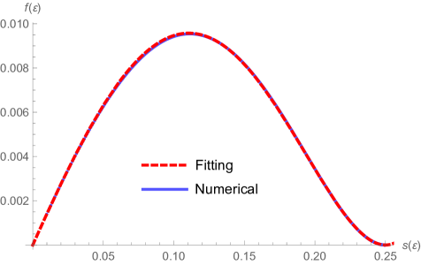
Figure 5: The contribution to $v_{B}$ from processes with overlapping OTOCs is given by $2g(\varepsilon)^{2}f(\varepsilon)/q^{2}$, $f(\varepsilon)$ is by numerically and plotted in blue. A fitting function is plotted in red.

with $s(\varepsilon)=\sin(\varepsilon)^{2}\cos(\varepsilon)^{2}$ and $\nu(\varepsilon)=[4(1-2s)(1-s(1-2s))]^{-1}$ and where $f(\varepsilon)$ is given to good approximation (Fig. 5) by

$$f(\varepsilon)=\frac{1}{7}s(\varepsilon)(1-4s(\varepsilon))^{2}(1+6.8s+16.1s^{2}).$$ (76)

It turns out that the contribution $\delta v_{S}(\varepsilon)$ only arises because of the spatial ($S$) translation symmetry of the model: the scramblers in any particular Floquet layer are identical. On the other hand, $\delta v_{F}(\varepsilon)$ arises due to both the spatial and Floquet ($F$) symmetries in the problem. To see this, we analyse variations of the model without spatial translation and Floquet symmetry (see App. E). In Fig. 2 we plot the different contributions to $\langle\delta v_{B}\rangle\equiv\langle v_{B}\rangle-v_{0}$.

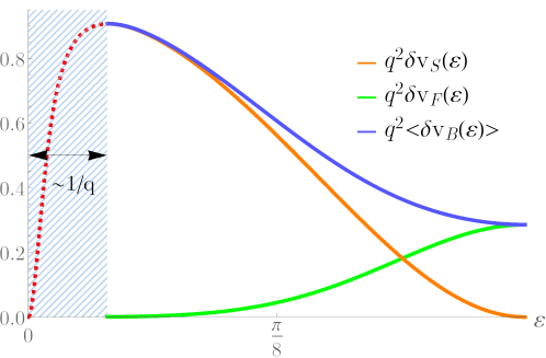
Figure 2: The contributions $\delta v_{S}(\varepsilon)$ and $\delta v_{F}(\varepsilon)$ to $\langle\delta v_{B}\rangle$. As $\varepsilon\to 0$, the perturbative expansion in $1/q$ breaks down (see Sec. 7.2). $\delta v_{B}$ must rapidly approach zero, in E.1 we argue that this happen over an $\mathcal{O}(1/q)$ window.

Spatial disorder is often associated with localization, and a suppression of transport. On the other hand the spatiotemporal randomness in random circuits promotes ergodicity, and the rapid growth of operators. Our results for $v_{B}$ are more in agreement with the former intuition – translational symmetry enhances transport – because the butterfly velocity receives an enhancement $\delta v_{S}>0$ when spatial translation symmetry is present. Even less obvious is the role of Floquet symmetry; like translational symmetry, we find an enhancement $\delta v_{F}>0$ to $v_{B}$. It will be interesting to understand whether these effects are robust at higher orders in perturbation theory, and hold for more general time evolutions.

We now briefly discuss the difficulties with small $\varepsilon$. The $\varepsilon\to 0$ limit represents an obvious sanity check on our results, but also represents a challenging limit in a memory matrix calculation. As $\varepsilon\to 0$, the memory time must diverge, limiting our ability to truncate the memory effects. This is demonstrated in the failure of Eq. 74 for $v_{B}$ to vanish for $\varepsilon=0$ where sites decouple and the butterfly velocity is zero. As the memory time reaches $t\sim q$, or equivalently once $\varepsilon\sim 1/q$, our perturbative expansion in $1/q$ breaks down. Therefore, the corrections $\langle\delta v_{B}\rangle$ as given in (74) are valid only for $\varepsilon>\mathcal{O}(1/q)$, below which $\langle\delta v_{B}\rangle$ must quickly go to zero as shown in Fig. 2. We discuss this in detail in Sec. 7.2.

6 Calculating corrections from memory effects

In this section we first present the large $q$ scaling results that form the backbone of the perturbative expansion of $\Sigma(t)$, before presenting a intricate booking keeping of the $\mathcal{O}(1/q^{2})$ contributions in Sec. 6.2.

6.1 Averaging $n$-point correlation functions and their moments

In this section we will present several useful theorems concerning the Haar averages of correlators and products of correlators with random unitary dynamics. The reader is directed to [51] for the proofs of the theorems below. We need only consider correlation functions involving $Z$’s:

$$\langle\mathcal{Z}(\bm{t})\rangle\equiv\langle Z(t_{1})\cdots Z(t_{n})\rangle=\frac{1}{q}\Tr[Z(t_{1})\cdots Z(t_{n})],$$ (77)

where $\bm{t}=\left(t_{1},\cdots,t_{n}\right)$ and $\mathcal{Z}(\bm{t})=Z(t_{1})\cdots Z(t_{n})$ is a product of $n$ ‘scrambled’ Pauli $Z$ matrices $Z(t)=V^{t}ZV^{-t}$ (with a Haar random unitary $V$). We call correlators of form Eq. 77 arbitrary-time-ordered (ATO) $n$-point correlation functions as the times $t_{i}$ are not forced to be ordered. A correlator is trivial if $\mathcal{Z}(\bm{t})=\mathbb{1}$. For the purposes of this section, we assume that none of the correlators are trivial.

Before we present the theorems, let us introduce what we call the decoration delta constraint, $\delta^{A,B}$. This is zero unless the two operators $A=Z(a_{1})\cdots Z(a_{n})$ and $B=Z(b_{1})\cdots Z(b_{n})$ are equal, $AB^{-1}=\mathbb{1}$, for all scrambling unitaries $V$. If the strings $\bm{a}=(a_{1},\cdots,a_{n})$ and $\bm{b}=(b_{1},\cdots,b_{n^{\prime}})$ do not have repeated consecutive times, then the delta constraint simply checks that $\bm{a}=\bm{b}$. Otherwise, we need to introduce a concept called the minimal form of a operator.

Definition 1 (Minimal form).

With $\mathcal{Z}(\bm{t})=Z(t_{1})\cdots Z(t_{n})$ as a product of scrambled Pauli Z operators and $\mathcal{Z}(\bm{t}^{\prime})=Z(t^{\prime}_{1})\cdots Z(t^{\prime}_{n})$ as the form reached after exhaustively using the property $Z(t)^{2}=\mathbb{1}$, we define the minimal form of $\mathcal{Z}(\bm{t})$ as $\textrm{Min}(\mathcal{Z}(\bm{t}))\equiv\mathcal{Z}(\bm{t}^{\prime})$. We also define the minimal form of the string $\bm{t}$ as $\textrm{Min}(\bm{t})\equiv\bm{t}^{\prime}$.

We can then give a more general definition of the delta constraint.

Definition 2 (Decoration delta constraint).

The delta constraint $\delta^{A,B}$ on operators $A=Z(a_{1})\cdots Z(a_{n})$ and $B=Z(b_{1})\cdots Z(b_{n})$ is defined by

$$\delta^{A,B}=\begin{cases}1,\quad\textrm{if }\textrm{Min}(\bm{a})=\textrm{Min}(\bm{b})\\ 0,\quad\textrm{otherwise}.\end{cases}$$ (78)

Theorem 1.

The Haar average of a product of $p$ ATO correlators has the following scaling behaviour,

$$\int dU\langle\mathcal{Z}(\bm{t}^{1})\rangle\cdots\langle\mathcal{Z}(\bm{t}^{p})\rangle=\mathcal{O}(1/q^{2\lfloor p/2\rfloor})\quad\textrm{as $q\to\infty$}.$$ (79)

Theorem 2.

The Haar average of a product of two ATO correlators is given by

$$\int dU\langle\mathcal{Z}(\bm{t})\rangle\langle\mathcal{Z}(\bm{t}^{\prime})\rangle^{*}=\frac{S(\bm{t})}{q^{2}}\sum_{\tau\in\mathbb{Z}}\delta^{\mathcal{Z}(\bm{t+\tau}),\mathcal{Z}(\bm{t}^{\prime})}+\mathcal{O}(1/q^{3})\quad\textrm{as $q\to\infty$},$$ (80)

where we have used the decoration delta constraint and where the sum over $\tau$ allows for $\bm{t}$ and $\bm{t}^{\prime}$ to differ by a global shift in time. The symmetry factor $S(\bm{t})$ counts the degree of cyclic symmetry of the list of times $\bm{t}$, if there exists $n$ cyclic permutations $\alpha$ such that $\alpha(\bm{t})=\bm{t}$, then $S(\bm{t})=n$.

We will often study a special subset of ATO correlators, which we dub physical OTOCs. These take the form $\langle Z\Gamma_{1}Z(T)\Gamma_{\overline{2}}^{\dagger}Z\Gamma_{2}Z(T)\Gamma_{\overline{1}}^{\dagger}\rangle$, where $\Gamma_{i}=Z(1)^{s^{i}_{1}}Z(2)^{s^{i}_{2}}\cdots Z(T-1)^{s^{i}_{T-1}}$ for binary strings $\bm{s}^{i}=(s^{i}_{1},\cdots,s^{i}_{T-1})$.

Theorem 3.

The Haar average of a physical OTOC is given by

$$\int dV\langle Z\Gamma_{1}Z(T)\Gamma_{\overline{2}}^{\dagger}Z\Gamma_{2}Z(T)\Gamma_{\overline{1}}^{\dagger}\rangle=\frac{1}{q^{2}} \left(\delta^{\Gamma_{1}\Gamma_{\overline{1}}^{\dagger}\Gamma_{2}\Gamma_{\overline{2}}^{\dagger},\mathbb{1}}-\delta^{\Gamma_{1},\Gamma_{\overline{2}}}\delta^{\Gamma_{2},\Gamma_{\overline{1}}}-\delta^{\Gamma_{1},\Gamma_{\overline{1}}}\delta^{\Gamma_{2},\Gamma_{\overline{2}}}\right)$$

$$+\mathcal{O}(1/q^{3}),$$ (81)

where we have again used the decoration delta constraint. This result relies on theorem 4 of [51] and is obtained in Eq. 138 of B.

6.2 Computing $\Sigma$ at $\mathcal{O}(1/q^{2})$

We now compute the memory matrix at leading order in $1/q$, enabling us to calculate the butterfly velocity to $\mathcal{O}(1/q^{2})$. As discussed in Sec. 3, we calculate the proxy $\sigma(k,z)$ instead of $\Sigma(k,z)$. We will find that the $\mathcal{O}(1/q^{2})$ contributions to $\sigma(k,t)$ decays exponentially fast with a decay-rate $\gamma(\varepsilon)\approx 2\lvert g(\varepsilon)\rvert$ set by the interaction strength $\varepsilon$.

It is convenient to express $\sigma(k,z)$ as

$$\sigma(k,z)=\eta(k)(1-e^{-\mathrm{i}k})\mathcal{D}(k,z),$$ (82)

where

$$\mathcal{D}(k,z)=\sum_{x}q^{x}e^{-ikx}\mathcal{D}(x,z),\quad\mathcal{D}(x,z)=q^{x}\langle F^{0}\rvert\mathcal{L}\mathcal{Q}\frac{1}{e^{-\mathrm{i}z}-1-\mathcal{L}}\mathcal{Q}\mathcal{L}\lvert F^{x}\rangle.$$ (83)

Corrections to $v_{B}$ from fast processes (i.e., processes counted by $\Sigma$) are then given by

$$\delta v=\lim_{z\to i0^{+}}\lim_{k\to 0}i\sigma(k,z)/k=-\mathcal{D}(k=0,z=0).$$ (84)

We will often work with the real time version of $\mathcal{D}$,

$$\mathcal{D}(x,T)=q^{x}\langle F^{0}\rvert\mathcal{L}\mathcal{Q}\mathcal{U}^{T-1}\mathcal{Q}\mathcal{L}\lvert F^{x}\rangle.$$ (85)

We separate the scrambling part of each Floquet layer from the two-local bricks as before; $\mathcal{U}=\mathcal{V}\mathcal{U}_{Z}$. Then a product $\mathcal{U}^{n}$ can be written $\mathcal{U}^{n}=\mathcal{U}_{Z}(1)\mathcal{U}_{Z}(2)\cdots\mathcal{U}_{Z}(n)\mathcal{V}^{n}$ where $\mathcal{U}_{Z}(t)=\mathcal{V}^{t}\mathcal{U}_{Z}\mathcal{V}^{-t}$. One consequence is that

$$\langle F^{0}\rvert\mathcal{L}=\langle F^{0}\rvert\mathcal{U}-\langle F^{0}\rvert\mathbb{1}=\langle F^{0}\rvert\mathcal{V}\mathcal{U}_{Z}-\langle F^{0}\rvert=\langle F^{0}\rvert\mathcal{L}_{Z}$$ (86)

where $\mathcal{L}_{Z}=\mathcal{U}_{Z}-\mathbb{1}$. We can similarly show $\mathcal{L}\lvert F^{x}\rangle=\mathcal{V}\mathcal{L}_{Z}\lvert F^{x}\rangle$. Using this and $\left[\mathcal{V},\mathcal{Q}\right]=0$ and simplifying the notation $\mathcal{L}_{Z}\to L$ and $\mathcal{U}_{Z}\to U$, $\mathcal{D}(x,T)$ can be written as

$$\mathcal{D}(x,T)=q^{x}\langle F^{0}\rvert L\mathcal{Q}U(1)\cdots U(T-1)\mathcal{Q}L(T)\lvert F^{x}\rangle,$$ (87)

Using the decoration expansion for each brick Eq. 67, we express $\mathcal{D}(x,T)$ as a sum over decorations $\Gamma$,

$$\mathcal{D}(x,T)=\sum_{\Gamma}C_{\Gamma}\mathcal{D}_{\Gamma}(x,T),\quad\mathcal{D}_{\Gamma}(x,T)=q^{x}\langle F^{0}\rvert L\mathcal{Q}\Gamma\mathcal{Q}L(T)\lvert F^{x}\rangle.$$ (88)

$\Gamma=\bigotimes_{r}\,\Gamma^{r}$ is a product of decorations on every site. The decoration on some site $r$ is given by $\Gamma^{r}=\Gamma^{r}_{1}\otimes\Gamma^{r*}_{\overline{1}}\otimes\Gamma^{r}_{2}\otimes\Gamma^{r*}_{\overline{2}}$ (i.e., a product of decorations on each leg of the site) and where $\Gamma^{r}_{i}=Z(1)^{s^{r,i}_{1}}Z(2)^{s^{r,i}_{2}}\cdots Z(T-1)^{s^{r,i}_{T-1}}$ for a binary string $\bm{s}^{r,i}=(s^{r,i}_{1},\cdots,s^{r,i}_{T-1})$. We will use the decoration expansion, and a carefully chosen decomposition of the initial states to express contributions as products of ATO’. We will use the theorems 1 - 3 to see what kinds of decorations can give rise to $O(1/q^{2})$ corrections to the circuit averaged $\sigma$, and then evaluate those. It turns out that only certain values of $x$ are relevant, $x=0,1,2$ at this order, as we will see.

Using the inversion symmetry of the Floquet unitary, we find

$$\mathcal{D}(-x,T)=q^{-2x}\mathcal{D}(x,T),\quad\textrm{for $x>0$}.$$ (89)

We conclude that the contributions from $x<0$ are at least a factor $1/q^{2}$ smaller than the $x>0$ contributions. In the remainder of this section we will see that the contributions for $x\geq 0$ are no larger than $\mathcal{O}(1/q^{2})$, and that therefore $\mathcal{D}(x<0,T)=\mathcal{O}(q^{-4})$. We will therefore only consider $x\geq 0$ in the following sections.

To evaluate $\mathcal{D}_{\Gamma}$, we first project $L(T)\lvert F^{x}\rangle$ onto the fast space.

$$\begin{matrix}\mathcal{Q}L(T)\lvert F^{x}\rangle=g\left[-\begin{matrix}\\ \ \end{matrix}\right.\\ \ \end{matrix}\begin{matrix}\lvert\phi_{+}(T)\rangle\\ \lvert-\rangle\\ {\color[rgb]{.5,.5,.5}\textrm{1}}\end{matrix}\begin{matrix}\ -\ \begin{matrix}\\ \ \end{matrix}\\ \ \end{matrix}\begin{matrix}\lvert+\rangle\\ \lvert\phi_{-}(T)\rangle\\ {\color[rgb]{.5,.5,.5}\textrm{2}}\end{matrix}\begin{matrix}\ +\ \begin{matrix}\\ \ \end{matrix}\\ \ \end{matrix}\begin{matrix}Z(T)^{\otimes 2}\lvert+\rangle\\ Z(T)^{\otimes 2}\lvert-\rangle\\ {\color[rgb]{.5,.5,.5}\textrm{3}}\end{matrix}\begin{matrix}\left.\begin{matrix}\\ \ \end{matrix}\right]\\ \ \end{matrix}\begin{matrix}-\mathrm{i}h\begin{matrix}\\ \ \end{matrix}\\ \ \end{matrix}\begin{matrix}K(T)\lvert+\rangle\\ K(T)\lvert-\rangle\\ {\color[rgb]{.5,.5,.5}\textrm{4}}\end{matrix}\ \ \begin{matrix}{\color[rgb]{.5,.5,.5}\textrm{site }x}\\ {\color[rgb]{.5,.5,.5}\textrm{site }x+1}\\ \ \end{matrix}$$ (90)

where we have suppressed sites $r<x$ ($r>x+1$) and carefully chosen an orthogonal decomposition of $QL(T)\lvert F^{x}\rangle$ in terms of four fast states, numbered from $1$ to $4$. We have used the shorthand $Z^{\otimes 2}$ and $K$ to represent the following,

$$\raisebox{-0.45pt}{\includegraphics[height=31.2982pt]{Diagrams2/ZtensorZ.png}},\ \raisebox{-0.45pt}{\includegraphics[height=31.2982pt]{Diagrams/Kdec.png}}.$$ (91)

$Z(T)^{\otimes 2}$ and $K(T)$ are defined identically but with $Z(T)$ in place of $Z$. Finally, $\lvert\phi_{+}(T)\rangle$ and $\lvert\phi_{-}(T)\rangle$ are given by

$$\lvert\phi_{+}(T)\rangle=Z(T)^{\otimes 2}\lvert+\rangle-\frac{1}{q-q^{-1}}\lvert\perp\rangle,\quad\lvert\phi_{-}(T)\rangle=Z(T)^{\otimes 2}\lvert-\rangle-\frac{1}{q-q^{-1}}\lvert 0\rangle,$$ (92)

where $\lvert\perp\rangle=\lvert-\rangle-\frac{1}{q}\lvert+\rangle$. The initial state is easily found using $\langle F^{0}\rvert L\mathcal{Q}=\left(\mathcal{Q}L\lvert F^{0}\rangle\right)^{T}$.

The four states numbered in Eq. 90 obey a useful set of identities, which allow us to identify and discard many lower order diagrams and significantly simplify the memory matrix calculation.

6.2.1 Identities of the $\phi_{\pm}$ states

It will be useful to determine some properties of $\lvert\phi_{+}\rangle$ and $\lvert\phi_{-}\rangle$. The isometry $S=(1\leftrightarrow 2)$ (swaps legs $1$ and $2$) relates the two vectors, $S\lvert\phi_{-}\rangle=\lvert\phi_{+}\rangle$. We can then investigate $\lvert\phi_{-}\rangle$ only. Firstly, $\lvert\phi_{-}\rangle$ has no overlap with either $\lvert+\rangle$ or $\lvert-\rangle$.

$$\langle-\rvert\lvert\phi_{-}\rangle =\langle-\rvert Z^{\otimes 2}\lvert-\rangle-\frac{1}{q-q^{-1}}\langle-\rvert\lvert 0\rangle=\langle-\rvert Z^{\otimes 2}\lvert-\rangle=\raisebox{-0.38pt}{\includegraphics[height=28.45274pt]{Diagrams/minusZminus.png}}=0$$

$$\langle+\rvert\lvert\phi_{-}\rangle =\langle+\rvert Z^{\otimes 2}\lvert-\rangle-\frac{1}{q-q^{-1}}\langle+\rvert\lvert 0\rangle=\raisebox{-0.4pt}{\includegraphics[height=31.2982pt]{Diagrams2/plusphiminus.png}}$$

$$=\frac{1}{q}-\frac{1}{q-q^{-1}}(1-q^{-2})=0.$$

Using $S$, we can then write

$$\langle\phi_{+}\rvert\lvert\pm\rangle=\langle\phi_{-}\rvert\lvert\pm\rangle=\langle\pm\rvert\lvert\phi_{+}(T)\rangle=\langle\pm\rvert\lvert\phi_{-}(T)\rangle=0.$$ (93)

We next consider what happens when the wires of $\langle\pm\rvert$ are decorated. Let $\Gamma^{r}$ be a decoration on the four legs of some site $r$, i.e., $\Gamma^{r}=\Gamma^{r}_{1}\otimes\Gamma^{r*}_{\overline{1}}\otimes\Gamma^{r}_{2}\otimes\Gamma^{r*}_{\overline{2}}$, where each $\Gamma^{r}_{i}$ take the form $\Gamma_{i}=Z(1)^{s^{i}_{1}}\cdots Z(T-1)^{s^{i}_{T-1}}$ for some bit-string $\bm{s}_{i}$. This is shown graphically below.

$$\Gamma^{r}=\raisebox{-0.45pt}{\includegraphics[height=73.97733pt]{Diagrams2/single-site-gamma.png}}.$$ (94)

The overlaps between $\lvert\phi_{-}(T)\rangle$ and a decorated $\langle+\rvert$ state is then given by

$$\langle+\rvert\Gamma^{r}\lvert\phi_{-}(T)\rangle =\raisebox{-0.45pt}{\includegraphics[height=56.9055pt]{Diagrams/NEWdoubledecplusphiminus.png}}$$

$$=\frac{1}{q}\langle Z(T)\Gamma^{r\dagger}_{\overline{2}}\Gamma^{r}_{1}Z(T)\Gamma^{r\dagger}_{\overline{1}}\Gamma^{r}_{2}\rangle$$

$$\quad\quad-\frac{1}{q-q^{-1}}\left(\langle\Gamma^{r\dagger}_{\overline{2}}\Gamma^{r}_{1}\rangle\langle\Gamma^{r\dagger}_{\overline{1}}\Gamma^{r}_{2}\rangle-\frac{1}{q^{2}}\langle\Gamma^{r\dagger}_{\overline{2}}\Gamma^{r}_{1}\Gamma^{r\dagger}_{\overline{1}}\Gamma^{r}_{2}\rangle\right).$$ (95)

Similar identities hold for the overlaps $\langle+\rvert\lvert\phi_{-}(T)\rangle$ and $\langle\phi_{-}\rvert\lvert\pm\rangle$. These identities can be summarised as follows

$$\langle-\rvert\Gamma^{r}\lvert\phi_{-}(T)\rangle =\langle Z(T)\Gamma^{r\dagger}_{\overline{1}}\Gamma^{r}_{1}\rangle\langle Z(T)\Gamma^{r\dagger}_{\overline{2}}\Gamma^{r}_{2}\rangle-\frac{1}{q^{2}-1}\left(\langle\Gamma^{r\dagger}_{\overline{1}}\Gamma^{r}_{1}\Gamma^{r\dagger}_{\overline{2}}\Gamma^{r}_{2}\rangle-\langle\Gamma^{r\dagger}_{\overline{1}}\Gamma^{r}_{1}\rangle\langle\Gamma^{r\dagger}_{\overline{2}}\Gamma^{r}_{2}\rangle\right),$$

$$\langle\phi_{-}\rvert\Gamma^{r}\lvert+\rangle =\frac{1}{q}\langle Z\Gamma^{r}_{1}\Gamma^{r\dagger}_{\overline{2}}Z(T)\Gamma^{r}_{2}\Gamma^{r\dagger}_{\overline{1}}\rangle-\frac{1}{q-q^{-1}}\left(\langle\Gamma^{r}_{1}\Gamma^{r\dagger}_{\overline{2}}\rangle\langle\Gamma^{r}_{2}\Gamma^{r\dagger}_{\overline{1}}\rangle-\frac{1}{q^{2}}\langle\Gamma^{r}_{1}\Gamma^{r\dagger}_{\overline{2}}\Gamma^{r}_{2}\Gamma^{r\dagger}_{\overline{1}}\rangle\right),$$

$$\langle\phi_{-}\rvert\Gamma^{r}\lvert-\rangle =\langle Z(T)\Gamma^{r}_{1}\Gamma^{r\dagger}_{\overline{1}}\rangle\langle Z(T)\Gamma^{r}_{2}\Gamma^{r\dagger}_{\overline{2}}\rangle-\frac{1}{q^{2}-1}\left(\langle\Gamma^{r}_{1}\Gamma^{r\dagger}_{\overline{1}}\Gamma^{r}_{2}\Gamma^{r\dagger}_{\overline{2}}\rangle-\langle\Gamma^{r}_{1}\Gamma^{r\dagger}_{\overline{1}}\rangle\langle\Gamma^{r}_{2}\Gamma^{r\dagger}_{\overline{2}}\rangle\right).$$ (96)

In general, $\Gamma^{r}$ will insert operators on each of the four legs of the input state. However, sometimes one can utilize the wirings between each of the legs to simplify the resulting expression, an example for $\langle+\rvert\Gamma^{r}$ is shown below,

$$\raisebox{-0.45pt}{\includegraphics[height=56.9055pt]{Diagrams2/undoing_decorations.png}}.$$ (97)

We say $\Gamma^{r}$ decorates the state if this simplification process cannot be used to remove all four components of $\Gamma^{r}$. In the example above we were able to remove all of the non-identity operators from the $(2,\overline{1})$ wiring but not from the $(1,\overline{2})$ wiring. Notice that in every case in Eq. 96 and in Eq. 95, if either of the wirings in the $+/-$ states carry a non-identity operator, the overlap with the $\phi_{\pm}$ states vanishes.

Assuming that the decorations non-trivially decorate both wirings of the $+/-$ states, these overlaps can be summarised as follows

$$q\langle\pm\rvert\Gamma^{r}\lvert\phi_{\mp}(T)\rangle =\textrm{OTOC}-\textrm{Corr}\times\textrm{Corr}^{\prime}+\mathcal{O}(1/q^{2})$$

$$q\langle\phi_{\pm}\rvert\Gamma^{r}\lvert\mp\rangle =\textrm{OTOC}-\textrm{Corr}\times\textrm{Corr}^{\prime}+\mathcal{O}(1/q^{2})$$

$$\langle\pm\rvert\Gamma^{r}\lvert\phi_{\pm}(T)\rangle =\textrm{Corr}\times\textrm{Corr}^{\prime}+\mathcal{O}(1/q^{2})$$

$$\langle\phi_{\pm}\rvert\Gamma^{r}\lvert\pm\rangle =\textrm{Corr}\times\textrm{Corr}^{\prime}+\mathcal{O}(1/q^{2}).$$ (98)

Where rather than give the full expressions we have simply presented the types of contributions (i.e., OTOCs, products of non-trivial correlators or terms that are manifestly $\mathcal{O}(1/q^{2})$). This is often enough to identify diagrams that contribute to $\mathcal{D}(x,T)$ at $\mathcal{O}(1/q^{3})$. In cases that require a more careful analysis we refer to Eq. 95 and Eq. 96.

These are useful identities because the diagrams contributing to the memory kernel tend to involve products of terms of this form. We will now see how, using our OTOC identities from Sec 5, this result allows us to pinpoint which diagrams are able to contribute at leading order in $\mathcal{O}(1/q^{2})$

6.2.2 $\mathcal{D}^{a,b}(x,T)$

Casting our attention back to the orthogonal decomposition of the projected vector $\mathcal{Q}L(T)\lvert F^{x}\rangle$ in Eq. 90 where labelled each of four orthogonal states from $1$ to $4$, we now use a short hand $\{\lvert 1,x,T\rangle,\cdots,\lvert 4,x,T\rangle\}$ to denote each of these states. This is also done for $\langle F^{0}\rvert L\mathcal{Q}$. Using this, we define the following quantity,

$$\mathcal{D}^{a,b}(x,T)\equiv q^{x}\langle a,0,0\rvert U(1)U(2)\cdots U(T-1)\lvert b,x,T\rangle,$$ (99)

and also the decoration expansion quantity,

$$\mathcal{D}^{a,b}_{\Gamma}(x,T)=q^{x}\langle a,0,0\rvert\Gamma\lvert b,x,T\rangle.$$ (100)

The decoration $\Gamma$ is a product of $T-1$ decoration layers, $\Gamma=\Gamma(1)\Gamma(2)\cdots\Gamma(T-1)$, one for each unitary layer $U(t)$ of Eq. 99.

In what follows, we examine $\mathcal{D}^{a,b}$ for all possible pairs $a,b$; some calculations are carried out in C and D. All contributions are $\leq\mathcal{O}(1/q^{3})$, except for the $(2,1)$ and $(4,4)$ terms as summarised in 6.3.

6.2.3 $(a,b)=(1,1),(2,2)$ are $\mathcal{O}(1/q^{3})$

The arguments used for $(a,b)=(1,1)$ are the same as used for $(2,2)$, for brevity we will only present them for $(1,1)$. We study $x>0$ and $x=0$ separately, writing $\mathcal{D}_{\Gamma}^{1,1}(x,T)$ as diagram in both cases.

• $x>0$:

  $$\mathcal{D}^{1,1}_{\Gamma}(x>0,T)=g^{2}\times\left[\ \begin{matrix}\\ \vspace{-0.7cm}\\ {\color[rgb]{.5,.5,.5}\textrm{site }0}\\ {\color[rgb]{.5,.5,.5}\textrm{site }1}\\ \\ \\ \\ \\ \end{matrix}\ \ \begin{matrix}\ \ \vdots\\ \ \ \langle\phi_{+}\rvert\\ q\langle-\rvert\\ \ \ \vdots\\ q\langle-\rvert\\ \ \ \langle-\rvert\\ \ \ \vdots\end{matrix}\ \framebox{ $\begin{matrix}\\ \\ \\ \Gamma\\ \\ \\ \\ \end{matrix}$}\ \begin{matrix}\vdots\\ \lvert+\rangle\\ \lvert+\rangle\\ \vdots\\ \lvert\phi_{+}(T)\rangle\\ \lvert-\rangle\\ \vdots\\ \end{matrix}\ \ \begin{matrix}\\ \\ \\ \\ \vspace{-0.2cm}\\ {\color[rgb]{.5,.5,.5}\textrm{site }x}\\ {\color[rgb]{.5,.5,.5}\textrm{site }x+1}\\ \\ \end{matrix}\right]$$

  Using the overlap identities Eq. 93, Eq. 95 and Eq. 96, we see that the contribution from site $0$ and $x$ either vanish or have the form

  $$\left(\textrm{Corr}_{0}\times\textrm{Corr}^{\prime}_{0}+\mathcal{O}(1/q^{2})\right)\left(\textrm{OTOC}_{x}+\textrm{Corr}_{x}\times\textrm{Corr}^{\prime}_{x}+\mathcal{O}(1/q^{2})\right).$$

  Every other site may contribute either trivial or non-trivial correlators to the product. Therefore, after Haar averaging, theorem 1 of Sec. 6.1 gives

  $$\int dV\mathcal{D}^{1,1}_{\Gamma}(x>0,T)=\mathcal{O}(1/q^{3}).$$ (101)

• $x=0$:

  $$\mathcal{D}^{1,1}_{\Gamma}(0,T)=g^{2}\times\left[\ \ {\color[rgb]{.5,.5,.5}\textrm{site }0}\ \ \begin{matrix}\ \ \vdots\\ \ \langle+\rvert\\ \langle\phi_{+}\rvert\\ \ \langle-\rvert\\ \ \ \vdots\end{matrix}\ \framebox{ $\begin{matrix}\\ \\ \Gamma\\ \\ \\ \end{matrix}$}\ \begin{matrix}\vdots\\ \lvert+\rangle\\ \lvert\phi_{+}(T)\rangle\\ \lvert-\rangle\\ \vdots\end{matrix}\right]$$

  On site $x=0$, we have

  $$\langle\phi_{+}\rvert\Gamma^{0}\lvert\phi_{+}(T)\rangle=\ \langle Z\Gamma^{0}_{1}Z(T)\Gamma^{0\dagger}_{\overline{2}}\rangle\langle Z\Gamma^{0}_{2}Z(T)\Gamma^{0\dagger}_{\overline{1}}\rangle-\frac{1}{q^{2}-1}\langle\Gamma^{0\dagger}_{\overline{1}}\Gamma^{0}_{1}Z(T)\Gamma^{0\dagger}_{\overline{2}}\Gamma^{0}_{2}Z(T)\rangle$$

  $$-\frac{1}{q^{2}-1}\langle Z\Gamma^{0}_{1}\Gamma^{0\dagger}_{\overline{1}}Z\Gamma^{0}_{2}\Gamma^{0\dagger}_{\overline{2}}\rangle+\frac{1}{q^{2}(1-q^{-2})^{2}}\langle\Gamma^{0}_{1}\Gamma^{0\dagger}_{\overline{1}}\rangle\langle\Gamma^{0}_{2}\Gamma^{0\dagger}_{\overline{2}}\rangle$$

  $$+\frac{1}{q^{2}-1}\langle Z\Gamma^{0}_{1}\Gamma^{0\dagger}_{\overline{2}}\rangle\langle Z\Gamma^{0}_{2}\Gamma^{0\dagger}_{\overline{1}}\rangle+\frac{1}{q^{2}-1}\langle\Gamma^{0\dagger}_{\overline{2}}\Gamma^{0}_{1}Z(T)\rangle\langle\Gamma^{0\dagger}_{\overline{1}}\Gamma^{0}_{2}Z(T)\rangle$$

  $$-\frac{1}{(q^{2}-1)^{2}}\langle\Gamma^{0}_{1}\Gamma^{0\dagger}_{\overline{1}}\Gamma^{0}_{2}\Gamma^{0\dagger}_{\overline{2}}\rangle-\frac{1}{(q^{2}-1)^{2}}\langle\Gamma^{0}_{1}\Gamma^{0\dagger}_{\overline{2}}\Gamma^{0}_{2}\Gamma^{0\dagger}_{\overline{1}}\rangle$$

  $$+\frac{1}{(q^{2}-1)^{2}}\langle\Gamma^{0}_{1}\Gamma^{0\dagger}_{\overline{2}}\rangle\langle\Gamma^{0}_{2}\Gamma^{0\dagger}_{\overline{1}}\rangle.$$ (102)

  The final three terms are manifestly $\mathcal{O}(1/q^{4})$. The fifth and sixth terms are of the form $\textrm{Corr}\times\textrm{Corr}^{\prime}/q^{2}$, where these correlators are non-trivial. Therefore, using theorem 1, the Haar average of these terms (possibly multiplied by additional non-trivial correlators from other sites) is $\mathcal{O}(1/q^{4})$. The second, third and fourth terms all have pre-factors of $1/q^{2}$; if they are to contribute at this order, the accompanying correlators must be trivial. Using decoration delta constraints, this fact (a consequence of theorem 1) is written below

  $$\int dV\frac{1}{q^{2}}\langle\mathcal{Z}_{1}\rangle\cdots\langle\mathcal{Z}_{m}\rangle=\frac{1}{q^{2}}\prod_{i}\delta^{\mathcal{Z}_{i},\mathbb{1}}+\mathcal{O}(1/q^{3}).$$ (103)

  All together, in the context of a Haar average, the following replacement is valid up to $\mathcal{O}(1/q^{2})$.

  $$\langle\phi_{+}\rvert\Gamma^{0}\lvert\phi_{+}(T)\rangle=\langle Z\Gamma^{0}_{1}Z(T)\Gamma^{0\dagger}_{\overline{2}}\rangle\langle Z\Gamma^{0}_{2}Z(T)\Gamma^{0\dagger}_{\overline{1}}\rangle-\frac{1}{q^{2}}\delta^{\Gamma^{0}_{\overline{1}},\Gamma^{0}_{1}}\delta^{\Gamma^{0}_{\overline{2}},\Gamma^{0}_{2}}+\mathcal{O}(1/q^{3}).$$ (104)

  We say that a decoration $\Gamma^{r}$ leaves a site $r$ undecorated if it contributes only trivial correlators, $\langle\mathbb{1}\rangle$ . In the present case Keeping only $\mathcal{O}(1/q^{2})$ contributions forces all sites $r\neq 0$ to be left undecorated. This allows us to take the Haar average of Eq. 104 directly, using theorem 2 for the Haar average of a product of two correlators. This gives,

  $$\int dV\langle\phi_{+}\rvert\Gamma^{0}\lvert\phi_{+}(T)\rangle=\frac{1}{q^{2}}\delta^{\Gamma^{0}_{\overline{1}},\Gamma^{0}_{1}}\delta^{\Gamma^{0}_{\overline{2}},\Gamma^{0}_{2}}-\frac{1}{q^{2}}\delta^{\Gamma^{0}_{\overline{1}},\Gamma^{0}_{1}}\delta^{\Gamma^{0}_{\overline{2}},\Gamma^{0}_{2}}+\mathcal{O}(1/q^{3})=\mathcal{O}(1/q^{3}).$$ (105)

The analysis of $x<0$ would replicate that of $x>0$, but with an additional factor of $q^{-2\lvert x\rvert}$. The for all $x$, $\int dV\mathcal{D}^{1,1}_{\Gamma}(x,T)=\mathcal{O}(1/q^{3})$. Alternatively,

$$\int dV\mathcal{D}^{1,1}(k,T)=\mathcal{O}(1/q^{3}).$$ (106)

6.2.4 $(a,b)=(4,4)$ is $\mathcal{O}(1/q^{2})$

The (4,4) calculation is significantly more difficult; we present the full calculation here, however; readers interested only in the final result should skip to the summary in Sec. 6.3.

We use the decoration expansion once again to rule out contributions from $x>0$ and to identify the relevant contributions from $x=0$.

• $x>0$:

  $$\mathcal{D}^{4,4}_{\Gamma}(x>0,T)=-h^{2}\times\left[\ \begin{matrix}\vspace{-4pt}\\ {\color[rgb]{.5,.5,.5}\textrm{site }0}\\ {\color[rgb]{.5,.5,.5}\textrm{site }1}\\ \\ \\ \\ \\ \end{matrix}\ \ \begin{matrix}\ \ \vdots\\ \ \ \langle+\rvert K\\ q\langle-\rvert K\\ \ \ \vdots\\ q\langle-\rvert\\ \ \ \langle-\rvert\\ \ \ \vdots\end{matrix}\ \ \framebox{ $\begin{matrix}\\ \\ \\ \Gamma\\ \\ \\ \\ \end{matrix}$}\ \ \begin{matrix}\vdots\\ \lvert+\rangle\\ \lvert+\rangle\\ \vdots\\ K(T)\lvert+\rangle\\ K(T)\lvert-\rangle\\ \vdots\end{matrix}\ \ \begin{matrix}\vspace{5pt}\\ \\ \\ \\ {\color[rgb]{.5,.5,.5}\textrm{site }x}\\ {\color[rgb]{.5,.5,.5}\textrm{site }x+1}\\ \ \end{matrix}\right]$$

  For $x>1$, each of the sites $0$, $1$, $x$ and $x+1$ contribute non-trivial correlators. When $x=1$, sites $0$, $1$ and $2$ all contribute non-trivial correlators. In either case, theorem 1 gives

  $$\int dV\mathcal{D}^{4,4}_{\Gamma}(x>0,T)=\mathcal{O}(1/q^{3}).$$ (107)

• $x=0$:

  $$\mathcal{D}^{4,4}_{\Gamma}(x=0,T)=-h^{2}\times\left[\ \begin{matrix}{\color[rgb]{.5,.5,.5}\textrm{site }0}\\ {\color[rgb]{.5,.5,.5}\textrm{site }1}\\ \end{matrix}\ \ \begin{matrix}\ \ \ \ \vdots\\ \ \ \ \langle+\rvert\\ \langle+\rvert K\\ \langle-\rvert K\\ \ \ \ \langle-\rvert\\ \ \ \ \ \vdots\end{matrix}\ \framebox{ $\begin{matrix}\\ \\ \Gamma\\ \\ \\ \end{matrix}$}\ \begin{matrix}\vdots\\ \lvert+\rangle\\ K(T)\lvert+\rangle\\ K(T)\lvert-\rangle\\ \lvert-\rangle\\ \vdots\end{matrix}\right]$$

  Both sites $0$ and $1$ contribute non-trivial correlators. Keeping only the $\mathcal{O}(1/q^{2})$ contributions means selecting decorations on sites $r\neq 0,1$ that give trivial correlators only. For $r>1$ this means selecting decorations such that $\langle-\rvert\Gamma^{r}\lvert-\rangle=\langle\Gamma^{r}_{1}\Gamma^{r\dagger}_{\overline{1}}\rangle\langle\Gamma^{r}_{2}\Gamma^{r\dagger}_{\overline{2}}\rangle=\langle\mathbb{1}\rangle^{2}$ (for $r<0$ simply switch $-\leftrightarrow+$ and $1\leftrightarrow 2$ in these equations). Choosing only $\Gamma^{r}$ that leave a site $r<0$ ($r>1$) undecorated (contributing only trivial correlators) is equivalent to the decoration delta constraint $\delta^{\Gamma^{r}_{1},\Gamma^{r}_{\overline{2}}}\delta^{\Gamma^{r}_{2},\Gamma_{\overline{1}}}$ ($\delta^{\Gamma^{r}_{1},\Gamma^{r}_{\overline{1}}}\delta^{\Gamma^{r}_{2},\Gamma_{\overline{2}}}$). The implementation of these decoration delta constraints is discussed in B. The result of which is that for sites $r<0$ we sandwiching each decoration layer $\Gamma(t)$ by $\langle+\rvert$ and $\lvert+\rangle$ and by $\langle-\rvert$ and $\lvert-\rangle$ for sites $r<0$.

  Writing the definition of $K$ in Eq. 91 as $K=Z_{1}-Z_{2}$, where the index refers to which leg the $Z$ decorates, we write the following,

  $$\begin{matrix}\langle+\rvert K\Gamma^{0}K(T)\lvert+\rangle\\ \langle-\rvert K\Gamma^{1}K(T)\lvert-\rangle\end{matrix}=\sum_{i,j\in\{1,2\}}\begin{matrix}\langle+\rvert Z_{i}\Gamma^{0}Z(T)_{i}\lvert+\rangle\\ \langle-\rvert Z_{j}\Gamma^{1}Z(T)_{j}\lvert-\rangle\end{matrix}+\begin{matrix}\textrm{ terms with more than two}\\ \textrm{ non-trivial correlators}.\end{matrix}$$ (108)

  Because we are selecting only decorations which leave sites $r\neq 0,1$ undecorated, we are able to take the Haar average of this expression in isolation. Terms with more than two non-trivial correlators are $\mathcal{O}(1/q^{3})$ or smaller and are therefore discarded, leaving only the Haar average of the first term. Using theorem 2, this is given by

  $$\int dV\sum_{i,j\in\{1,2\}}\begin{matrix}\langle+\rvert Z_{i}\Gamma^{0}Z(T)_{i}\lvert+\rangle\\ \langle-\rvert Z_{j}\Gamma^{1}Z(T)_{j}\lvert-\rangle\end{matrix}=\begin{matrix}\\ \frac{1}{q^{2}}\delta^{\Gamma^{0}_{1},\Gamma^{1}_{\overline{1}}}\delta^{\Gamma^{0}_{\overline{2}},\Gamma^{1}_{1}}\delta^{\Gamma^{0}_{2},\Gamma^{0}_{\overline{1}}}\delta^{\Gamma^{1}_{2},\Gamma^{1}_{\overline{2}}}+\frac{1}{q^{2}}\delta^{\Gamma^{0}_{1},\Gamma^{1}_{\overline{2}}}\delta^{\Gamma^{0}_{\overline{2}},\Gamma^{1}_{2}}\delta^{\Gamma^{0}_{2},\Gamma^{0}_{\overline{1}}}\delta^{\Gamma^{1}_{1},\Gamma^{1}_{\overline{1}}}\\ +\left(1\leftrightarrow 2\right)+\mathcal{O}(1/q^{3}).\end{matrix}$$ (109)

  These delta constraints are implemented by sandwiching the decoration layers $\Gamma(t)$ with the appropriate wirings. The four different wirings configurations for sites $0$ and $1$ are shown below.

  .

  Counting only the relevant decorations $\Gamma$, $\mathcal{D}^{1,1}_{\Gamma}(x=0,T)$ given by

  $$\int dV\mathcal{D}^{4,4}_{\Gamma}(x=0,T)=-\frac{h^{2}}{q^{2}}\sum_{i,j\in\{1,2\}}\raisebox{-0.47pt}{\includegraphics[height=108.12054pt]{Diagrams/decoration_layer_rewiring.png}}$$ (110)

  We now sum over all decorations $\Gamma$ weighted by the coefficients $C_{\Gamma}$ appearing in Eq. 88. This converts back into the picture with full unitary layers $U(t)$. Using the property Eq. 70 for 2-local bricks contracted with the states $\langle\pm\rvert\otimes\langle\pm\rvert$ or $\lvert\pm\rangle\otimes\lvert\pm\rangle$, $\int dV\mathcal{D}^{1,1}(x=0,T)$ is given by the simplified form

  $$\int dV\mathcal{D}^{4,4}(x=0,T) =-\frac{h^{2}}{q^{2}}\sum_{i,j}\raisebox{-0.45pt}{\includegraphics[height=56.9055pt]{Diagrams/44-projector-insertion.png}}+\mathcal{O}(1/q^{3})$$

  $$=-\frac{h^{2}}{q^{2}}\sum_{i,j}\langle\mathcal{C}_{i,\overline{j}}\rvert\mathcal{T}\lvert\mathcal{C}_{i,\overline{j}}\rangle^{n}+\mathcal{O}(1/q^{3}),$$ (111)

  where $\mathcal{T}$ is given by

  $$\raisebox{-0.45pt}{\includegraphics[height=51.21504pt]{Diagrams/Caligraphic_T.png}},$$ (112)

  and where the tensor contractions $T_{+}$ and $T_{-}$ are given algebraically by

  $$\raisebox{-0.3pt}{\includegraphics[height=27.5992pt]{Diagrams2/Tplus_def.png}},\ \raisebox{-0.31pt}{\includegraphics[height=24.18501pt]{Diagrams2/Tminus_def.png}}$$ (113)

  Due to the replica symmetry of the unitary evolution operator, $(1,\overline{1})\leftrightarrow(2,\overline{2})$, the contributions from the $(i,j)=(1,1)$ and $(2,2)$ wirings are identical, as are $(1,2)$ and $(2,1)$ wirings. The unitary $e^{-\mathrm{i}\varepsilon\mathcal{L}}$ also has the property $\textrm{Sw}(1,\overline{1})\textrm{Sw}(2,\overline{2})e^{-\mathrm{i}\varepsilon\mathcal{L}}\textrm{Sw}(1,\overline{1})\textrm{Sw}(2,\overline{2})=(e^{-\mathrm{i}\varepsilon\mathcal{L}})^{*}$, where $\textrm{Sw}(i,\overline{i})$ swaps unbarred leg $i$ and barred leg $\overline{i}$. This transformation is a symmetry of the $\langle+\rvert$ and $\langle-\rvert$ wirings while exchanging the $\mathcal{C}_{1,\overline{1}}$ ($\mathcal{C}_{2,\overline{2}}$) and $\mathcal{C}_{2,\overline{1}}$ ($\mathcal{C}_{1,\overline{2}}$) wirings. Therefore,

  $$\xi(\varepsilon)\equiv\langle\mathcal{C}_{1,\overline{1}}\rvert\mathcal{T}\lvert\mathcal{C}_{1,\overline{1}}\rangle=\langle\mathcal{C}_{2,\overline{2}}\rvert\mathcal{T}\lvert\mathcal{C}_{2,\overline{2}}\rangle=\langle\mathcal{C}_{1,\overline{2}}\rvert\mathcal{T}\lvert\mathcal{C}_{1,\overline{2}}\rangle^{*}=\langle\mathcal{C}_{2,\overline{1}}\rvert\mathcal{T}\lvert\mathcal{C}_{2,\overline{1}}\rangle^{*}.$$ (114)

  Using the decoration decomposition of a brick in Eq. 67 and the expressions for $T_{+}$ and $T_{-}$ in Eq. 113, $\xi(\varepsilon)$ is found to be

  $$\xi(\varepsilon)=(1+g)^{2}-2\mathrm{i}hg.$$ (115)

  All together we find,

  $$\int dV\mathcal{D}^{4,4}(x=0,T)=-\frac{4h^{2}}{q^{2}}\Re\{\xi^{T-1}\}+\mathcal{O}(1/q^{3}).$$ (116)

Summing over $x$, we find the $\mathcal{O}(1/q^{2})$ contribution to $\int dV\mathcal{D}^{4,4}(k,T)$ is given by precisely the same quantity. The decay rate is given by $\gamma(\varepsilon)\equiv\ln(\lvert\xi\rvert^{-1})$, which is always close to $2\lvert g(\varepsilon)\rvert$, $2\lvert g(\varepsilon)\rvert\leq\gamma(\varepsilon)\leq 4\ln(2)\lvert g(\varepsilon)\rvert$.

6.3 Table of results and summary

We summarise the contributions $\int dV\mathcal{D}^{a,b}(k=0,T)$ in the table below, highlighting the only contributions at $\mathcal{O}(1/q^{2})$.

$a$ $\backslash$  $b$	$1$	$2$	$3$	$4$
$1$	$q^{-3}$	$q^{-3}$	$q^{-3}$	$q^{-3}$
$2$	$q^{-2}$	$q^{-3}$	$q^{-3}$	$q^{-3}$
$3$	$q^{-3}$	$q^{-3}$	$q^{-3}$	$q^{-3}$
$4$	$q^{-3}$	$q^{-3}$	$q^{-3}$	$q^{-2}$

We calculate the $(a,b)=(2,1)$ contribution in C, and in D we find that the remaining pairs $(a,b)$ contribute at $\mathcal{O}(1/q^{3})$ or smaller. Using Eq. 84, we are only required to know $\int dV\mathcal{D}^{a,b}(k=0,z=0)$ to determine the butterfly velocity. For $(4,4)$ this is given below, with the re-parameterisation $s(\varepsilon)=\sin(\varepsilon)^{2}\cos(\varepsilon)^{2}$,

$$\int dV\mathcal{D}^{(4,4)}(k=0,z=0)=-\frac{1}{q^{2}}\frac{1+5s-4s^{2}}{1-s-3s^{2}}+\mathcal{O}(1/q^{3}).$$ (117)

This re-parameterisation is motivated by the following observations about the dependence of $v_{B}$ and $D$ on $\varepsilon$. Firstly, under the variable shift $\varepsilon\to\pi/2+\varepsilon$, the full coupling unitary then transforms as $e^{-\mathrm{i}\varepsilon H}\to(-\mathrm{i})^{N-1}e^{-\mathrm{i}\varepsilon H}$. The operator dynamics is blind to global phases, meaning that $\varepsilon\to\pi/2+\varepsilon$ is a symmetry of $v_{B}(\varepsilon)$ and $D(\varepsilon)$. Secondly, by globally swapping leg $1$ with $\overline{1}$ and $2$ with $\overline{2}$, we find $\Sigma_{V,\varepsilon}(k,z)=\Sigma_{V^{*},-\varepsilon}(k,z)$. and $\Omega_{\varepsilon}(k)=\Omega_{-\varepsilon}(k)$, where we have have labelled $\Sigma$ with the scrambler and coupling strength and labelled $\Omega$ with the coupling strength used ($\Omega$ is independent of $V$). By integrating over $V$, we find another symmetry of the circuit averaged butterfly velocity and diffusion constant $\langle v_{B}(\varepsilon)\rangle$ and $\langle D(\varepsilon)\rangle$, namely $\varepsilon\to-\varepsilon$. Using these symmetries, we determine that $\langle v_{B}\rangle$ is a function of $s(\varepsilon)$ only.

For $(a,b)=(2,1)$, we find

$$\int dV\mathcal{D}^{(2,1)}(k=0,z=0)=\frac{2g^{2}}{q^{2}}(f(\varepsilon)-\nu(\varepsilon))+\mathcal{O}(1/q^{3}).$$ (118)

where $\nu(\varepsilon)=[4(1-2s)(1-s(1-2s))]^{-1}$ and where $f(\varepsilon)$ is found by numerically evaluating a sum involving a $5\times 5$ transfer matrix in C and given to good approximation (Fig. 5) by

$$f(\varepsilon)=\frac{1}{7}s(\varepsilon)(1-4s(\varepsilon))^{2}(1+as+bs^{2})$$ (119)

where $a=6.8$ and $b=16.1$. The factors $\frac{1}{7}s(1-4s)^{2}$ is obtained analytically by diagonalising the transfer matrix at small $s$ and around the point $s=1/4$. Altogether, we then find

$$\int dV\mathcal{D}(k=0,z=0)=2\frac{g^{2}}{q^{2}}(f(\varepsilon)-\nu(\varepsilon))-\frac{1}{q^{2}}\frac{1+5s-4s^{2}}{1-s-3s^{2}}+\mathcal{O}(1/q^{3}).$$ (120)

so that the correction to the circuit averaged butterfly velocity is

$$\langle\delta v_{B}(\varepsilon)\rangle=-\int dV\mathcal{D}(k=0,z=0)=\delta v_{F}(\varepsilon)+\delta v_{S}(\varepsilon)+\mathcal{O}(1/q^{3}),$$ (121)

where

$$\delta v_{F}(\varepsilon)=2\frac{g^{2}}{q^{2}}(\nu(\varepsilon)-f(\varepsilon)),\quad\delta v_{S}(\varepsilon)=\frac{1}{q^{2}}\frac{1+5s-4s^{2}}{1-s-3s^{2}}.$$ (122)

As discussed in Sec. 5, the correction $\delta v_{S}(\varepsilon)$ only arises because of the spatial translation symmetry of the model. Whereas $\delta v_{F}(\varepsilon)$ arises due to both the spatial and Floquet symmetries. To illustrate this point, we carry out a similar calculation for a version of the model with independently distributed scramblers $V_{x,t}$ for each site $x$ and at each layer of unitaries $U_{t}$. This is done in E where we find the corrections to the circuit averaged butterfly velocity $\langle\delta v\rangle\sim\mathcal{O}(1/q^{3})$, i.e., $v_{S,F}$ both vanish. Turning to the variant of the model with spatial translation symmetry but no time translation symmetry, we find $\langle\delta v_{B}\rangle=\delta v_{S}(\varepsilon)+\mathcal{O}(1/q^{3})$. Comparing these result to Eq. 74 allows us to identify the corrections to $v_{B}$ with the symmetries of the model.

Away from the weak coupling limit, the averaged butterfly velocity is given by Eq. 74. The weak coupling limit is discussed in section 7.2.

7 Discussion

In this section we discuss the late time behaviour of the memory function, addressing the limitations of the Haar averaged ATO’ results of Sec. 6.1. We also discuss the break down of the perturbative scheme used in Sec. 6.2 as $\varepsilon\to 0$.

7.1 Late times

We have presented a Kubo-like formula for $v_{B}$ in Eq. 61, involving the time integral of a correlator of fast operators, analogous to the $J$-$J$ correlation functions in Kubo formulae for more conventional transport. For $\varepsilon>0$ (more precisely $g(\varepsilon)\neq 0$), we find that the leading order correlation functions decay exponentially in time at leading order in $1/q$. Given that the correlation functions are between fast variables, it is plausible that this exponential decay is not simply an artifact of the large $q$ limit, i.e., the correlation functions decay over some time scale which is bounded below by a $q$-independent quantity $\tau(\varepsilon)$, which is positive except at exceptional point where the sites decouple i.e., when $\varepsilon=n\pi/2$ (we discuss the decoupling limit later). Assuming that $t_{\varepsilon}(q)$ is a (cutoff) time up to which we can safely use the large $q$ correlator theorems of Sec. 6.1 to identify the $\mathcal{O}(1/q^{2})$ contributions to $\Sigma$, the error incurred by truncating the infinite time evolution is $\mathcal{O}(\exp[-t_{\varepsilon}(q)/\tau(\varepsilon)])$. We will now argue that $t_{\varepsilon}(q)$ increases linearly with $q$. As a result, the error due to truncation decays exponentially in $q$, which is much smaller than the $\mathcal{O}(1/q^{2})$ corrections we calculate. This demonstrates the validity of our expansion in $q^{-1}$.

We now give some justification for the existence of a cutoff $t_{\varepsilon}(q)=cq$ for a $q$-independent constant $c$. We do this in two parts: (1) we argue that the expressions in Sec. 6.1 for the Haar average of few correlators are valid for times $t<cq$; (2) we argue that this is enough to guarantee that contributions involving many correlators (more than two) are $\mathcal{O}(1/q^{3})$ (for times $t<cq$).

In order to do this, we must go beyond the $q\to\infty$ scaling results of Sec. 6.1. In the absence of an analytical understanding of the corrections at finite $q$, we took a numerically Haar average of an assortment of ATO correlators and products of correlators, finding good evidence that the expression for the Haar average of a product of two correlators (theorem 2) and of OTOCs (theorem 3) experience only $\mathcal{O}(1/q^{3})$ errors for times $t<cq$. It turns out that this, along with the use of a Holder’s inequality and the monotonicity of the $p$-norm, is enough to bound the Haar average of arbitrarily many correlators as $\mathcal{O}(1/q^{3})$.

To show this, we start by bound the expectation of a product of many (more than two) non-trivial correlators as shown below,

$$\lvert\int dV\prod_{i}\langle\mathcal{Z}(\bm{t}_{i})\rangle\rvert\leq\int dV\prod_{i}\lvert\langle\mathcal{Z}(\bm{t}_{i})\rangle\rvert.$$ (123)

Then, using the fact $\lvert\langle\mathcal{Z}(\bm{t}_{i})\rangle\rvert\leq 1$, we can bound the average of a product of many correlators by an average over only a few. We choose to highlight three correlators

$$\lvert\int dV\prod_{i}\langle\mathcal{Z}(\bm{t}_{i})\rangle\rvert\leq\int dV\lvert\langle\mathcal{Z}(\bm{t}_{1})\rangle\rvert\lvert\langle\mathcal{Z}(\bm{t}_{2})\rangle\rvert\lvert\langle\mathcal{Z}(\bm{t}_{3})\rangle\rvert.$$ (124)

Using a generalised Holder’s inequality and monotonicity of the $p$-norm, we further bound Eq. 124 by

$$\lvert\int dV\prod_{i}\langle\mathcal{Z}(\bm{t}_{i})\rangle\rvert\leq\sqrt{\int dV\lvert\langle\mathcal{Z}(\bm{t}_{1})\rangle\rvert^{2}\int dV\lvert\langle\mathcal{Z}(\bm{t}_{2})\rangle\rvert^{2}\int dV\lvert\langle\mathcal{Z}(\bm{t}_{3})\rangle\rvert^{2}}.$$ (125)

Then, for times $t<cq$ and using theorem 2 for the second moment of a correlator, this bound takes the form

$$\lvert\int dV\prod_{i}\langle\mathcal{Z}(\bm{t}_{i})\rangle\rvert\leq C\frac{S(\bm{t}_{1})S(\bm{t}_{2})S(\bm{t}_{3})}{q^{3}},$$ (126)

for an $\mathcal{O}(1)$ constant $C$. The correlators contributing to $\Sigma$ have $1\leq S(\bm{t})\leq 2$, so that the right hand-side of Eq. 126 then simplifies to $C^{\prime}/q^{3}$ for an $\mathcal{O}(1)$ constant $C^{\prime}$. For times $t<cq$, any contribution to $\Sigma$ with three of more non-trivial correlators is $\mathcal{O}(1/q^{3})$, and the $\mathcal{O}(1/q^{2})$ contributions are counted precisely as we have done in Sec. 6.2 and the C.

7.2 The $\varepsilon\to 0$ limit

In the $\varepsilon\to 0$ limit, the Floquet unitary is given by a product of single-site unitaries, so that there is no operator growth dynamics at all ($v_{B}=0$). However, the $\varepsilon\to 0$ limit of the expression Eq. 74 yields $v_{B}=1/q^{2}$. The reason for this failure to predict the correct operator dynamics as $\varepsilon\to 0$ lies in the fact that our $1/q$ perturbative scheme breaks down once $\varepsilon$ is as small as $\varepsilon\sim 1/q$. Diagrams that we previously dismissed as $\mathcal{O}(1/q^{3})$ at strong coupling, can in fact contribute at $\mathcal{O}(1/q^{2})$ due to appearance of factors of $\varepsilon\sim 1/q$ in the denominator (after summing over time).

We do not have access to the exact expressions for the Haar average of ATO correlators in the Floquet model, instead relying on $\mathcal{O}(1/q^{2})$ results. However, in E, we study a variant of the model with independently distributed scramblers $V_{t}$ between time-step for which exact Haar averaged results are possible for certain diagrams. If we were to naively identify the $1/q^{2}$ contributions before taking a sum over time, as we did in Sec. 6.2, we would find the same, incorrect $(a,b)=(4,4)$ contribution and incorrect behaviour of $v_{B}$ as $\varepsilon\to 0$. In E.1, we consider the same family of diagrams, those involving only two non-trivial correlators (whose contribution we dub $\mathcal{D}^{4,4}_{2}$), but now take the Haar average exactly. In doing so, we find that the previously troublesome $(4,4)$ contribution now vanishes as $\varepsilon\to 0$ Eq. 223,

$$\langle\mathcal{D}^{4,4}_{2}(k=0,z=0)\rangle\approx-\frac{8\varepsilon^{2}}{1+8q^{2}\varepsilon^{2}}.$$ (127)

We suggest then, that there is a region of width $\mathcal{O}(1/q)$ in Fig. 2, where $v_{B}$ rapidly approaches zero.

8 Conclusion

In this paper, we re-purposed a hydrodynamic formalism (the memory matrix formalism) for information transport calculations by identifying the conservation of the right density of a Heisenberg time evolved operator as a pseudo-local conservation law. A number of modifications to the existing MMF are necessary: in particular, we are led to use an unusual inner product on our space of observables Eq. 20, which leads to the prediction of ballistic operator growth assuming we have identified a sufficiently complete space of slow operators. We use this new formalism to produce a Kubo formula for the butterfly velocity Eq. 36 and also find symmetry constraints on the operator growth light-cone (remark Remark).

In section 4 we used this formalism to investigate a family of translationally invariant Floquet models, finding leading order expressions for the circuit averaged butterfly velocity $v_{B}$ and operator front diffusion constant $D$. By leveraging large $q$ random unitary dynamics [51], we found that a simple hierarchy of contributions to the averaged memory matrix $\langle\Sigma\rangle$ emerges, organised by the number of non-trivial correlators contributed. This enabled us to select only the $\mathcal{O}(1/q^{2})$ contributions, associated with processes that explore a manageable sub-region of $\mathcal{Q}$ in which only the sites directly either side of the cut (the $+/-$ domain wall) are decorated by non-identity operators. We have then counted all these processes and found that at $\mathcal{O}(1/q^{2})$, the memory matrix decays exponentially fast, with an $\mathcal{O}(1)$ decay rate. We used this to calculate corrections to $v_{B}$, and were able to distinguish the effects of spatiotemporal symmetry on information transport by identifying which processes arise as a consequence of spatial translation and Floquet symmetry.

9 Further work/outlook

More exotic information hydrodynamics than biased diffusion is possible in the presence of additional conserved charges. With a U$(1)$ charge, the diffusive conserved components acts as a source of non-conserved operators, giving rise to power-law tails in the spatial distributions of operator weight [21, 22]. It will be interesting to incorporate additional symmetries, such as a U$(1)$ or fracton symmetry, into the MMF and perform a mode coupling analysis to confirm and perhaps extend existing results. Even in the presence of conservation laws, the diffusive broadening of the operator front appears ubiquitous in chaotic and interacting integrable systems in 1D [15, 52]. What makes this diffusive broadening so universal? Perhaps, by examining MMF expressions for the front diffusion constant, we can say something about the nature or number of additional slows required to find a hydrodynamical equation other than biased diffusion. Other avenues to explore include the formulation of an information mode MMF at finite temperature/chemical potential and, with only minor modifications, calculating purity. Another potentially fruitful application of formalism is in the setting of perturbed dual unitary circuits, which may serve as a testing ground for perturbative MMF calculations.

10 Acknowledgements

EM is supported by EPSRC studentship. C.v.K. is supported by a UKRI Future Leaders Fellowship MR/T040947/1.

11 References

Appendix A An unusual inner-product

In this appendix we prove that the inner-product $\left(\cdot|\cdot\right)$ defined in Eq. 20 satisfies the necessary axioms. We repeat the definition below,

$$\left(A|B\right)\equiv\langle\Phi\left(A\right)\rvert\lvert B\rangle_{\mathcal{W}}=\Tr\left(\Phi\left(A\right)^{\dagger}B\right),$$ (128)

where the super-operator $\Phi$ is given by

$$\Phi\equiv\sum_{x}\frac{1}{\chi_{x}^{2}}\lvert W^{x}\rangle\langle W^{x}\rvert+Q,\quad\chi_{x}\equiv\langle W^{x}\rvert\lvert W^{x}\rangle,\implies\Phi\lvert W^{x}\rangle=\frac{1}{\chi_{x}}\lvert W^{x}\rangle.$$ (129)

$Q$ is the Hermitian projector onto $\mathcal{Q}$. We must show that this constitutes a bona fide inner product by checking each of the inner product axioms.

1. Conjugate symmetry: $\left(A|B\right)^{*}=\left(B|A\right)$,

   Exploiting the conjugate symmetry of the inner product $\langle\cdot\rvert\lvert\cdot\rangle$, we write

   $$\left(A|B\right)=\langle\Phi\left(A\right)\rvert\lvert B\rangle=\langle A\rvert\lvert\Phi\left(B\right)\rangle=\langle\Phi\left(B\right)\rvert\lvert A\rangle^{*}=\left(B|A\right)^{*}$$ (130)

   where we have used the fact that $\Phi$ is Hermitian, this is because $\chi_{x}$ is real and the projector $\hat{Q}$ is Hermitian.

2. Linearity in second argument: $\left(A|\beta B+\gamma C\right)=\beta\left(A|B\right)+\gamma\left(A|C\right)$ for scalars $\beta,\gamma$,

   $$\left(A|\beta B+\gamma C\right) =\langle\Phi\left(A\right)\rvert\lvert\beta B+\gamma C\rangle=\beta\langle\Phi\left(A\right)\rvert\lvert B\rangle+\gamma\langle\Phi\left(A\right)\rvert\lvert C\rangle$$

   $$=\beta\left(A|B\right)+\gamma\left(A|C\right)$$ (131)

   where we have used linearity in the second argument of the inner product $\langle\cdot\rvert\lvert\cdot\rangle$.

3. Positive definiteness: $\left(A|A\right)>0$ for $A\neq 0$,

   $$\left(A|A\right)=\langle\Phi\left(A\right)\rvert\lvert A\rangle=\langle A\rvert\Phi\lvert A\rangle>0$$ (132)

   where we have used the fact that $\Phi$ is a positive definite matrix. This is easily seen by noticing that all $\chi^{2}_{x}$ are real and positive.

This confirms that $\left(A|B\right)$ is indeed an inner-product and allows us to consider a new inner-product space in which the weight operators are orthonormal.

Appendix B Imposing the decorations delta constraints

In this section we revisit the Haar average identities for ATO correlators and their moments, specifically theorems 2 and 3. The final results (at leading order in $1/q$) involved ”delta constraints” (as defined in Def. 2) which are zero/one depending on whether or not the decorations were equal (for all scramblers $V$). We have also seen these delta constraints whenever we have demanded that a correlator be trivial (see Eq. 104). In this section, we show how these delta constraints can be imposed by placing the decorations on a contour and inserting projectors at every time step; the insertion of projectors has an appealingly simple graphical interpretation, which facilitates our calculation of $\sigma$ in the main text.

B.1 The constraint $\delta^{\Gamma_{1},\Gamma_{\overline{1}}}$

The simplest example of a decoration delta constraint to consider is $\delta^{\Gamma_{1},\Gamma_{\overline{1}}}$, where the two decorations are time-ordered, i.e., $\Gamma_{1}=Z(1)^{a_{1}}Z(2)^{a_{2}}\cdots Z(n)^{a_{n}}$ and $\Gamma_{\overline{1}}=Z(1)^{b_{1}}Z(2)^{b_{2}}\cdots Z(n)^{b_{n}}$ for binary strings $\bm{a}$ and $\bm{b}$. In this case, the delta constraint checks that $a_{i}=b_{i}$ for all $i$. This is equivalent to putting $\Gamma_{1}$ and $\Gamma_{\overline{1}}$ on a wiring with a single forward and backward contour (labelled $1$ and $\overline{1}$) and then placing a projector between each of the decoration layers are shown below.

$$\delta^{\Gamma_{1},\Gamma_{\overline{1}}}=\frac{1}{q^{n}}\raisebox{-0.4pt}{\includegraphics[height=34.14322pt]{Diagrams/contourprojector.png}}.$$ (133)

The right-hand side checks that at each decoration layer $t$, $a_{t}=b_{t}$, this is precisely the same as the decoration delta constraint. A site $r\leq 0$ with decoration $\Gamma^{r}$ contributes $\langle+\rvert\Gamma^{r}\lvert+\rangle$ in the decoration expansion, suppose that we demanded that this contribution contained only trivial correlators ($\langle+\rvert\Gamma^{r}\lvert+\rangle=\langle\mathbb{1}\rangle^{2}$). The decorations that meet this condition are those that satisfy the constraint $\delta^{\Gamma^{r}_{1},\Gamma^{r}_{\overline{1}}}\delta^{\Gamma^{r}_{2},\Gamma^{r}_{\overline{2}}}$. The projector insertion technique described above selects precisely these relevant decorations as follows

$$\delta^{\Gamma^{r}_{1},\Gamma^{r}_{\overline{1}}}\delta^{\Gamma^{r}_{2},\Gamma^{r}_{\overline{2}}}=\langle+\rvert\Gamma^{r}(1)\lvert+\rangle\langle+\rvert\Gamma^{r}(2)\lvert+\rangle\cdots\langle+\rvert\Gamma^{r}(n)\lvert+\rangle.$$ (134)

For sites $r>x+1$, where the contributions take the form $\langle-\rvert\Gamma^{r}\lvert-\rangle$, the decorations that contribute trivial correlators are identified in the same way but by projecting with $\lvert-\rangle\langle-\rvert$.

B.2 The constraint $\delta^{\Gamma_{1}\Gamma_{\overline{2}}^{\dagger}\Gamma_{2}\Gamma_{\overline{1}}^{\dagger},\mathbb{1}}$

Consider next, a decoration $\Gamma=\Gamma_{1}\otimes\Gamma_{\overline{1}}^{*}\otimes\Gamma_{2}\otimes\Gamma_{\overline{2}}^{*}$ with $n$ decoration layers ($\Gamma=\Gamma(1)\cdots\Gamma(n)$) given in Fig. 3, with $\Gamma_{1}=Z(1)^{a_{1}}\cdots Z(n)^{a_{n}}$, $\Gamma_{\overline{1}}=Z(1)^{\overline{a}_{1}}\cdots Z(n)^{\overline{a}_{n}}$, $\Gamma_{2}=Z(1)^{b_{1}}\cdots Z(n)^{b_{n}}$ and $\Gamma_{\overline{2}}=Z(1)^{\overline{b}_{1}}\cdots Z(n)^{\overline{b}_{n}}$ for binary strings $\bm{a},\overline{\bm{a}},\bm{b}$ and $\overline{\bm{b}}$.

Figure 3: A decoration $\Gamma$ on the four legs $1,\overline{1},2$ and $\overline{2}$ with $n$ decoration layers.

As in the previous case, we will obtain a prescription for rewiring the legs of a contour at every time step, this prescription will identify decorations $\Gamma$ that satisfy the constraint. The delta constraint $\delta^{\Gamma^{r}_{1}\Gamma^{r\dagger}_{\overline{2}}\Gamma^{r}_{2}\Gamma^{r\dagger}_{\overline{1}},\mathbb{1}}$ appears whenever we demand that the decoration $\Gamma^{r}$ on some site $r$, with $1<r<x$, contributes only a trivial correlator, $q\langle-\rvert\Gamma^{r}\lvert+\rangle=\langle\mathbb{1}\rangle=1$. Finding the $\Gamma$ which contribute non-trivial correlators is equivalent to finding $\Gamma$ which satisfy the delta constraint.

Start then, with $\langle-\rvert\Gamma\lvert+\rangle$. Assume that, working in from the left, at least one of the decoration layers non-trivially decorates the $\langle-\rvert$ wiring (so that the either one or both of the $(i,\overline{i})$ wirings in $\langle-\rvert$ carry non-identity operators). This excludes the case where $\langle-\rvert\Gamma=\langle-\rvert$, which we will examine last. Let $t_{i}$, $0<t_{i}\leq n$, be the first decoration layer in from the left that non-trivially decorates the $\langle-\rvert$ wiring. Likewise, let $t_{f}$ be the first decoration layer in from the right that non-trivially decorates the $\lvert+\rangle$ wiring. If $t_{i}\neq t_{f}$, the resulting correlator is certainly non-trivial and therefore $X\neq\mathbb{1}$ (the delta constraint is not satisfied). Otherwise, if $t_{i}=t_{f}$, we have $\langle-\rvert\Gamma\lvert+\rangle=\langle-\rvert\Gamma(t_{i})\lvert+\rangle$. In order for this to be a trivial correlator, $\Gamma(t_{i})$ must decorate $\langle-\rvert$ such that $\langle-\rvert\Gamma(t_{i})=\langle-\rvert Z(t_{i})^{\otimes 2}$ (see Eq. 91 for definition of $Z^{\otimes 2}$). We can select this case by sandwiching every decoration layer $t<t_{i}$ by $\langle-\rvert$ and $\lvert-\rangle$, every layer $t>t_{i}$ by $\langle+\rvert$ and $\lvert+\rangle$ and the layer $t_{i}$ by $\langle-\rvert$ on the left and on right by $q\lvert 0\rangle$. Finally, the cases where no decoration layer decorates the $\langle-\rvert$ (an obvious example where $X=\mathbb{1}$) wiring can be selected by sandwiching every layer with $\langle-\rvert$ and $\lvert-\rangle$. Therefore, the decoration delta constraint can be rewritten as

$$\delta^{\Gamma^{r}_{1}\Gamma^{r\dagger}_{\overline{2}}\Gamma^{r}_{2}\Gamma^{r\dagger}_{\overline{1}},\mathbb{1}}=\sum_{m=1}^{n} \left(\prod_{t=1}^{m-1}\langle-\rvert\Gamma^{r}(t)\lvert-\rangle\right)q\langle-\rvert\Gamma^{r}(m)\lvert 0\rangle\left(\prod_{t=m+1}^{n}\langle+\rvert\Gamma^{r}(t)\lvert+\rangle\right)$$

$$+\prod_{t=1}^{n}\langle-\rvert\Gamma^{r}(t)\lvert-\rangle.$$ (135)

Or diagrammatically as

$$\delta^{\Gamma^{r}_{1}\Gamma^{r\dagger}_{\overline{2}}\Gamma^{r}_{2}\Gamma^{r\dagger}_{\overline{1}},\mathbb{1}}=\sum_{m=1}^{n}\$$

$$\quad+\raisebox{-0.45pt}{\includegraphics[height=51.21504pt]{Diagrams2/OTOCdecimplementation2.png}}$$ (136)

B.3 Connection to the OTOC Haar average

In this section we use the results of [51] to re-express the Haar average of a physical OTOC in terms of decoration delta constraints, arriving at the form of this theorem presented in theorem 3 of Sec. 6.1. The Haar average of an OTOC given in [51] is quoted below

$$\int dV\langle Z\Gamma_{1}Z(T) \Gamma_{\overline{1}}^{\dagger}Z\Gamma_{2}Z(T)\Gamma_{\overline{2}}^{\dagger}\rangle$$

$$=\frac{1}{q^{2}}\sum_{m=1}^{n}\left(\prod_{t=1}^{m-1}\langle-\rvert\Gamma(t)\lvert-\rangle\right)q\langle-\rvert\Gamma(m)\lvert 0\rangle\left(\prod_{t=m+1}^{n}\langle+\rvert\Gamma(t)\lvert+\rangle\right)$$

$$\quad-\frac{1}{q^{2}}\prod_{t=1}^{n}\langle-\rvert\Gamma(t)\lvert-\rangle+\mathcal{O}(1/q^{3}).$$ (137)

Comparing this to Eq. B.2, we have the following,

$$\int dV\langle Z\Gamma_{1}Z(T)\Gamma_{\overline{1}}^{\dagger}Z\Gamma_{2}Z(T)\Gamma_{\overline{2}}^{\dagger}\rangle=\frac{1}{q^{2}}\left(\delta^{\Gamma_{1}\Gamma_{\overline{2}}^{\dagger}\Gamma_{2}\Gamma_{\overline{1}}^{\dagger},\mathbb{1}}-\delta^{\Gamma_{1},\Gamma_{\overline{1}}}\delta^{\Gamma_{2},\Gamma_{\overline{2}}}-\delta^{\Gamma_{1},\Gamma_{\overline{2}}}\delta^{\Gamma_{2},\Gamma_{\overline{1}}}\right)+\mathcal{O}(1/q^{3}).$$ (138)

Appendix C $(a,b)=(2,1)$

In this appendix, we evaluate the Haar average of the $(a,b)=(2,1)$ contribution to $\mathcal{D}^{a,b}(x>0,T)$.

C.1 $x=0$

$$\mathcal{D}^{2,1}_{\Gamma}(x=0,T)=g^{2}\times\left[\ \begin{matrix}{\color[rgb]{.5,.5,.5}\textrm{site }0}\\ {\color[rgb]{.5,.5,.5}\textrm{site }1}\end{matrix}\ \ \begin{matrix}\ \vdots\\ \langle+\rvert\\ \langle\phi_{-}\rvert\\ \ \vdots\end{matrix}\ \framebox{ $\begin{matrix}\\ \Gamma\\ \\ \end{matrix}$}\ \begin{matrix}\vdots\\ \lvert\phi_{+}(T)\rangle\\ \lvert-\rangle\\ \vdots\end{matrix}\right]$$ (139)

Sites $0$ and $1$ each contribute a product of non-trivial correlation functions plus terms of size $1/q^{2}$. The Haar average of this is $\mathcal{O}(1/q^{4})$.

C.2 $x=1$

$$\mathcal{D}^{2,1}_{\Gamma}(x=1,T)=g^{2}\times\left[\ \begin{matrix}\\ {\color[rgb]{.5,.5,.5}\textrm{site }1}\\ \\ \end{matrix}\ \ \begin{matrix}\ \ \vdots\\ \hskip 8.0pt\langle+\rvert\\ q\langle\phi_{-}\rvert\\ \hskip 8.0pt\langle-\rvert\\ \ \ \vdots\end{matrix}\ \framebox{ $\begin{matrix}\\ \\ \Gamma\\ \\ \\ \end{matrix}$}\ \begin{matrix}\vdots\\ \lvert+\rangle\\ \lvert\phi_{+}(T)\rangle\\ \lvert-\rangle\\ \vdots\end{matrix}\right]$$ (140)

Splitting the decoration site by site, we find

$$\mathcal{D}^{2,1}_{\Gamma}(x=1,T)=qg^{2}\langle\phi_{-}\rvert\Gamma^{1}\lvert\phi_{+}(T)\rangle\left(\prod_{r\leq 0}\langle+\rvert\Gamma^{r}\lvert+\rangle\right)\left(\prod_{r>1}\langle-\rvert\Gamma^{r}\lvert-\rangle\right).$$ (141)

The contribution from site $1$ is given in full below,

$$\begin{matrix}q\langle\phi_{-}\rvert\end{matrix}\ \Gamma^{1}\ \begin{matrix}\lvert\phi_{+}(T)\rangle\end{matrix} =\langle Z\Gamma^{1}_{1}Z(T)\Gamma^{1\dagger}_{\overline{2}}Z\Gamma^{1}_{2}Z(T)\Gamma^{1\dagger}_{\overline{1}}\rangle-\frac{1}{1-q^{-2}}\langle Z\Gamma^{1}_{1}\Gamma^{1\dagger}_{\overline{1}}\rangle\langle Z\Gamma^{1}_{2}\Gamma^{1\dagger}_{\overline{2}}\rangle$$

$$-\frac{1}{1-q^{-2}}\langle\Gamma^{1\dagger}_{\overline{2}}\Gamma^{1}_{1}Z(T)\rangle\langle\Gamma^{1\dagger}_{\overline{1}}\Gamma^{1}_{2}Z(T)\rangle+\frac{1}{q^{2}-1}\langle Z\Gamma^{1}_{1}\Gamma^{1\dagger}_{\overline{2}}Z\Gamma^{1}_{2}\Gamma^{1\dagger}_{\overline{1}}\rangle$$

$$+\frac{1}{q^{2}-1}\langle\Gamma^{1\dagger}_{\overline{1}}\Gamma^{1}_{1}Z(T)\Gamma^{1\dagger}_{\overline{2}}\Gamma^{1}_{2}Z(T)\rangle+\frac{1}{q^{2}(1-q^{-2})^{2}}\langle\Gamma^{1}_{1}\Gamma^{1\dagger}_{\overline{1}}\Gamma^{1}_{2}\Gamma^{1\dagger}_{\overline{2}}\rangle$$

$$-\frac{1}{q^{2}(1-q^{-2})^{2}}\langle\Gamma^{1}_{1}\Gamma^{1\dagger}_{\overline{2}}\rangle\langle\Gamma^{1}_{2}\Gamma^{1\dagger}_{\overline{1}}\rangle-\frac{1}{q^{2}(1-q^{-2})^{2}}\langle\Gamma^{1}_{1}\Gamma^{1\dagger}_{\overline{1}}\rangle\langle\Gamma^{1}_{2}\Gamma^{1\dagger}_{\overline{2}}\rangle$$

$$+\frac{1}{(q^{2}-1)^{2}}\langle\Gamma^{1}_{1}\Gamma^{1\dagger}_{\overline{2}}\Gamma^{1}_{2}\Gamma^{1\dagger}_{\overline{1}}\rangle$$ (142)

Every term is either an OTOC, a product of two non-trivial correlators, or is manifestly $\mathcal{O}(1/q^{2})$. The decorations on each site $r\neq 1$ may result in contributions that are either: (1) a trivial correlator; (2) a single non-trivial correlator; (3) a product of two non-trivial correlators. Note that none of these non-trivial correlators are OTOCs because they live on a contour with only a single forward and backward segments. Therefore, if any decoration on sites $r\neq 1$ does anything other than contribute trivial correlators, we have $\int dV\mathcal{D}^{2,1}_{\Gamma}(x=1,T)=\mathcal{O}(1/q^{3})$. Keeping only $\mathcal{O}(1/q^{2})$ contributions forces every site $r\neq 1$ to contribute trivial correlators only. This allows us to take the Haar average of Eq. C.2 in isolation. To do this we find it useful to write the follows results (consequences of theorem 1),

$$\int dU\langle\Gamma\rangle\langle\Gamma^{\prime\dagger}\rangle=\delta^{\Gamma,\mathbb{1}}\delta^{\Gamma^{\prime},\mathbb{1}}+\mathcal{O}(1/q^{2}),$$

$$\int dU\langle\Gamma\rangle=\delta^{\Gamma,\mathbb{1}}+\mathcal{O}(1/q^{2}),$$

$$\int dU\langle Z\Gamma Z\Gamma^{\prime}\rangle=\delta^{\Gamma,\mathbb{1}}\delta^{\Gamma^{\prime},\mathbb{1}}+\mathcal{O}(1/q^{2}).$$

Where all $\Gamma$ are products $Z(1)^{\alpha_{1}}\cdots Z(T-1)^{\alpha_{T-1}}$ for some binary string $\alpha=(\alpha^{i}_{1},\cdots,\alpha^{i}_{T-1})$. Using theorem 2 we find the useful result

$$\int dU\langle Z\Gamma\rangle\langle Z\Gamma^{\prime\dagger}\rangle=\frac{1}{q^{2}}\delta^{\Gamma,\Gamma^{\prime}}(1-\delta^{\Gamma,\mathbb{1}})+\mathcal{O}(1/q^{4}).$$ (143)

Using these results and theorem 3 for the Haar average of a physical OTOC, we find that at $\mathcal{O}(1/q^{2})$, every term in C.2 cancels,

$$\begin{matrix}q\langle\phi_{-}\rvert\end{matrix}\ \Gamma^{1}\ \begin{matrix}\lvert\phi_{+}(T)\rangle\end{matrix}_{\textrm{Haar}}= \ \frac{1}{q^{2}}\left[\delta^{\Gamma^{1}_{1}\Gamma^{1\dagger}_{\overline{1}}\Gamma^{1}_{2}\Gamma^{1\dagger}_{\overline{2}},\mathbb{1}}-\delta^{\Gamma_{1},\Gamma_{\overline{1}}}\delta^{\Gamma_{2},\Gamma_{\overline{2}}}-\delta^{\Gamma_{1},\Gamma_{\overline{2}}}\delta^{\Gamma_{2},\Gamma_{\overline{1}}}\right.$$

$$-\delta^{\Gamma^{1}_{1}\Gamma^{1\dagger}_{\overline{1}},\Gamma^{1}_{\overline{2}}\Gamma^{1\dagger}_{2}}(1-\delta^{\Gamma^{1}_{1},\Gamma^{1}_{\overline{1}}})-\delta^{\Gamma^{1}_{1}\Gamma^{1\dagger}_{\overline{1}},\Gamma^{1}_{\overline{2}}\Gamma^{1\dagger}_{2}}(1-\delta^{\Gamma^{1}_{1},\Gamma^{1}_{\overline{2}}})$$

$$+\delta^{\Gamma^{1}_{1},\Gamma^{1}_{\overline{2}}}\delta^{\Gamma^{1}_{2},\Gamma^{1}_{\overline{1}}}+\delta^{\Gamma^{1}_{1},\Gamma^{1}_{\overline{1}}}\delta^{\Gamma^{1}_{2},\Gamma^{1}_{\overline{2}}}+\delta^{\Gamma^{1}_{1}\Gamma^{1\dagger}_{\overline{1}}\Gamma^{1}_{2}\Gamma^{1\dagger}_{\overline{2}},\mathbb{1}}-\delta^{\Gamma^{1}_{1},\Gamma^{1}_{\overline{2}}}\delta^{\Gamma^{1}_{2},\Gamma^{1}_{\overline{1}}}$$

$$\left.-\delta^{\Gamma^{1}_{1},\Gamma^{1}_{\overline{1}}}\delta^{\Gamma^{1}_{2},\Gamma^{1}_{\overline{2}}}\right]+\mathcal{O}(1/q^{3})$$

$$= \ \mathcal{O}(1/q^{3}).$$ (144)

and we find $\int dV\mathcal{D}^{2,1}(x=1,T)=\mathcal{O}(1/q^{3})$.

C.3 $x\geq 2$

$$\mathcal{D}_{\Gamma}^{2,1}(x>2,T)=g^{2}\times\left[\ \begin{matrix}\vspace{-1mm}\\ {\color[rgb]{.5,.5,.5}\textrm{site }0}\ \ \\ {\color[rgb]{.5,.5,.5}\textrm{site }1}\ \ \\ \\ \\ \\ \\ \end{matrix}\ \ \begin{matrix}\ \ \vdots\\ \ \ \langle+\rvert\\ q\langle\phi_{-}\rvert\\ \ \ \vdots\\ q\langle-\rvert\\ \ \ \langle-\rvert\\ \ \ \vdots\end{matrix}\quad\framebox{ $\begin{matrix}\\ \\ \\ \Gamma\\ \\ \\ \\ \end{matrix}$}\ \begin{matrix}\vdots\\ \lvert+\rangle\\ \lvert+\rangle\\ \vdots\\ \lvert\phi_{+}(T)\rangle\\ \lvert-\rangle\\ \vdots\end{matrix}\ \ \begin{matrix}\\ \\ \\ \\ {\color[rgb]{.5,.5,.5}\textrm{site }x}\\ {\color[rgb]{.5,.5,.5}\textrm{site }x+1}\\ \vspace{-2mm}\end{matrix}\right]$$ (145)

Sites $1$ and $x$ each contribute factors of form $\textrm{OTOC}+\textrm{Corr}\times\textrm{Corr}^{\prime}+\mathcal{O}(1/q^{2})$ (see Eq. 98). Our theorem for the Haar average of a product of correlators (theorem 1) implies that if any other site contributes a non-trivial correlator, the Haar average of the total contribution will be $\mathcal{O}(1/q^{3})$ or smaller. Thus, working to $\mathcal{O}(1/q^{2})$, we will look for contributions where sites $r\neq 1,x$ give only trivial correlators. Moreover, theorem 1 also implies that the leading order contribution comes from the $\textrm{OTOC}_{1}\textrm{OTOC}_{x}$ cross term

$$\int dU \left(\textrm{OTOC}_{1}+\textrm{Corr}_{1}\times\textrm{Corr}^{\prime}_{1}+\mathcal{O}(1/q^{2})\right)\left(\textrm{OTOC}_{x}+\textrm{Corr}_{x}\times\textrm{Corr}^{\prime}_{x}+\mathcal{O}(1/q^{2})\right)$$

$$= \int dU\ \textrm{OTOC}_{1}\times\textrm{OTOC}_{x}+\mathcal{O}(1/q^{3})$$ (146)

In summary, in evaluating the contributions for $x\geq 2$, we need only consider those terms in the decoration expansion corresponding to OTOCs on site $1,x$, and trivial correlators on all other sites. As in the $(a,b)=(4,4)$ calculation, we select decorations that leave the contours on sites $r>x$ ($r<1)$ undecorated by inserting the projector $\lvert+\rangle\langle+\rvert$ ($\lvert-\rangle\langle-\rvert$) between every Floquet layer. For sites $1<r<x$ the non-decoration condition is more delicate. For these sites, the input wiring configuration is of $-$ type and the output wiring configuration is of $+$ type giving an OTO type contour. The requirement that the OTO contour is undecorated (i.e., a trivial correlator) is equivalent to the decoration delta constraint $\delta^{\Gamma^{r}_{1}\Gamma^{r\dagger}_{\overline{2}}\Gamma^{r}_{2}\Gamma^{r\dagger}_{\overline{1}},\mathbb{1}}$. In B we show that this decoration delta constraint can be rewritten as

$$\delta^{\Gamma^{r}_{1}\Gamma^{r\dagger}_{\overline{2}}\Gamma^{r}_{2}\Gamma^{r\dagger}_{\overline{1}},\mathbb{1}}=\sum_{m=1}^{n} \left(\prod_{t=1}^{m-1}\langle-\rvert\Gamma^{r}(t)\lvert-\rangle\right)q\langle-\rvert\Gamma^{r}(m)\lvert 0\rangle\left(\prod_{t=m+1}^{n}\langle+\rvert\Gamma^{r}(t)\lvert+\rangle\right)$$

$$+\prod_{t=1}^{n}\langle-\rvert\Gamma^{r}(t)\lvert-\rangle.$$ (147)

The final term in Eq. C.3 selects the decorations $\Gamma^{r}$ that never decorate the initial state $\langle-\rvert$, so that at each time step the $\langle-\rvert$ wirings never carry any non-identity operators. With these $\lvert-\rangle\langle-\rvert$ projectors in place, let us sum over all decorations $\Gamma$ with the coefficients $C_{\Gamma}$ of Eq. 88, in doing so we replace each of the decoration layers with the full unitary layers $U(t)$. This is pictured below, where we have highlighted site $x$, with its terminating state $\lvert\phi\rangle_{+}(T)$.

$$\raisebox{-0.78pt}{\includegraphics[height=142.26378pt]{Diagrams/append3_2_minusminus_proj_insertion.png}}=\ \raisebox{-0.6pt}{\includegraphics[height=82.51282pt]{Diagrams/append3_2_minusminus_proj_insertion_2.png}}$$ (148)

Where, crucially, the brick property of Eq. 70 can be used to remove every brick to the right of site $r$ (below site $r$ in the diagram above). This yields the right hand-side of the equation above. A consequence of which is that the terminating states $\lvert\phi_{+}(T)\rangle$ on site $x$ is contracted directly with $\langle-\rvert$. Using Eq. 93, we see that this diagram vanishes. Therefore, the decorations selected by the final term of Eq. C.3 cannot contribute to $\mathcal{D}^{2,1}(x>2,T)$. In what follows, we will consider only the decorations selected by the sum in Eq. C.3.

As previously noted, only the $\textrm{OTOC}_{1}\times\textrm{OTOC}_{x}$ terms can contribute at $\mathcal{O}(1/q^{2})$. This allows us to drop all but the $\langle-\rvert Z^{\otimes 2}$ term in the $\langle\phi_{-}\rvert$ state (see Eq. 92) of site $1$ and the $Z(T)^{\otimes 2}\lvert+\rangle$ term in the state $\lvert\phi_{+}(T)\rangle$ of site $x$. The fact that $\textrm{OTOC}_{1}$ begins with $\langle-\rvert Z^{\otimes 2}$ and $\textrm{OTOC}_{x}$ ends with $Z(T)^{\otimes 2}\lvert+\rangle$ and the condition that these OTOCs are complex conjugates of each other (using theorem 2) forces both OTOCs to be physical OTOCs of the same length (the length of physical OTOCs is the difference between the latest and earliest time appearing in the OTOC). We will sum over all possible OTOC lengths $\tau$, $1\leq\tau\leq T-1$.

We now describe how we select only those decorations that produce a physical OTOC with length $\tau$. For $\textrm{OTOC}_{1}$, we must ensure that every unitary layer $t>\tau$ does not decorate the $\lvert+\rangle$ wirings on site $1$. We do this by inserting the projector $\lvert+\rangle\langle+\rvert$ to the left of each of these layers. Requiring then that the $\tau$-th unitary layer decorates the $\lvert+\rangle$ wiring by leaving $Z(\tau)^{\otimes 2}\lvert+\rangle$ is achieved by sandwiching the layer with $q\langle\perp\rvert$ and $\lvert+\rangle$. Making all of these selections, the contribution from site $1$ is takes the form shown below,

$$\small q\langle-\rvert Z^{\otimes 2}\Gamma^{1}(1)\cdots\Gamma^{1}(\tau-1)Z(\tau)^{\otimes 2}\lvert+\rangle q\langle\perp\rvert\Gamma^{1}(\tau)\lvert+\rangle\langle+\rvert\Gamma^{1}(\tau+1)\lvert+\rangle\cdots\langle+\rvert\Gamma^{1}(T-1)\lvert+\rangle.$$ (149)

We use the same strategy to select decorations that contribute physical OTOCs of length $\tau$ on site $x$ as well. The resulting contribution takes the form shown below, where we have defined $\tau^{\prime}=T-\tau$,

$$\small\langle-\rvert\Gamma^{x}(1)\lvert-\rangle\cdots\langle-\rvert\Gamma^{x}(\tau^{\prime}-1)\lvert-\rangle q\langle-\rvert\Gamma^{x}(\tau^{\prime})\lvert 0\rangle q\langle-\rvert Z(\tau^{\prime})^{\otimes 2}\Gamma^{x}(\tau^{\prime}+1)\cdots\Gamma^{x}(T-1)Z(T)^{\otimes 2}\lvert+\rangle.$$ (150)

Rather than focus on a single decoration $\Gamma$, we are able to select every $\mathcal{O}(1/q^{2})$ to $\mathcal{D}^{2,1}(x=2,T)$ simultaneous by summing over decorations $\Gamma$ with the appropriate coefficients $C_{\Gamma}$ (as introduced in the decoration expansion in Eq. 88),

$$\mathcal{D}^{2,1}(x=2,T)=\sum_{\Gamma}C_{\Gamma}\mathcal{D}^{2,1}_{\Gamma}(x=2,T).$$ (151)

Each of these layers is contracted by various combinations of the $+,-,\perp$ and $0$ states. We introduce a short-hand for each of these contractions, this is given below,

$$\raisebox{0.0pt}{\includegraphics[height=99.58464pt]{Diagrams/contraction_labels.png}}.$$ (152)

One further short-hand we use is $\langle Z_{t}^{-}\rvert\equiv\langle-\rvert Z(t)^{\otimes 2}$ and $\lvert Z_{t}^{+}\rangle\equiv Z(t)^{\otimes 2}\langle+\rvert$. The contractions (of the unitary layers) at site $1$ now take the more readable form,

$$\raisebox{-0.45pt}{\includegraphics[height=56.9055pt]{Diagrams2/OTOC1_shorthand.png}}.$$ (153)

The short-hand version for site $x$ is found similarly, but with $T-\tau-1$ ‘$-$’ contractions, followed by a ‘$0$’ contraction on layer $T-\tau$, followed by the OTOC. We now also apply this short-hand to the contributions on site $r$, $1<r<x$, in particular, this yields

$$\sum_{t_{r}=1}^{T-1}\raisebox{-0.6pt}{\includegraphics[height=56.9055pt]{Diagrams2/site_r_shorthand.png}},$$ (154)

where we have discarded the decoration that never decorates the initial state, as previously discussed.

By keeping only the $\mathcal{O}(1/q^{2})$ contributions to $\mathcal{D}^{2,1}(x\geq 2,T)$, have found a set of diagrams labelled by: $\tau$, the length of each of the physical OTOCs; $t_{r}$ for each site $r\in\{2,\cdots,x-1\}$, the positions the ‘$0$’ contraction on site $r$. Setting $t_{1}=\tau$ and $t_{x}=T-\tau$, we label each diagram by a sequence $(t_{1},t_{2},\cdots,t_{x-1},t_{x})$. An example diagram, labelled $(t_{1},t_{2},t_{3},t_{4},t_{5},t_{6})=(5,3,6,2,8,7)$, that contributes to $\mathcal{D}^{2,1}(x=6,T=12)$ is given below

Figure 4: The contribution $(t_{1},t_{2},t_{3},t_{4},t_{5},t_{6})=(5,3,6,2,8,7)$ to $\int dV\mathcal{D}^{(2,1)}(x=6,T=12)$

In fact, for $x>2$, only contributions where $t_{1}\leq t_{2}<t_{3}<\cdots<t_{x}$ are non-zero. One of the following motifs must appear in any diagram not satisfying this property, each of which is zero,

$$\raisebox{-0.45pt}{\includegraphics[height=56.9055pt]{Diagrams/minus-square-minus-contraction.png}}, \quad\raisebox{-0.45pt}{\includegraphics[height=56.9055pt]{Diagrams2/plus-triangle-plus-contraction.png}},$$

$$-\raisebox{-0.45pt}{\includegraphics[height=56.9055pt]{Diagrams2/square-square-minus-contraction.png}}.$$ (155)

In the non-zero diagrams (i.e., those for which $t_{1}\leq t_{2}<t_{3}<\cdots<t_{x}$) the contracted unitary layers collapse into contractions of only a short portion of the full layer this follows from the brick property Eq. 70. We demonstrate this process by collapsing a semi-infinite domain of ‘$+$’ contractions below,

$$\raisebox{-0.45pt}{\includegraphics[height=91.04872pt]{Diagrams/contraction-collapse.png}}.$$ (156)

We collapse the ‘$-$’ domain in the same way. Ultimately, every layer reduces to one of the motifs below,

$$\raisebox{-0.45pt}{\includegraphics[height=34.14322pt]{Diagrams2/plusminuscontraction.png}}=1+g,\quad\raisebox{-0.45pt}{\includegraphics[height=45.52458pt]{Diagrams2/pluszerominus.png}}=\raisebox{-0.45pt}{\includegraphics[height=45.52458pt]{Diagrams2/plusperpminus.png}}=-g,\quad\raisebox{-0.45pt}{\includegraphics[height=51.21504pt]{Diagrams2/plusperpzerominuscontraction.png}}=g,\quad M(t)\equiv\raisebox{-0.55pt}{\includegraphics[height=51.21504pt]{Diagrams/Mdef.png}},$$ (157)

where $M(t)$ is a single site operator. Each diagram as a whole decomposes into a products of the motifs below, which we use to introduce a compact diagrammatic notation. We also give the numerical value of each motif.

$$\ \raisebox{-0.45pt}{\includegraphics[height=39.83368pt]{Diagrams/dot-motif.png}}=-g,\quad\raisebox{-0.2pt}{\includegraphics[height=29.87547pt]{Diagrams2/unfilled-motif.png}}=1+g,$$

$$\raisebox{-0.45pt}{\includegraphics[height=42.67912pt]{Diagrams2/OTOC-motif.png}}=-g\lambda(t^{\prime}-t),$$

$$\raisebox{-0.55pt}{\includegraphics[height=56.9055pt]{Diagrams2/OTOC-motif2.png}}=g\lambda(t^{\prime}-t)=-\raisebox{-0.16pt}{\includegraphics[height=28.45274pt]{Diagrams2/OTOC-motif-pic.png}},$$ (158)

where we have defined $\lambda(t-t^{\prime})=q\langle Z^{-}_{t}\rvert M(t+1)\cdots M(t^{\prime}-1)\lvert Z^{+}_{t^{\prime}}\rangle$. To give an example of the correspondence between the contracted unitary layer diagrams and this new diagrammatic notation, consider the diagram corresponding to the sequence $(t_{1},\cdots,t_{4})=(3,3,6,7)$ below

$$\raisebox{-0.45pt}{\includegraphics[height=105.2751pt]{Diagrams2/xgreaterthan2_example2.png}}=\raisebox{-0.45pt}{\includegraphics[height=62.59596pt]{Diagrams2/xgreaterthan2_example2_shorthand.png}},$$ (159)

For $x>2$, the diagrams come in two qualitatively different types: (1) $t_{1}<t_{2}$ and (2) $t_{1}=t_{2}$. All type 1 diagrams have the following diagrammatic form

$$\raisebox{-0.45pt}{\includegraphics[height=62.59596pt]{Diagrams2/type-1_diagram.png}},$$ (160)

where $T-t_{x}=t_{1}$. Whereas, type 2 diagrams have the form

$$\raisebox{-0.45pt}{\includegraphics[height=62.59596pt]{Diagrams2/type-2_diagram.png}}.$$ (161)

For $x=2$, we will find diagrams with similar motifs. We had found that for $x\geq 2$, the relevant diagrams are labelled by a sequence $(t_{1},t_{2},\cdots,t_{x})$, with $t_{x}=T-t_{1}$ and where $t_{1}=\tau$ is the length of the OTOCs. For $x=2$ the diagrams are simply labelled by $(\tau,T-\tau)$. A complication for $x=2$ is the fact that the OTOCs may overlap in time. This is because no matter where we position the ‘$\perp$’ contraction of site $1$ and ‘$0$’ contraction of site $2$, we can never encounter any of the vanishing motifs of Eq. C.3, which in the case of $x>2$ force $t_{1}\leq t_{2}$.

To address this complication, we split $x=2$ in three types of diagram: (1) $T-\tau>\tau$, the OTOCs do not overlap – the treatment of these diagrams is exactly the same the type-1 diagrams discussed for $x>2$; (2) $\tau=T-\tau$, the OTOC’s ‘touch’ – this is similar to the type-2 diagrams in $x>2$; (3) $\tau>T-\tau$, the OTOCs overlap.

The touching OTOC contributions ($\tau=T-\tau$) have the following form/motif,

$$\raisebox{-0.45pt}{\includegraphics[height=54.06006pt]{Diagrams2/two-OTOC-motif.png}}=g\lambda(t^{\prime\prime}-t^{\prime})\lambda(t^{\prime}-t).$$ (162)

We give the overlapping OTOC contributions ($\tau>T-\tau$) the following compact notation,

$$\raisebox{-0.15pt}{\includegraphics[height=36.98866pt]{Diagrams/overlapping_OTOCs_motif.png}}\ .$$ (163)

We study these contributions in detail in the next section, C.4.

We are interested in computing $\int dV\sum_{x}\mathcal{D}^{(2,1)}(x,T)$, we have seen earlier in this appendix that the $x=0,1$ contributions are $\mathcal{O}(1/q^{3})$ (as are the $x<0$ contributions, Eq. 89). Therefore, at $\mathcal{O}(1/q^{2})$, we need only sum over $x\geq 2$. Fortunately, there is an abundance of cancellation between these diagrams. We will cover some examples and then give the general result. Starting with the simplest, we compute $\int dV\sum_{x}\mathcal{D}^{(2,1)}(x,T)$ for $T=2,3$ and $4$ explicitly (where the Haar average is implied, but not written below). The additional factor of $g^{2}$ in Eq. 145 has been divided through in the equations below.

$$\sum_{x}\mathcal{D}^{(2,1)}(x,T=2)/g^{2} =\raisebox{-0.3pt}{\includegraphics[height=31.2982pt]{Diagrams/Dnis1.png}}$$

$$\sum_{x}\mathcal{D}^{(2,1)}(x,T=3)/g^{2} =\raisebox{-0.38pt}{\includegraphics[height=39.83368pt]{Diagrams/Dnis2.png}}$$

$$=\raisebox{-0.38pt}{\includegraphics[height=28.45274pt]{Diagrams/Dnis2simplified.png}}$$

$$\sum_{x}\mathcal{D}^{(2,1)}(x,T=4)/g^{2} =\raisebox{-0.7pt}{\includegraphics[height=79.6678pt]{Diagrams/Dnis3.png}}$$

$$=\raisebox{-0.28pt}{\includegraphics[height=28.45274pt]{Diagrams/Dnis3simplified.png}}.$$

We have used the third rule of Eq. C.3 to cancel the two terms (associated with $x=2$ and $x=3$) for $T=2$ and to cancel the second and fourth terms and the fifth and sixth terms for $T=4$. Notice that the terms that remain after cancellation are all connected diagrams (i.e., the OTOCs either touch or overlap), all the diagrams with ‘gaps’ (i.e., where a vertical line can be drawn through them without intersecting a wobbly line, representing an OTOC) have conspired to cancel. This is no coincidence, it is a consequence of the fact that processes that contribute to $\Sigma$ (and hence the corrections to $v_{B}$) must explore only the fast space, this is due to the $Q$ projectors that project out all slow components at every time-step in $\Sigma$. Diagrams with a gap represent processes that take a detour to the slow space. We can see this by returning to the contracted unitary layer picture; take, for example, the $T=3$ diagram associated with $(t_{1}=1,t_{2}=2)$, this is the first diagram in the $T=3$ sum above. It is equivalently given by

(164)

Between the two unitary layers we have vectors that are clearly in $\mathcal{P}$. The only diagrams that have no gaps are those for $x=1$ (which we have seen all vanish at $\mathcal{O}(1/q^{2})$) and the overlapping or touching OTOC diagrams for $x=2$. We will next evaluate the overlapping OTOC diagram contributions, before finally calculating the touching OTOC diagram contributions.

C.4 Overlapping OTOC diagrams.

In this section we investigate the contributions to $\mathcal{D}^{(2,1)}(x=2,T)$ that take the form of overlapping OTOCs. We name this contribution $\mathcal{D}^{(2,1)}_{\textrm{O}}(x=2,T)$. These OTOC overlap diagrams are given in detail below for OTOC length $\tau$ and total diagram length $T$.

$$\int dV\mathcal{D}^{(2,1)}_{\textrm{O}}(x=2,T)\approx g^{2}\int dV\sum_{\tau=1}^{T-1}\ \raisebox{-0.55pt}{\includegraphics[height=56.9055pt]{Diagrams2/Transfer_matrix_contraction_3.png}}$$ (165)

It will be useful to define the single site operators $M_{+}(\tau)$ and $M_{-}(\tau^{\prime})$ and repeat the definition for $M(t)$ seen in Eq. 157.

$$M_{-}(\tau)\equiv\raisebox{-0.55pt}{\includegraphics[height=68.28644pt]{Diagrams2/Transfer_matrix_contraction_2.png}},\quad M_{+}(\tau^{\prime})\equiv\raisebox{-0.55pt}{\includegraphics[height=68.28644pt]{Diagrams/Mplusdef.png}},\quad M(t)\equiv\raisebox{-0.55pt}{\includegraphics[height=56.9055pt]{Diagrams/Mdef.png}}.$$ (166)

The Floquet layers $T-\tau+1$ through to $\tau-1$ have been reduced to two site operators which has already been introduced in Eq. 112 and named $\mathcal{T}(t)$ for Floquet layer $t$. With these definitions we have

$$\int dV\mathcal{D}^{(2,1)}_{\textrm{O}}(2,T)\approx g^{2}\int dV\sum_{\tau=1}^{T-1}\ \raisebox{-0.55pt}{\includegraphics[height=56.9055pt]{Diagrams2/Transfer_matrix_contraction_4.png}},$$ (167)

where we have denoted the following,

.

Using theorem 2 of Sec. 6.1, the Haar average of a product of two physical OTOCs is found to $\mathcal{O}(1/q^{2})$ to be

$$\int dV\begin{matrix}\langle Z\Gamma^{1}_{1}Z(T)\Gamma^{1\dagger}_{\overline{2}}Z\Gamma^{1}_{2}Z(T)\Gamma^{1\dagger}_{\overline{1}}\rangle\\ \langle Z\Gamma^{2}_{1}Z(T)\Gamma^{2\dagger}_{\overline{2}}Z\Gamma^{2}_{2}Z(T)\Gamma^{2\dagger}_{\overline{1}}\rangle\end{matrix}=\frac{1}{q^{2}} \left(\delta^{\Gamma^{1}_{1},\Gamma^{2}_{\overline{1}}}\delta^{\Gamma^{1}_{\overline{2}},\Gamma^{2}_{2}}\delta^{\Gamma^{1}_{2},\Gamma^{2}_{\overline{2}}}\delta^{\Gamma^{1}_{\overline{1}},\Gamma^{2}_{1}}\right.$$

$$\quad+\left.\delta^{\Gamma^{1}_{1},\Gamma^{2}_{\overline{2}}}\delta^{\Gamma^{1}_{\overline{2}},\Gamma^{2}_{1}}\delta^{\Gamma^{1}_{2},\Gamma^{2}_{\overline{1}}}\delta^{\Gamma^{1}_{\overline{1}},\Gamma^{2}_{2}}\right)+\mathcal{O}(1/q^{3}).$$ (168)

Each of the decoration delta constraints can be implemented as described in B. In doing so, we sandwich each decoration layer with a wiring configuration labelled $A$ for the first term in Eq. 168 and by a configuration labelled $B$ for the second term. We then use the shorthand below.

$$\int dV\raisebox{-0.55pt}{\includegraphics[height=51.21504pt]{Diagrams2/OTOC_product.png}}=\frac{1}{q^{2}}\sum_{a=A,B}\raisebox{-0.55pt}{\includegraphics[height=48.36958pt]{Diagrams2/OTOC_product_Haar_av.png}},$$ (169)

where the grey boxes are placeholders for the possible decorations at each layer. A grey box (labeled $t$) may decorated each of the incoming legs $1$ and $2$ with $Z(t)$ and each of the legs $\overline{1}$ and $\overline{2}$ with $Z(t)^{*}$. On the right-hand side, every super-leg carries a label $a$ which labels one of the permutations $A,B$ of the legs $1,\overline{1},2,\overline{2}$ given in Eq. 170 below,

$$\centering\includegraphics[height=25.6073pt]{Diagrams2/superleg.png}.\@add@centering$$ (170)

Each super-leg is implicitly carrying a factor $1/q^{2}$. The contraction between decorations within a column is given more explicitly below

$$\centering\raisebox{-0.42pt}{\includegraphics[height=34.14322pt]{Diagrams/permutedlegscontraction.png}}=\Tr(R^{a}\Gamma^{\dagger}R^{a}\Gamma^{\prime})/q^{4}=\langle R^{a}\Gamma R^{a}\rvert\lvert\Gamma^{\prime}\rangle.\@add@centering$$ (171)

All of the onsite scrambling evolution can be dropped on the right-hand-side of Eq. 169 as the leg contractions are between decorations at the same time. In the case of Eq. 167, the OTOCs are off-set by $\tau^{\prime}=T-\tau$ Floquet time-steps. These OTOCs can be brought into alignment by globally shift the time arguments in the OTOCs, then we can use Eq. 169. After Haar averaging, and shifting the OTOCs back to their original positions, the leg contractions will stretch over $\tau^{\prime}$ steps, as shown below.

$$\frac{g^{2}}{q^{2}}\sum_{s\geq 0}\sum_{t\geq 0}\delta^{s+2t+3,T}\sum_{a=A,B}\raisebox{-0.55pt}{\includegraphics[height=56.9055pt]{Diagrams2/Transfer_matrix_contraction_5.png}},$$ (172)

where all scrambling evolution time arguments have been dropped. The new variables are related to those in Eq. 167 by $t=T-\tau-1\geq 0$ and $s=2\tau-T-1\geq 0$. As an example, we show the $t=1$, $s=2$ case,

$$\raisebox{-0.4pt}{\includegraphics[height=39.83368pt]{Diagrams2/Transfer_matrix_contraction_5_ex.png}}=\raisebox{-0.4pt}{\includegraphics[height=36.98866pt]{Diagrams2/Transfer_matrix_chain_ex1.png}},$$ (173)

where on the right hand side we have introduced a shorthand which makes obvious the decomposition into two chains of tensor contractions. In general, the Haar average decomposes into $t+1$ chains. By summing over $T\geq 1$, we are able to drop the delta constraint above, doing this sum is equivalent to calculating the Laplace transformed $\int dV\mathcal{D}^{2,1}(x=2,T)$ at $z=0$, i,e $\int dV\mathcal{D}^{2,1}(x=2,z=0)$. This is sufficient for calculating $v_{B}$. Before we determine the decomposition for a general $s\geq 0$ and $t\geq 0$, we first define the following chains,

$$\raisebox{-0.4pt}{\includegraphics[height=45.52458pt]{Diagrams/Chain.png}},\quad\raisebox{-0.4pt}{\includegraphics[height=45.52458pt]{Diagrams/Chainp.png}},$$

$$\raisebox{-0.4pt}{\includegraphics[height=45.52458pt]{Diagrams/Chainm.png}},\quad\raisebox{-0.4pt}{\includegraphics[height=45.52458pt]{Diagrams/Chainpm.png}}.$$ (174)

For any $(s,t)$ There are two qualitatively distinct types of contribution to Eq. 172: (1) $t+1\equiv 0\pmod{s+1}$, a product of $t$ $C^{a}$ chains and one $C^{a}_{+-}$ chain; (2) otherwise, a product of $t-1$ $C^{a}$ chains, one $C^{a}_{+}$ chain and one $C^{a}_{-}$ chain. For case 1, the $C^{a}_{+-}$ chain is $n=\frac{s+1}{t+1}-1\geq 0$ transfer matrices long, i.e., $C^{a}_{+-}(n)$, while all $t$ of $C^{a}$ chains are $n+1$ matrices long, $C^{a}(n+1)$. For case 2 with $s+1=n(t+1)+k$ for $1\leq k\leq t$ and starting from the left, the first $k-1$ $M$’s are on chains of length $n+1$ and terminate on an $M$. The $k$-th $M$ sits on a chain of length $n$ and terminates on $M_{-}$, the following $t-k$ $M$’s sit on chains length $n$ that terminate on an $M$. Finally, the $M_{+}$ sits on a chain of length $n$ and terminates on an $M$. All together, the contribution is $C^{a}_{+}(n)C^{a}_{-}(n)C^{a}(n+1)^{k-1}C^{a}(n)^{t-k}$. This is summarised below,

$$\frac{g^{2}}{q^{2}}\sum_{a=A,B}\sum_{n\geq 0}\left[\sum_{t\geq 0}C^{a}_{+-}(n)C^{a}(n+1)^{t}+\sum_{t\geq 1}\sum_{k=1}^{t}C^{a}_{+}(n)C^{a}_{-}(n)C^{a}(n+1)^{k-1}C^{a}(n)^{t-k}\right].$$ (175)

In both cases, all but the $n$ sums can be evaluated to give,

$$\int dV\mathcal{D}^{(2,1)}_{\textrm{O}} (x=2,z=0)=$$

$$\frac{g^{2}}{q^{2}}\sum_{a=A,B}\sum_{n\geq 0}\left[\frac{C^{a}_{+-}(n)}{1-C^{a}(n+1)}+\frac{C^{a}_{+}(n)C^{a}_{-}(n)}{(1-C^{a}(n))(1-C^{a}(n+1))}\right].$$ (176)

It remains to calculate the different chains. To do this we approach the problem as a transfer matrix problem, where $\mathcal{T}$ is the transfer matrix. Using the definition of $\mathcal{T}$ in Eq. 112, the decoration decomposition of a two-site brick in Eq. 67 and definitions of $M$ and $M^{\pm}$ in Eq. 166, $\mathcal{T}$ and each of $M$, $M_{+}$ and $M_{-}$ have the following properties,

$$\raisebox{-0.4pt}{\includegraphics[height=29.87547pt]{Diagrams2/Transfer_matrix_properties.png}},\quad\raisebox{-0.4pt}{\includegraphics[height=17.07182pt]{Diagrams/M_properties.png}}.$$ (177)

Then, using the definition of the labelled super legs in Eq. 170, the chain $C^{a}(n)$ simplifies to the expression below,

$$C^{a}(n)=\raisebox{-0.4pt}{\includegraphics[height=36.98866pt]{Diagrams2/Transfer_matrix_simple_chain.png}}.$$ (178)

Notice that the dependence on the label $a$ vanished. This is true of all chains. Algebraically, these chains (now without leg labels) are equivalently given by

$$C(n)=\langle M\rvert\mathcal{T}^{n}\lvert M\rangle ,\quad C_{+}(n)=\langle M_{+}\rvert\mathcal{T}^{n}\lvert M\rangle,$$

$$C_{+}(n)=\langle M\rvert\mathcal{T}^{n}\lvert M_{-}\rangle ,\quad C_{+-}(n)=\langle M_{+}\rvert\mathcal{T}^{n}\lvert M_{-}\rangle,$$ (179)

where these angles braces reflect the trace inner product for tensors with input and output super legs $l=(1,\overline{1},2,\overline{2})$.

$$\langle B\rvert\lvert A\rangle=\Tr(B^{\dagger}A)/q^{4}=\raisebox{-0.4pt}{\includegraphics[height=28.45274pt]{Diagrams2/Trace_inner_prod_super_leg.png}}.$$ (180)

Equipped with this, we can now write, for the contribution due to overlapping OTOC diagrams, the following

$$\int dV\mathcal{D}^{(2,1)}_{\textrm{O}}(x=2,z=0)=\frac{2g^{2}}{q^{2}}f(\varepsilon),$$ (181)

where $f(\varepsilon)$ is given by

$$f(\varepsilon)=\sum_{n\geq 0}\left[\frac{C_{+-}(n)}{1-C(n+1)}+\frac{C_{+}(n)C_{-}(n)}{(1-C(n))(1-C(n+1))}\right],$$ (182)

where the chains are implicitly dependent on $\varepsilon$. To evaluate this sum, we must understand the space that the transfer matrix acts on. Each of the legs $1$, $\overline{1}$, $2$ and $\overline{2}$ may be either undecorated or carry a $Z$ decoration. This means that the state our state space is dimension $2^{4}$ and $\mathcal{T}$ is a $16\times 16$ matrix. Because all the $M_{(\pm)}$ are even in the number of $Z$ decorations, and $\mathcal{T}$ preserves decoration parity, we are able to reduce the state space to those states with an even number of $Z$ decorations only, i.e., $8$ states. It will be useful to use the basis below,

$$\raisebox{-0.4pt}{\includegraphics[height=65.44142pt]{Diagrams/Basis.png}}.$$ (183)

Let $\mathcal{S}$ be the space spanning $\{\lvert\mathbb{1}\rangle,\lvert S_{1\overline{1}}\rangle,\lvert S_{1\overline{2}}\rangle,\lvert S_{12}\rangle,\lvert 4\rangle\}$ and $\mathcal{A}$ be the space spanning $\{\lvert A_{1\overline{1}}\rangle,\lvert A_{1\overline{2}}\rangle,\lvert A_{12}\rangle\}$ One can easily check that $\lvert M\rangle$, $\lvert M_{+}\rangle$ and $\lvert M_{-}\rangle$ are all in $\mathcal{S}$. Explicitly, with $u(\varepsilon)=\sin(\varepsilon)^{2}$

$$\lvert M\rangle=(u^{4}+(1-u)^{4})\lvert\mathbb{1}\rangle+2u^{2}(1-u)^{2}\lvert 4\rangle-(1+g)\frac{g}{\sqrt{2}}\left(\lvert S_{1\overline{1}}\rangle+\lvert S_{1\overline{2}}\rangle\right)+\frac{g^{2}}{\sqrt{2}}\lvert S_{12}\rangle,$$ (184)

$$\lvert M_{+}\rangle=-\frac{g(1+g)}{\sqrt{2}}\left(\lvert S_{12}\rangle-\lvert S_{1\overline{2}}\rangle\right)+\frac{g^{2}}{2}\left(\sqrt{2}\lvert S_{1\overline{2}}\rangle-\lvert\mathbb{1}\rangle-\lvert 4\rangle\right),$$ (185)

$$\lvert M_{-}\rangle=-\frac{g(1+g)}{\sqrt{2}}\left(\lvert S_{12}\rangle-\lvert S_{1\overline{1}}\rangle\right)+\frac{g^{2}}{2}\left(\sqrt{2}\lvert S_{1\overline{1}}\rangle-\lvert\mathbb{1}\rangle-\lvert 4\rangle\right).$$ (186)

$\mathcal{T}$ is block diagonal in the subspaces $\mathcal{S}$ and $\mathcal{A}$, and since all $\lvert M_{(\pm)}\rangle$ lie in $\mathcal{S}$, we are able to restrict our considerations to this five dimensional space only. In this restricted space with basis order $(\mathbb{1},4,S_{1,\overline{1}},S_{1,\overline{2}},S_{1,2})$, $\mathcal{T}$ is given by the product $\mathcal{T}=\tilde{T}_{-}\tilde{U}\tilde{T}_{+}$, where

$$\tilde{U}=\left(\begin{array}[]{ccccc}(1-u)^{2}&0&0&0&0\\ 0&u^{2}&0&0&0\\ 0&0&-\frac{g}{2}&0&0\\ 0&0&0&-\frac{g}{2}&0\\ 0&0&0&0&\frac{g}{2}\\ \end{array}\right)$$ (187)

$$\tilde{T}_{-}=\left(\begin{array}[]{ccccc}(1-u)^{2}&u^{2}&-\frac{g}{\sqrt{2}}&0&0\\ u^{2}&(1-u)^{2}&-\frac{g}{\sqrt{2}}&0&0\\ -\frac{g}{\sqrt{2}}&-\frac{g}{\sqrt{2}}&g+1&0&0\\ 0&0&0&g+1&-g\\ 0&0&0&-g&g+1\\ \end{array}\right)$$ (188)

$$\tilde{T}_{+}=\left(\begin{array}[]{ccccc}(1-u)^{2}&u^{2}&0&-\frac{g}{\sqrt{2}}&0\\ u^{2}&(1-u)^{2}&0&-\frac{g}{\sqrt{2}}&0\\ 0&0&g+1&0&-g\\ -\frac{g}{\sqrt{2}}&-\frac{g}{\sqrt{2}}&0&g+1&0\\ 0&0&-g&0&g+1\\ \end{array}\right)$$ (189)

Four of the eigenvalues of $\mathcal{T}$ are bounded by $\lvert\lambda_{1,2,3,4}\rvert\leq\lvert g(\varepsilon)\rvert(1-2\lvert g(\varepsilon)\rvert)/2$. The largest eigenvalue (for all $\varepsilon$) is bounded by $\lvert\lambda_{5}\rvert\leq(1-\lvert g(\varepsilon)\rvert)^{3}$.

In Sec. 4 we showed that $\langle v_{B}(\varepsilon)\rangle$ must have the symmetries $\varepsilon\to-\varepsilon$ and $\varepsilon\to\pi/2+\varepsilon$. All analytically computed $\mathcal{O}(1/q^{2})$ contributions (the $(a,b)=(4,4)$ contribution and the touching OTOC contribution) are found to respect this symmetry, as does the $\mathcal{O}(1)$ contribution from $\Omega$. We therefore conclude that $f(\varepsilon)$ must also have this symmetry. Additionally, we know that $f(\varepsilon)$ is a function of $\sin(\varepsilon)^{2}$ only (the transfer matrix and the initial and final vectors in our transfer matrix calculation are functions of $\sin(\varepsilon)^{2}$ only). Together with the symmetry requirements, this means that $f(\varepsilon)$ is in fact a function of $s(\varepsilon)=\sin(\varepsilon)^{2}\cos(\varepsilon)^{2}$.

We evaluate the sum in Eq. 182 analytically for small $\varepsilon$, finding $f(\varepsilon)\approx\varepsilon^{2}/7$. Knowing that $f$ is a function of $s(\varepsilon)$ only, we use this to factorise $f(\varepsilon)=\frac{1}{7}s(\varepsilon)w(s(\varepsilon))$, where $w(\varepsilon)$ is a function that approaches $1$ as $\varepsilon\to 0$. The transfer matrix dramatically simplifies at the point $s(\varepsilon)=1/4$. Where all but one eigenvalue is zero. We find analytically that $f(\varepsilon)\propto(1-4s)^{2}$ around this point. This suggests a further factorisation $f(\varepsilon)=\frac{1}{7}s(\varepsilon)(1-4s)^{2}p(s(\varepsilon))$. We find a very good quadratic polynomial approximation for $p(\varepsilon)=1+as+bs^{2}$, with $a=6.8$ and $b=16.1$.

$$f(\varepsilon)=\frac{1}{7}s(\varepsilon)(1-4s(\varepsilon))^{2}(1+as(\varepsilon)+bs(\varepsilon)^{2})$$ (190)

.

We also find numerically that $\int dV\mathcal{D}^{2,1}_{\textrm{O}}(x=2,T)$ decays exponentially quickly, with a decay rate bounded below by $\gamma_{\textrm{O}}(\varepsilon)\geq 6s(\varepsilon)$.

C.5 Touching OTOC diagrams

We will now sum up all of the touching OTOC diagrams. These are given in Eq. 162 with $T=2\tau$ so that the two OTOC have the same length. We name this contribution $\mathcal{D}^{(2,1)}_{\textrm{Touch}}(x=2,T)$

We are only interested in the $z\to i0^{+}$ limit, this is given by

$$\int dV\mathcal{D}^{(2,1)}_{\textrm{Touch}}(k=0,z=0)=g^{2}\int dV\sum_{t=1}^{\infty}g\lambda(t)^{2}+\mathcal{O}(1/q^{3}).$$ (191)

The factor $g\lambda(t)^{2}$ is the contribution from the diagrams Eq. 162. The Haar average of a product of OTOCs given in Eq. 169 is deployed again to say that

$$\int dV\lambda(t)^{2}=\frac{2}{q^{2}}\langle M\rvert\lvert M\rangle^{t-1}.$$ (192)

This gives

$$\int dV\sum_{t=1}^{\infty}g^{3}\lambda(t)^{2}=\frac{2g^{3}}{q^{2}}\frac{1}{1-\langle M\rvert\lvert M\rangle}=-\frac{2g^{2}}{q^{2}}\nu(\varepsilon),$$ (193)

where $\langle M\rvert\lvert M\rangle=1-8s(1-2s)(1-s(1-2s))$, $s(\varepsilon)=\sin(\varepsilon)^{2}\cos(\varepsilon)^{2}$ and $\nu(\varepsilon)=-g/(1-\langle M\rvert\lvert M\rangle)$. Touching OTOC diagrams decay exponentially with a decay rate $\gamma_{\textrm{Touch}}(\varepsilon)=\log(\langle M\rvert\lvert M\rangle^{-1})\geq 8s(\varepsilon)$.

C.6 Summary

Recalling Eq. 89, the contributions from $x<0$ are $\mathcal{O}(1/q^{4})$ or smaller. Piecing together the $\mathcal{O}(1/q^{2})$ corrections, we find $\int dV\mathcal{D}^{(2,1)}(k=0,z=0)$ is given by

$$\int dV\mathcal{D}^{(2,1)}(k=0,z=0)=\frac{2g^{2}}{q^{2}}(f(\varepsilon)-\nu(\varepsilon))+\mathcal{O}(1/q^{3}).$$ (194)

Appendix D Remaining $(a,b)$

D.1 $(1,2)$

$$\mathcal{D}^{1,2}_{\Gamma}(x\geq 0,T)=g^{2}\times\left[\ \begin{matrix}\vspace{-0.15cm}\\ {\color[rgb]{.5,.5,.5}\textrm{site }0}\\ {\color[rgb]{.5,.5,.5}\textrm{site }1}\\ \\ \\ \\ \\ \end{matrix}\ \ \begin{matrix}\ \ \vdots\\ \ \ \langle\phi_{+}\rvert\\ q\langle-\rvert\\ \ \ \vdots\\ q\langle-\rvert\\ \ \ \langle-\rvert\\ \ \ \vdots\end{matrix}\quad\framebox{ $\begin{matrix}\\ \\ \\ \Gamma\\ \\ \\ \\ \end{matrix}$}\quad\begin{matrix}\vdots\\ \lvert+\rangle\\ \lvert+\rangle\\ \vdots\\ \lvert+\rangle\\ \lvert\phi_{-}(T)\rangle\\ \vdots\end{matrix}\ \ \begin{matrix}\\ \\ \\ \\ \vspace{-1.01cm}\\ {\color[rgb]{.5,.5,.5}\textrm{site }x}\\ {\color[rgb]{.5,.5,.5}\textrm{site }x+1}\end{matrix}\right]$$ (195)

Here, we can simply use Eq. 98 to see that both sites $0$ and $x+1$ contribute a product of non-trivial correlation functions plus terms of size $1/q^{2}$. The Haar average of this is $\mathcal{O}(1/q^{4})$.

$$\int dV\mathcal{D}^{1,2}_{\Gamma}(x\geq 0,T)=\mathcal{O}(1/q^{4}).$$ (196)

D.2 $(3,3)$

• $x=0$:

  $$\mathcal{D}^{3,3}_{\Gamma}(x=0,T)=g^{2}\times\left[\ \begin{matrix}{\color[rgb]{.5,.5,.5}\textrm{site }0}\\ {\color[rgb]{.5,.5,.5}\textrm{site }1}\end{matrix}\ \ \begin{matrix}\langle+\rvert Z^{\otimes 2}\\ \langle-\rvert Z^{\otimes 2}\end{matrix}\ \Gamma\ \begin{matrix}Z(T)^{\otimes 2}\lvert+\rangle\\ Z(T)^{\otimes 2}\lvert-\rangle\end{matrix}\right]\left(\prod_{r<0}\langle+\rvert\Gamma^{r}\lvert+\rangle\right)\left(\prod_{r>1}\langle-\rvert\Gamma^{r}\lvert-\rangle\right)$$ (197)

  In this case, both contours on site $0$ and on site $1$ are non-trivially decorated, contributing a total of four non-trivial correlators. The Haar average is then $\mathcal{O}(1/q^{4})$.

• $x\geq 1$: In this case, each site $0$ and $x+1$ contribute a product of non-trivial correlators and therefore, as above, are $\mathcal{O}(1/q^{4})$ or smaller.

All together

$$\int dV\mathcal{D}^{1,2}_{\Gamma}(x\geq 0,T)=\mathcal{O}(1/q^{4}).$$ (198)

D.3 $(3,4)$ and $(4,3)$

• $x=0$:

  $$\mathcal{D}^{3,4}_{\Gamma}(0,T)=-ihg\times\left[\ \begin{matrix}{\color[rgb]{.5,.5,.5}\textrm{site }0}\\ {\color[rgb]{.5,.5,.5}\textrm{site }1}\end{matrix}\ \ \begin{matrix}\langle+\rvert Z^{\otimes 2}\Gamma^{0}K(T)\lvert+\rangle\\ \langle-\rvert Z^{\otimes 2}\Gamma^{1}K(T)\lvert-\rangle\end{matrix}\right]\left(\prod_{r<0}\langle+\rvert\Gamma^{r}\lvert+\rangle\right)\left(\prod_{r>1}\langle-\rvert\Gamma^{r}\lvert-\rangle\right)$$ (199)

  Both site $0$ and site $1$ contribute two non-trivial correlators. The Haar average of this term is $\mathcal{O}(1/q^{4})$ or smaller.

• $x\geq 1$: Each of the sites $0$ and $x+1$ contribute a product of two non-trivial correlators. Each of the sites $1$ and $x$ contribute a non-trivial correlator. If $x=1$, then this is only five non-trivial correlators, otherwise it is six. The Haar average is then $\mathcal{O}(1/q^{5})$

All together,

$$\int dV\mathcal{D}^{4,4}_{\Gamma}(x\geq 0,T)=\mathcal{O}(1/q^{4}).$$ (200)

D.4 $(a,b)$, where either $a\in{1,2}$ and $b\in{3,4}$ or the converse

In these case, Eq. 98 is again enough to show that $\int dV\mathcal{D}^{a,b}_{\Gamma}(x,T)=\mathcal{O}(1/q^{3})$.

Appendix E Model variation: Independent scramblers $V_{x,t}$

We can carry out a similar calculation for a version of the model with independently distributed scramblers $V_{x,t}$ for each site and at each layer of unitaries $U_{t}$ (analogous to the Floquet layer in the Floquet model), i.e., we break both spatial and temporal translation symmetry. We start with, for large $t$, the fact $\sum_{x}x\rho(x,t)=v_{B}t$ to write

$$v_{B} =\lim_{t\to\infty}\sum_{x}x\left[\rho(x,t)-\rho(x,t-1)\right]=\lim_{t\to\infty}\lim_{k\to 0}\sum_{x}\mathrm{i}\partial_{k}e^{-\mathrm{i}kx}\left[\rho(x,t)-\rho(x,t-1)\right]$$

$$=\lim_{t\to\infty}\lim_{k\to 0}\mathrm{i}\partial_{k}\left[\rho(k,t)-\rho(k,t-1)\right].$$ (201)

Using the definition of $\rho(k,n)$ we write the following

$$\rho(k,n) =\left(W^{k}|U_{0}(P+Q)U_{1}\cdots U_{n}|W^{k}\right)=\left(W^{k}|U_{0}|W^{k}\right)\rho(k,n-1)+H(k,n)$$

$$=(1+\Omega(k))\rho(k,n-1)+H(k,n)$$ (202)

where $H(k,n)$ is given by

$$H(k,n) =\left(W^{k}|U_{0}QU_{1}\cdots U_{n}|W^{k}\right)$$

$$=\left(W^{k}|U_{0}QU_{1}\cdots U_{n-1}(P+Q)U_{n}|W^{k}\right)$$

$$=(1+\Omega(k))H(k,n-1)+\sigma(k,n),$$ (203)

where $\sigma(k,n)$ is as previously defined, but with the independently distributed scramblers.

$$\sigma(k,n)=\left(W^{k}|L_{0}QU_{1}\cdots U_{n-1}QL_{n}|W^{k}\right).$$ (204)

Using Eq. E inductively and the fact that $H(k,n=0)=0$ we find

$$\rho(k,n)-\rho(k,n-1)=\Omega(k)\rho(k,n-1)+\sum_{m=1}^{n}(1+\Omega(k))^{n-m-1}\sigma(k,m).$$ (205)

Using this in Eq. E, we find

$$v_{B}=\lim_{n\to\infty}\lim_{k\to 0}\mathrm{i}\partial_{k}\left[\Omega(k)\rho(k,n-1)+\sum_{m=1}^{n}(1+\Omega(k))^{n-m-1}\sigma(k,m)\right].$$ (206)

Then writing $\Omega(k)=v_{0}(1-e^{-\mathrm{i}k})$ where $v_{0}=\lvert g(\varepsilon)\rvert$ is the $q\to\infty$ butterfly velocity, and noticing that $\lim_{k\to 0}\partial_{k}\left(\Omega(k)\rho(k,n)\right)=\mathrm{i}v_{0}$, we find

$$\delta v_{B}\equiv v_{B}-v_{0}=\lim_{n\to\infty}\lim_{k\to 0}\mathrm{i}\partial_{k}\sum_{m=1}^{n}(1+\Omega(k))^{n-m-1}\sigma(k,m).$$ (207)

Analogous to the definition in Eq. 85 for the Floquet model, we define the quantity,

$$\mathcal{D}(x\to y,n)=q^{y-x}\langle F^{x}\rvert L_{0}QU_{1}\cdots U_{n-1}QL_{n}\lvert F^{y}\rangle$$ (208)

then $\sigma(k,n)$ is given by

$$\sigma(k,n)=\frac{1}{L(1-q^{-2})}\sum_{x,y} e^{\mathrm{i}k(x-y)}\bigg{[}\mathcal{D}(x\to y,n)-\mathcal{D}(x\to y-1,n)$$

$$\left.-\frac{1}{q^{2}}\left(\mathcal{D}(x-1\to y,n)-\mathcal{D}(x-1\to y-1,n)\right)\right]$$ (209)

The circuit averaged $\mathcal{D}(x\to y,n)$ is translationally invariant $\langle\mathcal{D}(x\to y,n)\rangle=\langle\mathcal{D}(y-x,n)\rangle$ where $\mathcal{D}(x,n)=\mathcal{D}(0\to x,n)$. The circuit average of $\sigma(k,n)$ is given by

$$\langle\sigma(k,n)\rangle=\eta(k)(1-e^{-\mathrm{i}k})\sum_{x}e^{-\mathrm{i}kx}\langle\mathcal{D}(x,n)\rangle=\eta(k)(1-e^{-\mathrm{i}k})\langle\mathcal{D}(k,n)\rangle.$$ (210)

The circuit averaging of Eq. 207 is given by

$$\langle\delta v_{B}\rangle =\lim_{n\to\infty}\lim_{k\to 0}\mathrm{i}\partial_{k}\sum_{m=1}^{n}(1+\Omega(k))^{n-m-1}\eta(k)(1-e^{-\mathrm{i}k})\langle\mathcal{D}(k,m)\rangle$$

$$=-\sum_{m=1}^{\infty}\langle\mathcal{D}(k=0,m)\rangle=-\langle\mathcal{D}(k=0,z=0)\rangle,$$ (211)

This is same expression for the circuit averaged correction to $v_{B}$ that we found using the memory matrix formalism in Eq. 121. We calculate $\langle\mathcal{D}(k=0,z=0)\rangle$ in the same way as in Sec. 6.2. However, the two $\mathcal{O}(1/q^{2})$ contributions found for the Floquet model (i.e., the so-called $(2,1)$ and $(4,4)$ terms) relied on correlations between different sites and on the discrete time translation symmetry. With independently distributed scramblers, such terms are smaller than $\mathcal{O}(1/q^{2})$. This gives the result $\langle\delta v_{B}\rangle=\mathcal{O}(1/q^{3})$ which leads to

$$\langle v_{B}\rangle=\frac{1-\cos(4\varepsilon)}{4}+\mathcal{O}(1/q^{3}).$$ (212)

We can employ the same calculation above for the variant of the model with spatial translation symmetry but no time translation symmetry (i.e., independently random scramblers between time-steps) in order to find $\langle\delta v_{B}\rangle=\delta v_{S}(\varepsilon)+\mathcal{O}(1/q^{3})$ where $\delta v_{S}(\varepsilon)$ is as given in Eq. 122.

$$\langle v_{B}\rangle=\frac{1-\cos(4\varepsilon)}{4}+\delta v_{S}(\varepsilon)+\mathcal{O}(1/q^{3}),\quad\delta v_{S}(\varepsilon)=\frac{1}{q^{2}}\frac{1+5s-4s^{2}}{1-s-3s^{2}}.$$ (213)

Comparing these result to the result of Eq. 121 allows us to see that the $\mathcal{O}(1/q^{2})$ corrections only arise when there is spatial translation symmetry. Moreover, this enables us to identify the $\delta v_{F}$ contribution (see Eq. 122) with the presence of time translation symmetry.

E.1 The $\varepsilon\to 0$ limit in the absence of time-translation symmetry

In Sec. 6.2.4, we identified all the contributions to $\sigma(x=0,t)$ that contained the product of two non-trivial correlators and used theorem 2 to evaluate these contributions to $\mathcal{O}(1/q^{2})$. We were unable to extract the correct $\varepsilon\to 0$ behaviour of these contributions due to the appearance of $\varepsilon$ in the denominator (after summing over the time $t$). Luckily, for the model variant with independently random scramblers at each time-step, we are able to accurately sum over all ‘two-correlator’ contributions, after circuit averaging. While this is ignores correlations between Floquet layers, it demonstrated the failure of naively expanding the memory matrix in $1/q$ before taking the $\varepsilon\to 0$ limit and the resolution by summing over all contributions.

We identify the contributions that have the form of two non-trivial correlators in the same way as done in Sec. 6.2.4. We repeat this below for ease of reading.

$$\mathcal{D}^{4,4}(x=0,T)=-h^{2}\sum_{i,j\in\{1,2\}}\begin{matrix}\langle+\rvert Z_{i}\\ \langle-\rvert Z_{j}\end{matrix}\ \framebox{ $\begin{matrix}\vspace{-5mm}\\ 1\vspace{1mm}\end{matrix}$}\ \framebox{ $\begin{matrix}\vspace{-5mm}\\ 2\vspace{1mm}\end{matrix}$}\ \cdots\ \framebox{ $\begin{matrix}\vspace{-5mm}\\ T-1\vspace{1mm}\end{matrix}$}\ \begin{matrix}Z(T)_{i}\lvert+\rangle\\ Z(T)_{j}\lvert-\rangle\end{matrix}\ +\ \cdots,$$ (214)

where, so as to ensure that only sites $0$ and $1$ contribute non-trivial correlators, we have sandwiched each layer by $\langle+\rvert$ ($\langle-\rvert$) and $\lvert+\rangle$ ($\lvert-\rangle$) for sites $x<0$ ($x>1$) to leave the two site operators $\mathcal{T}(t)$ introduced in Eq. 112 and represented above in Eq. 214 by the rectangle blocks. The second ellipsis represents terms that contain at least three non-trivial correlators. Using the same argument as was used in Sec. 6.2.4, we see that the $(i,j)=(1,1)$ and $(2,2)$ choices give identical contributions and the $(1,2)$ and $(2,1)$ contributions are the complex conjugate of the $(i,i)$ contributions, Eq. 114. Therefore, we are free to study only the $(i,j)=(1,1)$ case. We insert projectors ensure that the $2,\overline{1}$ contour of site $0$ and the $2,\overline{2}$ contour of site $1$ remain undecorated (so as to ensure that there are only two non-trivial correlators). The contribution is given below,

$$\raisebox{-0.45pt}{\includegraphics[height=91.04872pt]{Diagrams/44-diagram.png}},$$ (215)

where each closed loops is associated with a normalising factor of $1/q$ that is suppressed in the diagram. The contracted single time-step unitaries are now just operators on four indices. We denote the contribution to $\mathcal{D}^{4,4}(x=0,T)$ that includes only two non-trivial contours as $\mathcal{D}_{2}^{4,4}(x=0,T)$. Separating out the scrambling part of the unitaries we find

$$\mathcal{D}_{2}^{4,4}(x=0,T)=-\frac{2h^{2}}{q^{2}}\ \raisebox{-0.45pt}{\includegraphics[height=56.9055pt]{Diagrams/44_independent_scramblers.png}}+\textrm{c.c},$$ (216)

where each of the pink bricks is given by the following contraction of $\mathcal{T}$.

$$Y=\raisebox{-0.45pt}{\includegraphics[height=71.13188pt]{Diagrams/contracted_brick.png}}\times\frac{1}{q^{2}}.$$ (217)

Circuit averaging this tensor contraction is easy as each unitary only appears twice. We use the following result for the Haar average of two $V$’s and two $V^{\dagger}$’s.

$$\int dV\raisebox{-0.5pt}{\includegraphics[height=56.9055pt]{Diagrams2/two_U_Haar_integral.png}}=K,$$ (218)

where $K$ is a projector. Using the definitions of $\lvert+\rangle$, $\lvert-\rangle$, $\lvert 0\rangle$ and $\lvert\perp\rangle$, $K$ is given algebraically as

$$K\equiv\frac{\lvert-\rangle\langle\perp\rvert}{1-q^{-2}}+\frac{\lvert+\rangle\langle 0\rvert}{1-q^{-2}}=\frac{\lvert\perp\rangle\langle-\rvert}{1-q^{-2}}+\frac{\lvert 0\rangle\langle+\rvert}{1-q^{-2}}.$$ (219)

Using this, we write

$$\langle\mathcal{D}_{2}^{4,4}(x=0,T)\rangle =-2h^{2}\langle-\rvert Z^{\otimes 2}(KYK)^{T-1}Z^{\otimes 2}\lvert-\rangle+\textrm{c.c}$$

$$=-\frac{2h^{2}}{q^{2}}\langle 0\rvert(KYK)^{T-1}\lvert 0\rangle+\textrm{c.c}.$$ (220)

The matrix $KYK$ is a $2\times 2$ matrix acting on the space of wirings $\textrm{Span}\{\lvert+\rangle,\lvert-\rangle\}$. Choosing the orthormal basis $\lvert S,A\rangle=\frac{1}{\sqrt{2}}(\lvert+\rangle\pm\lvert-\rangle)$. $KYK$ is given by

$$KYK=\frac{\xi}{2}\left(\begin{array}[]{cc}1&1\\ 1&1\end{array}\right)+\frac{1+g}{2}\left(\begin{array}[]{cc}1&-1\\ -1&1\end{array}\right)+\frac{1+g+ih}{q}\left(\begin{array}[]{cc}1&0\\ 0&-1\end{array}\right).$$ (221)

By diagonalising this, we find

$$\sum_{n=0}^{\infty}\frac{1}{q^{2}}\langle 0\rvert(KYK)^{n}\lvert 0\rangle=\frac{2}{1+8q^{2}\varepsilon^{2}+\mathcal{O}(q^{2}\varepsilon^{3},q\varepsilon^{2})}.$$ (222)

Using $h(\varepsilon)\approx\varepsilon$ for small $\varepsilon$, $\langle\mathcal{D}_{2}^{4,4}(x=0,z=0)\rangle$ is then given by

$$\langle\mathcal{D}_{2}^{4,4}(x=0,z=0)\rangle=-\frac{8\varepsilon^{2}}{1+8q^{2}\varepsilon^{2}+\mathcal{O}(q^{2}\varepsilon^{3},q\varepsilon^{2})}.$$ (223)

Importantly, this contribution, which keeps account of all orders in $q$, vanishes as $\varepsilon\to 0$, unlike the $\mathcal{O}(1/q^{2})$ contribution (naively) calculated in Sec. 6.2.4, which (incorrectly) predicts $\lim_{\varepsilon\to 0}\langle\mathcal{D}^{4,4}(x=0,z=0)\rangle=-1/q^{2}$. However, this is still far from a complete account of contributions to $\langle\mathcal{D}(k=0,z=0)\rangle$ (for instance, contributions involving more than two correlators), but it does demonstrate that the apparent pathological behaviour as $\varepsilon\to 0$ is the result of a naive (and incorrect at small $\varepsilon$) counting of the $\mathcal{O}(1/q^{2})$ contributions. Notice that for $q\varepsilon\gg 1$, the small $\varepsilon$ results of Sec. 6.2.4 (which predict $\langle\mathcal{D}^{4,4}(x=0,z=0)\rangle\approx-1/q^{2}$) are in agreement with the analysis presented here.

References

- [1] P. Hayden and J. Preskill, “Black holes as mirrors: quantum information in random subsystems,” Journal of High Energy Physics, vol. 2007, no. 09, p. 120, 2007.
- [2] Y. Sekino and L. Susskind, “Fast scramblers,” Journal of High Energy Physics, vol. 2008, no. 10, p. 065, 2008.
- [3] N. Lashkari, D. Stanford, M. Hastings, T. Osborne, and P. Hayden, “Towards the fast scrambling conjecture,” Journal of High Energy Physics, vol. 2013, no. 4, p. 22, 2013.
- [4] S. H. Shenker and D. Stanford, “Black holes and the butterfly effect,” Journal of High Energy Physics, vol. 2014, no. 3, p. 67, 2014.
- [5] S. H. Shenker and D. Stanford, “Multiple shocks,” Journal of High Energy Physics, vol. 2014, no. 12, p. 46, 2014.
- [6] S. H. Shenker and D. Stanford, “Stringy effects in scrambling,” Journal of High Energy Physics, vol. 2015, no. 5, p. 132, 2015.
- [7] J. Maldacena, S. H. Shenker, and D. Stanford, “A bound on chaos,” Journal of High Energy Physics, vol. 2016, no. 8, p. 106, 2016.
- [8] T. Hartman and J. Maldacena, “Time evolution of entanglement entropy from black hole interiors,” Journal of High Energy Physics, vol. 2013, no. 5, p. 14, 2013.
- [9] H. Liu and S. J. Suh, “Entanglement tsunami: Universal scaling in holographic thermalization,” Phys. Rev. Lett., vol. 112, p. 011601, Jan 2014.
- [10] H. Liu and S. J. Suh, “Entanglement growth during thermalization in holographic systems,” Phys. Rev. D, vol. 89, p. 066012, Mar 2014.
- [11] M. Mezei and D. Stanford, “On entanglement spreading in chaotic systems,” Journal of High Energy Physics, vol. 2017, p. 65, May 2017.
- [12] M. Blake, “Universal charge diffusion and the butterfly effect in holographic theories,” Physical Review Letters, vol. 117, Aug 2016.
- [13] B. Dóra and R. Moessner, “Out-of-time-ordered density correlators in luttinger liquids,” Physical Review Letters, vol. 119, Jul 2017.
- [14] M. Fagotti and P. Calabrese, “Evolution of entanglement entropy following a quantum quench: Analytic results for thexychain in a transverse magnetic field,” Physical Review A, vol. 78, Jul 2008.
- [15] S. Gopalakrishnan, D. A. Huse, V. Khemani, and R. Vasseur, “Hydrodynamics of operator spreading and quasiparticle diffusion in interacting integrable systems,” Physical Review B, vol. 98, Dec 2018.
- [16] C.-J. Lin and O. I. Motrunich, “Out-of-time-ordered correlators in a quantum ising chain,” Physical Review B, vol. 97, Apr 2018.
- [17] T. Prosen and I. Pižorn, “Operator space entanglement entropy in a transverse Ising chain,” Physical Review A, vol. 76, p. 032316, Sept. 2007.
- [18] A. Nahum, J. Ruhman, S. Vijay, and J. Haah, “Quantum entanglement growth under random unitary dynamics,” Phys. Rev. X, vol. 7, p. 031016, Jul 2017.
- [19] A. Nahum, S. Vijay, and J. Haah, “Operator spreading in random unitary circuits,” Phys. Rev. X, vol. 8, p. 021014, Apr 2018.
- [20] C. W. von Keyserlingk, T. Rakovszky, F. Pollmann, and S. L. Sondhi, “Operator hydrodynamics, otocs, and entanglement growth in systems without conservation laws,” Phys. Rev. X, vol. 8, p. 021013, Apr 2018.
- [21] V. Khemani, A. Vishwanath, and D. A. Huse, “Operator spreading and the emergence of dissipative hydrodynamics under unitary evolution with conservation laws,” Phys. Rev. X, vol. 8, p. 031057, Sep 2018.
- [22] T. Rakovszky, F. Pollmann, and C. W. von Keyserlingk, “Diffusive hydrodynamics of out-of-time-ordered correlators with charge conservation,” Phys. Rev. X, vol. 8, p. 031058, Sep 2018.
- [23] W. Brown and O. Fawzi, “Scrambling speed of random quantum circuits,” ArXiv e-prints, Oct. 2012.
- [24] A. Chan, A. De Luca, and J. T. Chalker, “Solution of a minimal model for many-body quantum chaos,” Phys. Rev. X, vol. 8, p. 041019, Nov 2018.
- [25] D. Stanford, “Many-body chaos at weak coupling,” Journal of High Energy Physics, vol. 2016, no. 10, p. 9, 2016.
- [26] C. T. Asplund, A. Bernamonti, F. Galli, and T. Hartman, “Entanglement scrambling in 2d conformal field theory,” Journal of High Energy Physics, vol. 2015, Sep 2015.
- [27] S. Banerjee and E. Altman, “Solvable model for a dynamical quantum phase transition from fast to slow scrambling,” Physical Review B, vol. 95, Apr 2017.
- [28] D. A. Roberts, D. Stanford, and A. Streicher, “Operator growth in the syk model,” Journal of High Energy Physics, vol. 2018, Jun 2018.
- [29] D. A. Roberts and B. Swingle, “Lieb-robinson bound and the butterfly effect in quantum field theories,” Phys. Rev. Lett., vol. 117, p. 091602, Aug 2016.
- [30] D. Chowdhury and B. Swingle, “Onset of many-body chaos in the model,” ArXiv e-prints, Mar. 2017.
- [31] I. L. Aleiner, L. Faoro, and L. B. Ioffe, “Microscopic model of quantum butterfly effect: Out-of-time-order correlators and traveling combustion waves,” Annals of Physics, vol. 375, pp. 378 – 406, 2016.
- [32] P. Calabrese and J. Cardy, “Evolution of entanglement entropy in one-dimensional systems,” Journal of Statistical Mechanics: Theory and Experiment, vol. 2005, no. 04, p. P04010, 2005.
- [33] H. Kim and D. A. Huse, “Ballistic spreading of entanglement in a diffusive nonintegrable system,” Phys. Rev. Lett., vol. 111, p. 127205, Sep 2013.
- [34] A. Bohrdt, C. B. Mendl, M. Endres, and M. Knap, “Scrambling and thermalization in a diffusive quantum many-body system,” New Journal of Physics, vol. 19, no. 6, p. 063001, 2017.
- [35] I. Kukuljan, S. Grozdanov, and T. Prosen, “Weak Quantum Chaos,” ArXiv e-prints, Jan. 2017.
- [36] G. D. Chiara, S. Montangero, P. Calabrese, and R. Fazio, “Entanglement entropy dynamics of heisenberg chains,” Journal of Statistical Mechanics: Theory and Experiment, vol. 2006, no. 03, p. P03001, 2006.
- [37] X. Han and S. Hartnoll, “Quantum scrambling and state dependence of the butterfly velocity,” SciPost Physics, vol. 7, Oct 2019.
- [38] E. H. Lieb and D. W. Robinson, “The finite group velocity of quantum spin systems,” Communications in Mathematical Physics, vol. 28, no. 3, pp. 251–257, 1972.
- [39] W. W. Ho and D. A. Abanin, “Entanglement dynamics in quantum many-body systems,” Phys. Rev. B, vol. 95, p. 094302, Mar 2017.
- [40] D. J. Luitz and Y. Bar Lev, “Information propagation in isolated quantum systems,” Phys. Rev. B, vol. 96, p. 020406, Jul 2017.
- [41] B. Bertini, P. Kos, and T. Prosen, “Entanglement spreading in a minimal model of maximal many-body quantum chaos,” Physical Review X, vol. 9, May 2019.
- [42] Y.-L. Zhang and V. Khemani, “Asymmetric butterfly velocities in 2-local hamiltonians,” SciPost Physics, vol. 9, Aug 2020.
- [43] S. Xu and B. Swingle, “Locality, quantum fluctuations, and scrambling,” Physical Review X, vol. 9, Sep 2019.
- [44] D. Forster, Hydrodynamic fluctuations, broken symmetry, and correlation functions. CRC Press, 2018.
- [45] T. Zhou and A. Nahum, “Entanglement membrane in chaotic many-body systems,” Phys. Rev. X, vol. 10, p. 031066, Sep 2020.
- [46] A. Lucas and S. Sachdev, “Memory matrix theory of magnetotransport in strange metals,” Phys. Rev. B - Condens. Matter Mater. Phys., vol. 91, may 2015.
- [47] R. A. Davison, L. V. Delacrétaz, B. Goutéraux, and S. A. Hartnoll, “Hydrodynamic theory of quantum fluctuating superconductivity,” Phys. Rev. B, 2016.
- [48] G. Bentsen, Y. Gu, and A. Lucas, “Fast scrambling on sparse graphs,” Proceedings of the National Academy of Sciences, vol. 116, p. 6689–6694, Mar 2019.
- [49] F. Liu, J. R. Garrison, D.-L. Deng, Z.-X. Gong, and A. V. Gorshkov, “Asymmetric particle transport and light-cone dynamics induced by anyonic statistics,” Phys. Rev. Lett., vol. 121, p. 250404, Dec 2018.
- [50] C. Stahl, V. Khemani, and D. A. Huse, “Asymmetric butterfly velocities in hamiltonian and circuit models,” 2018.
- [51] E. McCulloch, “Haar averaged moments of correlation functions and otocs in floquet systems,” 2021.
- [52] S. Gopalakrishnan, “Operator growth and eigenstate entanglement in an interacting integrable floquet system,” Phys. Rev. B, vol. 98, p. 060302, Aug 2018.